Gauge dependence on the chiral phase transition of QCD
at finite temperature in the Schwinger–Dyson equation

Abstract

We study the gauge dependence on the chiral phase transition of Quantum chromodynamics at finite temperature based on the quenched Schwinger–Dyson equation. We first solve the equations without approximations at finite temperature in general gauge, then study the gauge dependence on the critical temperature of the chiral phase transition. We find that the critical temperature drastically depends on the choice of the gauge, and the parameters at the quenched level in the Schwinger–Dyson equations.

I Introduction

The chiral symmetry in quark matters is broken due to the nonperturbative effect of the strong interaction. While it is expected to be restored at high temperature since the nature of asymptotic freedom makes the strong coupling weak. Therefore, it is natural to expect that there must be some critical temperature on the chiral phase transition. The issue is interesting, and it has been studied for decades both from theoretical and experimental sides.

The Schwinger–Dyson equation (SDE)  Dyson:1949ha is suitable approach for the investigation of the chiral phase transition, and it is actually often employed in this context (for reviews, see, Roberts:1994dr ; Roberts:2000aa ; Maris:2003vk ; Fischer:2006ub ). The solutions for the equations tell us the field strength renormalization and the dynamically generated mass, then we can directly see whether the chiral symmetry is broken from the obtained solutions. It is known that even for quantum electrodynamics (QED) the chiral symmetry can be broken when the coupling is strong enough, and there has been various works on the SDE in QED (see, e.g., Johnson:1964da ; Maskawa:1974vs ; FK76 ; Ball:1980ay ; Roberts:1989mj ; Curtis:1990zs ; Burden:1993gy ; Bando:1993qy ; Fukazawa:1999aj ; Kizilersu:2009kg ; Bashir:2011dp ; Kizilersu:2014ela ). The coupling is strong enough to cause the symmetry breaking in quantum chromodynamics (QCD), then the investigation becomes important and there also has been a lot of analyses based on the SDE approach Akiba:1987dr ; Kalashnikov:1987td ; Barducci:1989eu ; Blaschke:1997bj ; Maris:1997hd ; Harada:1998zq ; Ikeda:2001vc ; Harada:2001tr ; Takagi:2002vj ; Fueki:2002mm ; Krassnigg:2003dr ; Krassnigg:2006ps ; Harada:2007gg ; Blank:2010bz ; Mueller:2010ah ; Nakkagawa:2011ci ; Mader:2011zf .

The SDE is derived from quantum field theory, and the physical predictions should be gauge, regularization and parameter independent in principle. However, it is impossible to determine the exact form of the equations which include infinite tower of terms. Therefore, for the sake of the manageability of the equations, we inevitably apply approximations, which causes the gauge dependence of the system. The gauge dependence can clearly be seen in the quenched form, where the gauge parameter explicitly appears in the equations. It is, therefore, important to investigate the gauge dependence in the practical analyses, since the physical predictions are expected to crucially depend on the gauge as observed in the strong coupling QED Kizilersu:2014ela . Then, in this paper, we are going to perform the analyses in general gauge and study the gauge dependence on the solutions, particularly its influence on the critical behavior of the chiral phase transition.

The plan of the paper is following: Section II presents the SDE in QCD, the parameters in the equations and the effective potential of the system based on the Cornwall-Jackiw-Tomboulis formalism. We then perform the actual numerical analyses on the solutions for SDE and the chiral phase transition in Sec. III. The concluding remarks are given in Sec. IV.

II Schwinger–Dyson equation

We present the procedure on how we study the phase transition of the chiral symmetry breaking based on the SDE approach in this section. We first show the SDE and perform parameter fitting, then discuss the phase transition by using the effective potential derived from the solutions of the equations.

II.1 The equation

The equation for the quark self-energy $\Sigma(p)$ is given by

$$\Sigma(p)=ig^{2}\int\frac{{\mathrm{d}}^{4}q}{(2\pi)^{4}}\gamma^{\mu}\frac{\lambda^{a}}{2}D_{\mu\nu}(p-q)S(q)\Gamma_{a}^{\nu}(p,q),$$ (1)

with the strong coupling, $g$, the Gell-Mann matrices in the color space, $\lambda_{a}$, the propagators for the gluon and quark, $D_{\mu\nu}(p-q)$ and $S(q)$, and the vertex function $\Gamma_{a}^{\nu}(p,q)$. For $D_{\mu\nu}$ and $\Gamma_{a}^{\nu}$, we use the following quenched forms

$$D_{\mu\nu}(k)=\frac{-g_{\mu\nu}}{k^{2}}+(1-\xi)\frac{k_{\mu}k_{\nu}}{k^{4}},$$ (2)

$$\Gamma_{a}^{\nu}(p,q)=t_{a}\gamma^{\nu},$$ (3)

where $\xi$ is the gauge parameter, $k_{\mu}=p_{\mu}-q_{\mu}$ and $t^{a}=\lambda^{a}/2$.

The general form of the quark propagator is given by

$$S(p_{0},p)=\frac{1}{C(p_{0},p)\gamma_{0}p_{0}+A(p_{0},p)\gamma_{i}p^{i}-B(p_{0},p)}$$ (4)

with $p=|{\bf p}|$. Note that, contrary to the four dimensional form used in the zero temperature case, the time and space components are treated separately at finite temperature since the time component becomes discrete due to the applied boundary condition. In more concrete, the continuous $q_{0}$ integral is replaced by the discretized summation

$$\frac{1}{2\pi i}\int_{-\infty}^{\infty}\mathrm{d}q_{0}F(q_{0})\to T\sum_{m=-\infty}^{\infty}F(i\omega_{m}),$$ (5)

here the frequency, $\omega_{m}$, runs as $\omega_{m}=(2m+1)\pi T$ for the quark field Bellac:2011kqa .

Performing a bit of algebras we arrive at the following equations

$$C(\omega_{n},p)=1+C_{2}\frac{\alpha_{s}}{\pi}T\sum_{m=-\infty}^{\infty}\int_{\delta}^{\Lambda}\mathrm{d}q\,\left[{\mathcal{I}}_{CC}C(\omega_{m},q)+{\mathcal{I}}_{CA}A(\omega_{m},q)\right]\Delta(\omega_{m},q),$$ (6)

$$A(\omega_{n},p)=1+C_{2}\frac{\alpha_{s}}{\pi}T\sum_{m=-\infty}^{\infty}\int_{\delta}^{\Lambda}\mathrm{d}q\,\left[{\mathcal{I}}_{AC}C(\omega_{m},q)+{\mathcal{I}}_{AA}A(\omega_{m},q)\right]\Delta(\omega_{m},q),$$ (7)

$$B(\omega_{n},p)=m_{0}+C_{2}\frac{\alpha_{s}}{\pi}T\sum_{m=-\infty}^{\infty}\int_{\delta}^{\Lambda}\mathrm{d}q\,\left[{\mathcal{I}}_{B}B(\omega_{m},q)\right]\Delta(\omega_{m},q),$$ (8)

where $C_{2}=(N_{c}^{2}-1)/(2N_{c})$ is the quadratic Casimir operator for the color $SU(N_{c})$ group, $\alpha_{s}=g^{2}/(4\pi)$, $m_{0}$ is the current quark mass, $\Delta(\omega_{m},q)$ is given by

$$\Delta(\omega_{m},q)=\frac{1}{C^{2}(\omega_{m},q)\omega_{m}^{2}+A^{2}(\omega_{m},q)q^{2}+B^{2}(\omega_{m},q)},$$ (9)

and

$${\mathcal{I}}_{CC}=-\xi_{+}\frac{{\omega_{m}}}{\omega_{n}}I_{1}+2\xi_{-}\frac{{\omega_{m}}}{\omega_{n}}{\omega^{\prime}_{m}}^{2}I_{2},$$ (10)

$${\mathcal{I}}_{CA}=\xi_{-}\frac{\omega^{\prime}_{m}}{\omega_{n}}I_{1}+\xi_{-}\frac{\omega^{\prime}_{m}}{\omega_{n}}\left[{\omega^{\prime}_{m}}^{2}-q^{2}+p^{2}\right]I_{2},$$ (11)

$${\mathcal{I}}_{AC}=-\xi_{-}\frac{{\omega_{m}}{\omega^{\prime}_{m}}}{p^{2}}I_{1}-\xi_{-}\frac{{\omega_{m}}{\omega^{\prime}_{m}}}{p^{2}}\left[{\omega^{\prime}_{m}}^{2}+q^{2}-p^{2}\right]I_{2},$$ (12)

$${\mathcal{I}}_{AA}=-\frac{2q^{2}}{p^{2}}-\frac{1}{2p^{2}}\left[\xi^{-}_{3}{\omega^{\prime}_{m}}^{2}+\xi_{+}(q^{2}+p^{2})\right]I_{1}-\frac{1}{2p^{2}}\xi_{-}\left[{\omega^{\prime}_{m}}^{4}-(q^{2}-p^{2})^{2}\right]I_{2},$$ (13)

$${\mathcal{I}}_{B}=\xi^{+}_{3}I_{1},$$ (14)

$$I_{1}=\frac{q}{2p}\ln\frac{{\omega^{\prime}_{m}}^{2}+(q-p)^{2}}{{\omega^{\prime}_{m}}^{2}+(q+p)^{2}},$$ (15)

$$I_{2}=\frac{q}{2p}\left[\frac{1}{{\omega^{\prime}_{m}}^{2}+(q-p)^{2}}-\frac{1}{{\omega^{\prime}_{m}}^{2}+(q+p)^{2}}\right].$$ (16)

Here ${\omega^{\prime}_{m}}\equiv{\omega_{n}}-{\omega_{m}}$, $\xi_{\pm}\equiv 1\pm\xi$ and $\xi^{\pm}_{3}=3\pm\xi$. We introduced the infrared and ultraviolet cutoffs, $\delta$ and $\Lambda$, since the integral diverges for ultraviolet region and the equations are not well defined in the $p^{2}\to 0$ limit as seen from the explicit forms for ${\mathcal{I}_{AC}}$ and ${\mathcal{I}_{AA}}$ in Eqs. (12) and (13). The equations (6), (7) and (8) are the set of the SDE in QCD which we are going to solve in this paper. In the following, we drop the suffix $s$ in $\alpha_{s}$ and write the coupling strength as $\alpha$ for notational simplicity.

II.2 Parameters

The massless equations have three parameters, the strong coupling $\alpha$, the three-momentum cutoff $\Lambda$ and the gauge parameter $\xi$. Note that in the actual numerical calculations we need to set the maximum number of the Matsubara frequency $N_{t}$, and the infrared cutoff $\delta$. However, the results are not affected if one chooses large and small enough values for $N_{t}$ and $\delta$, so we fix these values for $N_{t}=50$ and $\delta=0.01\Lambda$, in which we numerically confirmed that these are indeed large and small enough for our analyses.

We first fix the cutoff parameter $\Lambda$ by using the empirical value for the dynamical mass, $M(\omega_{n},p)\equiv B(\omega_{n},p)/A(\omega_{n},p)$, at $(\omega_{n},p)=(\omega_{0},\delta)$ to be $M=335$MeV for various $\alpha$ in the Landau gauge. Table 1 aligns the values of $\Lambda$ for several $\alpha$,

Table 1: Parameters.

$\alpha$	$\Lambda$
$1.5$	$1582$MeV
$2.0$	$764$MeV
$2.5$	$518$MeV
$3.0$	$402$MeV

where one sees that the coupling strength becomes weak when the cutoff is large. The tendency is consistent with the expectation by the renormalization group analysis. With these fitted parameters, we study the gauge dependence on the chiral phase transition in the next section.

II.3 Effective potential

Before proceeding the numerical analyses, we remark the point that the solutions derived from the equation give the stational condition, not the global minimum of the potential. Therefore, when one considers the phase transition, the search based on the effective potential is important.

Below shows the form of the effective potential calculated from the Cornwall-Jackiw-Tomboulis (CJT) formalism Cornwall:1974vz ,

$${\mathcal{V}}_{\rm CJT}= \int\!\!\frac{\mathrm{d}^{4}q}{i(2\pi)^{4}}{\rm tr}\Bigl{[}\ln[S(q)]-S_{0}^{-1}(q)S(q)\Bigr{]}$$

$$+C_{2}\frac{g^{2}}{2}\int\!\!\frac{\mathrm{d}^{4}q}{i(2\pi)^{4}}\int\!\!\frac{\mathrm{d}^{4}k}{i(2\pi)^{4}}{\rm tr}\left[S(q)\gamma_{\mu}S(k)\gamma_{\nu}\right]D^{\mu\nu}(q-k),$$ (17)

with $S_{0}^{-1}(q)=q_{\mu}\gamma^{\mu}$. The difference between the broken phase (Nambu–Goldstone phase) and symmetric phase (Wigner phase),

$${\mathcal{V}}_{\rm rel} ={\mathcal{V}}[S_{\rm NG}]-{\mathcal{V}}[S_{\rm W}]$$

$$=\frac{1}{\pi^{2}}T\sum_{n}\int_{\delta}^{\Lambda}\mathrm{d}qq^{2}\biggl{[}\ln\left(\frac{\Delta_{\rm NG}}{\Delta_{\rm W}}\right)-\frac{C_{\rm NG}(\omega_{n},q)\omega_{n}^{2}+A_{\rm NG}(\omega_{n},q)q^{2}}{C_{\rm NG}^{2}(\omega_{n},q)\omega_{n}^{2}+A_{\rm NG}^{2}(\omega_{n},q)q^{2}+B_{\rm NG}^{2}(\omega_{n},q)}$$

$$\qquad\qquad+\frac{C_{\rm W}(\omega_{n},q)\omega_{n}^{2}+A_{\rm W}(\omega_{n},q)q^{2}}{C_{\rm W}^{2}(\omega_{n},q)\omega_{n}^{2}+A_{\rm W}^{2}(\omega_{n},q)q^{2}}\biggr{]},$$ (18)

is crucial to see which phase is energetically favored, then we study the above potential difference for the determination of the phase as done in Harada:2007gg .

III Numerical results

Having presented the equations, the parameters and the effective potential, we think it is ready for carrying on the actual numerical calculations. With the help of the iteration method, we obtain the solutions of the SDE, then analyze their gauge dependence and the critical phenomena on the chiral phase transition in this section.

III.1 Numerical solutions

Figure 1 shows the numerical solutions of the SDE for $\alpha=2$ and various gauge at low and relatively high temperature, $T=20$ and $100$MeV.

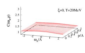
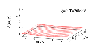
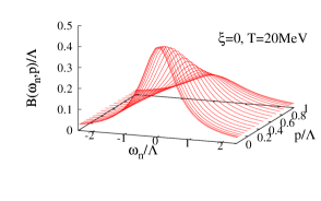
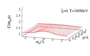
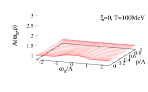
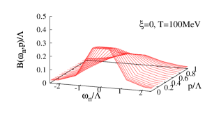
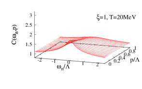
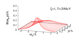
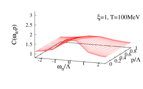
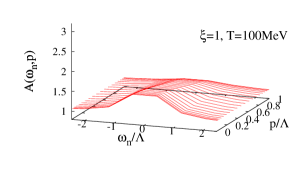
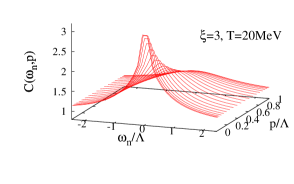
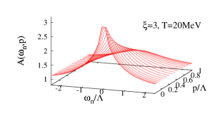
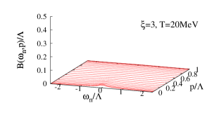
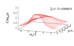
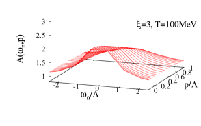
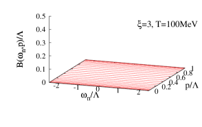
Figure 1: Numerical solutions of $C,A,B$ for $\alpha=2$, $\xi=0$, $1$, $3$ at $T=20$ and $100$MeV.

One notes that the values for $C$ and $A$ are almost $1$ for the Landau gauge, and it becomes large when $\xi$ has finite values, $\xi=1$ and $3$. On the other hand, $B$ has the opposite tendency; it is large for $\xi=0$ and it decreases with increasing $\xi$. This numerically comes from the fact that the denominator of the propagator enhances when $C$ and $A$ are large, then $B$ is small for that case consequently. As for the temperature dependence, $B$ decreases with respect to $T$, while $C$ and $A$ do not show drastic difference between low and high temperature. The results for $B$ is easily understood, since the restoration of the chiral symmetry breaking would be expected. On the other hand, the numerical solutions for $C$ and $A$ show that they do not decrease significantly up to intermediate temperature. We will discuss in more detail on the temperature dependence on $C$, $A$ and $B$ in the next subsection.

III.2 Temperature dependence on the solutions

Let us display the two dimensional figures so that one can see the temperature dependence in more clearly. Figure 2 shows the results for $C(\omega_{0},\delta)$, $A(\omega_{0},\delta)$, $B(\omega_{0},\delta)$ and the dynamical mass $M(\omega_{n},p)\equiv B(\omega_{n},p)/A(\omega_{n},p)$ as the function of the temperature.

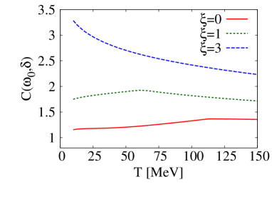
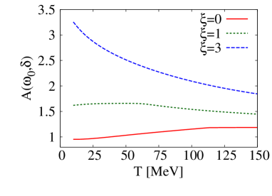
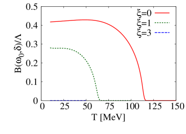
Figure 2: $C$, $A$, $B$ and $M$ with $\alpha=2$ for $\xi=0$, $1$ and $3$.

We see the rapid decrease on the results for $B$ and $M$ with increasing temperature as already mentioned in the previous subsection, while $C$ and $A$ exhibit rather mild change; they monotonically decreases according to $T$ for $\xi=3$, and stay almost the same values for $\xi=0$ and $1$. The difference between $B$ and $C$, $A$ comes from the different form of the equations; $B$ has the form of $B=\int\mathrm{d}^{4}qf_{B}(q)B(q)$ for massless case, while $C$ and $A$ have the complex form as $C=1+\int\mathrm{d}^{4}q[f_{C}(q)C(q)+f_{A}(q)A(q)]$. Therefore, consequently, $C$ and $A$ become close to $1$ for the case with small values of $\xi$, which is numerically confirmed in the above figure.

III.3 Critical behavior

Finally, we are going to study the critical temperature of the chiral phase transition through seeing the results of the dynamical mass. For our purpose, observing the value of $M(\equiv B/A)$ is enough since the chiral condensate is defined by,

$$\phi=\langle\bar{\psi}\psi\rangle=-T\sum_{m=-\infty}^{\infty}\int\frac{\mathrm{d}^{3}q}{(2\pi)^{3}}{\rm tr}\left[\frac{B(\omega_{m},q)}{C^{2}(\omega_{m},q)\omega_{m}^{2}+A^{2}(\omega_{m},q)q^{2}+B^{2}(\omega_{m},q)}\right],$$ (19)

then it becomes zero when $M=0$ while it has non-zero value for $M\neq 0$.

Figure 3 shows the numerical results of the dynamical mass for various couplings and gauges.

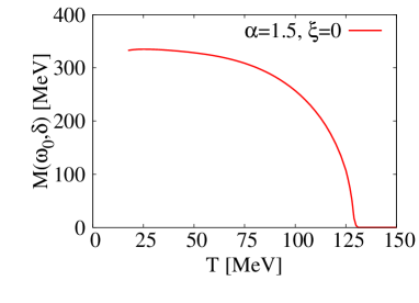
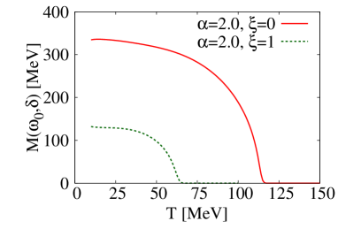
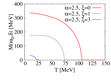
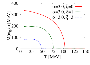
Figure 3: $M$ for various $\alpha(=1.5,\,2,\,2.5,\,3)$ and $\xi(=0,\,1,\,3)$.

It should be noted that the value $M=335$MeV at low $T$ for $\xi=0$ is due to our choice of parameter, and the remaining results are the predictions. One sees that the critical temperature, $T_{c}$, does not alter drastically with changing $\alpha$ for $\xi=0$; $T_{c}$ is in the range of $110-130$MeV for the Landau gauge. On the other hand, $T_{c}$ are considerably different for other gauges. The dynamical mass itself is not generated for smaller coupling; $M=0$ always holds for $\alpha=1.5$ with $\xi=1$ and $3$, and for $\alpha=2$ with $\xi=3$. From the figure we confirm the tendency that the critical temperature becomes small when $\xi$ is large.

To make the clearer comparison, we align the critical temperature in Tab. 2.

Table 2: Critical temperature [MeV].

	$\xi=0$	$\xi=1$	$\xi=2$	$\xi=3$
$\alpha=1.5$	$131$	—	—	—
$\alpha=2.0$	$117$	$66$	—	—
$\alpha=2.5$	$107$	$75$	$51$	$24$
$\alpha=3.0$	$105$	$78$	$62$	$50$

We notice that the decrease of the critical temperature with respect to $\xi$ becomes rather mild for larger $\alpha$, there the broken phase remains for all the case as shown in the table. It may be worth mentioning that the results for the Landau gauge exhibit similar values obtained by the analyses in Blank:2010bz . The obtained values are smaller than the expected number of $T_{c}\simeq 175$MeV from other theoretical predictions, such as the lattice QCD simulations. This is mainly due to the setting of the massless equations, and the parameter choice based on the dynamical mass $M=335$MeV at $T=0$ in the Landau gauge.

IV Concluding remarks

We performed the systematical numerical analyses on the quenched SDE of QCD without applying any approximation in general gauge, then studied the gauge dependence on the critical temperature of the chiral phase transition in this paper. We found that the critical temperature crucially depends on the gauge, and the parameters of the equations. Our numerical results show smaller values on the critical temperature, which is around $T_{c}\simeq 120$MeV or less, than the expected value $T_{c}\simeq 175$MeV. Then we think that careful considerations on both the gauge and parameter dependence are important when one studies the chiral phase transition by using the SDE.

The physical predictions from the SDE should be gauge, regularization and parameter independent in principle as mentioned in the introduction. However, the practical equations with several approximations lead gauge and parameter dependence as confirmed in this letter. For studying the practical usage of the SDE, we employed the quenched form without applying any further approximations, since it is the simplest and frequently used equations. Concerning on the above gauge dependence of the SDE, a lot of efforts have been made to obtain the gauge independent solutions (see, e.g., Rebhan:1992ak ; Kizilersu:2014ela ; Hoshino:2014nga ). We think this will be the future direction on the current approach beyond the quenched level.

- (1) F. J. Dyson, Phys. Rev. 75, 1736 (1949). J. S. Schwinger, Proc. Nat. Acad. Sci. 37, 452 (1951).
- (2) C. D. Roberts and A. G. Williams, Prog. Part. Nucl. Phys. 33, 477 (1994).
- (3) C. D. Roberts and S. M. Schmidt, Prog. Part. Nucl. Phys. 45, S1 (2000).
- (4) P. Maris and C. D. Roberts, Int. J. Mod. Phys. E 12, 297 (2003).
- (5) C. S. Fischer, J. Phys. G 32, R253 (2006).
- (6) K. Johnson, M. Baker and R. Willey, Phys. Rev. 136, B1111 (1964).
- (7) T. Maskawa and H. Nakajima, Prog. Theor. Phys. 52, 1326 (1974); ibid. 54, 860 (1975).
- (8) R. Fukuda and T. Kugo, Nucl. Phys. B 117, 250 (1976).
- (9) J. S. Ball and T. W. Chiu, Phys. Rev. D 22, 2542 (1980).
- (10) C. D. Roberts and B. H. J. McKellar, Phys. Rev. D 41, 672 (1990).
- (11) D. C. Curtis and M. R. Pennington, Phys. Rev. D 42, 4165 (1990).
- (12) C. J. Burden and C. D. Roberts, Phys. Rev. D 47, 5581 (1993).
- (13) M. Bando, M. Harada and T. Kugo, Prog. Theor. Phys. 91, 927 (1994).
- (14) K. Fukazawa, T. Inagaki, S. Mukaigawa and T. Muta, Prog. Theor. Phys. 105, 979 (2001).
- (15) A. Kizilersü and M. R. Pennington, Phys. Rev. D 79, 125020 (2009).
- (16) A. Bashir, R. Bermudez, L. Chang and C. D. Roberts, Phys. Rev. C 85, 045205 (2012).
- (17) A. Kizilersü, T. Sizer, M. R. Pennington, A. G. Williams and R. Williams, Phys. Rev. D 91, no. 6, 065015 (2015); and references therein.
- (18) T. Akiba, Phys. Rev. D 36, 1905 (1987).
- (19) O. K. Kalashnikov, Z. Phys. C 39, 427 (1988).
- (20) A. Barducci, R. Casalbuoni, S. De Curtis, R. Gatto and G. Pettini, Phys. Rev. D 41, 1610 (1990).
- (21) D. Blaschke, C. D. Roberts and S. M. Schmidt, Phys. Lett. B 425, 232 (1998).
- (22) P. Maris, C. D. Roberts and P. C. Tandy, Phys. Lett. B 420, 267 (1998).
- (23) M. Harada and A. Shibata, Phys. Rev. D 59, 014010 (1999).
- (24) T. Ikeda, Prog. Theor. Phys. 107, 403 (2002).
- (25) M. Harada and S. Takagi, Prog. Theor. Phys. 107, 561 (2002).
- (26) S. Takagi, Prog. Theor. Phys. 109, 233 (2003).
- (27) Y. Fueki, H. Nakkagawa, H. Yokota and K. Yoshida, Prog. Theor. Phys. 110, 777 (2003).
- (28) A. Krassnigg and C. D. Roberts, Nucl. Phys. A 737, 7 (2004).
- (29) A. Krassnigg, C. D. Roberts and S. V. Wright, Int. J. Mod. Phys. A 22, 424 (2007).
- (30) M. Harada, Y. Nemoto and S. Yoshimoto, Prog. Theor. Phys. 119, 117 (2008).
- (31) M. Blank and A. Krassnigg, Phys. Rev. D 82, 034006 (2010).
- (32) J. A. Mueller, C. S. Fischer and D. Nickel, Eur. Phys. J. C 70, 1037 (2010).
- (33) V. Mader, G. Eichmann, M. Blank and A. Krassnigg, Phys. Rev. D 84, 034012 (2011).
- (34) H. Nakkagawa, H. Yokota and K. Yoshida, Phys. Rev. D 85, 031902 (2012); ibid. 86, 096007 (2012).
- (35) M. L. Bellac, Thermal Field Theory, Cambridge University Press (1996).
- (36) J. M. Cornwall, R. Jackiw and E. Tomboulis, Phys. Rev. D 10, 2428 (1974).
- (37) A. Rebhan, Phys. Rev. D 46, 4779 (1992).
- (38) Y. Hoshino, T. Inagaki and Y. Mizutani, PTEP 2015, no. 2, 023B03 (2015).