YITP-16-2
Emergent classical geometries on boundaries
of randomly connected tensor networks

It is shown that classical spaces with geometries emerge on boundaries of randomly connected tensor networks with appropriately chosen tensors in the thermodynamic limit. With variation of the tensors, the dimensions of the spaces can be freely chosen, and the geometries, which are curved in general, can be varied. We give the explicit solvable examples of emergent flat tori in arbitrary dimensions, and the correspondence from the tensors to the geometries for general curved cases. The perturbative dynamics in the emergent space is shown to be described by an effective action which is invariant under the spatial diffeomorphism due to the underlying orthogonal group symmetry of the randomly connected tensor network. It is also shown that there are various phase transitions among spaces, including extended and point-like ones, under continuous change of the tensors.

1 Introduction

The construction of quantum gravity is one of the most fundamental problems in theoretical physics. Efforts made for this problem so far suggest that the classical notion of spacetime described by general relativity should somehow be replaced with a new one suitable for quantization. The classical notion, namely the continuous entity of spacetime with geometries, should appear as an infrared effective description of the new picture. The main subject of this paper is to explicitly show that the classical notion of spaces with geometries appears as an emergent phenomenon from the dynamics of the randomly connected tensor network. Here, the randomly connected tensor network is defined as random summation of tensor networks: tensors are treated as controllable external variables, while connections of tensors are randomly summed over. We will show that spaces with geometries appear on boundaries of randomly connected tensor networks, if tensors are appropriately chosen. By varying the tensors, one can freely choose the dimensions of the spaces, and can also vary the geometries. We will explicitly give the correspondence from the tensors to the geometries for general curved cases.

The background motivation for this work comes from the fact that the randomly connected tensor network is tightly related to a tensor model in the Hamilton formalism. Tensor models [1, 2, 3] have originally been introduced to describe $D>2$ simplicial quantum gravity as extensions of the matrix models which successfully describe the $D=2$ simplicial quantum gravity. Though the original tensor models suffer from some difficulties, the coloured tensor models [6], which appeared later with improvements, have extensively been analyzed [7]. However, the analyses so far have shown that the dominant configurations do not generate realistic structures comparable to our actual spacetime: branched polymers, for example, dominate [7, 8, 9] in the simplest settings. On the other hand, the numerical analyses of $D>2$ simplicial quantum gravity have shown that the Lorentzian models called causal dynamical triangulations (CDT) successfully generate de-Sitter like spacetimes like our actual universe [10], while the Euclidean ones do not. This success of CDT motivated one of the present authors to formulate a tensor model in the Hamilton formalism [13, 14], which we call canonical tensor model (CTM). CTM has been shown to have various interesting properties. It is unique under reasonable assumptions [14], and has tight connections with general relativity [15, 16]. In addition, it has connections to the randomly connected tensor network [17, 18]: the Hamiltonian of CTM generates a sort of a renormalization group flow of the randomly connected tensor network [19, 20]. The randomly connected tensor network is also useful in constructing the exact physical states of the quantized version of CTM [21, 22].

So far, a number of network-based models for emergent space or spacetime have been proposed, e.g. spin networks [23], loop quantum gravity (see e.g. [24]), causal sets [25, 26], energetic causal sets [27, 28], quantum graphity [29, 30, 31], information-bits model by Trugenberger [32, 33], Wolfram’s evolving networks [34], D’Ariano-Tosini causal networks [35], structurally dynamic cellular networks (see e.g. [36]), lumpy networks (see e.g. [37]), complex quantum network manifold [38, 39] and network geometry with flavor [40]. All the above constructions capture aspects of geometry from the bulk of networks. In contrast, in our model not the bulk but boundaries of networks provide the information of geometry.

This paper is organized as follows. In Section 2, we define the randomly connected tensor network, and explain our method to analyze it, which has been developed in [18, 19, 20]. In Section 3, we explain some difficulties in regarding the randomly connected tensor network itself as a space, and argue that its boundary is more qualified. In Section 4, we explicitly give such tensors that generate flat spaces of arbitrary dimensions on the boundaries of the randomly connected tensor networks. In Section 5, we consider variation of the tensors from those of the flat spaces to generate curved spaces. We explicitly give the correspondence from the tensors to the geometries of the spaces. In Section 6, we study phase transitions in which the flat spaces break down to point-like spaces and others. The final section is devoted to the summary and discussions. In Appendix A, we describe a covariant structure under the spatial diffeomorphism in the continuum description of the randomly connected tensor network, which is used in Section 5.

2 Randomly connected tensor network

We consider a real symmetric rank-three tensor, $P_{abc}$, where $a,b,c=1,2,\cdots,N$. As a tensor product of $P_{abc}$’s we introduce the following rank-$3n$ tensor:

$$W_{a_{1}a_{2}\cdots a_{3n}}(P)=P_{a_{1}a_{2}a_{3}}P_{a_{4}a_{5}a_{6}}\cdots P_{a_{3n-2}a_{3n-1}a_{3n}},$$ (1)

where $n$ is even integer. Contracting all indices in (1) in pairs by $\frac{3}{2}n$ delta functions $\delta_{a_{i}a_{j}}$, we construct O($N$)-invariant quantities. We denote such O($N$)-invariant quantities by $W_{g}(P)$ where $g$ specifies one way of contracting all indices in pairs. In fact, one can consider $g$ as a regular network consisting of $n$ three-vertices. Namely, we introduce $n$ trivalent vertices and assign $P_{abc}$ to each vertex in such a way that three lines emerging from a single trivalent vertex carry the indices, $a$, $b$ and $c$, respectively, and connect them by lines if the indices are contracted. In this way, one can construct a regular network $g$ allowing self-contractions. The self-contraction means that two of the three lines originating from a single vertex are connected by a line. See Fig.1 for an example of the networks.

Figure 1: An example of a tensor network with $n=6$.

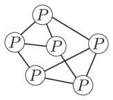
By this understanding, we define the partition function as a sum over all networks $g$:

$$Z_{n}(P)=\sum_{g}\frac{1}{|\text{Aut}(g)|}W_{g}(P),$$ (2)

where $|\text{Aut}(g)|$ is the order of the automorphism group of $g$. We call the model defined by the partition function (2) randomly connected tensor networks, and the randomness comes from the sum over all networks with the tensor assigned to each vertex. In fact one can choose $P_{abc}$ so that the partition function (2) describes a statistical system on random networks [17, 18, 19], such as the Ising model on random networks.

For convenience, we rewrite the partition function (2) in terms of the real integral [19, 18, 20]:

$$Z_{n}(P)=\frac{1}{n!}\int_{-\infty}^{\infty}\frac{\text{d}^{N}\varphi}{(2\pi)^{N/2}}\left(\frac{1}{3!}P\varphi^{3}\right)^{n}e^{-\frac{1}{2}\varphi^{2}},$$ (3)

where $\varphi_{a}\ (a=1,2,\ldots,N)$ are real integration variables, and we have used the shorthand notations given by

$$P\varphi^{3}:=P_{abc}\varphi_{a}\varphi_{b}\varphi_{c},\ \ \ \varphi^{2}:=\varphi_{a}\varphi_{a},\ \ \ \text{d}^{N}\varphi:=\prod^{N}_{a=1}\text{d}\varphi_{a}.$$ (4)

Here, repeated indices above are assumed to be summed over, and hereafter we will use this convention for the sum. Applying Wick’s theorem, one can confirm that the partition functions, (2) and (3), coincide. The partition function (3) is invariant under the O($N$) transformation of $P$,

$$P^{\prime}_{abc}=L_{a}{}^{a^{\prime}}L_{b}{}^{b^{\prime}}L_{c}{}^{c^{\prime}}P_{a^{\prime}b^{\prime}c^{\prime}},\ \ L\in\text{O}(N).$$ (5)

Let us consider the thermodynamic limit of the randomly connected tensor network, in which the size of the networks grows to infinity, $n\rightarrow\infty$. It can be shown that the partition function (3) in this limit can be exactly computed by a mean field method [19, 18, 17]. To see this, we implement the rescaling, $\varphi_{a}\to\varphi^{\prime}_{a}=\sqrt{2n}\ \phi_{a},$ and correspondingly the partition function (3) becomes

$$Z_{n}(P)=C_{n}\int^{\infty}_{-\infty}\text{d}^{N}\phi\ e^{-nf(P,\phi)},$$ (6)

where

$$C_{n}=\frac{(2n)^{\frac{3n}{2}}}{n!\left(3!\right)^{n}}\left(\frac{n}{\pi}\right)^{\frac{N}{2}},$$ (7)

$$f(P,\phi)=\phi^{2}-\frac{1}{2}\log\left[A(\phi)^{2}\right],\ \ \ \text{with}\ \ \ A(\phi)=P\phi^{3}.$$ (8)

From the expression (6), in the thermodynamic limit $n\rightarrow\infty$, the steepest descent method can be applied, and the partition function is determined by the neighborhood of the minimum of $f(P,\phi)$ as a function of $\phi$. Thus the free energy per vertex in the thermodynamic limit can be defined as

$$f(P):=-\lim_{n\rightarrow\infty}\frac{1}{n}\ln\left(\frac{Z_{n}(P)}{C_{n}}\right)=\min_{\phi}f(P,\phi)=f(P,\phi_{min}).$$ (9)

In the expression above we have removed the numerical factor $C_{n}$ from the definition of the free energy, since this simply gives a $P$-independent shift of the free energy. The minimum $\phi=\phi_{min}$ is one of the solutions $\phi=\bar{\phi}$ to the stationary condition,

$$\left.\frac{\partial f(P,\phi)}{\partial\phi_{a}}\right|_{\phi=\bar{\phi}}=2\bar{\phi}_{a}-\frac{3(P\bar{\phi}^{2})_{a}}{A(\bar{\phi})}=0,$$ (10)

where we have used the following shorthand notation:

$$(P\phi^{2})_{a}:=P_{abc}\phi_{b}\phi_{c}.$$ (11)

Multiplying (10) by $\bar{\phi}$, one obtains

$$\bar{\phi}^{2}=\frac{3}{2}.$$ (12)

In simplifying expressions, (10) is useful in the form,

$$(P\bar{\phi}^{2})_{a}=\frac{2}{3}A(\bar{\phi})\bar{\phi}_{a}.$$ (13)

Note that $\bar{\phi}$ and $\phi_{min}$ are generally dependent on $P$, but we suppress the argument for notational simplicity.

In general, in the vicinities of first order phase transition surfaces, not only the absolute minimum of the free energy but also stable local minima are physically relevant. The local stability of each stationary point can be checked by evaluating the positivity of the Hessian, i.e. the matrix of the second order derivatives of $f(P,\phi)$ with respect to $\phi$ evaluated at $\phi=\bar{\phi}$. Using (13) to simplify the expression, the Hessian is obtained as

$$f^{(2)}_{ab}:=\left.\frac{\partial^{2}f(P,\phi)}{\partial\phi_{a}\partial\phi_{b}}\right|_{\phi=\bar{\phi}}=2\left(\delta_{ab}+2\bar{\phi}_{a}\bar{\phi}_{b}-\frac{3(P\bar{\phi})_{ab}}{A(\bar{\phi})}\right).$$ (14)

One of its eigenvectors is $\bar{\phi}$ with eigenvalue $4$:

$$f^{(2)}_{ab}\bar{\phi}_{b}=2\left(\bar{\phi}_{a}+2\bar{\phi}^{2}\bar{\phi}_{a}-\frac{3(P\bar{\phi}^{2})_{a}}{A(\bar{\phi})}\right)=4\bar{\phi}_{a},$$ (15)

where we have used (12), (13), and (14).

3 Boundaries of random networks as spaces

It is not an easy question how random networks can be regarded as spaces. The most naive manner of identification would be to regard vertices as points forming a space and connecting lines as representations of local structures of their neighbourhoods. In fact, this is the common perspective used in lattice theories. However, this lattice-like way of viewing random networks as spaces seems to have at least the following difficulties:

• Difference of structures between random networks and our space : Random networks do not seem to have similar structures as our actual space, which is smooth, respects locality, and has three dimensions. In fact, it is known that, in the thermodynamic limit, random networks with a fixed degree of vertices effectively approach the Bethe lattice, which is tree-like [17]. This is far from the actual structure of our space.

• Finite correlation lengths : The Ising model on random networks with a finite degree of vertices has a finite correlation length even on the second order phase transition point in the thermodynamic limit [17]. Since this seems to be an outcome of the tree-like structure of the Bethe lattice in the thermodynamic limit, finiteness of correlation lengths will generally hold in the other statistical systems on random networks. This means that it is not possible to get any modes which propagate infinitely far. Therefore, it is not plausible to obtain physically sensible theories for the actual space from such a framework.

• Difficulty in labeling positions in random networks: In our framework, each vertex is just a representation of a tensor $P$. Therefore, the vertices are basically all the same and cannot be distinguished from each other in a well-defined way in the random sum over networks. This difficulty in labelling the vertices would be an obstacle in obtaining any classical geometries.

In view of these difficulties, the naive picture to identify randomly connected tensor networks as spaces may not be a right way. Especially, the last difficulty above suggests that we should more seriously consider what are the appropriate quantities to observe in randomly connected tensor networks. The natural physically relevant quantities of the system defined by the partition function (3) are the correlation functions of $\varphi$:

$$\left\langle\varphi_{a_{1}}\varphi_{a_{2}}\cdots\varphi_{a_{k}}\right\rangle=\frac{1}{Z_{n}}\int_{-\infty}^{\infty}\frac{\text{d}^{N}\varphi}{(2\pi)^{N/2}}\,\varphi_{a_{1}}\varphi_{a_{2}}\cdots\varphi_{a_{k}}\,\frac{1}{n!}\left(\frac{1}{3!}P\varphi^{3}\right)^{n}e^{-\frac{1}{2}\varphi^{2}}.$$ (16)

Applying Wick’s theorem as before, the correlation function above corresponds to the summation over tensor networks with external lines having fixed indices (See Fig.2). In other words, this is the random summation over tensor networks with fixed configurations on their boundaries. So, we are pursuing the possibility of regarding boundaries of random networks as spaces rather than networks themselves, or, in other words, the possibility that “points” labelled by the index set on the boundaries form a space. Note that, due to the random summation over networks, the local structure of neighborhoods on such boundaries may be significantly different from that of networks themselves. This difference may solve the geometrical difficulties mentioned in the first and second items of the list above. In the rest of this paper, we will show that, by appropriate choices of the tensor $P$, the correlation functions behave as if $\varphi$ is a field in spaces with regular properties, i.e. the spaces are smooth, respect locality and have certain dimensions.

Figure 2: The graphical representation of the correlation function $\langle\varphi_{a_{1}}\varphi_{a_{2}}\cdots\varphi_{a_{k}}\rangle$.

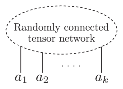
To compute the correlation function (16) in the thermodynamic limit, we investigate the partition function. To begin, we implement the rescaling, $\varphi\to\varphi^{\prime}=\sqrt{2n}\phi$, as before, and perturb $\phi$ around one of local minima $\bar{\phi}$ defined by (10) as

$$\phi_{a}=\bar{\phi}_{a}+\frac{v_{a}}{\sqrt{n}}.$$ (17)

Inserting (17), the partition function (6) for the large-$n$ can be expressed as

$$C_{n}n^{-\frac{N}{2}}e^{-nf(P,\bar{\phi})}\int_{-\infty}^{\infty}\text{d}^{N}v\,e^{-\frac{1}{2}f^{(2)}_{ab}v_{a}v_{b}+\mathcal{O}\left(\frac{v^{3}}{\sqrt{n}}\right)+\cdots}.$$ (18)

From (18) one can see that, in the thermodynamic limit, the system is described by a free theory of $v$. For instance, the connected part of the two point correlation function of $\varphi$ is given by

$$\begin{split}\left\langle\varphi_{a}\varphi_{b}\right\rangle_{\text{con.}}&=\left\langle\varphi_{a}\varphi_{b}\right\rangle-\left\langle\varphi_{a}\right\rangle\left\langle\varphi_{b}\right\rangle\\ &=2\left\langle v_{a}v_{b}\right\rangle_{\text{con.}}\\ &=2f^{(2)\,-1}_{ab}+\mathcal{O}\left(n^{-1}\right),\end{split}$$ (19)

where $f^{(2)\,-1}$ is the inverse matrix of $f^{(2)}$. Here we have also used that, from (18), the one point function is sub-dominant, $\langle v_{a}\rangle\sim\mathcal{O}\left(n^{-1/2}\right).$ Higher order correlation functions behave similarly as a free theory in the leading order.

Thus, the challenge is whether we can find appropriate $P$’s so that the correlation function (19) behaves in the same manner as that in a regular space. This task contains the dynamical complexity that the minimum solution $\bar{\phi}$ depends non-trivially on $P$. In Section 4, we will give exactly solvable cases representing flat $D$-dimensional tori, and, in Section 5, we will treat spaces with general metrics. The dynamical complexity concerning the stability of the spaces will be discussed in Section 6.

4 Flat spaces

In this section, we explicitly give $P$’s which realize arbitrary dimensional flat spaces. The criterion for the emergence is whether the correlation function (19) is similar to that in a flat space. This is equivalent to showing that the eigenvalues and eigenvectors of $f^{(2)}$ are similar to those in a flat space. We will first discuss the one-dimensional case, circles, and then consider $D$-dimensional flat tori.

4.1 Circles

We parametrize $P_{abc}$ as

$$P_{abc}=P^{L}_{abc}+\xi\left(P^{L}_{add}\delta_{bc}+P^{L}_{bdd}\delta_{ca}+P^{L}_{cdd}\delta_{ab}\right),$$ (20)

where $\xi$ is a real parameter, and $P^{L}_{abc}$ is a local part of the tensor. The components of the local part are given by

$$P^{L}_{i,i,i}=1,\quad P^{L}_{i,i+1,i+1}=P^{L}_{i,i,i+1}=\kappa,\ \ \ i=1,2,\ldots,N.$$ (21)

Here we use Latin $i,j,k$ on indices for components of a tensor, and the repetition of them does not imply summing over. These indices are identified in modulo $N$, namely $N\sim 0$, to consider a circle composed of $N$ “points”. $\kappa$ is a real parameter. Then,

$$\begin{split}P_{iii}&=1+3\gamma_{N},\\ P_{ijj}&=\begin{cases}\kappa+\gamma_{N}&i\sim j\\ \gamma_{N}&\text{otherwise}\end{cases},\\ P_{ijk}&=0,\end{split}$$ (22)

where $i,j,k$ are always supposed to be different from each other, and $\gamma_{N}=\xi\sum_{j}P^{L}_{ijj}=\xi(1+2\kappa)$. The symbol $i\sim j$ denotes a relationship of $i$ being $j$’s neighbour, which, in this case, means $i=j\pm 1$ (modulo $N$). As can be seen in (22), the term proportional to $\xi$ in (20) generates a non-local part of $P$.

Because of the discrete translational symmetry in $P$, a solution to the stationary condition (10) is given by

$$\bar{\phi}^{\pm}_{a}=\pm\sqrt{\frac{3}{2N}}.$$ (23)

This solution is stable as a local minimum, when the spectra being obtained below are all positive. On the other hand, whether this is an absolute minimum or not is a complex problem, and will be studied in Section 6.

For the solution (23), it is not hard to calculate that

$$A(\bar{\phi}^{\pm})=\pm N^{-1/2}\left(\frac{3}{2}\right)^{3/2}(1+6\kappa+3\gamma),$$ (24)

where $\gamma=N\gamma_{N}$.

For the convenience of our future discussion, we introduce two symbols. $\tilde{\delta}_{ab}$ equals $1$ when $a\sim b$, and vanishes otherwise. $1_{ab}$ constantly equals to unit. Using these symbols, we get

$$P_{abc}\bar{\phi}_{c}^{\pm}=\pm N^{-1/2}\left(\frac{3}{2}\right)^{1/2}\left[(1+2\kappa+\gamma)\delta_{ab}+2\kappa\tilde{\delta}_{ab}+\frac{2\gamma}{N}1_{ab}\right].$$ (25)

Let us introduce

$$p=\frac{1+2\kappa+\gamma}{1+6\kappa+3\gamma}\,,\quad q=\frac{4\kappa}{1+6\kappa+3\gamma}\,,\quad r=\frac{2\gamma}{1+6\kappa+3\gamma}.$$ (26)

They satisfy $p+q+r=1$. Then the Hessian (14) can be computed as

$$f^{(2)}_{ab}=(2-4p)\delta_{ab}-2q\tilde{\delta}_{ab}+\frac{6-4r}{N}1_{ab}.$$ (27)

Now, let us consider discrete analogues of plane waves, $\psi^{(l)}_{a}=e^{i\frac{2\pi l}{N}a}$. We find that they are the eigenvectors of $f^{(2)}$:

$$f^{(2)}_{ab}\psi^{(l)}_{b}=\left(2-4p-4q\cos\frac{2\pi l}{N}\right)\psi^{(l)}_{a}\,,\quad\text{for $l=1,2,\dots,N-1$},$$ (28)

and $f^{(2)}_{ab}\psi^{(0)}_{b}=f^{(2)}_{ab}1_{b}=4\cdot 1_{a}$. Thus, naming

$$\Lambda=\left\{\left.\lambda_{l}=2-4p-4q\cos\frac{2\pi l}{N}\,\right|\,l=1,2,\dots,N-1\right\},$$ (29)

the spectra of $f^{(2)}_{ab}$ are represented by the set $\Lambda\cup\{4\}$. An example of the spectra is plotted in Figure 3.

Figure 3: An example of the spectra (29) for $N=20,\,p=0,\,q=\frac{1}{4}$.

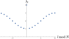
As can be seen in the example, the spectra of $f^{(2)}$ are similar to those of $\nabla^{2}+m^{2}$ in one dimension, except that the zero mode is supermassive and that higher spectra are deformed. Thus, the minimal of these spectra should be regarded as the rest mass, and an analogue of $\nabla^{2}$ on the emergent space can be evaluated by subtracting the mass from these spectra. Then, one way to understand the geometric property in general is to compute the spectral dimension defined by

$$D(\sigma)\equiv-2\frac{\sigma}{\Sigma}\frac{\partial\Sigma}{\partial\sigma},$$ (30)

where

$$\Sigma=e^{-(4-\lambda_{\text{min}})\sigma}+\sum_{\lambda\in\Lambda}e^{-(\lambda-\lambda_{\text{min}})\sigma},$$ (31)

and $\lambda_{\text{min}}=\min(\inf(\Lambda),4)$. For different $p$ and $q$, we can show numerical computations as examples, e.g. Fig 4. In the fine case of the figure, we certainly obtain $D(\sigma)\sim 1$ in the large-scale region $\sigma\gg 1$.

Figure 4: The behavior of $D(\sigma)$ is sensitive to the value of $\inf(\Lambda)$. The left one has its $2-4p-4|q|$ being positive and less than $4$, then everything is fine. The right one has its $2-4p-4|q|$ greater than $4$, and it is ill behaved.

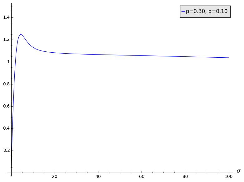
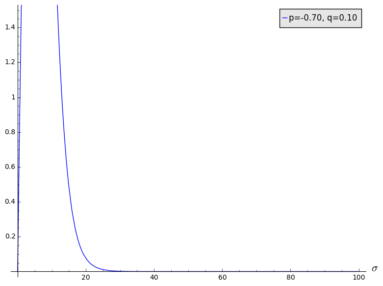
From the figure we realize that $4$ should not be the minimal, otherwise dimensions blow up as $N$ gets bigger. Noticing that the minimal of the set $\Lambda$ is given by $2-4p-4|q|$ when $N$ goes to infinity, one can immediately rewrite

$$\lim_{N\rightarrow\infty}\frac{2\pi}{N}\Sigma= \lim_{N\rightarrow\infty}\sum_{n=1}^{N-1}\frac{2\pi}{N}\cdot\exp\left(-4|q|\sigma+4q\sigma\cos\frac{2\pi n}{N}\right)$$

$$= e^{-4|q|\sigma}\int_{0}^{2\pi}\text{d}\theta~{}e^{4q\sigma\cos\theta}=2\pi e^{-4|q|\sigma}I_{0}(4|q|\sigma),$$ (32)

where $I_{0}$ is the modified Bessel function of the first kind. Therefore the spectral dimension $D(\sigma)$ has an asymptotic behavior as

$$\mathcal{D}_{1}(\sigma)\equiv\lim_{N\rightarrow\infty}D(\sigma)= -\frac{2\sigma}{e^{-4|q|\sigma}I_{0}(4|q|\sigma)}\frac{\text{d}}{\text{d}\sigma}\left(e^{-4|q|\sigma}I_{0}(4|q|\sigma)\right)$$

$$= 2\tau\left(1-\frac{I_{1}(\tau)}{I_{0}(\tau)}\right),$$ (33)

where $\tau=4|q|\sigma$. One can check that ${\cal D}_{1}(\sigma)$ behaves in the same manner as the example in the left figure of Fig. 4.

The minimal of the spectrum should be no less than zero for the stability of the solution (23) under small perturbations. On the other hand, from the previous discussion, a proper result also requires the minimum be in the set $\Lambda$ instead of being $4$. Together they give the restriction of

$$0\leqslant\inf(\Lambda)\leqslant 4.$$ (34)

When $N$ goes to infinity, this becomes

$$0\leqslant 2-4p-4|q|\leqslant 4$$

$$\Rightarrow 1\geqslant 2p+2|q|\geqslant-1,$$ (35)

which obviously depends on the sign of $1+6\kappa+3\gamma$. Define $s=\text{sgn}(1+6\kappa+3\gamma)$. It is clear that $|1+6\kappa+3\gamma|=s(1+6\kappa+3\gamma)>0$ thus $s^{2}\equiv 1$. Then Eq.(35) can be rewritten as

$$s\gamma \geqslant sf_{s}(\kappa)\equiv s(1-2\kappa)+8|\kappa|,$$ (36)

$$s\gamma \geqslant sg_{s}(\kappa)\equiv-s\left(\frac{3}{5}+2\kappa\right)-\frac{8}{5}|\kappa|,$$ (37)

$$s\gamma > sh_{s}(\kappa)\equiv-s\left(\frac{1}{3}+2\kappa\right).$$ (38)

We understand the following:

1. $s=+$:

   We have $f_{+}>h_{+}>g_{+}$ for any $\kappa$, thus the restriction is given by $\gamma\geqslant f_{+}$.

2. $s=-$:

   In area $|\kappa|>1/6,~{}f_{-}<h_{-}<g_{-}$; thus the restriction is $\gamma\leqslant f_{-}$. In area $|\kappa|<1/6,~{}f_{-}>h_{-}>g_{-}$; thus the restriction is $\gamma\leqslant g_{-}$. When $|\kappa|=1/6,~{}f_{-}=g_{-}=h_{-}$, however we know $\gamma$ should never equal to $h_{-}$. Therefore, the restriction is given by $\gamma<0$ and $\gamma<-2/3$ for $\kappa=-1/6$ and $\kappa=1/6$, respectively.

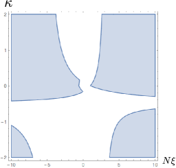
Taking the form of $\gamma=N\xi(1+2\kappa)$ into our final consideration, and noticing that the sign of $1+2\kappa$ also matters, we give Table 1 and Figure 5 describing the restriction in total.

$\kappa$		$(-\infty,-\frac{1}{2})$	$(-\frac{1}{2},-\frac{1}{6})$	$-\frac{1}{6}$	$(-\frac{1}{6},0)$	$(0,\frac{1}{6})$	$\frac{1}{6}$	$(\frac{1}{6},+\infty)$
$N\xi\geqslant C_{u,v}(\kappa)$	$u$	3	-5			3
	$v$	-2	6			-2
$N\xi\leqslant C_{u,v}(\kappa)$	$u$	-5	3	$0^{*}$	-9/5	-1/5	$-2/3^{*}$	-5
	$v$	6	-2		6/5	-2/5		6

Table 1: Here, $C_{u,v}(\kappa)=u+\frac{v}{1+2\kappa}$. The additional star mark means the equivalence to that restriction cannot be obtained.

Figure 5: The shaded regions represent the allowed region (35).

4.2 Flat $D$-Dimensional Tori

For simplicity, we still assume the localized $P^{L}$ is given by

$$P^{L}_{I,I,I}=1\,,\quad P^{L}_{I,I,I+e^{j}}=P^{L}_{I,I+e^{j},I+e^{j}}=\kappa_{D},$$ (39)

where $I=(i_{1},i_{2},\dots,i_{D})$ is a vector from a module defined on ring $\mathbb{Z}/\mathcal{N}\mathbb{Z}$, characterizing a point on the $D$-dimensional compact lattice. $\mathcal{N}^{D}=N$ describes how fine the structure is divided. $e^{j}$’s are the basis of this module. In this case, if $J=I\pm e^{j}$, we say $J$ is a neighbor of $I$. Again, we denote this relation by $J\sim I$.

Generate the total tensor $P_{abc}$ via eq.(20):

$$P_{I,I,I} = 1+3\gamma_{D},$$ (40)

$$P_{I,J,J} = \begin{cases}\kappa_{D}+\gamma_{D}&J\sim I\\ \gamma_{D}&\text{otherwise}\end{cases},$$ (41)

$$P_{I,J,K} = 0,$$ (42)

where $\gamma_{D}=\xi\sum_{J}P^{L}_{IJJ}=\xi(1+2D\kappa_{D})$.

Assuming that the field $\bar{\phi}$ in (23) with a uniform value on every point is the minimal of $f(P,\phi)$, we have

$$P_{abc}\bar{\phi}_{c}=N^{-1/2}\sqrt{\frac{3}{2}} \left[(1+3\gamma_{D}+2D(\kappa_{D}+\gamma_{D})+(N-2D-1)\gamma_{D})\delta_{ab}\right.\,$$

$$+2(\kappa_{D}+\gamma_{D})\tilde{\delta}_{ab}\left.+2\gamma_{D}(1_{ab}-\delta_{ab}-\tilde{\delta}_{ab})\right]$$

$$=N^{-1/2}\sqrt{\frac{3}{2}} \left[(1+2D\kappa_{D}+N\gamma_{D})\delta_{ab}+2\kappa_{D}\tilde{\delta}_{ab}+2\gamma_{D}1_{ab}\right],$$ (43)

and

$$A(\bar{\phi})=N^{-1/2}\left(\frac{3}{2}\right)^{3/2}\left(1+6D\kappa_{D}+3N\gamma_{D}\right).$$ (44)

Let us introduce $p,q,r$ in the same form as eq.(26) with $\kappa=D\kappa_{D}$ and $\gamma=N\gamma_{D}$. We get

$$f^{(2)}_{ab}=(2-4p)\delta_{ab}-\frac{2q}{D}\tilde{\delta}_{ab}+\frac{6-4r}{N}1_{ab}.$$ (45)

Now consider vectors, $\Psi^{\hat{n}}_{J}=e^{i\frac{2\pi\hat{n}}{\mathcal{N}}\cdot{J}}$, where both $\hat{n}$ and $J$ are $D$-component vectors. We can calculate that

$$\sum_{J}f^{(2)}_{IJ}\cdot\Psi^{\hat{n}}_{J}=(2-4p)e^{i\frac{2\pi\hat{n}}{\mathcal{N}}\cdot I}-\frac{2q}{D}\sum_{j=1}^{D}\left(e^{i\frac{2\pi\hat{n}}{\mathcal{N}}\cdot(I+e^{j})}+e^{i\frac{2\pi\hat{n}}{\mathcal{N}}\cdot(I-e^{j})}\right)+\frac{6-4r}{N}\sum_{J}e^{i\frac{2\pi\hat{n}}{\mathcal{N}}\cdot J},$$ (46)

where the second term on the right-hand side can be rewritten as

$$\frac{2q}{D}\sum_{j=1}^{D}\left(e^{i\frac{2\pi\hat{n}}{\mathcal{N}}\cdot(I+e^{j})}+e^{i\frac{2\pi\hat{n}}{\mathcal{N}}\cdot(I-e^{j})}\right)=\frac{4q}{D}e^{i\frac{2\pi\hat{n}}{\mathcal{N}}\cdot I}\sum_{j=1}^{D}\cos\frac{2\pi n_{j}}{\mathcal{N}}.$$ (47)

The third term is

$$\sum_{J}e^{i\frac{2\pi\hat{n}}{\mathcal{N}}\cdot J}= \sum_{J}\prod_{k=1}^{D}e^{i\frac{2\pi n_{k}}{\mathcal{N}}J_{k}}=\prod_{k=1}^{D}\sum_{j=1}^{\mathcal{N}}e^{i\frac{2\pi n_{k}}{\mathcal{N}}j}$$

$$= \begin{cases}N&\hat{n}=0\\ 0&\text{otherwise}\end{cases}.$$ (48)

Thus, when $\hat{n}\neq 0$, we get $N-1$ eigenvalues given by

$$f^{(2)}_{ab}\Psi^{\hat{n}}_{b}=\left(2-4p-\frac{4q}{D}\sum_{j=1}^{D}\cos\frac{2\pi n_{j}}{\mathcal{N}}\right)\Psi^{\hat{n}}_{a}.$$ (49)

And when $\hat{n}=0$, we have

$$f^{(2)}_{ab}\Psi^{\hat{n}}_{b}=f^{(2)}_{ab}~{}1_{b}=4\cdot 1_{a}.$$ (50)

Again, we have the spectra described as $(\Lambda_{D}\backslash\{2-4p-4q\})\cup\{4\}$, where

$$\Lambda_{D}=\left\{\left.2-4p-\frac{4q}{D}\sum_{j=1}^{D}\cos\frac{2\pi n_{j}}{\mathcal{N}}\,\right|\,n_{j}=0,1,\dots,\mathcal{N}-1\right\}.$$ (51)

Following the same process as in the one dimensional case, we have $0\leqslant\lambda_{\text{min}}=2-4p-4|q|\leqslant 4$. The spectral dimension is still defined as (30). Then we have

$$\lim_{\mathcal{N}\rightarrow\infty}\left(\frac{2\pi}{\mathcal{N}}\right)^{D}\Sigma= \lim_{\mathcal{N}\rightarrow\infty}\left(\frac{2\pi}{\mathcal{N}}\right)^{D}\sum_{\lambda\in\Lambda_{D}}e^{(\lambda-\lambda_{\text{min}})\sigma}$$

$$= \lim_{\mathcal{N}\rightarrow\infty}e^{-4|q|\sigma}\prod_{j=1}^{D}\,\sum_{\{n_{j}\}}\,\frac{2\pi}{\mathcal{N}}\exp\left(\frac{4q}{D}\sigma\cos\frac{2\pi n_{j}}{\mathcal{N}}\right)$$

$$= e^{-4|q|\sigma}\prod_{j=1}^{D}\,\lim_{\mathcal{N}\rightarrow\infty}\sum_{n=0}^{\mathcal{N}-1}\,\frac{2\pi}{\mathcal{N}}\exp\left(\frac{4q}{D}\sigma\cos\frac{2\pi n}{\mathcal{N}}\right)$$

$$= e^{-4|q|\sigma}\left[2\pi I_{0}\left(\frac{4|q|}{D}\sigma\right)\right]^{D}.$$ (52)

Therefore, in $N\to\infty$, the spectral dimension behaves as

$$\mathcal{D}(\sigma)\equiv\lim_{N\rightarrow\infty}D(\sigma)=D\cdot\mathcal{D}_{1}(\sigma/D).$$ (53)

Since, $\lambda_{\text{min}}$ and $p,q,r$, all takes the same form as in the one dimensional case, the restriction condition for $\xi$ listed in Table 1 still applies with $\kappa=D\kappa_{D}$.

5 Spaces with general metrics

In Section 4, we have shown that the two-point correlation function, i.e. $f^{(2)-1}_{ab}$, indicates the emergence of Euclidean flat spaces on boundaries of networks. Putting the argument forward, we try to read off metrics for more general emergent spaces, when $N$ is large. To begin, we parametrize $P_{abc}$ in the same way as in (21) with more general $P^{L}_{abc}$, where $P^{L}_{abc}$ is an almost local part of the tensor such that $P^{L}_{abc}\neq 0$ only for $a\sim b\sim c$ (In this section, the symbol $\sim$ is used to represent nearby points as well as the same point, slightly more general than the usage in Section 4.). The strategy is that we will compute the quadratic term of $v$ in (18) to extract a metric in an effective field theory in a formal continuum limit.

To set aside a super-massive mode similar to the zero mode for the flat case in Section 4, we assume perturbations $v$ around the vacuum $\bar{\phi}$ to satisfy a constraint,

$$v_{a}\bar{\phi}_{a}=0.$$ (54)

This is a non-local kind of constraint, since, in the present general case too, we expect that $\bar{\phi}_{a}$ takes non-vanishing values for all the range of $a$. This non-local constraint would not ruin the significance of our model, since it would be impossible for a local observer to detect the existence of such a single non-local constraint, when $N$ is large. Then the contraction of $v_{a}$ with the Hessian (14) is given by

$$f^{(2)}_{ab}v_{a}v_{b}=\left(2-\frac{6\xi}{A(\bar{\phi})}P^{L}_{bdd}\bar{\phi}_{b}\right)v_{a}v_{a}-\frac{6}{A(\bar{\phi})}P^{L}_{abc}\bar{\phi}_{a}v_{b}v_{c}.$$ (55)

When $N\to\infty$, we implement the formal continuum limit:

$$P^{L}_{abc}\Rightarrow P^{L}(x,y,z),\ \ \ \bar{\phi}_{a}\Rightarrow\bar{\phi}(x),\ \ \ v_{a}\Rightarrow v(x),\ \ \ \sum_{a}\Rightarrow\int\text{d}^{D}x,$$ (56)

where the discrete labels $a,b,c$ have been replaced by the continuous coordinates $x,y,z\in\mathbb{R}^{D}$, respectively. Although $P^{L}(x,y,z)$ is a tri-local function, by definition, $P^{L}(x,y,z)=0$ unless $x\sim y\sim z$. In other words, $P^{L}(x,y,z)$ can be regarded as a distribution concentrated around $x\sim y\sim z$, and a moment expansion, which was introduced in another context in [16], will give a good approximation:

$$\int\text{d}^{D}y\text{d}^{D}z\ P^{L}(x,y,z)f_{1}(x)f_{2}(y)f_{3}(z)$$

$$\ \ \ \cong\alpha f_{1}f_{2}f_{3}+\beta^{\mu}f_{1}\partial_{\mu}\left(f_{2}f_{3}\right)+\frac{1}{2}\gamma^{\mu\nu}f_{1}\left(f_{2}\partial_{\mu}\partial_{\nu}f_{3}+f_{3}\partial_{\mu}\partial_{\nu}f_{2}\right)+\tilde{\gamma}^{\mu\nu}f_{1}\partial_{\mu}f_{2}\partial_{\nu}f_{3}+\cdots,$$ (57)

where $f_{1}$, $f_{2}$ and $f_{3}$ are test functions, $\alpha$, $\beta^{\mu}$, $\gamma^{\mu\nu}$ and $\tilde{\gamma}^{\mu\nu}$ are the moments, the argument $x$ is suppressed in the last line for brevity, and the dots represent higher moments being neglected in the present analysis. Due to the symmetry of $P^{L}(x,y,z)$ under the exchange of its arguments $x,y,z$, the moments are not independent and satisfy [16]

$$\beta^{\mu}=\frac{1}{2}\partial_{\nu}\gamma^{\mu\nu},\ \ \ \tilde{\gamma}^{\mu\nu}=\frac{1}{2}\gamma^{\mu\nu}.$$ (58)

As has been shown in [16], the O($N$) invariance (5) of the randomly connected tensor network implies that the formal continuum limit of the system be invariant under the spatial diffeomorphism. The spatial diffeomorphism is such that, after the formal replacement $a\Rightarrow x$, a vector, say $f_{a}$, becomes a scalar half-density $f(x)$. Therefore the test functions above should be treated as scalar half-densities, and the moments defined above are not covariant. In order to make the transformation property transparent, let us introduce a symmetric two-tensor $g_{\mu\nu}$, which will shortly be related to the moments, and rewrite the expansion (57) as

$$\int\text{d}^{D}y\text{d}^{D}z\ P^{L}(x,y,z)f_{1}(x)f_{2}(y)f_{3}(z)$$

$$\ \ \ \cong\alpha_{c}f_{1}f_{2}f_{3}+\beta^{\mu}_{c}f_{1}\nabla_{\mu}\left(f_{2}f_{3}\right)+\frac{1}{2}\gamma^{\mu\nu}_{c}f_{1}\left(f_{2}\nabla_{\mu}\nabla_{\nu}f_{3}+f_{3}\nabla_{\mu}\nabla_{\nu}f_{2}\right)+\tilde{\gamma}^{\mu\nu}_{c}f_{1}\nabla_{\mu}f_{2}\nabla_{\nu}f_{3}+\cdots,$$ (59)

where $\nabla_{\mu}$ is the covariant derivative associated with $g_{\mu\nu}$, and $\alpha_{c}$, $\beta^{\mu}_{c}$ and $\gamma^{\mu\nu}_{c}$ are the covariant moments. Below, we will shortly see that $g_{\mu\nu}$ actually plays the role of a metric in an effective action. Corresponding to (58), we also have

$$\beta^{\mu}_{c}=\frac{1}{2}\nabla_{\nu}\gamma^{\mu\nu}_{c},\ \ \ \tilde{\gamma}^{\mu\nu}_{c}=\frac{1}{2}\gamma^{\mu\nu}_{c}.$$ (60)

As shown in Appendix A, the covariant moments are just given by the linear combinations of the moments above up to the higher order corrections neglected in the present analysis, and therefore, the two descriptions, (57) and (59), are equivalent up to the order.

By using these covariant properties, it is possible to rewrite the continuum limit of $v$, $\bar{\phi}$ and the covariant moments, $\alpha_{c},\gamma^{\mu\nu}_{c}$, in the following covariant manner:

$$v=g^{1/4}\sigma_{1},\ \ \ \bar{\phi}=g^{1/4}\sigma_{2},\ \ \ \alpha_{c}=g^{-1/4}\sigma_{3},\ \ \ \gamma^{\mu\nu}_{c}=g^{-1/4}g^{\mu\nu}\sigma_{2},$$ (61)

where we have introduced scalars, $\sigma_{i}\ (i=1,2,3)$, and $g$ is the determinant of the metric $g_{\mu\nu}$. Here, the vectors, $v$ and $\bar{\phi}$, are rewritten as scalar half-densities, and the weights of $\alpha_{c}$ and $\gamma_{c}$ are determined from the invariance of (59). Note also that we have related $g^{\mu\nu}$, which was initially arbitrary, with $\gamma^{\mu\nu}$ in a covariant manner, and the arbitrariness of the Weyl rescaling of $g_{\mu\nu}$ has been fixed so that

$$\frac{1}{\bar{\phi}}\gamma^{\mu\nu}_{c}=g^{-1/2}g^{\mu\nu}.$$ (62)

Let us apply the formal continuum limit (56) to (55), using (59) and (61). The second term becomes

$$P^{L}_{abc}\bar{\phi}_{a}v_{b}v_{c} \Rightarrow\int\text{d}^{D}x\text{d}^{D}y\text{d}^{D}z\,P^{L}(x,y,z)\bar{\phi}(x)v(y)v(z)$$

$$=\int\text{d}^{D}x\left(\alpha_{c}\bar{\phi}v^{2}+\bar{\phi}(\nabla_{\nu}\gamma^{\mu\nu}_{c})v\nabla_{\mu}v+\frac{1}{2}\bar{\phi}\gamma^{\mu\nu}_{c}(\nabla_{\mu}v)(\nabla_{\nu}v)+\bar{\phi}v\gamma_{c}^{\mu\nu}\nabla_{\mu}\nabla_{\nu}v+\cdots\right)$$

$$=\int\text{d}^{D}x\left(\alpha_{c}\bar{\phi}v^{2}-\frac{1}{2}\bar{\phi}\gamma^{\mu\nu}_{c}\nabla_{\mu}v\nabla_{\nu}v-v\gamma^{\mu\nu}_{c}\nabla_{\mu}v\nabla_{\nu}\bar{\phi}+\cdots\right)$$

$$=\int\text{d}^{D}x\ \sqrt{g}\left(\sigma_{1}{}^{2}\sigma_{2}\sigma_{3}-\frac{1}{2}\sigma_{1}{}^{2}g^{\mu\nu}\nabla_{\mu}\sigma_{1}\nabla_{\nu}\sigma_{2}-\sigma_{1}\sigma_{2}g^{\mu\nu}\nabla_{\mu}\sigma_{1}\nabla_{\nu}\sigma_{2}+\cdots\right)$$

$$=\int\text{d}^{D}x\ \sqrt{g}\left[-\frac{1}{2}g^{\mu\nu}\nabla_{\mu}\Phi\nabla_{\nu}\Phi+\left(e^{\lambda}+\frac{1}{8}g^{\mu\nu}\nabla_{\mu}\rho\nabla_{\nu}\rho\right)\Phi^{2}+\cdots\right].$$ (63)

In the last line we have rewritten the scalars as

$$\Phi:=g^{-1/2}\bar{\phi}v=\sigma_{1}\sigma_{2},\ \ \ e^{-\rho/2}:=\sigma_{2},\ \ \ e^{\lambda}:=\frac{\sigma_{3}}{\sigma_{2}}.$$ (64)

Taking into account the argument above, the whole part becomes

$$f^{(2)}_{ab}v_{a}v_{b}\Rightarrow\frac{6}{A}S+\cdots,$$ (65)

where $S$ is given by

$$S=\int\text{d}^{D}x\,\sqrt{g}\left[\frac{1}{2}g^{\mu\nu}\nabla_{\mu}\Phi\nabla_{\nu}\Phi-\left\{e^{\lambda}+\frac{1}{8}g^{\mu\nu}\nabla_{\mu}\rho\,\nabla_{\nu}\rho-\left(\frac{A}{3}-\xi B^{L}\right)e^{\rho}\right\}\Phi^{2}\right],$$ (66)

with $A$ and $B^{L}$ being constants defined by

$$A:=\int\text{d}^{D}x\text{d}^{D}y\text{d}^{D}z\,P(x,y,z)\bar{\phi}(x)\bar{\phi}(y)\bar{\phi}(z),$$ (67)

$$B^{L}:=\int\text{d}^{D}x\text{d}^{D}y\,P^{L}(x,y,y)\bar{\phi}(x).$$ (68)

$S$ is considered to be an effective action for the perturbation $\Phi$, while $\rho$, $\lambda$ and $g^{\mu\nu}$ are the background fields determined by $\alpha_{c}$, $\gamma_{c}$ and $\bar{\phi}$. The action is valid when the spatial dependence of the variations of the fields are small. The action has certainly a covariant form, which is an outcome of the underlying O($N$) invariance of the system and the consistency of the reparametrization (61). Lastly, we stress that the metric originates from the “soft” non-local effects of $P^{L}$, characterizing the derivative terms in the action.

6 Breakdown of the flat space

In Section 4, the $P$ which realizes the flat space contains a non-local part proportional to $\xi$. Generally speaking, such a non-local part would cause troubles by breaking the locality of a system, and would make the system unrealistic. In the present case, however, the spectra of the perturbations around the background agree with those of a usual scalar field theory in a flat space, except for the zero mode. This single anomalous behaviour of the zero mode will be ignorable for a local observer in the large $N$ limit, and therefore our model can be considered realistic. In fact, the non-local part of $P$ is indispensable for the stability of the flat space: as can be checked easily in (51), if $\xi=0$, the Hessian matrix contains negative eigenvalues, and the flat space is not a stable local minimum. Thus, if we start from a locally stable flat space with a sufficiently large $|\xi|$, and reduce it continuously, the flat space will eventually become unstable and decay into a new configuration. This is a breakdown of the flat space. If this picture of the transition being triggered by appearance of negative eigenvalues is right, this process will be a second order phase transition. However, this is not always true. In fact, in a certain parameter region of $\kappa,\xi$, there exists a distinct stable configuration which has a free energy lower than that of the flat space. In this region, the flat space is not a global minimum, and decays to it generally with a first-order phase transition. As we will see shortly, this new configuration describes a point-like space.

For simplicity, we will restrict the following discussions to the one-dimensional case, the circles, though similar phenomena can also be expected for the $D$-dimensional tori and the curved cases. Let us first show, by a qualitative estimation, that such a point-like profile of ${\bar{\phi}}$ can actually have a free energy lower than that of the flat space. Let us consider the two configurations described by

$$\begin{split}{\bar{\phi}}_{a}^{flat}&=\sqrt{\frac{3}{2N}},\\ {\bar{\phi}}_{a}^{point}&=\sqrt{\frac{3}{2}}\delta_{a1}.\end{split}$$ (69)

The former describes the flat space in Section 4, and the latter describes a point-like space, as it has a non-vanishing component only at, say, $a=1$. The normalization is taken so that they satisfy (12). Note that the latter configuration does not have to satisfy the stationary equation, because we are just interested in whether there exists a profile of ${\bar{\phi}}$ with a lower free energy than that of the flat space. Because of the normalization ${\bar{\phi}}^{2}=\frac{3}{2}$, the free energy can be compared by the values of $|A({\bar{\phi}})|$, as can be seen in (8). By substituting (69) to $A({\bar{\phi}})$, one obtains

$$\begin{split}A({\bar{\phi}}^{flat})&=\left(\frac{3}{2}\right)^{\frac{3}{2}}\left(\frac{1+6\kappa}{\sqrt{N}}+3\sqrt{N}(1+2\kappa)\xi\right),\\ A({\bar{\phi}}^{point})&=\left(\frac{3}{2}\right)^{\frac{3}{2}}\left(1+3(1+2\kappa)\xi\right).\end{split}$$ (70)

When $N\gg 1$, which is the case of our main interest, $|A({\bar{\phi}}^{flat})|<|A({\bar{\phi}}^{point})|$ for $|\xi|\lesssim\frac{1}{\sqrt{N}}$, and hence ${\bar{\phi}}^{point}$ has a lower free energy. Therefore, the flat space is globally stable only at $|\xi|\gtrsim\frac{1}{\sqrt{N}}$. On the other hand, the second order phase transitions triggered by negative eigenvalues should occur at $|\xi|\sim\frac{1}{N}$, because the eigenvalues are functions of $\gamma\sim N\xi$ as can be seen in (29). Since the estimated location $|\xi|\sim\frac{1}{N}$ is outside the globally stable region of the flat space, the transition between the flat and a point-like space is more likely to occur than the second order phase transition. Since the two configurations in (69) are largely different from each other, the phase transition between the flat and the point-like spaces should be first order in general.

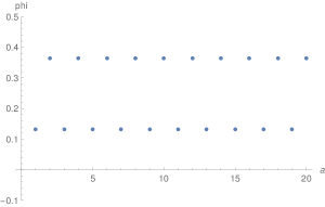
The following numerical results support the qualitative discussion above. In fact, the actual phase structure is more complex than that. We have considered some fixed values of $N,\ \kappa$ and have gone through discrete values of $\xi$ with small intervals. For every $\xi$, a numerical search for the global minimum of the free energy has been performed, and the minimum value is plotted. The result for $N=20,\ \kappa=1$ is shown in the left figure of Fig. 6. We also evaluate the first derivative of the free energy with respect to $\xi$ by taking the finite differentials of these data, and the result is plotted in the right figure of Fig. 6. On the other hand, the free energy of the flat space can be computed analytically by using the results in Section 4, and is plotted by the dotted lines for the comparison. If a data point is apart from the dotted lines, it is in a phase different from the flat space. From these figures, we can see that there seem to exist four phases, and we label them by their regions: (i) $\xi\gtrsim 0.12$, (ii) $-0.1\lesssim\xi\lesssim 0.12$, (iii)$-0.14\lesssim\xi\lesssim-0.1$, (iv) $\xi\lesssim-0.14$. From the right figure, one can see that the phase transitions between (i) and (ii) and between (ii) and (iii) are first-order (the former is much weaker), while that between (iii) and (iv) is second-order.

Figure 6: The left: the free energy for $N=20,\ \kappa=1$. The horizontal and vertical axes represent $\xi$ and the free energy, respectively. The right: the first derivative of the free energy obtained by taking the finite differentials of the data in the left figure. In the two figures, the dotted lines represent the free energy and its first derivative of the flat space.

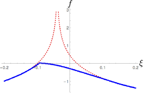
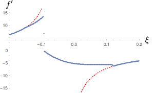
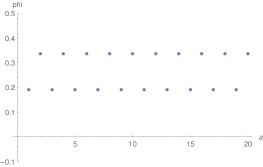
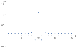
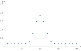
In the phase (i) and (iv), ${\bar{\phi}}$ takes the constant value $\sqrt{\frac{3}{2N}}$, and they represent the flat space in Section 4. They are certainly in the regions with large $|\xi|$, which is consistent with the qualitative discussion above. As can be seen in the left figure of Fig. 7, in the phase (ii), ${\bar{\phi}}$ takes non-zero values only around a certain point ($a\sim 10$ in the figure). This is the phase of a point-like space discussed above. Because $P$ is invariant under the discrete translation $a\rightarrow a+l\,{\rm mod}\,N$ with arbitrary integers $l$, the location of the central point is arbitrary. This is a phase where the discrete translation symmetry is all broken, since ${\bar{\phi}}_{a}\neq{\bar{\phi}}_{a+l\,{\rm mod}\,N}$. On the other hand, the right figure of Fig. 7 shows that, in the phase (iii), ${\bar{\phi}}$ oscillates with period 2. Therefore, ${\bar{\phi}}$ remains invariant under the even translations, ${\bar{\phi}}_{a}={\bar{\phi}}_{a+2l\,{\rm mod}\,N}$, and this is a phase where the discrete translation symmetry is only partially broken. The second order of the phase transition between (iii) and (iv) suggests that the transition is triggered by a negative eigenvalue. In fact, from the result of Section 4, one can easily get that this is triggered by the change of the sign of the eigenvalue of the mode with $n=\frac{N}{2}$. The mode is an oscillatory mode with period 2, and the oscillatory profile of ${\bar{\phi}}$ in the phase (iii) is explained by the condensation of the mode.

Figure 7: The configurations of ${\bar{\phi}}$ in the phase (ii) ($\xi=0$) and (iii) ($\xi=-0.12$) for $N=20,\ \kappa=1$ are plotted in the left and right figures, respectively. The vertical and horizontal axes represent the values of ${\bar{\phi}}_{a}$ and the index $a$, respectively.

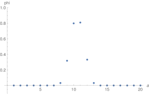
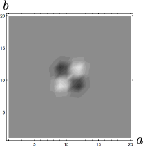
Let us explain the reason why the phase (ii) represents a point-like space. One reason is that ${\bar{\phi}}$ takes non-vanishing values only in a small point-like region, as around $a\sim 10$ in the left figure of Fig. 7. A physically more convincing explanation is that the correlation function takes non-vanishing values only in the vicinity of the non-vanishing region of ${\bar{\phi}}$. Fig. 8 plots the two-point correlation function for the phase (ii) ($\xi=0,\ N=20,\ \kappa=1$) for the case of ${\bar{\phi}}$ in the left figure of Fig. 7.

Figure 8: The contour plot of the connected two-point function $\langle\varphi_{a}\varphi_{b}\rangle_{\text{con.}}$ for $N=20,\ \kappa=1,\ \xi=0$, corresponding to the case with ${\bar{\phi}}$ in the left figure of Fig. 7. The white and black regions represent positive and negative values, respectively, while the gray region represents vanishing values. Thus, in the point-like space, the non-vanishing values of the correlation function are concentrated only around $a,b\sim 10$, namely the non-vanishing region of $\bar{\phi}$.

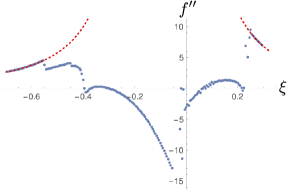
The phase depends on $N$ and $\kappa$ as well. The dependence does not seem simple, and some systematic studies seem to be required to obtain a convincing picture. Here, we just give another example for $N=20,\ \kappa=-1$ in Fig. 9. These figures respectively show the first and second derivatives of the free energy with respect to $\xi$, which are obtained by finite differentiations as in the previous example. There seem to exist more phases than the previous case with $\kappa=1$.

Figure 9: The first (left) and second (right) derivatives of the free energy for $N=20,\ \kappa=-1$. The horizontal axis represents $\xi$. The dotted lines represent the case of the flat space. There seem to exist two first order phase transitions at the similar locations as in the previous case with $\kappa=1$, while there seem to exist more second order transitions.

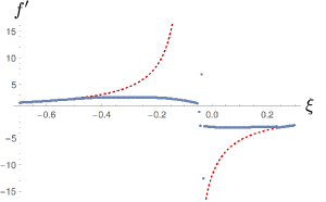
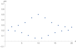
In Fig. 10, the profiles of ${\bar{\phi}}$ for four values of $\xi$ are shown (The flat cases are not shown, since they are just constant). The down-right figure corresponds to the point-like space. The $\bar{\phi}$ in the first two figures are consistent with the picture that, as $\xi$ is increased from a large negative value, two second order phase transitions triggered by negative eigenvalues occur successively. The first one is a condensation of a mode with an oscillation period 2, and the second one of another mode with another frequency.

Figure 10: The profiles of ${\bar{\phi}}$ for four values of $\xi$ with $N=20,\ \kappa=-1$. The up-left figure is for $\xi=-0.5$, the up-right for $\xi=-0.42$, the down-left for $\xi=-0.2$, and the down-right for $\xi=0.1$, respectively.

7 Summary and discussions

In this paper, we have shown that classical spaces with geometries, generally curved, in arbitrary dimensions can be generated on boundaries of randomly connected tensor networks in the thermodynamic limit by appropriately choosing the tensors. In particular, we have seen that such a tensor must contain not only a local part representing structures of local neighbourhoods but also a non-local part which stabilizes the space. The non-local part does not cause problems of non-locality in the emergent space, since it affects only a single global mode and cannot be detected by a local observer in the large $N$ limit. We have given the explicit solvable examples of arbitrary dimensional flat tori. As for the general case, the correspondence from the tensor to the geometry of the emergent space has been obtained from an analysis of an effective action. The action has an invariant form under the spatial diffeomorphism, which is an outcome of the underlying orthogonal group symmetry of the randomly connected tensor network. We have also studied phase transitions among various kinds of spaces including extended and point-like ones.

In the randomly connected tensor network, the tensor is a given external variable rather than a dynamical one, and therefore the emergent space is a static object. This is an unsatisfactory situation from the perspective of quantum gravity and even in classical contexts. On the other hand, the tensor is a dynamical variable in the canonical tensor model (CTM), and its Hamiltonian generates a flow equation for the tensor of the randomly connected tensor network, which can be regarded as a renormalization group flow [19, 20]. Then, by using the result of this paper about the correspondence from the tensor to the geometry, the dynamical equation of CTM can be translated to a dynamical equation for the geometry of the emergent space. The form of the latter equation would be highly interesting to study, since CTM is known to have intimate connections to general relativity [15, 16]. It would also be interesting to see whether the tensors generating extended spaces are dynamically favoured or not, since quantum gravity should provide some explanations for our actual spacetime.

Interestingly, the non-local part of the tensor has precisely the form which is equivalent to an addition of a negative cosmological constant in the framework of CTM [21]. Then the two main implications of this paper, emergent spaces on boundaries and necessity of negative cosmological constants for stability, curiously resembles a part of the AdS/CFT correspondence [41] in string theory. It has also been argued that the tensor networks (though not random) are discrete realizations of the AdS spaces [42]. Showing any connections between our framework and the AdS/CFT correspondence is presently far beyond our scope, but the resemblance would at least suggest an interesting direction of study: not only boundaries, but random networks themselves may also have effective geometries, as the bulk geometries of the AdS spaces. This contradicts the difficulties mentioned in Section 3, but there would remain the possibility that such classical geometries on randomly connected tensor networks would appear in certain sophisticated limits of the parameters, as the bulk geometries of AdS in string theory have definite meanings only in semi-classical limits.

Obviously, putting matters on the emergent space would also be an interesting direction of study. This would be possible by considering tensors more complex than this paper, and the super-extension discussed in [43].

Acknowledgements

The work of N.S. is supported in part by JSPS KAKENHI Grant Number 15K05050. The work of Y.S. is funded under CUniverse research promotion project by Chulalongkorn University (grant reference CUAASC).

Appendix A Notes on covariance

As mentioned in Section 5, in this appendix, we will show the linear relation between the moments and the covariant moments defined by (57) and (59), respectively. This ensures that the two ways of description are equivalent within the order we are considering. In order to show this, note that the test functions, $f_{1}$, $f_{2}$ and $f_{3}$, defined in (57) and (59) should transform as scalar half-densities under the spatial diffeomorphism [16]. Thus we can parametrise the test functions in terms of scalars, $s_{1}$, $s_{2}$ and $s_{3}$, as

$$f_{1}=g^{1/4}s_{1},\ \ \ f_{2}=g^{1/4}s_{2},\ \ \ f_{3}=g^{1/4}s_{3}.$$ (71)

Plugging (71) into (57) and (59) and comparing the coefficients of $s_{1}s_{2}s_{3}$, $s_{1}\partial_{\mu}(s_{2}s_{3})$, $s_{1}\partial_{\mu}s_{2}\partial_{\nu}s_{3}$, and $s_{1}(\partial_{\mu}\partial_{\nu}s_{2})s_{3}+s_{1}s_{2}(\partial_{\mu}\partial_{\nu}s_{3})$, respectively, we can obtain the relation between the moments and the covariant moments as

$$\alpha_{c}=\alpha+\frac{1}{2}\beta^{\mu}g_{\mu}+\frac{1}{4}\gamma^{\mu\nu}\left(\partial_{\mu}g_{\nu}+\frac{1}{4}g_{\mu}g_{\nu}\right)+\frac{1}{16}\tilde{\gamma}^{\mu\nu}g_{\mu}g_{\nu}+\cdots,$$ (72)

$$\beta^{\mu}_{c}-\frac{1}{2}\gamma_{c}^{\nu\rho}\Gamma_{\nu\rho}^{\mu}=\beta^{\mu}+\frac{1}{4}\gamma^{\mu\nu}g_{\nu}+\frac{1}{4}\tilde{\gamma}^{\mu\nu}g_{\nu}+\cdots,$$ (73)

$$\gamma^{\mu\nu}_{c}=\gamma^{\mu\nu}+\cdots,$$ (74)

$$\tilde{\gamma}^{\mu\nu}_{c}=\tilde{\gamma}^{\mu\nu}+\cdots,$$ (75)

where $\Gamma^{\mu}_{\nu\rho}$ is the Christoffel symbol associated with $g_{\mu\nu}$, the dots represent the higher order corrections neglected in the analysis and

$$g_{\mu}:=g^{\lambda\tau}\partial_{\mu}g_{\lambda\tau}.$$ (76)

References

- [1] J. Ambjorn, B. Durhuus and T. Jonsson, “Three-Dimensional Simplicial Quantum Gravity And Generalized Matrix Models,” Mod. Phys. Lett. A 6, 1133 (1991).
- [2] N. Sasakura, “Tensor Model For Gravity And Orientability Of Manifold,” Mod. Phys. Lett. A 6, 2613 (1991).
- [3] N. Godfrey and M. Gross, “Simplicial Quantum Gravity In More Than Two-Dimensions,” Phys. Rev. D 43, 1749 (1991).
- [4] M. Fukuma, S. Sugishita and N. Umeda, “Random volumes from matrices,” JHEP 1507, 088 (2015) doi:10.1007/JHEP07(2015)088 [arXiv:1503.08812 [hep-th]].
- [5] M. Fukuma, S. Sugishita and N. Umeda, “Putting matters on the triangle-hinge models,” arXiv:1504.03532 [hep-th].
- [6] R. Gurau, “Colored Group Field Theory,” Commun. Math. Phys. 304, 69 (2011) [arXiv:0907.2582 [hep-th]].
- [7] R. Gurau and J. P. Ryan, “Colored Tensor Models - a review,” SIGMA 8, 020 (2012) [arXiv:1109.4812 [hep-th]].
- [8] V. Bonzom, R. Gurau, A. Riello and V. Rivasseau, “Critical behavior of colored tensor models in the large N limit,” Nucl. Phys. B 853, 174 (2011) [arXiv:1105.3122 [hep-th]].
- [9] R. Gurau and J. P. Ryan, “Melons are branched polymers,” Annales Henri Poincare 15, no. 11, 2085 (2014) [arXiv:1302.4386 [math-ph]].
- [10] J. Ambjorn, J. Jurkiewicz and R. Loll, “Emergence of a 4-D world from causal quantum gravity,” Phys. Rev. Lett. 93 (2004) 131301 [hep-th/0404156].
- [11] S. Horata, H. S. Egawa, N. Tsuda and T. Yukawa, “Phase structure of four-dimensional simplicial quantum gravity with a U(1) gauge field,” Prog. Theor. Phys. 106 (2001) 1037 [hep-lat/0004021].
- [12] J. Ambjorn, K. N. Anagnostopoulos and J. Jurkiewicz, “Abelian gauge fields coupled to simplicial quantum gravity,” JHEP 9908 (1999) 016 [hep-lat/9907027].
- [13] N. Sasakura, “Canonical tensor models with local time,” Int. J. Mod. Phys. A 27, 1250020 (2012) doi:10.1142/S0217751X12500200 [arXiv:1111.2790 [hep-th]].
- [14] N. Sasakura, “Uniqueness of canonical tensor model with local time,” Int. J. Mod. Phys. A 27, 1250096 (2012) doi:10.1142/S0217751X12500960 [arXiv:1203.0421 [hep-th]].
- [15] N. Sasakura and Y. Sato, “Interpreting canonical tensor model in minisuperspace,” Phys. Lett. B 732, 32 (2014) doi:10.1016/j.physletb.2014.03.006 [arXiv:1401.2062 [hep-th]].
- [16] N. Sasakura and Y. Sato, “Constraint algebra of general relativity from a formal continuum limit of canonical tensor model,” JHEP 1510 (2015) 109 doi:10.1007/JHEP10(2015)109 [arXiv:1506.04872 [hep-th]].
- [17] S. N. Dorogovtsev, A. V. Goltsev and J. F. F. Mendes, “Critical phenomena in complex networks,” Rev. Mod. Phys. 80, 1275 (2008).
- [18] N. Sasakura and Y. Sato, “Exact Free Energies of Statistical Systems on Random Networks,” SIGMA 10, 087 (2014) [arXiv:1402.0740 [hep-th]].
- [19] N. Sasakura and Y. Sato, “Ising model on random networks and the canonical tensor model,” PTEP 2014, no. 5, 053B03 (2014) [arXiv:1401.7806 [hep-th]].
- [20] N. Sasakura and Y. Sato, “Renormalization procedure for random tensor networks and the canonical tensor model,” PTEP 2015, no. 4, 043B09 (2015) [arXiv:1501.05078 [hep-th]].
- [21] G. Narain, N. Sasakura and Y. Sato, “Physical states in the canonical tensor model from the perspective of random tensor networks,” JHEP 1501, 010 (2015) doi:10.1007/JHEP01(2015)010 [arXiv:1410.2683 [hep-th]].
- [22] N. Sasakura, “Quantum canonical tensor model and an exact wave function,” Int. J. Mod. Phys. A 28, 1350111 (2013) doi:10.1142/S0217751X1350111X [arXiv:1305.6389 [hep-th]].
- [23] R. Penrose, “Angular momentum: An approach to combinatorial spacetime,” in Quantum Theory and Beyond, Cambridge Univ. Press (1971).
- [24] C. Rovelli and F. Vidotto, “Covariant Loop Quantum Gravity : An Elementary Introduction to Quantum Gravity and Spinfoam Theory,” Cambridge Univ. Press (2014).
- [25] L. Bombelli, J. Lee, D. Meyer, and R. D. Sorkin, “Space-time as a causal set,” Phys. Rev. Lett. 59 (1987), 521.
- [26] D. P. Rideout and R. D. Sorkin, “Classical sequential growth dynamics for causal sets,” Phys. Rev. D 61 (1999) 024002.
- [27] M. Cortês and L. Smolin, “The Universe as a Process of Unique Events,” Phys. Rev. D 90 (2014) 8, 084007 doi:10.1103/PhysRevD.90.084007 [arXiv:1307.6167 [gr-qc]].
- [28] M. Cortês and L. Smolin, “Quantum energetic causal sets,” Phys. Rev. D 90 (2014) 4, 044035 doi:10.1103/PhysRevD.90.044035 [arXiv:1308.2206 [gr-qc]].
- [29] T. Konopka, F. Markopoulou and L. Smolin, “Quantum Graphity,” hep-th/0611197.
- [30] T. Konopka, F. Markopoulou and S. Severini, “Quantum Graphity: A Model of emergent locality,” Phys. Rev. D 77 (2008) 104029 doi:10.1103/PhysRevD.77.104029 [arXiv:0801.0861 [hep-th]].
- [31] A. Hamma, F. Markopoulou, S. Lloyd, F. Caravelli, S. Severini and K. Markstrom, “A Quantum Bose-Hubbard model with evolving graph as toy model for emergent spacetime,” Phys. Rev. D 81 (2010) 104032 doi:10.1103/PhysRevD.81.104032 [arXiv:0911.5075 [gr-qc]].
- [32] C. A. Trugenberger, “Quantum Gravity as an Information Network: Self-Organization of a 4D Universe,” Phys. Rev. D 92 (2015) 084014 doi:10.1103/PhysRevD.92.084014 [arXiv:1501.01408 [hep-th]].
-
[33]
C. A. Trugenberger,
“Critical Space-Time Networks and Geometric Phase Transitions from Frustrated Edge Antiferromagnetism,”
Phys. Rev. E 92 (2015) 6, 062818
doi:10.1103/PhysRevE.92.062818 [arXiv:1507.01820 [hep-th]]. - [34] S. Wolfram, “A new kind of science,” Wolfram Media (2002) 1197pp, ISBN 1-57955-008-8.
- [35] G. M. D’Ariano and A. Tosini, “Space-time and special relativity from causal networks,” arXiv:1008.4805 [gr-qc].
- [36] M. Requardt and S. Rastgoo, “The Structurally Dynamic Cellular Network and Quantum Graphity Approaches to Quantum Gravity and Quantum Geometry - A Review and Comparison,” J. Cell. Automata 10 (2015) 5-6, 341 [arXiv:1501.00391 [gr-qc]].
- [37] M. Requardt, “Scale free small world networks and the structure of quantum space-time,” gr-qc/0308089.
- [38] G. Bianconi, C. Rahmede and Z. Wu, “Complex Quantum Network Geometries: Evolution and Phase Transitions,” Phys. Rev. E 92 (2015) 2, 022815 doi:10.1103/PhysRevE.92.022815 [arXiv:1503.04739 [cond-mat.dis-nn]].
- [39] G. Bianconi and C. Rahmede, “Complex Quantum Network Manifolds in Dimension are Scale-Free,” Sci. Rep. 5 (2015) 13979 doi:10.1038/srep13979 [arXiv:1506.02648 [gr-qc]].
- [40] G. Bianconi and C. Rahmede, “Network geometry with flavor: from complexity to quantum geometry,” arXiv:1511.04539 [cond-mat.stat-mech].
- [41] J. M. Maldacena, “The Large N limit of superconformal field theories and supergravity,” Int. J. Theor. Phys. 38, 1113 (1999) [Adv. Theor. Math. Phys. 2, 231 (1998)] doi:10.1023/A:1026654312961 [hep-th/9711200].
- [42] B. Swingle, “Entanglement Renormalization and Holography,” Phys. Rev. D 86, 065007 (2012) doi:10.1103/PhysRevD.86.065007 [arXiv:0905.1317 [cond-mat.str-el]].
- [43] G. Narain and N. Sasakura, “An OSp extension of the canonical tensor model,” PTEP 2015, no. 12, 123A05 (2015) doi:10.1093/ptep/ptv169 [arXiv:1509.01432 [hep-th]].