Multipolar third-harmonic generation driven by optically-induced magnetic resonances

Abstract

We analyze third-harmonic generation from high-index dielectric nanoparticles and discuss the basic features and multipolar nature of the parametrically generated electromagnetic fields near the Mie-type optical resonances. By combining both analytical and numerical methods, we study the nonlinear scattering from simple nanoparticle geometries such as spheres and disks in the vicinity of the magnetic dipole resonance. We reveal the approaches for manipulating and directing the resonantly enhanced nonlinear emission with subwavelength all-dielectric structures that can be of a particular interest for novel designs of nonlinear optical antennas and engineering the magnetic optical nonlinear response at nanoscale.

The pursuit for using all-dielectric components as building blocks in nanoscale devices and photonic circuitry constitutes an important trend in modern nanophotonics Jahani and Jacob (2016). It ultimately aims to circumvent the challenge of Ohmic losses and heating detrimental to the performance of conventional metal-based plasmonics. Nanostructures made of high-refractive-index semiconductors and dielectrics exhibit strong interaction with light due to the excitation of the localized Mie-type resonances they sustain Garcia-Etxarri et al. (2011); Schmidt et al. (2012). Shrinking light in high-index and low-loss dielectric nanoparticles, acting as open optical high-$Q$ resonators (or resonant optical nanoantennas), opens up an access to the optically-induced response of magnetic nature associated with magnetic field multipoles. In most previous works on trapped magnetic resonances, silicon was the primary focus of the material Evlyukhin et al. (2012); Kuznetsov et al. (2012); Staude et al. (2013); Zywietz et al. (2014); Liu et al. (2014a); Zywietz et al. (2015). Remarkably, along with a moderately high refractive index and relatively low absorption at the visible, infrared and telecom frequencies Palik (1985), silicon, both crystalline and amorphous, possesses a strong cubic optical nonlinearity Burns and Bloembergen (1971); Moss et al. (1989, 1990); Bristow et al. (2007); Lin et al. (2007); Zhang et al. (2007); Ikeda et al. (2007); Vivien and Pavesi (2013); Gai et al. (2014) that makes it suitable for all-dielectric nonlinear nanophotonics, bringing many intriguing capabilities of the efficient all-optical light control. Recently, the enhancement of nonlinear response attributed to the magnetic dipole resonances in silicon nanodisks has been demonstrated experimentally Shcherbakov et al. (2014, 2015a, 2015b).

Generally, in the problems of both linear and nonlinear scattering at arbitrary nanoscale objects, multipole decomposition of the scattered electromagnetic fields (see METHODS) provides a transparent interpretation for the measurable far-field characteristics, such as radiation efficiency and radiation patterns, since they are essentially determined by the interference of dominating excited multipole modes Jackson (1965); Bohren and Huffman (1983); Dadap et al. (1999, 2004); Kujala et al. (2008); Petschulat et al. (2009); Gonella and Dai (2011); Mühlig et al. (2011); Huttunen et al. (2012); Capretti et al. (2012); Grahn et al. (2012). Tuning the contributions of different-order multipole moments is used to engineer the scattering and tailor the emission directionality of optical nanoantennas Liu et al. (2012); Rodrigo et al. (2013); Staude et al. (2013); Fu et al. (2013); Poutrina et al. (2013); Krasnok et al. (2014a); Smirnova et al. (2014); Davidson II et al. (2015); Dregely et al. (2014); Liberal et al. (2015). In particular, the first Kerker condition for overlapped and balanced electric and magnetic dipoles represents an example for zero backscattering Kerker et al. (1983). Developing this concept, the directionality of the scattering can be improved through the interference of properly excited higher-order electric and magnetic modes Liu et al. (2014b); Hancu et al. (2014); Naraghi et al. (2015); Alaee et al. (2015). Given the fact that considerable electromagnetic energy can be confined to small volumes in nanostructured materials, nonlinear optical phenomena are of a special interest, and they offer exclusive prospects for engineering fast and strong optical nonlinearity and controlling light by light. By virtue of subwavelength localization of eigenmodes and resonant character of their excitation, nonlinear effects may become quite pronounced, even at relatively weak external fields Kauranen and Zayats (2012). Therefore, nonlinear response depends largely on localized resonant effects in nanostructures, allowing for nonlinear optical components to be scaled down in size, which is important for fully functional photonic circuitry.

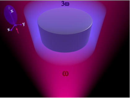
Figure 1: Schematic of the third-harmonic generation from a resonant nanoparticle. A dielectric nanodisk is illuminated by laser light from the bottom. The third-harmonic radiation is shown predominantly emitted into the upper half-space, with a forward-directed radiation pattern formed in the far-field, when the magnetic and electric dipolar modes overlap at the fundamental frequency under the plane wave excitation.

The efficiency of harmonic generation can be strongly enhanced in nanostructures, provided the pump or generated frequency matches the supported resonance Boyd (2008), especially, if the geometry is doubly resonant Hayat and Orenstein (2007); Banaee and Crozier (2011); Thyagarajan et al. (2012); Navarro-Cia and Maier (2012); Aouani et al. (2012); Ginzburg et al. (2012), i.e. sustains resonances at both the fundamental and harmonic frequencies, and spatial distribution of the nonlinear source is such that it strongly couples the corresponding modes. In this respect, electric dipolar resonance has been widely exploited in deeply subwavelength metallic particles and their composites, and thereby plasmonic nanostructures offer a unique playground to study a rich diversity of nonlinear phenomena, including second-harmonic generation (SHG) Roke and Gonella (2012); Kauranen and Zayats (2012); Butet et al. (2015); Segovia et al. (2015), third-harmonic generation (THG) Metzger et al. (2012); Hentschel et al. (2012); Metzger et al. (2014) and four-wave mixing (FWM) Zhang et al. (2013). To characterize the nonlinear scattering, the nonlinear Mie theory was developed over recent decades Dewitz et al. (1996); Pavlyukh and Hübner (2004); de Beer and Roke (2009); Gonella and Dai (2011); Butet et al. (2012); Roke and Gonella (2012) as an extension of the analytical approach outlined in Refs. Dadap et al. (1999, 2004) for the Rayleigh limit of SHG from a spherical particle. This theory can be applied to metallic nanoparticles to describe SHG governed by the dominant surface SH polarization source Bachelier et al. (2010); Wang et al. (2009).

In the case of metamaterials, specific nonlinear regimes can be achieved due to magnetic optical response of ”meta-atoms” Shadrivov et al. (2015); Rose et al. (2013); Kruk et al. (2015). Alternatively to lossy metal-based setups constructed to support loop currents, high-index dielectric particles can present a strong magnetic response and demonstrate magnetic properties associated with Mie resonances. In this way, resonantly enhanced nonlinear effects for nonlinear dielectric particles of sizes comparable with the inner wavelength are expected around the frequencies of Mie modes.

The main purpose of this paper is twofold. First, we discuss the key theoretical aspects underlying the third-harmonic generation from high-index dielectric nanoparticles excited near the magnetic dipole resonance (see Fig. 1) by applying the analytical approach and confirming the analytical predictions by the full-scale numerical simulations in the case of simple geometries such as spheres and disks. Second, we reveal the basic mechanisms for manipulating and directing nonlinear scattering with all-dielectric structures that can be of a particular interest for novel designs of nonlinear optical antennas Bharadwaj et al. (2009); Novotny and van Hulst (2011); Krasnok et al. (2013, 2014b).

RESULTS AND DISCUSSIONS

Third-harmonic generation from a spherical nanoparticle

To gain physical insight, we start with developing the basic analytical tools of the third-harmonic generation, and consider a high-permittivity spherical dielectric particle of radius $a$ and linear refractive index $n$, placed in homogeneous space and excited by the linearly-polarized plane wave propagating in the $z$ direction, ${\bf E}_{i}({\bf r})=\hat{{\bf x}}E_{0}e^{ik_{1}z}$. The interior of the sphere and exterior region are characterized by the permittivities $\varepsilon_{2}$ and $\varepsilon_{1}$, and permeabilities $\mu_{2}$ and $\mu_{1}$, respectively. For conceptual clarity, we assume that the materials are nonmagnetic, i.e. $\mu_{2}=\mu_{1}=\mu_{0}$, isotropic and lossless. The particle possesses the third-order nonlinearity, bulk and isotropic, and its nonlinear response is described by the nonlinear polarization ${\bf P}^{(3)}=\varepsilon_{0}\chi^{(3)}_{V}{\bf E}^{3}$, induced by the pump field, where $\chi^{(3)}_{V}$ is the cubic susceptibility.

The problem of linear light scattering by a sphere is solved using the multipole expansion, well-known as Mie theory Bohren and Huffman (1983); Jackson (1965). In accord with the exact Mie solution, the linear scattering spectum features resonances accompanied by the local field enhancement. If the refractive index is high enough, electric (ED) and magnetic (MD) dipolar resonances are well-separated in frequency and rather narrow (we illustrate this case for an example of large $n$ in Fig. S1(a) of Supporting Information), and the electric field profiles within the particle at the resonances are substantially different. The structure of the local fields is known to play an indefeasible role in nonlinear optical effects with both dielectric and plasmonic resonant systems. In the vicinity of resonances, the field distribution inside the particle excited by the plane wave can be approximated by the corresponding specific eigenmode. Here, we focus on the MD resonance, exhibiting a higher quality factor, and elaborate a fully analytical treatment of the nonlinear problem.

In the single MD mode approximation, the electric field inside the particle at $r<a$ is expressed as

$$\begin{split}{\bf{E}}^{\text{in}}\left({\omega}\right)\approx&{E_{0}}{{{A^{\text{in}}_{M}(1,1)j_{1}(k_{2}(\omega)r)\left\{{\bf{X}}_{1,1}({\theta,\varphi})+{\bf{X}}_{1,-1}({\theta,\varphi})\right\}}}}\\ =&A(\omega)j_{1}(k_{2}(\omega)r)\left\{\bm{\hat{\theta}}\cos\varphi-\sin\varphi\cos\theta\bm{\hat{\varphi}}\right\},\end{split}$$ (1)

where $k_{2}(\omega)=\omega\sqrt{\varepsilon_{2}(\omega)\mu_{2}}=k_{0}\sqrt{\varepsilon_{2r}{\mu_{2r}}}$ is the wavenumber inside the sphere, $j_{1}(k_{2}(\omega)r)$ is the spherical Bessel function of the first order, ${\bf{X}}_{1,1}({\theta,\varphi})=\displaystyle\frac{1}{4}\sqrt{\displaystyle\frac{3}{\pi}}\{0,1,i\cos{\theta}\}\text{exp}(i\varphi)$ is the vector spherical harmonic of degree $l=1$ and order $m=1$, $A(\omega)=E_{0}A^{\text{in}}_{M}(1,1)\displaystyle\frac{1}{2}\sqrt{\displaystyle\frac{3}{\pi}}$, coefficient $A^{\text{in}}_{M}(1,1)$ is known from Mie theory Bohren and Huffman (1983); Jackson (1965). For convenience, we rewrite Eq. (1) in the spherical coordinate system associated with $y$ axis [$z^{\prime}\leftrightarrow y$, codirected with the magnetic field in the incident plane wave, as shown in Fig. 2(a)]

$${\bf{E}}^{\text{in}}\left({\omega}\right)\approx A(\omega)j_{1}(k_{2}(\omega)r)\sin{\theta^{\prime}}\bm{\hat{\varphi^{\prime}}}.$$ (2)

In what follows, performing a multipole expansion of the numerically computed fields, the multipole moments are calculated in the prime spherical coordinates.

Since the nonlinear medium is isotropic, the nonlinear volume current density induced in the particle at the tripled frequency $3\omega$ is azimuthal, akin to the electric field, ${\bf j}^{(3\omega)}=-3i\omega{\bf{P}}^{\left({3\omega}\right)}$, where ${\bf{P}}^{(3\omega)}=\varepsilon_{0}\chi^{(3)}_{V}(E^{\text{in}}_{\varphi^{\prime}}(\omega))^{3}\bm{\hat{\varphi^{\prime}}}$:

$${\bf j}^{(3\omega)}=-i3\omega\varepsilon_{0}\chi^{(3)}_{V}A^{3}(\omega)j^{3}_{1}(k_{2}(\omega)r)\sin^{3}{\theta^{\prime}}\bm{\hat{\varphi^{\prime}}}\>.$$ (3)

Looking for the solution of Maxwell’s equations written for the region $r<a$ with this source in the right-hand side

$$\begin{cases}\nabla\times{\bf E}_{(3\omega)}=3i\omega\mu_{2}{\bf H}_{(3\omega)},&\\ \nabla\times{\bf H}_{(3\omega)}=-3i\omega\varepsilon_{2}(3\omega){\bf E}_{(3\omega)}+{\bf j}^{(3\omega)}\end{cases}$$ (4)

in the form ${\bf E}_{(3\omega)}={E}_{(3\omega)}(r,\theta^{\prime})\bm{\hat{\varphi^{\prime}}}$, we obtain the equation

$$\nabla\times\nabla\times{\bf E}_{(3\omega)}-9\omega^{2}\varepsilon_{2}(3\omega)\mu_{2}{\bf E}_{(3\omega)}={f}(r)\sin^{3}{\theta^{\prime}}\bm{\hat{\varphi^{\prime}}}\>,$$ (5)

where ${f}(r)=9\omega^{2}\mu_{2}\varepsilon_{0}\chi^{(3)}_{V}A^{3}(\omega)j^{3}_{1}(k_{2}(\omega)r)$. Accomplishing the vector operations, we get the following scalar equation to solve:

$$\frac{\partial^{2}}{\partial r^{2}}E_{(3\omega)}+\displaystyle\frac{2}{r}\displaystyle\frac{\partial}{\partial r}E_{(3\omega)}+\displaystyle\frac{1}{r^{2}}\displaystyle\frac{\partial}{\partial\theta^{\prime}}\displaystyle\frac{1}{\sin\theta^{\prime}}\displaystyle\frac{\partial}{\partial\theta^{\prime}}\sin{\theta^{\prime}}E_{(3\omega)}+9\omega^{2}\varepsilon_{2}(3\omega)\mu_{2}{E}_{(3\omega)}=-{f}(r)\sin^{3}{\theta^{\prime}}\>.$$ (6)

Homogeneous Eq. (6) possesses solutions of the form $R_{l}(3\omega\sqrt{\varepsilon_{2}(3\omega)\mu_{2}}r)\displaystyle\frac{d\mathcal{Y}_{l0}(\theta^{\prime})}{d\theta^{\prime}}$, where the functions $R_{l}$ and $\mathcal{Y}_{l0}$ satisfy

$$\frac{d^{2}R_{l}}{dr^{2}}+\frac{2}{r}\frac{dR_{l}}{dr}+\left(9\omega^{2}\varepsilon_{2}(3\omega)\mu_{2}-\frac{l(l+1)}{r^{2}}\right)R_{l}=0\>,$$ (7)

$$\frac{1}{\sin\theta^{\prime}}\frac{d}{d\theta^{\prime}}{\sin\theta^{\prime}}\frac{d\mathcal{Y}_{l0}}{d\theta^{\prime}}+l(l+1)\mathcal{Y}_{l0}=0\>,$$

and the angular functions $\mathcal{Y}_{l0}$ and their derivatives up to $l=3$ are written as

$$\mathcal{Y}_{10}=\sqrt{\displaystyle\frac{3}{4\pi}}\cos{\theta^{\prime}}\>,\quad\frac{d\mathcal{Y}_{10}}{d\theta^{\prime}}=-\sqrt{\displaystyle\frac{3}{4\pi}}\sin{\theta^{\prime}},\>$$ (8)

$$\mathcal{Y}_{20}=\sqrt{\displaystyle\frac{5}{4\pi}}\left(\frac{3}{2}\cos^{2}{\theta^{\prime}}-\frac{1}{2}\right)\>,\quad\frac{d\mathcal{Y}_{20}}{d\theta^{\prime}}=-\sqrt{\displaystyle\frac{5}{4\pi}}\frac{3}{2}\sin{2\theta^{\prime}},\>$$

$$\mathcal{Y}_{30}=\sqrt{\displaystyle\frac{7}{4\pi}}\left(\frac{5}{2}\cos^{3}{\theta^{\prime}}-\frac{3}{2}\cos{\theta^{\prime}}\right)\>,\quad\frac{d\mathcal{Y}_{30}}{d\theta^{\prime}}=\sqrt{\displaystyle\frac{7}{4\pi}}\frac{15}{2}\left(\sin^{3}{\theta^{\prime}}-\frac{4}{5}\sin{\theta^{\prime}}\right)\>.$$

The angular-dependent part of the source in Eq. (6) can be represented as $\sin^{3}{\theta^{\prime}}=\displaystyle\frac{2}{15}\sqrt{\displaystyle\frac{4\pi}{7}}\displaystyle\frac{d\mathcal{Y}_{30}}{d\theta^{\prime}}-\displaystyle\frac{4}{5}\sqrt{\displaystyle\frac{4\pi}{3}}\displaystyle\frac{d\mathcal{Y}_{10}}{d\theta^{\prime}}$. Thereby, the solution of Eq. (6) are sought using separation of variables in the form

$$E_{(3\omega)}=\mathcal{E}^{(1)}_{3\omega}(r)\displaystyle\frac{d\mathcal{Y}_{10}}{d\theta^{\prime}}+\mathcal{E}^{(3)}_{3\omega}(r)\displaystyle\frac{d\mathcal{Y}_{30}}{d\theta^{\prime}},$$ (9)

where two terms correspond to the magnetic dipole (MD) and magnetic octupole (MO) excitations, and for the radial functions we have inhomogeneous equations

$$\frac{d^{2}\mathcal{E}^{(1)}_{3\omega}}{dr^{2}}+\frac{2}{r}\frac{d\mathcal{E}^{(1)}_{3\omega}}{dr}+\left(9\omega^{2}\varepsilon_{2}(3\omega)\mu_{2}-\frac{2}{r^{2}}\right)\mathcal{E}^{(1)}_{3\omega}=\frac{4}{5}\sqrt{\displaystyle\frac{4\pi}{3}}{f}(r)\equiv{f}^{(1)}(r),\>$$ (10)

$$\frac{d^{2}\mathcal{E}^{(3)}_{3\omega}}{dr^{2}}+\frac{2}{r}\frac{d\mathcal{E}^{(3)}_{3\omega}}{dr}+\left(9\omega^{2}\varepsilon_{2}(3\omega)\mu_{2}-\frac{12}{r^{2}}\right)\mathcal{E}^{(3)}_{3\omega}=-\frac{2}{15}\sqrt{\displaystyle\frac{4\pi}{7}}{f}(r)\equiv{f}^{(3)}(r)\>.$$

Matching the fields at the spherical particle surface $r=a$ by imposing boundary conditions of continuity for the tangential field components $E_{{\varphi^{\prime}}(3\omega)}(r,\theta^{\prime})$ and $H_{{\theta^{\prime}}(3\omega)}\propto\displaystyle\frac{1}{r}\left[-\displaystyle\frac{\partial}{\partial r}\left(rE_{{\varphi^{\prime}}(3\omega)}\right)\right]$, we can then find relative contributions of the dipole and octupole to the third-harmonic emitted radiation and the resultant radiation pattern formed in the far-field. Following this procedure, we write solutions of Eqs. (10), denoting ${K}_{1,2}=3\omega\sqrt{\varepsilon_{1,2}(3\omega)\mu_{1,2}}$,

$$\mathcal{E}^{(l=1,3)}_{3\omega}=\begin{cases}&C^{(l)}_{1}j_{l}({K}_{2}r)+0\cdot y_{l}({K}_{2}r)+y_{l}({K}_{2}r)\int_{0}^{r}dr^{\prime}{K}_{2}r^{\prime 2}{f}^{(l)}(r^{\prime})j_{l}({K}_{2}r^{\prime})\\ &\quad\quad\quad\quad\quad\quad-j_{l}({K}_{2}r)\int_{a}^{r}dr^{\prime}{K}_{2}r^{\prime 2}{f}^{(l)}(r^{\prime})y_{l}({K}_{2}r^{\prime}),\quad r<a\\ &C^{(l)}_{2}h_{l}^{(1)}({K}_{1}r),\quad r>a\end{cases}$$ (11)

From the continuity of the radial functions $\mathcal{E}^{(l=1,3)}_{3\omega}(r)$ and $\displaystyle\frac{1}{r}\left[-\displaystyle\frac{\partial}{\partial r}\left(r\mathcal{E}^{(l=1,3)}\right)\right]$ at $r=a$, we derive the system of equations to calculate coefficients $C^{(l)}_{1,2}$

$$\begin{cases}&\!C^{(l)}_{1}j_{l}({K}_{2}a)+y_{l}({K}_{2}a)I^{(l)}\!=\!C^{(l)}_{2}h_{l}^{(1)}({K}_{1}a)\>,\\ &\!C^{(l)}_{1}\left[a\displaystyle\frac{dj_{l}({K}_{2}r)}{dr}\Biggr{|}_{\begin{subarray}{c}r=a\end{subarray}}\!+j_{l}({K}_{2}a)\right]+I^{(l)}\left[a\displaystyle\frac{dy_{l}({K}_{2}r)}{dr}\Biggr{|}_{\begin{subarray}{c}r=a\end{subarray}}\!+y_{l}({K}_{2}a)\right]\!\\ &=\!C^{(l)}_{2}\left[a\displaystyle\frac{dh_{l}^{(1)}({K}_{1}r)}{dr}\Biggr{|}_{\begin{subarray}{c}r=a\end{subarray}}+h_{l}^{(1)}({K}_{1}a)\right]\>,\end{cases}$$ (12)

where

$$I^{(l)}=\int_{0}^{a}dr^{\prime}{K}_{2}r^{\prime 2}{f}^{(l)}(r^{\prime})j_{l}({K}_{2}r^{\prime})\>.$$ (13)

Particularly, the TH field outside the sphere is a superposition of two outgoing spherical waves with the amplitudes ${C^{(1)}_{2}}$ and ${C^{(3)}_{2}}$,

$$C^{(l)}_{2}=I^{(l)}\left[\displaystyle\frac{j_{l}({K}_{2}a)\displaystyle\frac{dy_{l}({K}_{2}r)}{dr}\Biggr{|}_{\begin{subarray}{c}r=a\end{subarray}}-y_{l}({K}_{2}a)\displaystyle\frac{dj_{l}({K}_{2}r)}{dr}\Biggr{|}_{\begin{subarray}{c}r=a\end{subarray}}}{j_{l}({K}_{2}a)\displaystyle\frac{dh_{l}^{(1)}({K}_{1}r)}{dr}\Biggr{|}_{\begin{subarray}{c}r=a\end{subarray}}-h_{l}^{(1)}({K}_{1}a)\displaystyle\frac{dj_{l}({K}_{2}r)}{dr}\Biggr{|}_{\begin{subarray}{c}r=a\end{subarray}}}\right]\>.$$ (14)

Using the asymptotics $h_{l}^{(1)}({K}_{1}r)\sim(-i)^{l+1}\displaystyle\frac{e^{iK_{1}r}}{K_{1}r}$ in Eqs. (9), (11) in the far-field zone allows one to determine the directional dependence of the TH radiation $D_{3\omega}(\theta,\varphi)$, as well as the total radiated energy flux. Remarkably, our analytical description is not restricted to the case of purely real dielectric constants. Within the developed formalism, the linear dielectric permittivity at the third-harmonic frequency is not fixed and can be a complex value with its imaginary part responsible for the linear absorption in dielectric.

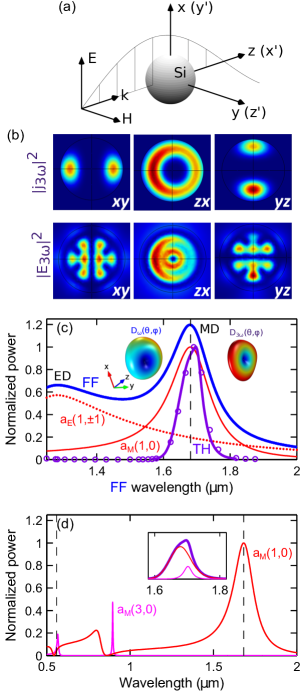
Figure 2: Third-harmonic generation by a spherical Si nanoparticle. (a) Sketch of the geometry. (b) Spatial distributions of the nonlinear current (top) and the intensity of the TH generated field (bottom) at the MD resonance, computed with FEM solver COMSOL for a dielectric particle of radius $a=230$ nm and refractive index $n=3.5$. (c) Total scattered FF (blue) and radiated TH (purple) powers spectra. Numerical results for THG are displayed with purple circle markers. Red solid and red dotted lines refer to the MD and ED contributions to the FF scattering, respectively. Insets: FF and TH radiation patterns at the MD resonance. (d) Magnetic dipole (red) and magnetic octupole (pink) contibutions to the linear scattering. Inset shows the theoretically obtained magnetic dipole (purple) and magnetic octupole (pink) relative contributions to the TH signal. Powers are normalized to the magnetic dipole maximum values.

The analytically retrieved resonant curve of the TH spectrum depicted in Fig. 2(c) was found to be consistent with the results of numerical calculations performed with the help of the finite-element method (FEM) solver COMSOL Multiphysics (see the METHODS section for details) for the particle of $n=3.5$. In our simulations, the homogeneous host medium was described by the relative dielectric permittivity $\varepsilon_{1r}=1$. Numerically calculated at the MD resonance nonlinear source and TH generated field distributions are demonstrated in Fig. 2(b). Naturally, the depicted nonlinear current, being essentially the cubed field of the MD mode excited by the pump wave, possesses a notable magnetic dipole moment. As seen in Fig. 2(c), close to the MD resonance results obtained for THG with the use of COMSOL still fit well into our analytical model that may be regarded as a shortcut of the more involved treatment exploiting the Green’s function formalism Biris and Panoiu (2010). From the above analysis, we expect only two multipoles to dominate others in the nonlinear response and visualize the spectral disposition of the generated modes around the tripled frequency. In Fig. 2(d) we plot contributions from the MD $a_{M}(1,0)$, $\propto 3|a_{M}(1,0)|^{2}/k_{0}^{2}$, and MO $a_{M}(3,0)$, $\propto 7|a_{M}(3,0)|^{2}/k_{0}^{2}$, into the linear scattering over the wide range of wavelengths, based on the exact Mie solution. Within the broad MD resonance, both magnetic dipole and magnetic octupole contribute to the THG peak, as shown in the inset of Fig. 2(d). This explains the six-petalled TH near-field structure in Fig. 2(a).

Although in this paper we do not focus specifically on the ED fundamental resonance, it is remarkable that the efficiency of THG at the MD resonance significantly exceeds that at the ED resonance. For a spherical particle, this can be shown analytically, applying the approach sketched above for the MD resonance to the case of the resonant excitation of ED. Still another formal way to quantify this effect is based on the Lorentz reciprocity theorem. Particularly, this method allows one to express the excitation coefficients of spherical multipoles, the radiated field is decomposed into, through the overlap integrals of the nonlinear source and the respective spherical modes. As discussed e.g. in Ref. O’Brien et al. (2015), such treatment, relating in essence the local-field features and far-field properties, brings in considerable intuition for the optimization of nanostructures to realize strong nonlinear response (emphasizing two key ingredients – the local field enhancement and modal overlaps). Both the approaches (to be presented in detail elsewhere) give an estimate of more than $50$ time difference between the TH radiated powers at the MD and ED resonances for the parameters of Fig. 2 and Fig. S1 of Supporting Information. Being also confirmed by the direct full-vector numerical simulations in COMSOL, this striking distinction stems from dissimilarity in spatial distribution of the respective nonlinear sources and quasipotential character of the nonlinear current induced near the ED resonance. Besides, due to the inherent curl of the source polarization induced, magnetic-type resonances in nanostructures will inevitably cause generation of magnetic multipoles, whose relative contribution into nonlinear response is usually overshadowed by more pronounced nonlinear dipole and quadrupole in metallic setups.

Generally, mirror symmetries of a scatter with respect to the planes $x=0$ and $y=0$ impose constraints on phases of the dominant excited multipolar moments. In this way, illumination by the $x$-polarized plane wave implies $a_{E}(l,-m)=-a_{E}(l,m),\>a_{M}(l,-m)=a_{M}(l,m),\>\text{if}\>m\>\text{is odd}$, and $a_{E}(l,m)=a_{M}(l,m)=0$, if $m$ is even, for the FF multipoles of the scattered field defined in the $xyz$ coordinate system. In the $x^{\prime}y^{\prime}z^{\prime}$ coordinate system we use, the aforementioned conditions formally take a more cumbersome form: $a_{E}(l,-m)=a_{E}(l,m)$, $a_{M}(l,-m)=a_{M}(l,m)$ for odd $l$, and $a_{E}(l,-m)=-a_{E}(l,m)$, $a_{M}(l,-m)=-a_{M}(l,m)$ for even $l$, where nonzero electric and magnetic multipole coefficients respond to odd or even sum of quantum numbers $(l+m)$, respectively, additionally $a_{E}(l,0)=0$. Then these relations are also expected to be fulfilled for the TH multipoles of the generated radiation if the bulk nonlinearity is isotropic. For instance in Fig. 2(c), mapping the multipole decomposition in the vector spherical harmonics basis onto the Cartesian multipole moments reflects that the coefficients $a_{E}(1,1)=a_{E}(1,-1)$ are combined to form an $x$-oriented electric dipole excitation, and $a_{M}(1,0)$ stands for the $y$-aligned magnetic dipole, with the power contributions to the linear scattering proportional to $\propto 3(|a_{E}(1,1)|^{2}+|a_{E}(1,-1)|^{2})/k_{0}^{2}$ and $\propto 3|a_{M}(1,0)|^{2}/k_{0}^{2}$, respectively.

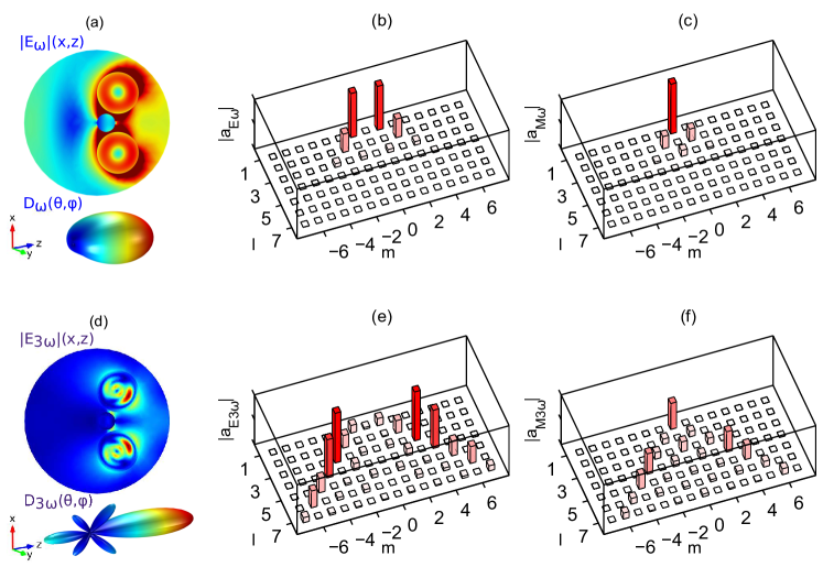
Figure 3: Control of linear and nonlinear response with a nanoparticle trimer. (a,d) Electric field distributions as seen in the $xz$ plane, 3D far-field radiation patterns and magnitudes of the electric (b,e) and (c,f) magnetic multipole moments of the fields at FF (top row) and TH (bottom row) calculated for a trimer of dielectric spheres aligned on their left and excited by the $x$-polarized plane wave incident from the left with the wavelength $1.68$ $\mu$m corresponding to the fundamental MD resonance of a single large sphere. The radii of the larger spheres and small sphere are $230$ nm and $100$ nm, respectively. Center-to-center distances between the particles are $660$ nm and $355$ nm, refractive index of the particles $n=3.5$.

Note that within our model we assumed the cubic volume nonlinearity of a dielectric scatterer isotropic and characterized by a scalar third-order susceptibility, which is true for amorphous silicon (a-Si). Actual material dispersion and dissipative losses in a-Si, that can be extracted experimentally from ellipsometric measurements, may become nonnegligible at TH frequency and will affect the TH emission spectra. For the parameters of Fig. 2, these dispersive factors only slightly deviate the linear scattering properties at FF, while at TH they influence mainly the region near the ED resonance, where the conversion efficiency is much lower than that near MD resonance. However, depending on the optical properties of the sample, they may cause a spectral separation of the MD and MO contributions in the nonlinear scattering (similar to that shown in Fig. 1S of Supporting Information) and and transformations of TH radiation patterns due to alterations in phases of the generated field multipoles, decreasing the total radiated power by a factor of $40$ at the incident intensity $1$ GW/cm², as it follows from the numerical simulations rectified with the wavelength-dependent complex-value refractive index of a-Si.

Control over third-harmonic directionality

For a single spherical particle, we found the radiation pattern of the most efficient THG at the magnetic dipole resonance to be predominantly axially symmetric that does not allow for the emission directionality. Apparently, it also holds for a dimer of spheres under the longitudinal illumination (when the electric field of the incident plane wave is directed along the dimer axis). To shape the TH radiation pattern, one can play with geometry. For instance, placing a small particle near the dimer drastically modifies both the linear and nonlinear response due to inter-particle interaction, as exemplified in Fig. 3. The fundamental frequency of the impinging wave is chosen to match the MD resonance of an individual large sphere. The small particle, acting as an electric dipole at this wavelength when isolated, is magnificantly excited by the resonant co-circulating electric near-fields of the larger neighbors. As a result, the linear scattering contains both electric and magnetic dipoles and forward-directed, while the TH emission acquires directivity due to the excitation of higher-order multipoles, with six lobes indicating the leading electric octupole $a_{E}(3,\pm 3)$.

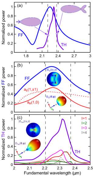
Figure 4: Resonant nonlinear directional scattering from a Si nanodisk. (a) Numerical spectra of the total FF scattered (blue line) and TH radiated (purple line) powers calculated for a single disk with radius $r_{d}=390$ nm, thickness $h=390$ nm, and refractive index $n=3.5$ suspended in air. Callouts depict the forward- and backward-directed far-field radiation patterns on the different sides of the TH peak, as indicated by points and thin vertical dashed lines. (b) Linear scattering spectrum (blue solid curve) overlaid with MD (red solid) and ED (red dotted) contributions to the scattering. (c) Total TH radiated power (solid purple line) decomposed into multipolar contributions of different orbital numbers $l$. The color solid and dotted curves refer to the main magnetic and electric contributions to the radiation, respectively. Insets in panels (b) and (c) show 3D radiation patterns and the electric field magnitude distributions in the $xz$ plane at FF and TH at the spectral point corresponding to the forward-directed TH emission, illustrated in Fig. 1. Powers are normalized to the magnetic dipole maximum values.

Alternatively, magnetic and electric dipolar eigenmodes can be spectrally overlapped using only one structural element, such as ellipsoid or cylinder, by adjusting aspect-ratio. We calculate numerically the nonlinear response of the disk, presumably made of crystalline Si (c-Si), with the radius and height equal to each other, $r_{d}=h=390$ nm. Geometrical parameters of the disk are chosen to escape dramatic influence of dispersion and losses at both fundamental and TH frequencies, and we approximately set the refractive index constant $n=3.5$ in our simulations. In c-Si the nonlinear polarization at the third-harmonic frequency is given by Moss et al. (1989) $P^{(3)}_{i}=\varepsilon_{0}\left\{3\chi^{(3)}_{1122}E_{i}({\bf E}\cdot{\bf E})+\left[\chi^{(3)}_{1111}-3\chi^{(3)}_{1122}\right]E_{i}^{3}\right\}$, with the second term responsible for anisotropy which is a complex-valued frequency-dependent function in general case. However, for low enough photon energies $\hbar\omega\lesssim 0.6$ eV ($\lambda\gtrsim 2$ $\mu$m), it was established that two components of the third-order susceptibility are related as $\chi^{(3)}_{1111}=2.36\chi^{(3)}_{1122}$ Vivien and Pavesi (2013). In fact, this anisotropy in the wavelength window considered was not found to result in very substantial alterations in THG, as compared to the case when the isotropic cubic susceptibility is attributed to the nonlinear disk-shaped scatterer. The results obtained are summarized in Fig. 4.

In the nonlinear response, on calculating multipole decomposition, we observe strong excitation of the following multipole moments up to $l=4$: $a_{E}(1,\pm 1)$, $a_{M}(1,0)$, $a_{E}(2,\pm 2)$, $a_{M}(2,\pm 1)$, $a_{E}(3,\pm 3)$, $a_{M}(3,\pm 2)$, $a_{M}(3,\pm 0)$, $a_{E}(4,\pm 4)$, $a_{E}(4,\pm 2)$, $a_{M}(4,\pm 3)$, $a_{M}(4,\pm 1)$. Their amplitudes are sharply frequency-dependent. All others give negligible contributions. Near the intersection point of red dotted and red solid lines in Fig. 4(b) [where the strengths of the excited electric and magnetic dipoles are matched (i.e. $p_{x}\approx\sqrt{\varepsilon_{0}\mu_{0}}m_{y}$), thus producing directional scattering], interference between the nonlinear multipoles of opposite parities gives rise to an unidirectional lobe at TH. On the opposite slope of the TH peak, the lobe switches its direction.

To quantify the efficiency of nonlinear conversion, we define the THG efficiency for a single disk ${\eta}^{\text{THG}}$ as the ratio of the total TH radiated power to the energy flux of the fundamental wave through the physical area of the disk, ${\eta}^{\text{THG}}=\displaystyle\frac{W_{s}^{\text{TH}}}{I_{0}\pi r_{d}^{2}}$, where $I_{0}=\displaystyle\frac{|E_{0}|^{2}}{2\eta}$ is the incident field intensity. Near the resonance, the disk exhibits ${\eta}^{\text{THG}}\sim 10^{-5}$ at $I_{0}=1$ GW/cm² and the value of the nonlinear susceptibility in this frequency range estimated as $3\chi^{(3)}_{1122}\approx 2.2\times 10^{-19}$ (m/V)², based on the data in Ref. Moss et al. (1990).

Importantly, the efficiency of nonlinear optical processes in Si is known to be limited by two-photon absorption (TPA) Lin et al. (2007); Shcherbakov et al. (2015b). At high intensities of light, TPA and subsequent free-carrier absorption (FCA) introduce considerable undesired optical loss and change the refractive index. Generally, TPA is strong in near-infrared, being essentially wavelength-dependent and anisotropic, but drops significantly with increasing the operating wavelength and vanishes at 2.2 $\mu$m. The parameters of Fig. 4 match the range with reduced TPA. However, depending on the operating conditions, the model described in this paper should be extended to account for the relevant effects. In particular, the dependence of the refractive index on the incident field intensity, the so-called self-action associated with Kerr effect and TPA, may shift and broaden Mie resonances and thereby affect THG, raising the need for a more-involved self-consistent model analogous to that developed in Ref. Ginzburg et al. (2015) for harmonic generation in metallic nanostructures. Nonetheless, for the parameters of Fig. 4, at the incident energy flux density of $\sim 1$ GW/cm² the influence of the Kerr effect and TPA on THG can be neglected, since the nonlinear shift of the resonance $\Delta\lambda_{0}^{\text{(NL)}}$ far exceeds its nonlinear broadening and three orders of magnitude smaller than the width of the Mie resonance (using the data from Ref. Lin et al. (2007), the estimate gives $\Delta\lambda_{0}^{\text{(NL)}}/\lambda_{0}\sim\Delta n^{\text{(NL)}}/n\sim 10^{-4}$, where $\Delta n^{\text{(NL)}}$ is a nonlinear correction to the refractive index).

CONCLUSION

We have discussed the third-harmonic generation in all-dielectric resonant nanostructures exhibiting optically-induced Mie-type magnetic response and have demonstrated that such structures offer important tools for tailoring the efficiency and directionality of nonlinear emission at the nanoscale, in particular, by employing the properties of higher-order magnetic multipole moments of the generated field. This framework suggests many novel opportunities for a design of nonlinear subwavelength light sources with reconfigurable radiation characteristics and engineering magnetic optical nonlinearities in nanostructured dielectric metadevices.

METHODS

Multipole decomposition. We adopt the following well-established standard form of the multipole expansion for the scattered (or radiated) field written in the spherical coordinates Jackson (1965); Grahn et al. (2012) (accepting harmonic time-dependence $\sim e^{-i\omega t}$):

$${\bf E}_{s}\left({\omega;r,\theta,\varphi}\right)=E_{0}\sum_{l=1}^{\infty}\sum_{m=-l}^{l}i^{l}\sqrt{\pi(2l+1)}\Big{\{}a_{{M}}(l,m)h_{l}^{(1)}(kr){\bf X}_{lm}(\theta,\varphi)$$

$$+\frac{1}{k}a_{{E}}(l,m)\nabla\times\big{[}h_{l}^{(1)}(kr){\bf X}_{lm}(\theta,\varphi)\big{]}\Big{\}},$$ (15)

$${\bf H}_{{s}}\left({\omega;r,\theta,\varphi}\right)=\frac{E_{0}}{\eta}\sum_{l=1}^{\infty}\sum_{m=-l}^{l}i^{l-1}\sqrt{\pi(2l+1)}\Big{\{}a_{{E}}(l,m)h_{l}^{(1)}(kr){\bf X}_{lm}(\theta,\varphi)$$

$$+\frac{1}{k}a_{{M}}(l,m)\nabla\times\big{[}h_{l}^{(1)}(kr){\bf X}_{lm}(\theta,\varphi)\big{]}\Big{\}},$$ (16)

where ${\bf{X}}_{l,m}=\displaystyle\frac{-1}{\sqrt{l(l+1)}}\biggl{\{}0,\displaystyle\frac{mY_{l,m}(\theta,\varphi)}{\sin{\theta}},i\displaystyle\frac{\partial Y_{l,m}(\theta,\varphi)}{\partial\theta}\biggr{\}}$ are the vector spherical harmonics expressed through the scalar spherical harmonics $Y_{l,m}(\theta,\varphi)$, $h_{l}^{(1)}$ are the spherical Hankel functions of the first kind with the asymptotics of outgoing spherical waves, $k=\omega\sqrt{\varepsilon\mu}\equiv k_{0}\sqrt{\varepsilon_{r}\mu_{r}}$ is the wavenumber in the medium, $\eta=\sqrt{\mu/\varepsilon}$ is the impedance, $E_{0}$ is an electric field amplitude factor. The electric $a_{{E}}(l,m)$ and magnetic $a_{{M}}(l,m)$ multipole cofficients can be found either through the volume integration of the source current density distribution, or by using angular integrals of radial components of the numerically pre-calculated scattered field over a spherical surface of some radius $r$ enclosing an isolated scatterer as follows:

$$a_{{E}}(l,m) =\displaystyle\frac{(-i)^{l+1}kr}{h_{l}^{(1)}(kr)E_{0}\sqrt{\pi(2l+1)l(l+1)}}\displaystyle{\int_{0}^{2\pi}\int_{0}^{\pi}Y^{*}_{lm}(\theta,\varphi)\hat{{\bf r}}\cdot{\bf E}_{{s}}({\bf r})\sin\theta d\theta d\varphi},$$ (17a)

$$a_{{M}}(l,m) =\displaystyle\frac{(-i)^{l}\eta kr}{h_{l}^{(1)}(kr)E_{0}\sqrt{\pi(2l+1)l(l+1)}}\displaystyle{\int_{0}^{2\pi}\int_{0}^{\pi}Y^{*}_{lm}(\theta,\varphi)\hat{{\bf r}}\cdot{\bf H}_{{s}}({\bf r})\sin\theta d\theta d\varphi}.$$ (17b)

In terms of these scattering coefficients, the total time-averaged scattered power (energy flow) is given as

$$W_{s}=\displaystyle\frac{\pi|E_{0}|^{2}}{2\eta k^{2}}\sum\limits_{l=1}^{\infty}\sum\limits_{m=-l}^{l}{(2l+1)\left(|a_{E}(l,m)|^{2}+|a_{M}(l,m)|^{2}\right)},$$ (18)

revealing the input of each multipolar excitation.

Numerical simulation method. The nonlinear response of nanostructures is simulated in FEM solver COMSOL Multiphysics using two coupled electromagnetic models Smirnova et al. (2015), assuming the undepleted pump field. First, we simulate the linear scattering through the excitation of the nanostructure with a plane wave and compute the nonlinear polarization induced in the bulk of the nanostructure. Second, this polarization is employed as a source for the next electromagnetic simulation at the TH frequency, and the generated field is recovered. This method can be applied to nanostructures of complex three-dimensional geometries, and it can be straightforwardly extended to account for the surface nonlinear response.

Supporting Information

Single-mode approximation

The analytical theory developed in the paper describes the third-harmonic generation (THG) from a high-permittivity dielectric sphere under the resonant excitation by a plane wave, assuming the nonlinear conversion process is predominantly governed by the corresponding resonant multipolar mode. Generally speaking, such approximation is valid only if the refractive index of the dielectric is sufficiently large and multipolar resonances do not overlap strongly. We illustrate this case for the refractive index $n=6$ in Fig. S1. The value of $n$, unpractical in the infrared and optical frequency ranges, is considered here merely for methodological clarity and also for the verification of our analytical formulas. All calculations in the main text are performed with the focus on silicon, which is one of the primary materials employed in nonlinear dielectric nanophotonics.

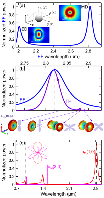
Figure 5: Third-harmonic generation by a spherical high-index nanoparticle near the magnetic resonance. (a) Power spectrum of linear scattering calculated for a lossless high-index spherical dielectric particle of radius $a=230$ nm and refractive index $n=6$, excited by the $x$-polarized plane wave. Insets: sketch of the geometry; the electric field norm distribution in the $xz$ plane at the electric and magnetic dipole resonances. (b) Scattered FF power (blue line) and radiated TH power (purple line) in the vicinity of the MD resonance as functions of the fundamental wavelength. Callouts illustrate TH radiation patterns and their cross-sections in the $xy$ plane at $4$ spectral points. (c) Magnetic dipole (red) and magnetic octupole (pink) contibutions to the linear scattering. Inset: cross-sections of radiation patterns for the magnetic dipole (red) and magnetic octupole (pink) in the $xy$ plane. Positions of the MD resonant wavelength and the respective TH wavelength are marked by vertical dashed black lines. Powers are normalized to the magnetic dipole maximum values.

If the refractive index is high enough, electric (ED) and magnetic (MD) dipolar resonances are well-separated in frequency and rather narrow, as shown in Fig. S1(a). The analytically calculated TH power dependence, perfectly matching the numerical results obtained with the use of the finite-element method solver COMSOL Multiphysics, is plotted in Fig. S1(b) as a function of the wavelength of the incident radiation, where we also demonstrate variations of the TH emission pattern, originating from the interference of the magnetic dipole and magnetic octupole, though preserving azimuthal (with respect to the $y$ axis) symmetry. To elucidate a slight blue-shift of the THG peak from the fundamental MD wavelength, as well as appearance of the side small peak observed, in Fig. S1(c) we plot contributions from the magnetic dipole $a_{M}(1,0)$, $\propto 3|a_{M}(1,0)|^{2}/k_{0}^{2}$, and magnetic octupole $a_{M}(3,0)$, $\propto 7|a_{M}(3,0)|^{2}/k_{0}^{2}$, into the linear scattering over the wide range of wavelengths, based on the exact Mie solution. Each multipole has an infinite number of resonances. From our analysis, we expect only two multipoles to dominate others in the nonlinear response and visualize the spectral disposition of the generated modes around the tripled frequency. The small side peak is seen to be associated with the octupole resonance near the tripled frequency.

Despite the single mode approximation made in the derivation of the analytical theory, we notice that its applicability successively holds for the lower value of refractive index $n=3.5$ corresponding to silicon. The results of analytical and first-principles calculations in the proximity of the magnetic dipole resonance agree extremely well in both the cases $n=6$ and $n=3.5$ (the latter is presented in Fig. 2 of the main text). However, the magnetic dipolar and octupolar contributions to the nonlinear scattering are hidden under a common THG peak associated with the fundamental MD resonance for $n=3.5$, being clearly separated in frequency for $n=6$.

References

- Jahani and Jacob (2016) S. Jahani and Z. Jacob, Nat. Nanotechnol. 11, 23 (2016).
- Garcia-Etxarri et al. (2011) A. Garcia-Etxarri, R. Gómez-Medina, L. S. Froufe-Pérez, C. López, L. Chantada, F. Scheffold, J. Aizpurua, M. Nieto-Vesperinas, and J. J. Sáenz, Opt. Express 19, 4815 (2011).
- Schmidt et al. (2012) M. K. Schmidt, R. Esteban, J. J. Sáenz, I. Suárez-Lacalle, S. Mackowski, and J. Aizpurua, Opt. Express 20, 13636 (2012).
- Evlyukhin et al. (2012) A. B. Evlyukhin, S. M. Novikov, U. Zywietz, R. L. Eriksen, C. Reinhardt, S. I. Bozhevolnyi, and B. N. Chichkov, Nano Lett. 12, 3749 (2012).
- Kuznetsov et al. (2012) A. I. Kuznetsov, A. E. Miroshnichenko, Y. H. Fu, J. Zhang, and B. Luk’yanchuk, Sci. Rep. 2, 492 (2012).
- Staude et al. (2013) I. Staude, A. E. Miroshnichenko, M. Decker, N. T. Fofang, S. Liu, E. Gonzales, J. Dominguez, T. S. Luk, D. N. Neshev, I. Brener, and Y. Kivshar, ACS Nano 7, 7824 (2013).
- Zywietz et al. (2014) U. Zywietz, A. B. Evlyukhin, C. Reinhardt, and B. N. Chichkov, Nat. Commun. 5, 4402 (2014).
- Liu et al. (2014a) S. Liu, M. B. Sinclair, T. S. Mahony, Y. C. Jun, S. Campione, J. Ginn, D. A. Bender, J. R. Wendt, J. F. Ihlefeld, P. G. Clem, J. B. Wright, and I. Brener, Optica 1, 250 (2014a).
- Zywietz et al. (2015) U. Zywietz, M. K. Schmidt, A. B. Evlyukhin, C. Reinhardt, J. Aizpurua, and B. N. Chichkov, ACS Photonics 2, 913 (2015).
- Palik (1985) E. D. Palik, ed., Handbook of Optical Constants of Solids (Academic, Orlando, 1985).
- Burns and Bloembergen (1971) W. K. Burns and N. Bloembergen, Phys. Rev. B 4, 3437 (1971).
- Moss et al. (1989) D. J. Moss, H. M. van Driel, and J. E. Sipe, Opt. Lett. 14, 57 (1989).
- Moss et al. (1990) D. J. Moss, E. Ghahramani, J. E. Sipe, and H. M. van Driel, Phys. Rev. B 41, 1542 (1990).
- Bristow et al. (2007) A. D. Bristow, N. Rotenberg, and H. M. van Driel, Appl. Phys. Lett. 90, 191104 (2007).
- Lin et al. (2007) Q. Lin, J. Zhang, G. Piredda, R. W. Boyd, P. M. Fauchet, and G. P. Agrawal, Appl. Phys. Lett. 91, 021111 (2007).
- Zhang et al. (2007) J. Zhang, Q. Lin, G. Piredda, R. W. Boyd, G. P. Agrawal, and P. M. Fauchet, Appl. Phys. Lett. 91, 071113 (2007).
- Ikeda et al. (2007) K. Ikeda, Y. Shen, and Y. Fainman, Opt. Express 15, 17761 (2007).
- Vivien and Pavesi (2013) L. Vivien and L. Pavesi, eds., Handbook of Silicon Photonics (Taylor & Francis, 2013).
- Gai et al. (2014) X. Gai, D.-Y. Choi, and B. Luther-Davies, Opt. Express 22, 9948 (2014).
- Shcherbakov et al. (2014) M. R. Shcherbakov, D. N. Neshev, B. Hopkins, A. S. Shorokhov, I. Staude, E. V. Melik-Gaykazyan, M. Decker, A. A. Ezhov, A. E. Miroshnichenko, I. Brener, A. A. Fedyanin, and Y. S. Kivshar, Nano Lett. 14, 6488 (2014).
- Shcherbakov et al. (2015a) M. R. Shcherbakov, A. S. Shorokhov, D. N. Neshev, B. Hopkins, I. Staude, E. V. Melik-Gaykazyan, A. A. Ezhov, A. E. Miroshnichenko, I. Brener, A. A. Fedyanin, and Y. S. Kivshar, ACS Photonics 2, 578 (2015a).
- Shcherbakov et al. (2015b) M. R. Shcherbakov, P. P. Vabishchevich, A. S. Shorokhov, K. E. Chong, D.-Y. Choi, I. Staude, A. E. Miroshnichenko, D. N. Neshev, A. A. Fedyanin, and Y. S. Kivshar, Nano Lett. 15, 6985 (2015b).
- Jackson (1965) J. Jackson, Classical electrodynamics (Mir, Moskow, 1965).
- Bohren and Huffman (1983) C. F. Bohren and D. R. Huffman, Absorption and Scattering of Light by Small Particles (Wiley, New York, 1983).
- Dadap et al. (1999) J. I. Dadap, J. Shan, K. B. Eisenthal, and T. F. Heinz, Phys. Rev. Lett. 83, 4045 (1999).
- Dadap et al. (2004) J. I. Dadap, J. Shan, and T. F. Heinz, J. Opt. Soc. Am. B 21, 1328 (2004).
- Kujala et al. (2008) S. Kujala, B. K. Canfield, M. Kauranen, Y. Svirko, and J. Turunen, Opt. Express 16, 17196 (2008).
- Petschulat et al. (2009) J. Petschulat, A. Chipouline, A. Tünnermann, T. Pertsch, C. Menzel, C. Rockstuhl, and F. Lederer, Phys. Rev. A 80, 063828 (2009).
- Gonella and Dai (2011) G. Gonella and H.-L. Dai, Phys. Rev. B 84, 121402 (2011).
- Mühlig et al. (2011) S. Mühlig, C. Menzel, C. Rockstuhl, and F. Lederer, Metamaterials 5, 64 (2011).
- Huttunen et al. (2012) M. J. Huttunen, J. Mäkitalo, G. Bautista, and M. Kauranen, New J. Phys. 14, 113005 (2012).
- Capretti et al. (2012) A. Capretti, G. F. Walsh, S. Minissale, J. Trevino, C. Forestiere, G. Miano, and L. D. Negro, Opt. Express 20, 15797 (2012).
- Grahn et al. (2012) P. Grahn, A. Shevchenko, and M. Kaivola, New J. Phys. 14, 093033 (2012).
- Liu et al. (2012) W. Liu, A. E. Miroshnichenko, D. N. Neshev, and Y. S. Kivshar, ACS Nano 6, 5489 (2012).
- Rodrigo et al. (2013) S. G. Rodrigo, H. Harutyunyan, and L. Novotny, Phys. Rev. Lett. 110, 177405 (2013).
- Fu et al. (2013) Y. H. Fu, A. I. Kuznetsov, A. E. Miroshnichenko, Y. F. Yu, and B. Luk’yanchuk, Nat. Commun. 4, 1527 (2013).
- Poutrina et al. (2013) E. Poutrina, A. Rose, D. Brown, A. Urbas, and D. R. Smith, Opt. Express 21, 31138 (2013).
- Krasnok et al. (2014a) A. E. Krasnok, C. R. Simovski, P. A. Belov, and Y. S. Kivshar, Nanoscale 6, 7354 (2014a).
- Smirnova et al. (2014) D. A. Smirnova, I. V. Shadrivov, A. E. Miroshnichenko, A. I. Smirnov, and Y. S. Kivshar, Phys. Rev. B 90, 035412 (2014).
- Davidson II et al. (2015) R. B. Davidson II, J. I. Ziegler, G. Vargas, S. M. Avanesyan, Y. Gong, W. Hess, and R. F. Haglund Jr., Nanophotonics 4, 2 (2015).
- Dregely et al. (2014) D. Dregely, K. Lindfors, M. Lippitz, N. Engheta, M. Totzeck, and H. Giessen, Nat. Commun. 5, 5354 (2014).
- Liberal et al. (2015) I. Liberal, I. Ederra, R. Gonzalo, and R. W. Ziolkowski, J. Opt. 17, 072001 (2015).
- Kerker et al. (1983) M. Kerker, D.-S. Wang, and C. L. Giles, J. Opt. Soc. Am. B 73, 765 (1983).
- Liu et al. (2014b) W. Liu, J. Zhang, B. Lei, H. Ma, W. Xie, and H. Hu, Opt. Express 22, 16178 (2014b).
- Hancu et al. (2014) I. M. Hancu, A. G. Curto, M. Castro-López, M. Kuttge, and N. F. van Hulst, Nano Lett. 14, 166 (2014).
- Naraghi et al. (2015) R. R. Naraghi, S. Sukhov, and A. Dogariu, Opt. Lett. 40, 585 (2015).
- Alaee et al. (2015) R. Alaee, R. Filter, D. Lehr, F. Lederer, and C. Rockstuhl, Opt. Lett. 40, 2645 (2015).
- Kauranen and Zayats (2012) M. Kauranen and A. V. Zayats, Nat. Photonics 6, 737 (2012).
- Boyd (2008) R. W. Boyd, Nonlinear Optics, 3rd ed. (Elsevier, New York, 2008).
- Hayat and Orenstein (2007) A. Hayat and M. Orenstein, Opt. Lett. 32, 2864 (2007).
- Banaee and Crozier (2011) M. G. Banaee and K. B. Crozier, ACS Nano 5, 307 (2011).
- Thyagarajan et al. (2012) K. Thyagarajan, S. Rivier, A. Lovera, and O. J. Martin, Opt. Express 20, 12860 (2012).
- Navarro-Cia and Maier (2012) M. Navarro-Cia and S. A. Maier, ACS Nano 6, 3537 (2012).
- Aouani et al. (2012) H. Aouani, M. Navarro-Cia, M. Rahmani, T. P. H. Sidiropoulos, M. Hong, R. F. Oulton, and S. A. Maier, Nano Letters 12, 4997 (2012).
- Ginzburg et al. (2012) P. Ginzburg, A. Krasavin, Y. Sonnefraud, A. Murphy, R. J. Pollard, S. A. Maier, and A. V. Zayats, Phys. Rev. B 86, 085422 (2012).
- Roke and Gonella (2012) S. Roke and G. Gonella, Annu. Rev. Phys. Chem. 63, 353 (2012).
- Butet et al. (2015) J. Butet, P.-F. Brevet, and O. J. F. Martin, ACS Nano 9, 10545 (2015).
- Segovia et al. (2015) P. Segovia, G. Marino, A. V. Krasavin, N. Olivier, G. A. Wurtz, P. A. Belov, P. Ginzburg, and A. V. Zayats, Opt. Express 23, 30730 (2015).
- Metzger et al. (2012) B. Metzger, M. Hentschel, M. Lippitz, and H. Giessen, Opt. Lett. 37, 4741 (2012).
- Hentschel et al. (2012) M. Hentschel, T. Utikal, H. Giessen, and M. Lippitz, Nano Lett. 12, 3778 (2012).
- Metzger et al. (2014) B. Metzger, T. Schumacher, M. Hentschel, M. Lippitz, and H. Giessen, ACS Photonics 1, 471 (2014).
- Zhang et al. (2013) Y. Zhang, F. Wen, Y.-R. Zhen, P. Nordlander, and N. J. Halas, Proc. Natl. Acad. Sci. USA 110, 9215 (2013).
- Dewitz et al. (1996) J. Dewitz, W. Hübner, and K. Bennemann, Z. Phys. D 37, 75 (1996).
- Pavlyukh and Hübner (2004) Y. Pavlyukh and W. Hübner, Phys. Rev. B 70, 245434 (2004).
- de Beer and Roke (2009) A. G. F. de Beer and S. Roke, Phys. Rev. B 79, 155420 (2009).
- Butet et al. (2012) J. Butet, I. Russier-Antoine, C. Jonin, N. Lascoux, E. Benichou, and P.-F. Brevet, J. Opt. Soc. Am. B 29, 2213 (2012).
- Bachelier et al. (2010) G. Bachelier, J. Butet, I. Russier-Antoine, C. Jonin, E. Benichou, and P.-F. Brevet, Phys. Rev. B 82, 235403 (2010).
- Wang et al. (2009) F. X. Wang, F. J. Rodríguez, W. M. Albers, R. Ahorinta, J. E. Sipe, and M. Kauranen, Phys. Rev. B 80, 233402 (2009).
- Shadrivov et al. (2015) I. V. Shadrivov, M. Lapine, and Y. S. Kivshar, eds., Nonlinear, Tunable and Active Metamaterials (Springer International Publishing, 2015).
- Rose et al. (2013) A. Rose, D. Huang, and D. R. Smith, Phys. Rev. Lett. 110, 063901 (2013).
- Kruk et al. (2015) S. Kruk, M. Weismann, A. Y. Bykov, E. A. Mamonov, I. A. Kolmychek, T. Murzina, N. C. Panoiu, D. N. Neshev, and Y. S. Kivshar, ACS Photonics 2, 1007 (2015).
- Bharadwaj et al. (2009) P. Bharadwaj, B. Deutsch, and L. Novotny, Adv. Opt. Photon. 1, 438 (2009).
- Novotny and van Hulst (2011) L. Novotny and N. van Hulst, Nat. Photonics 5, 83 (2011).
- Krasnok et al. (2013) A. E. Krasnok, I. S. Maksymov, A. I. Denisyuk, P. A. Belov, A. E. Miroshnichenko, C. R. Simovski, and Y. S. Kivshar, Physics-Uspekhi 56, 539 (2013).
- Krasnok et al. (2014b) A. E. Krasnok, P. A. Belov, A. E. Miroshnichenko, A. I. Kuznetsov, B. S. Lukyanchuk, and Y. S. Kivshar, in Progress in Compact Antennas (InTech, 2014).
- Biris and Panoiu (2010) C. G. Biris and N. C. Panoiu, Phys. Rev. B 81, 195102 (2010).
- O’Brien et al. (2015) K. O’Brien, H. Suchowski, J. Rho, A. Salandrino, B. Kante, X. Yin, and X. Zhang, Nat. Mater. 14, 379 (2015).
- Ginzburg et al. (2015) P. Ginzburg, A. V. Krasavin, G. A. Wurtz, and A. V. Zayats, ACS Photonics 2, 8 (2015).
- Smirnova et al. (2015) D. A. Smirnova, A. E. Miroshnichenko, Y. S. Kivshar, and A. B. Khanikaev, Phys. Rev. B 92, 161406 (2015).