NLO efforts in Herwig++

Abstract:

With the advent and recent extension of the BLHA standard to interface Monte Carlo event generators and one-loop matrix element providers, the Herwig++ event generator has expanded its range of applicability to a multitude of underlying hard processes at NLO QCD. The new NLO development is centered around the Matchbox framework, which turns fixed NLO QCD calculations into parton shower matched calculations - to be matched to the two parton shower variants of Herwig++. Matchbox provides thereby for the automated setup of the underlying fixed NLO QCD calculations and the interface to the one-loop matrix element providers, as well as for an efficient and automated multi-channel phase space sampling, and forms the basis for the NLO capabilities of the new release of Herwig++. Along with several other new features and developments, the new release marks the end of distinguishing Herwig++ and (Fortran) HERWIG, and constitutes the first major release of version 7 of the Herwig event generator.

HERWIG-2016-01, KA-TP-03-2016, MCnet-16-01

1 Introduction

The new release of version 7 of the Herwig event generator [1] marks the end of distinguishing Herwig++ [2, 3] and HERWIG [4] and the point at which the physics capabilities of both its predecessors (from the Herwig++ 2 series and the HERWIG 6 series) are superseded.

Herwig is a computer program for the simulation of exclusive event generation in particle collisions at hadron-hadron, hadron-lepton, and lepton-lepton colliders. It is written in the programming language C++ and based on ThePEG, which in the new version 2.0 is available for download along with Herwig 7.0 at https://herwig.hepforge.org/downloads.

Herwig features the full simulation of particle collision events up to the particle level, i.e. perturbative as well as non-perturbative physics. The perturbative part provides the simulation of hard processes at NLO QCD (including several built-in LO and NLO matrix elements, LH event file input as well as the fully automated assembly of NLO QCD calculations for almost all Standard Model processes, utilizing various interfaces to several external matrix element providers), shower Monte Carlos (facilitating two coherent shower algorithms - an angular-ordered parton shower [5] as well as a dipole shower [6], including the simulation of decays with full spin correlations), as well as the corresponding LO and NLO matching procedures (dedicated matrix element corrected shower plug-ins and built-in Powheg matched cross sections, as well as a fully automated matching machinery, with algorithms based on MC@NLO- [7] and Powheg-type [8] matching). The non-perturbative part offers the simulation of the hadronization process (utilizing the cluster hadronization model) as well as of the underlying event (utilizing an eikonal multiple interaction model). In addition, Herwig features a highly flexible machinery for BSM processes (including built-in BSM matrix elements as well as UFO model input capabilities).

2 NLO Automatization and Matching

Automated NLO matching and merging requires full control over the fixed-order input and hence the need for a fully integrated framework arises. The previoulsy developed Matchbox framework [9] provides such functionality and its extension forms the basis for the automated NLO capabilities of the new Herwig release.

Based on the Matchbox framework the new Herwig release facilitates the automated setup of all processes and ingredients necessary for a full NLO QCD calculation in the subtraction formalism: an implementation of the dipole subtraction method based on the approach by Catani and Seymour (including massive dipole subtraction) [10, 11], as well as interfaces to various external matrix element providers, or to in-house calculations for the hard sub-processes such as electroweak corrections to the production of heavy vector boson pairs [12, 13, 14] or amplitudes for electroweak Higgs plus jets production provided by the HJets++ plug-in to Matchbox. Fully automated matching algorithms are available, inspired by MC@NLO- [7] and Powheg-type [8] matching (referred to as subtractive and multiplicative matching respectively), for the systematic and consistent combination of NLO QCD calculations with both shower variants in Herwig [5, 6].

Consider the subtractive matching for example. An observable $O_{\mathrm{NLO}}$ at NLO QCD, whose leading order contribution for $n$ final state partons is given by $O_{\mathrm{LO}}=\int\mathrm{d}\Phi_{n}\mathpzc{B}O_{n}$, can in a condensed notation in the subtraction formalism be written as

$$O_{\mathrm{NLO}}=\int\mathrm{d}\Phi_{n}\Big{(}\mathpzc{B}+\bar{\mathpzc{V}}\Big{)}O_{n}+\int\mathrm{d}\Phi_{n+1}\Big{(}\mathpzc{R}O_{n+1}-\mathpzc{A}O_{n}\Big{)}\;\;,\quad\bar{\mathpzc{V}}=\mathpzc{V}+\int\mathrm{d}\Phi_{1}\mathpzc{A}$$ (1)

where $\mathpzc{B}$ denotes the corresponding Born matrix element, $\mathpzc{V}$ the UV-subtracted virtual contribution, $\mathpzc{R}$ the real contribution and $\mathpzc{A}$ the subtraction term (the contribution from the collinear counter term to subtract additional initial state collinear singularities is hereby neglected). The subtractive matching formula can correspondingly be written in a condensed notation as shown in eq. (2)

$$O^{\rm{matched}}_{\rm{NLO}}=\Bigg{[} \displaystyle\int\mathrm{d}\Phi_{n}\Big{(}\leavevmode\hbox to13.75pt{\vbox to13.5pt{\text{[drawing]}}}+\leavevmode\hbox to11.67pt{\vbox to12.34pt{\text{[drawing]}}}\Big{)}+\displaystyle\int\mathrm{d}\Phi_{n}\leavevmode\hbox to13.75pt{\vbox to13.5pt{\text{[drawing]}}}\displaystyle\int^{Q^{2}}_{\mu^{2}_{IR}}\mathrm{d}\leavevmode\hbox to24.33pt{\vbox to16.67pt{\text{[drawing]}}}-\displaystyle\int\mathrm{d}\Phi_{n+1}\leavevmode\hbox to14.17pt{\vbox to13.5pt{\text{[drawing]}}}\Theta(q^{2}-\mu^{2}_{IR})\Bigg{]}O_{n} \mathpzc{B} \bar{\mathpzc{V}} \mathpzc{B} \!\!\!\mathpzc{P}(q^{2}) \mathpzc{A}$$

$$+\Bigg{[} \displaystyle\int\mathrm{d}\Phi_{n+1}\leavevmode\hbox to14.03pt{\vbox to13.5pt{\text{[drawing]}}}-\displaystyle\int\mathrm{d}\Phi_{n}\leavevmode\hbox to13.75pt{\vbox to13.5pt{\text{[drawing]}}}\displaystyle\int^{Q^{2}}_{\mu^{2}_{IR}}\mathrm{d}\leavevmode\hbox to25.88pt{\vbox to18.67pt{\text{[drawing]}}}-\displaystyle\int\mathrm{d}\Phi_{n+1}\leavevmode\hbox to14.17pt{\vbox to13.5pt{\text{[drawing]}}}\Theta\big{(}\mu^{2}_{IR}-q^{2}\big{)}\Bigg{]}O_{n+1} \mathpzc{R} \mathpzc{B} \!\!\!\mathpzc{P}\big{(}q^{2}\big{)} \mathpzc{A}$$ (2)

where $\mathpzc{P}(q^{2})$ denotes the shower kernel, evaluated at the shower evolution scale $q$, $Q$ the hard process scale (aka the shower start scale) and $\mu_{\mathrm{IR}}$ the shower cut-off scale, and which is rearranged with respect to $O_{n}$ and $O_{n+1}$, i.e. in terms of so-called $S$- and $H$-events respectively.

For the Born, virtual, real and subtraction term contributions various interfaces to matrix element code exist: either at the level of squared matrix elements through the BLHA interface standard [15, 16, 17] to various external matrix element providers such as GoSam [18], NJet [19], OpenLoops [20] or VBFNLO [21, 22], or at the level of color ordered sub-amplitudes with a dedicated interface to MadGraph [23, 24], where the color bases are provided by an interface to the ColorFull [25] and CVolver [26] libraries, or at the level of built-in helicity sub-amplitudes, with dedicated spinor-helicity libraries and caching facilities. For the shower subtraction plug-ins for the shower algorithms of Herwig are provided: for the angular-ordered parton shower ($P(\tilde{q})$), the dipole shower ($D(p_{\!\bot})$), or in the form of matrix element corrections.

For the multiplicative matching, additional capabilities to sample Sudakov-type distributions are provided [27].

3 Shower Improvements, Uncertainties and Tuning

The angular-ordered parton shower of the new Herwig release finally reaches the same level of accuracy as in HERWIG 6. This is due to a number of improvements. The inclusion of QED radiation: the maximum scale for QED radiation differs in general from the maximum scale for QCD radiation and is selected from the other charged particles in the process rather than from colored partners. Which type of emission is generated first is decided according to a competition algorithm: trial QCD and QED emissions are generated and the one with the higher scale is chosen. Depending on which type of emission suceeds over the other any subsequent emissions of the same type are required to be angular ordered, while the others are just required to be ordered in the evolution variable. Spin correlations: effects of two types of correlations between the azimuthal angle of a branching and both the hard scattering process and any previous branchings in the parton shower are included, using the algorithm of [28, 29, 30]. There is now no requirement anymore that unstable decays are generated before the parton shower in order to generate the spin correlations between the production and decay of the particles, as described in [31, 32], since the decays of unstable fundamental particles are now handled as part of the parton shower including all the spin correlations. Relaxed conditions for $g\rightarrow q\bar{q}$ branchings: the branching $g\to q\bar{q}$ does not have a soft singularity and therefore should not be angular-ordered in the parton shower (but must continue to be ordered in the evolution variable). In any $g\to q\bar{q}$ branching the maximum scale is thus determined by the scale at which the gluon itself was produced.

Uncertainties in fixed-order only runs can be assessed by variations of renormalization and factorization scale. Similarly in runs with subsequent showering, variations of the renormalization and factorization scales in the shower as well as the hard process scale for the matching can be performed. Within the new steering formalism default settings are provided for a coherent assessment of those uncertainties.

Due to the new developments in the shower algorithms the need for a new tune to $e^{+}e^{-}$ data arises. This tune has been carried through and a reasonable description of the data has been achieved for both shower variants in Herwig. A good description of underlying event data and double parton scattering data has been obtained by including the latter with sufficently large weight in the fit. Herwig 7.0 is released with the tune H7-UE-MMHT, using the MMHT2014 LO PDF set [33] (tunes using the CT14 [34] and NNPDF3.0 [35] PDF sets are planned for the near future as well), for which more details can be found on https://herwig.hepforge.org/tutorials/mpi/tunes.html or in [1].

4 Availability and Usage

In the new Herwig release NLO event simulation is now possible without the requirement of separately running external codes and/or dealing with intermediate event sample files. Slight changes have been made to improve Herwig’s steering at the level of input files, and significant improvements are provided to integration and unweighting, including parallelization to meet the requirements of more complex processes. By virtue of the Matchbox framework the new release introduces some new run modes in compliance to two new integrator modules which provide far superior performance compared to the old default, ACDC of ThePEG, especially for more complex processes (one of them is based on the standard sampling algorithm contained in the ExSample library [27], the other is based on the MONACO algorithm, a VEGAS [36] variant, used by VBFNLO [21, 22]). Both integrators require an integration grid to be set up prior to the event generation, and hence two levels of run mode have been introduced in addition to the old read and run steps. The new integrate step performs the grid adaptation, and can be trivially parallelized to be submitted to any standard batch or grid queues. The event generation (the run step) itself can of course also be parallelized similarly. The integrate step is to be preceded by a build step, which will assemble the full fixed-order or matched cross section, including subtraction terms and the possibility of external amplitude libraries generating dedicated code for the process of interest. The old read step is still available, representing the subsequent execution of the build and integrate steps. Various examples of how this new work-flow paradigm can be utilized are given in the new online documentation on https://herwig.hepforge.org/tutorials/index.html.

A variety of related project code has been developed along with Herwig 7, which is not supported at the same level as the core Herwig code, but is nevertheless provided along with it in the Herwig Contrib folder. Plug-ins to various projects exist, such as electroweak Higgs plus jets production [37], provided by the HJets++ plug-in to Matchbox, FxFx merging [38] for $\mathrm{W+jets}$ and $\mathrm{Z+jets}$ events [39] or Higgs boson boson pair production [40, 41]. More details can be found in [3, 1] and in the Contrib section on https://herwig.hepforge.org/tutorials/index.html.

5 Examples

5.1 Checks and Validation

Figs. 2 and 2 show validation plots for various matrix element providers against results obtained from MCFM. Figs. 4 and 4 demonstrate pole cancellation and subtraction checks.

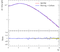
Figure 1: Validation against MCFM for $WZ$ production: $\Delta y$ between $W$ and $Z$ boson.

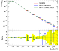
Figure 2: Validation against MCFM for $t\bar{t}$ production: $p_{T}$ of the top antiquark.

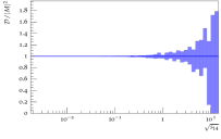
Figure 3: Real emission subtraction check for $Z+$jet production: singularity cancellation in $u\bar{u}\rightarrow e^{+}e^{-}gg$.

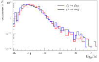
Figure 4: Pole cancellation check for $3$jet production: $\frac{1}{\varepsilon}$-pole cancellation.

5.2 A more concrete example: $t\bar{t}$ Production

Figs. 5 and 6 show validation plots for various matrix element providers against results obtained from MCFM, for $t\bar{t}$ production at NLO. Fig. 7 shows results for $t\bar{t}$ production at NLO, supplemented with the angular-ordered shower of Herwig and subtractive matching.

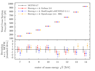
Figure 5: Comparison of total cross sections for $pp\rightarrow t\bar{t}$ at NLO. Various matrix element providers against MCFM. Fixed scale $\mu=\mu_{F}=\mu_{R}=80$ GeV. CT10nlo PDF set, $\alpha_{s}(M_{Z})|_{\rm{CT10nlo}}$. $M_{t}=173.5$ GeV, on-shell.

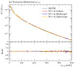
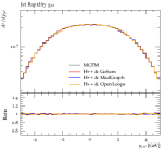
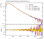
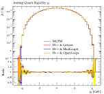
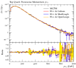
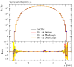
Figure 6: Comparison of various distributions for $pp\rightarrow t\bar{t}$ at NLO, at $14$ TeV. Various matrix element providers against MCFM. Fixed scale $\mu=\mu_{F}=\mu_{R}=80$ GeV. CT10nlo PDF set, $\alpha_{s}(M_{Z})|_{\rm{CT10nlo}}$. $M_{t}=173.5$ GeV, on-shell.

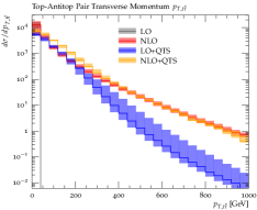
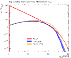
Figure 7: $pp\rightarrow t\bar{t}$ NLO matched, at $14$ TeV. MC@NLO–like matching to the angular ordered $\tilde{q}$–shower. Shower start scale $Q^{2}=\mu^{2}$. Hard scale variation: $\mu^{2}=\mu_{F}^{2}=\mu_{R}^{2}$ by factors of $0.5$ and $2$, where $\mu^{2}=\mu_{\min_{t\bar{t}}\{m_{T}\}}^{2}=\min_{i=t,\bar{t}}\left(m_{i}^{2}+p_{T,i}^{2}\right)$.

5.3 Data Comparison and Comparison vs. Herwig++ 2.7

In figs. 9 to 11 a small sample of results is shown that have been improved in the new release of Herwig 7.0 in contrast to the previous Herwig++ version 2.7. The following is just a small selection of distributions that have been checked against data. More will be shown in a series of upcoming papers. The Monte Carlo results from Herwig++ 2.7 use leading order plus parton shower, those from Herwig 7.0 use the angular-ordered parton shower (LO $\oplus$ PS), the angular-ordered parton shower supplemented by the built-in Powheg correction, which includes QCD and QED corrections for the case of $e^{+}e^{-}\to q\bar{q}$ (QCD $\otimes$ QED $\otimes$PS), by the automatically-calculated by Matchbox subtractive (MC@NLO-type) matching (NLO $\oplus$ PS) and multiplicative (Powheg-type, NLO $\otimes$ PS) corrections and, finally, the dipole shower supplemented by a subtractive matching to NLO cross sections (NLO $\oplus$ Dipoles).

Fig. 9 shows the thrust distribution at LEP, in comparison with data from ALEPH [42]. A long-standing problem of Herwig++ (producing too many very hard events, whether or not NLO matching was used) has been been solved by the improvements to the angular-ordered parton shower: all of the variants of NLO matching give a similar description of the data. In Fig. 9, the effect of the inclusion of photon emission in the angular-ordered parton shower is shown. Events at $z_{\gamma}=1$ are isolated photons (“jets” for which all of the jet energy is carried by a single photon), while events at lower $z_{\gamma}$ come from hard collinear photon emission from the final state quark jets. We see clearly that the results from Herwig++ have no component at large $z_{\gamma}$ at all, while all of the Herwig 7.0 variants are much closer to the data.

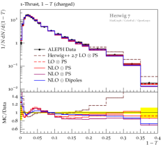
Figure 8: The thrust distribution in $\mathrm{e^{+}e^{-}}$ annihilation at $\sqrt{s}=M_{z}$, in comparison with ALEPH data [42].

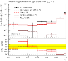
Figure 9: The distribution of photon-jet energy fraction in three-jet $\mathrm{e^{+}e^{-}}$ events at $\sqrt{s}=M_{z}$ defined with a cutoff in the $k_{\perp}$ algorithm of $y=0.1$ in comparison with ALEPH data [43].

Fig. 11 shows results for $\mathrm{Z+jets}$ production at the LHC, more concretely the distribution of separation in azimuthal angle between the $\mathrm{Z}$ boson and the hardest jet. The region $\Delta\phi\sim\pi$ corresponds to leading order kinematics, in which the $\mathrm{Z}$ boson gains transverse momentum by recoiling against a single hard parton, whereas the spectrum of events down to $\Delta\phi=0$ corresponds to events in which the $\mathrm{Z}$ boson recoils against two or more jets. The need for NLO corrections is clearly seen. An important cross-check of the two different automated NLO matching schemes and the two different shower algorithms, both using subtractive matching, can also be seen. In Fig. 11 the jet activity in $\mathrm{t\bar{t}}$ events at the LHC is shown, as revealed by the gap fraction. Herwig++ 2.7 is seen to have far too little jet activity (too many gap events). While Herwig 7.0 with the shower alone is somewhat closer to the data at small $Q_{\mathrm{sum}}$, a clear deficit is seen for hard jet events at high $Q_{\mathrm{sum}}$, while both the NLO matching schemes describe the data well.

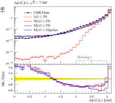
Figure 10: The distribution of separation in azimuthal angle between the $\mathrm{Z}$ boson and the hardest jet in $\mathrm{Z+jets}$ events in $\mathrm{pp}$ collisions at $\sqrt{s}=7\,\mathrm{TeV}$ in comparison with CMS data [44].

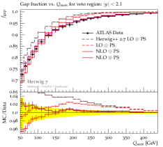
Figure 11: The fraction of events that have less than $Q_{\mathrm{sum}}$ transverse energy in the rapidity region $|y|<2.1$ in top quark-antiquark events in $\mathrm{pp}$ collisions at $\sqrt{s}=7\,\mathrm{TeV}$ in comparison with ATLAS data [45].

6 Summary and Outlook

The Herwig event generator has expanded its range of applicability to a multitude of underlying hard processes at NLO QCD, and a new version has recently been released [1]. Much of the new development is due to the Matchbox framework for fully automated NLO calculations and matching, which, however, also triggered crucial improvements to hitherto existing structures. The new release is the first major release in the new Herwig 7 series, which supersedes the capabilities of both its predecessors in the Herwig++ 2 [2, 3] and HERWIG 6 [4] series. Further physics related studies adressed by the new version, as well as comparisons with other event generator programs such as Pythia [46, 47] or Sherpa [48], will be covered in subsequent publications. Future development, for which the recent release forms the basis, includes LO and NLO multijet merging as well as the automation of NLO electroweak corrections.

References

- [1] J. Bellm et al., Herwig 7.0 / Herwig++ 3.0 Release Note, arXiv:1512.0117.
- [2] M. Bähr et al., Herwig++ Physics and Manual, Eur. Phys. J. C58 (2008) 639–707, [arXiv:0803.0883].
- [3] J. Bellm et al., Herwig++ 2.7 Release Note, arXiv:1310.6877.
- [4] G. Corcella et al., HERWIG 6: An event generator for Hadron Emission Reactions with Interfering Gluons (including supersymmetric processes), JHEP 01 (2001) 010, [hep-ph/0011363].
- [5] S. Gieseke, P. Stephens, and B. Webber, New Formalism for QCD Parton Showers, JHEP 12 (2003) 045, [hep-ph/0310083].
- [6] S. Plätzer and S. Gieseke, Coherent Parton Showers with Local Recoils, JHEP 01 (2011) 024, [arXiv:0909.5593].
- [7] S. Frixione and B. R. Webber, Matching NLO QCD Computations and Parton Shower Simulations, JHEP 06 (2002) 029, [hep-ph/0204244].
- [8] P. Nason, A new method for combining NLO QCD with shower Monte Carlo algorithms, JHEP 11 (2004) 040, [hep-ph/0409146].
- [9] S. Plätzer and S. Gieseke, Dipole Showers and Automated NLO Matching in Herwig++, Eur. Phys. J. C72 (2012) 2187, [arXiv:1109.6256].
- [10] S. Catani and M. H. Seymour, A General algorithm for calculating jet cross-sections in NLO QCD, Nucl. Phys. B485 (1997) 291–419, [hep-ph/9605323]. [Erratum: Nucl. Phys. B510 (1998) 503].
- [11] S. Catani, S. Dittmaier, M. H. Seymour, and Z. Trocsanyi, The dipole formalism for next-to-leading order QCD calculations with massive partons, Nucl. Phys. B627 (2002) 189–265, [hep-ph/0201036].
- [12] A. Bierweiler, T. Kasprzik, and J. H. Kühn, Vector-boson pair production at the LHC to accuracy, JHEP 1312 (2013) 071, [arXiv:1305.5402].
- [13] A. Bierweiler, T. Kasprzik, J. H. Kühn, and S. Uccirati, Electroweak corrections to W-boson pair production at the LHC, JHEP 11 (2012) 093, [arXiv:1208.3147].
- [14] S. Gieseke, T. Kasprzik, and J. H. Kühn, Vector-boson pair production and electroweak corrections in HERWIG++, Eur. Phys. J. C74 (2014) 2988, [arXiv:1401.3964].
- [15] T. Binoth et al., A Proposal for a standard interface between Monte Carlo tools and one-loop programs, Comput. Phys. Commun. 181 (2010) 1612–1622, [arXiv:1001.1307]. [,1(2010)].
- [16] S. Alioli et al., Update of the Binoth Les Houches Accord for a standard interface between Monte Carlo tools and one-loop programs, Comput. Phys. Commun. 185 (2014) 560–571, [arXiv:1308.3462].
- [17] J. R. Andersen et al., Les Houches 2013: Physics at TeV Colliders: Standard Model Working Group Report, arXiv:1405.1067.
- [18] G. Cullen et al., GoSam-2.0: a tool for automated one-loop calculations within the Standard Model and beyond, Eur. Phys. J. C74 (2014) 3001, [arXiv:1404.7096].
- [19] S. Badger, B. Biedermann, P. Uwer, and V. Yundin, Numerical evaluation of virtual corrections to multi-jet production in massless QCD, Comput. Phys. Commun. 184 (2013) 1981–1998, [arXiv:1209.0100].
- [20] F. Cascioli, P. Maierhofer, and S. Pozzorini, Scattering Amplitudes with Open Loops, Phys. Rev. Lett. 108 (2012) 111601, [arXiv:1111.5206].
- [21] K. Arnold et al., VBFNLO: A Parton level Monte Carlo for processes with electroweak bosons, Comput. Phys. Commun. 180 (2009) 1661–1670, [arXiv:0811.4559].
- [22] J. Baglio et al., Release Note - VBFNLO 2.7.0, arXiv:1404.3940.
- [23] J. Alwall, M. Herquet, F. Maltoni, O. Mattelaer, and T. Stelzer, MadGraph 5 : Going Beyond, JHEP 1106 (2011) 128, [arXiv:1106.0522].
- [24] J. Alwall et al., The automated computation of tree-level and next-to-leading order differential cross sections, and their matching to parton shower simulations, JHEP 07 (2014) 079, [arXiv:1405.0301].
- [25] M. Sjödahl, ColorFull – a C++ library for calculations in SU(Nc) color space, Eur. Phys. J. C75 (2015) 236, [arXiv:1412.3967].
- [26] S. Plätzer, Summing Large- Towers in Colour Flow Evolution, Eur. Phys. J. C74 (2014) 2907, [arXiv:1312.2448].
- [27] S. Plätzer, ExSample: A Library for Sampling Sudakov-Type Distributions, Eur. Phys. J. C72 (2012) 1929, [arXiv:1108.6182].
- [28] I. G. Knowles, Spin Correlations in Parton-Parton Scattering, Nucl. Phys. B310 (1988) 571.
- [29] I. G. Knowles, A Linear Algorithm for Calculating Spin Correlations in Hadronic Collisions, Comput. Phys. Commun. 58 (1990) 271–284.
- [30] J. C. Collins, Spin Correlations in Monte Carlo Event Generators, Nucl. Phys. B304 (1988) 794.
- [31] P. Richardson, Spin Correlations in Monte Carlo Simulations, JHEP 11 (2001) 029, [hep-ph/0110108].
- [32] M. Gigg and P. Richardson, Simulation of Beyond Standard Model Physics in Herwig++, Eur. Phys. J. C51 (2007) 989–1008, [hep-ph/0703199].
- [33] L. A. Harland-Lang, A. D. Martin, P. Motylinski, and R. S. Thorne, Parton distributions in the LHC era: MMHT 2014 PDFs, Eur. Phys. J. C75 (2015) 204, [arXiv:1412.3989].
- [34] S. Dulat et al., The CT14 Global Analysis of Quantum Chromodynamics, arXiv:1506.0744.
- [35] NNPDF Collaboration, R. D. Ball et al., Parton distributions for the LHC Run II, JHEP 04 (2015) 040, [arXiv:1410.8849].
- [36] G. P. Lepage, VEGAS: An Adaptive Multi-dimensional Integration Program, 1980. CLNS-80/447.
- [37] F. Campanario, T. M. Figy, S. Plätzer, and M. Sjödahl, Electroweak Higgs Boson Plus Three Jet Production at Next-to-Leading-Order QCD, Phys. Rev. Lett. 111 (2013) 211802, [arXiv:1308.2932].
- [38] R. Frederix and S. Frixione, Merging meets matching in MC@NLO, JHEP 12 (2012) 061, [arXiv:1209.6215].
- [39] R. Frederix, S. Frixione, A. Papaefstathiou, S. Prestel, and P. Torrielli, A study of multi-jet production in association with an electroweak vector boson, arXiv:1511.0084.
- [40] F. Goertz, A. Papaefstathiou, L. L. Yang, and J. Zurita, Higgs boson pair production in the D=6 extension of the SM, JHEP 04 (2015) 167, [arXiv:1410.3471].
- [41] P. Maierhöfer and A. Papaefstathiou, Higgs Boson pair production merged to one jet, JHEP 03 (2014) 126, [arXiv:1401.0007].
- [42] ALEPH Collaboration, R. Barate et al., Studies of quantum chromodynamics with the ALEPH detector, Phys. Rept. 294 (1998) 1–165.
- [43] ALEPH Collaboration, D. Buskulic et al., First measurement of the quark to photon fragmentation function, Z. Phys. C69 (1996) 365–378.
- [44] CMS Collaboration, S. Chatrchyan et al., Event shapes and azimuthal correlations in + jets events in collisions at TeV, Phys. Lett. B722 (2013) 238–261, [arXiv:1301.1646].
- [45] ATLAS Collaboration, G. Aad et al., Measurement of production with a veto on additional central jet activity in pp collisions at sqrt(s) = 7 TeV using the ATLAS detector, Eur. Phys. J. C72 (2012) 2043, [arXiv:1203.5015].
- [46] T. Sjöstrand, S. Mrenna, and P. Z. Skands, A Brief Introduction to PYTHIA 8.1, Comput. Phys. Commun. 178 (2008) 852–867, [arXiv:0710.3820].
- [47] T. Sjöstrand, S. Ask, J. R. Christiansen, R. Corke, N. Desai, P. Ilten, S. Mrenna, S. Prestel, C. O. Rasmussen, and P. Z. Skands, An Introduction to PYTHIA 8.2, Comput. Phys. Commun. 191 (2015) 159–177, [arXiv:1410.3012].
- [48] T. Gleisberg, S. Hoeche, F. Krauss, M. Schönherr, S. Schumann, F. Siegert, and J. Winter, Event generation with SHERPA 1.1, JHEP 02 (2009) 007, [arXiv:0811.4622].