The scaling window of the 5D Ising model with free boundary conditions

Abstract

The five-dimensional Ising model with free boundary conditions has recently received a renewed interest in a debate concerning the finite-size scaling of the susceptibility near the critical temperature. We provide evidence in favour of the conventional scaling picture, where the susceptibility scales as $O(L^{2})$ inside a critical scaling window of width $O(1/L^{2})$. Our results are based on Monte Carlo data gathered on system sizes up to $L=79$ (ca. three billion spins) for a wide range of temperatures near the critical point. We analyse the magnetisation distribution, the susceptibility and also the scaling and distribution of the size of the Fortuin-Kasteleyn cluster containing the origin. The probability of this cluster reaching the boundary determines the correlation length, and its behaviour agrees with the mean field critical exponent $\delta=3$, that the scaling window has width $O(1/L^{2})$.

I Introduction

The Ising model in dimension $d=5$ is of particular interest since it is the first case where the model is strictly above its upper critical dimension $d_{c}=4$. Rigorous results Aizenman (1982); Sokal (1979) establish that the critical exponents of the model assume their mean field values. Here the specific heat exponent $\alpha=0$, and the results of Sokal (1979) also imply that the specific heat is bounded at the critical point. Recent simulation results Lundow and Markström (2015a) also indicate that, just as for the mean field case, the specific heat is discontinuous at the critical point.

In contrast to these asymptotic results there has been a long running debate over the finite size scaling for the model with free boundary conditions. We’ll refer the reader to Berche et al. (2012) for a fuller overview of the history and stick to the presently most relevant parts here. For $d=5$ and cyclic boundary conditions there is agreement that e.g. $\chi\propto L^{5/2}$ for a lattice of side $L$. The conventional picture for the free boundary case is that $\chi\propto L^{2}$. However, it has also been suggested Berche et al. (2012) that the free boundary case should scale in the same way as the cyclic boundary case near the finite size susceptibility maximum. A computational study Lundow and Markström (2011) of the, then, largest lattices possible supported the conventional picture, but in Berche et al. (2012) it was suggested this was due to an underestimate of the influence of the large boundaries of the used systems. For systems exactly at the critical coupling this issue was resolved in Lundow and Markström (2014) where a study of systems up to $L=160$ demonstrated an increasingly good agreement with the conventional picture as the system size was increased. But, this left the behaviour in the rest of the critical scaling window open.

The aim of the current paper is to extend the study of large systems from Lundow and Markström (2014) to the full critical window, including the location of the maximum of $\chi$, and give the best possible estimates for the scaling behaviour in the coupling region discussed by all the previous papers. Apart from the susceptibility we also study properties of the Fortuin-Kasteleyn cluster containing the origin and use those to estimate both the susceptibility and the correlation length of the model.

To concretize, the predictions from Berche et al. (2012) are that the location of the maximum for $\chi$ will scale as $L^{-2}$ and the maximum value as $L^{5/2}$. The more recent Wittmann and Young (2014) agrees with these predictions, and also the prediction from Rudnick et al. (1985) that the location of the maximum of the susceptibility should scale as $L^{2}$, as does Flores-Sola et al. (2015), but both are based on smaller system sizes than those considered in the present work.

In short, our conclusion is that the data is well fitted by the conventional scaling picture, both for the location and value of the susceptibility, and location of the finite size critical point for the magnetization.

II Definitions and details

For a given graph $G$ on $N$ vertices the Hamiltonian with interactions of unit strength along the edges is $\mathcal{H}=-\sum_{ij}s_{i}s_{j}$ where the sum is taken over the edges $ij$. Here the graph $G$ is a $5$-dimensional grid graph of linear order $L$ with free boundary conditions, i.e. a cartesian product of $5$ paths on $L$ vertices, so that the number of vertices is $N=L^{5}$ and the number of edges is $5L^{5}(1-1/L)$. We use $K=1/k_{B}T$ as the dimensionless inverse temperature (coupling) and denote the thermal equilibrium mean by $\left\langle\cdots\right\rangle$. The critical coupling $K_{c}$ was recently estimated by us Lundow and Markström (2015a) to $K_{c}=0.11391498(2)$. We will define a rescaled coupling as $\kappa=L^{2}(K-K_{c})$ which gives a scaling window of width $O(1/L^{2})$. The standard definitions apply; the magnetisation is $M=\sum_{i}S_{i}$ (summing over the vertices $i$) and the energy is $E=\sum_{ij}S_{i}S_{j}$ (summing over the edges $ij$). We let $m=M/N$, $U=E/N$ and $\mathcal{U}=\left\langle U\right\rangle$.

The susceptibility is $\chi=\left\langle M^{2}\right\rangle/N$ while we define the modulus susceptibility as $\bar{\chi}=\mathrm{var}\!\left(|M|\right)/N$. The standard deviation is denoted $\sigma$, as is customary. We will refer to the point where the distribution of $M$ changes from unimodal to bimodal as $K^{*}_{c}(L)$, or, in its rescaled form, $\kappa^{*}_{c}(L)$. Recall also that thermodynamic derivatives of e.g. $\log\chi$ can be obtained through correlation measurements $\partial\log\left\langle|M|^{\ell}\right\rangle/\partial K=\left(\langle E\,|M|^{\ell}\rangle/\langle|M|^{\ell}\rangle\right)-\langle E\rangle$.

Let $\langle S\rangle$ denote the average size of a flipped cluster and recall Wolff (1989) that $\chi=\langle S\rangle$. We use the subscript $o$ to denote the origin (i.e. centre) vertex of the grid $G$ so that $\langle S_{o}\rangle$ is the average size of a cluster containing the origin. The event that a cluster containing the origin also reaches the boundary $\partial G$ of the graph is denoted $o\leftrightarrow\partial G$.

We have collected data using Wolff-cluster spin updating for $L=15$, $19$, $23$, $31$, $39$, $47$, $55$, $63$, $79$ for a wide and dense set of $\kappa$-values in $0\leq\kappa\leq 0.92$. The data include e.g. magnetisation, energy ($L\leq 63$), size and radius of the origin cluster. The total number of measurements range from about $300000$ for the small systems ($L\leq 39$) down to $100000$ for $L=63$ and $50000$ for $L=79$.

III The width of the scaling window and the shift exponents

We begin by establishing the natural width of the scaling window, i.e. the form of a natural rescaled temperature. We have already defined the rescaled coupling as $\kappa=L^{2}(K-K_{c})$ with the expectation that this will be the relevant scaling. In principle, the location of different effective finite size critical points could scale with different exponents and we will compare a number of such possibilities.

We used a 2nd order interpolation of the data points to estimate the location of the maximum for three different parameters: $\bar{\chi}$, $\partial\log\left\langle|m|\right\rangle/\partial K$ and $\partial\log\chi/\partial K$. For the last two we only have these data for $L\leq 63$. The locations are plotted versus $1/L$ in Figure 1. The values clearly point to three different limit $\kappa$-values. Based on $L\geq 19$ we estimate the limit values and an error bar by removing each of the data points in turn and fitting a line to the remaining points. Thus we find $\kappa_{c}(L)=0.8763(5)-1.21(2)/L$ for the $\bar{\chi}$-maximum, $\kappa_{c}(L)=0.8742(5)-1.49(1)/L$ for the maximum $\partial\left\langle|m|\right\rangle/\partial K$ and $0.8725(3)-1.50(1)/L$ for the maximum $\partial\log\chi/\partial K$. We conclude that our rescaled coupling $\kappa$ is the correct scaling, and each of the effective critical points scale with the same exponent.

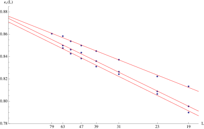
Figure 1: (Colour on-line) Location $\kappa_{c}(L)$ of the maximum $\bar{\chi}$, $\partial\log\left\langle|m|\right\rangle/\partial K$ and $\partial\log\chi/\partial K$ plotted against $1/L$ for $L=19$, $23$, $31$, $39$, $47$, $55$, $63$ and $79$ ($L=79$ only for $\bar{\chi}$). Fitted lines are respectively $0.8763-1.21x$, $0.8742-1.49x$ and $0.8725-1.50x$ (downwards in figure) where $x=1/L$.

IV The low and high-temperature regions

Next we estimate the location of the point where the magnetisation distribution switches from unimodal to bimodal, denoted $\kappa^{*}_{c}(L)$. This point will be seen as the effective finite size separator between the high and low-temperature regions of the model.

To do this we note that near this point the standardised distribution of $M$ (i.e. of $M/\sigma$ where $\sigma^{2}=\mathrm{var}\!\left(M\right)$) is well-fitted by the simple formula $f(x)=c_{0}\exp(c_{2}x^{2}+c_{4}x^{4})$. The lower inset of Figure 2 shows the distribution of $M/\sigma$ for $L=23$ at $\kappa=0.76$ ($K=0.11535165$) together with the fitted formula. The binning of the data was done with Mathematica’s built-in procedures but the results are not very sensitive to this choice. At this $\kappa$ (i.e. for $L=23$) the distribution is very close to shifting from unimodal to bimodal, as is indicated by the very small coefficient $c_{2}=-0.002735$. The distribution has kurtosis $2.2217$ and when $c_{2}=0$ the kurtosis becomes $\Gamma(1/4)^{4}/8\pi^{2}\approx 2.1884$. In fact, it works equally well to simply measure the kurtosis and then estimate through interpolation at which point the kurtosis is $2.1884$. All this suggests that the distribution’s shape is well captured by $f(x)$. See also Lundow and Markström (2015a) where we apply this formula to 5D grids with periodic boundary conditions.

The upper inset of Figure 2 shows the measured coefficient $c_{2}$ plotted against $\kappa$ for a range of $L$. The value of $c_{4}$ (not shown) at $\kappa^{*}_{c}(L)$ is somewhat noisy but it seems to converge to $-0.114(3)$. For a cyclic boundary this value is close to $-0.602$ Lundow and Rosengren (2013).

Figure 2 shows $\kappa^{*}_{c}(L)$ (where $c_{2}=0$) versus $1/L$. The fitted 2nd degree polynomial suggests $\kappa^{*}_{c}(L)=0.8561(6)-2.52(3)/L+7.6(4)/L^{2}$, with error bars obtained as above, so that $\kappa^{*}_{c}\approx 0.856$. This point then represents where the true low-temperature region begins.

The point $\kappa^{*}_{c}(L)$ constitutes an effective critical temperature but its scaling rule appears to depend strongly on the boundary conditions. Note that for periodic boundary conditions the corresponding point $K^{*}_{c}(L)$ converges to $K_{c}$ with rate $1/L^{3}$ Brezin and Zinn-Justin (1985), i.e. faster than the width of the scaling window, which is $1/L^{5/2}$ in that case. For free boundary conditions we instead see that $K^{*}_{c}(L)\to K_{c}$ with the same rate as the width of the scaling window, i.e. $1/L^{2}$.

We note that in Wittmann and Young (2014) an estimate based in the kurtosis was used, but instead of using the universal kurtosis-value given at the point where $c_{2}=0$ they hand picked a value for the kurtosis and then used the fact that all fixed such values should give the same scaling, with larger or smaller corrections to the scaling.

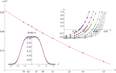
Figure 2: (Colour on-line) Effective critical temperature $\kappa^{*}_{c}(L)$ (where $c_{2}=0$) versus $1/L$ for $L=15$, $19$, $23$, $31$, $39$, $47$, $55$, $63$, $79$. The fitted curve is $0.856-2.52x+7.6x^{2}$ where $x=1/L$. Lower inset: Probability density function $\Pr(M/\sigma)$ (dots) for $L=23$ at $\kappa=0.76$ ($K=0.11535165$). Fitted (red) curve is $0.3223\exp(-0.002735x^{2}-0.1164x^{4})$. Upper inset: Coefficient $c_{2}$ of the fitted density function $f(x)$ plotted versus $\kappa$ for $L=15$, $19$, $23$, $31$, $39$, $47$, $55$, $63$, $79$ (left to right).

V Scaling of susceptibility

Let us now return to the matter of the finite-size scaling of $\chi$ and $\bar{\chi}$. With the onset of the low-temperature region at (asymptotically) $\kappa^{*}_{c}=0.856$ we look at the scaling behaviour of $\chi$ at fixed $\kappa$ below and above this point. Consider Figure 3 where we show $\chi/L^{2}$ versus $L$ for six different fixed $\kappa$-values. Lines are fitted on $L\geq 31$ to demonstrate the presence of correction terms. The behaviour is clearly linear for larger $L$, with the possible exception of $\kappa=0.86$, i.e. above $\kappa^{*}_{c}=0.856$ where we have entered the low-temperature region and have a bimodal magnetization, but even here the correction term is still rather weak. However, higher $\kappa$-values render us stronger corrections. The normalised susceptibility was also used in Wittmann and Young (2014), but there the estimates, which lead to scaling proportional to $L^{5/2}$ were based on much smaller lattices $L\leq 36$, where finite size effects are much stronger.

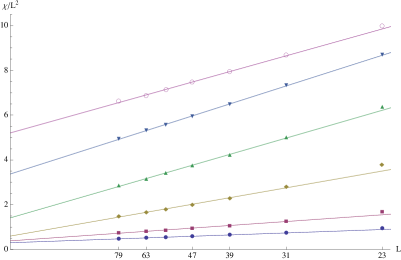
Figure 3: (Colour on-line) Normalised susceptibility $\chi/L^{2}$ at fixed $\kappa$ versus $1/L$ for $L=23$, $31$, $39$, $47$, $55$, $63$, $79$ at $\kappa=0.70$, $0.75$, $0.80$, $0.83$, $0.85$, $0.86$ (upwards). The lines are fitted on $L\geq 31$. Error bars are smaller than the points.

Moving on to the modulus susceptibility $\bar{\chi}/L^{2}$ the corrections become clear and present, even for $\kappa\leq 0.856$, but never more than can be captured by a simple 2nd degree polynomial. Figure 4 shows this effect. Note also that once we have gone beyond the maximum at $\kappa=0.876$ the behavior quickly becomes linear again as is clearly seen at $\kappa=0.92$, which is where our data end. Combining all the measured $\bar{\chi}/L^{2}$ with their asymptotic values, based on 2nd degree polynomials fitted on $L\geq 31$, we now obtain Figure 5.

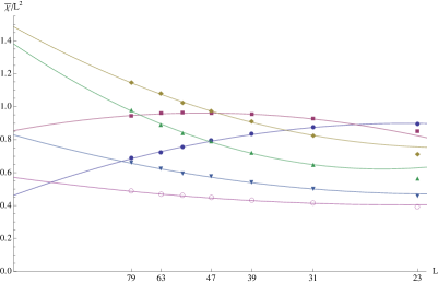
Figure 4: (Colour on-line) Normalised modulus susceptibility $\bar{\chi}/L^{2}$ at fixed $\kappa$ versus $1/L$ for $L=23$, $31$, $39$, $47$, $55$, $63$, $79$ at $\kappa=0.82$, $0.84$, $0.86$, $0.88$, $0.90$ and $0.92$. Downwards at $y$-axis is $\kappa=0.86$, $0.88$, $0.84$, $0.90$, $0.92$, $0.82$. The 2nd degree curves are fitted on $L\geq 31$. Error bars are smaller than the points.

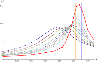
Figure 5: (Colour on-line) Normalised modulus susceptibility $\bar{\chi}/L^{2}$ versus $\kappa$ for $L=15$, $19$, $23$, $31$, $39$, $47$, $55$, $63$, $79$. The thick red curve is the estimated limit found by fitting a 2nd degree polynomial in $1/L$ to the data points for $L\geq 31$ at each fixed $\kappa$. The left vertical line at $\kappa=0.856$ (orange) indicates where the magnetisation distribution becomes bimodal when $L\to\infty$. The right vertical line at $\kappa=0.877$ (blue) is where the maximum $\bar{\chi}/L^{2}$ is located when $L\to\infty$.

For this range of lattice sizes and at least some values of $\kappa$ one can make a reasonable fit to the data with a $L^{5/2}$ scaling as well, by including sufficient correction terms. But, as we can see in Figure 5, the $L^{2}$ scaling gives values that decrease to their limit value for a large range of $\kappa$, possibly all $\kappa$ below $\kappa^{*}_{c}$, making an even larger power of $L$ seem unlikely here.

VI The FK-cluster at the origin

Our next object of study is the Fortuin-Kasteleyn cluster containing the origin. This is the cluster which the Wolff random cluster algorithm builds when started at the central vertex of our lattice, and is one of the clusters in the FK-random cluster representation of the Ising model. From the FK-model the usual susceptibility can be computed as the expected cluster size, and with free boundary the expected size of the origin cluster will be larger than the average cluster size, thereby giving an upper bound on the susceptibility. This observation was used in Lundow and Markström (2014) to give a susceptibility estimate which was hoped to be less affected by the effects of the free boundary, in part as a response to the truncation method of Berche et al. (2012).

As described we expect $\langle S_{o}\rangle$ to place an upper bound on $\chi$, but we do not expect them to be of different scaling orders. Plotting $\langle S_{o}\rangle/L^{2}$ versus $1/L$ demonstrates a similar behaviour to that of $\chi/L^{2}$. In Figure 6 we show the scaling at a number of different $\kappa$-values below $\kappa^{*}_{c}$. In fact, a strong correction enters the picture already at $\kappa=0.85$ (not shown in the figure). This is to be expected since above $\kappa^{*}_{c}$ there are additional terms from the FK-model affecting the Ising susceptibility, and those are not included in our sampled data.

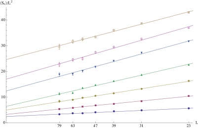
Figure 6: (Colour on-line) Normalised size of origin cluster $\langle S_{o}\rangle/L^{2}$ at fixed $\kappa$ versus $1/L$ for $L=23$, $31$, $39$, $47$, $55$, $63$, $79$ at $\kappa=0.70$, $0.75$, $0.78$, $0.80$, $0.82$, $0.83$ and $0.84$ (upwards). Lines fitted on $L\geq 23$.

The distribution of the origin cluster size $S_{o}$ is also an interesting object. It is a Pareto-like distribution with density proportional to $x^{-1-1/\delta}$, or, by definition Grimmett (2004),

$$\Pr(S_{o}\leq x)=1-x^{-1/\delta}$$ (1)

where $\delta$ is the critical exponent reflecting how an external field affects the magnetisation at the critical temperature, here having the mean field value $\delta=3$.

In Figure 7 we show a log-log plot of the distribution density (for small $x=S_{o}$) together with a line having slope $-4/3$, consistent with $\delta=3$. The line is clearly an excellent fit. The plot shows the distribution for $L=63$ at $\kappa=0.85$ but for this range of cluster sizes the plot is indistinguishable from that of other $\kappa$-values, and indeed of other $L$ (except the smallest $L$).

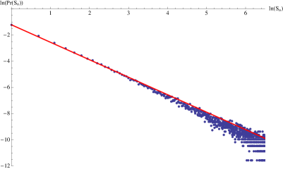
Figure 7: (Colour on-line) Log-log plot of the size distribution of the origin cluster for $L=63$ and $\kappa=0.85$. The red line has slope $-4/3$.

VII Correlation length

The origin cluster can also be used to estimate the correlation length of the model. In the high temperature region the correlation length $\xi$ is given, see Grimmett (2004), by the limit

$$\frac{1}{\xi}=\lim_{L\to\infty}\frac{-\log\Pr(o\leftrightarrow\partial G)}{L}$$ (2)

For a fixed $\kappa$ we expect not just $\xi\to\infty$, but rather that the correlation length is comparable to $L$, i.e. $\xi/L\to a(\kappa)$ for some function $a$. Thus we propose to estimate $a(\kappa)$ by first defining $\xi/L=-1/\log\Pr(o\leftrightarrow\partial G)$ and then use a simple projection rule to estimate the limit function $a(\kappa)$.

The inset of Figure 8 shows $\xi/L$ versus $1/L$ for a range of $L$ at different $\kappa$-values. Figure 8 also shows a rough estimate of $a(\kappa)$ based upon fitted 2nd degree polynomials (on $L\geq 15$) for each $\kappa$. We expect the errors in the plot to be significant although the general behaviour as such is correct. In the low-temperature region the identity in Equation 2 is no longer valid, and the probability that the origin cluster reaches the boundary tends to 1, and this agrees well with the steep growth beginning at $\kappa\approx 0.85$, the start of the effective finite size low-temperature region.

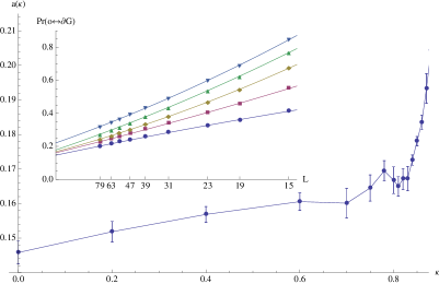
Figure 8: (Colour on-line) Correlation coefficient $a(\kappa)$ versus $\kappa$ based on fitted 2nd degree polynomials for $L\geq 15$ (see text). Note the sudden growth that sets in near $\kappa=0.85$. Inset: $\xi/L$ plotted against $1/L$ for $L=23$, $31$, $39$, $47$, $55$, $63$ and $79$ at at $\kappa=0$, $0.40$, $0.70$, $0.80$, $0.84$, $0.88$ and $0.92$ (upwards). Curves are 2nd degree polynomials fitted to $15\leq L\leq 79$.

VIII Conclusions

As we have seen here our data fits excellently with the conventional scaling picture for the free boundary case. Now, apart from this fact we believe that there are good reasons for expecting distinct behaviour from the free and cyclic boundary cases. As is well known the Ising model is equivalent to the Fortuin-Kasteleyn random cluster model for $q=2$. The case $q=1$ corresponds to ordinary percolation and $q\rightarrow 0$ gives the random spanning tree for the lattice.

For the random spanning tree Pemantle Pemantle (1991) proved that for large enough $d$ the distance between two points in the tree scales as $L^{2}$ with free boundary and as $L^{d/2}$ with cyclic boundary. For percolation, Aizenmann Aizenman (1997) conjectured that for large enough $d$ the size of the largest cluster should scale as $L^{4}$ with free boundary and $L^{2d/3}$ with cyclic boundary. This conjecture was later proven in Heydenreich and van der Hofstad (2007, 2011). So, for both $q=0$ and $q=1$ we have rigorous results showing that free and cyclic boundary conditions lead to distinct scalings.

Aizenman’s conjectured scaling $L^{2d/3}$ came from the fact that the cyclic boundary case was expected to behave like the critical Erdős-Renyi random graph, where the maximum cluster has size $N^{2/3}$, where $N$ is the number of vertices, which would be $L^{d}$ for the lattice. Again, there are detailed rigorous results Luczak and Luczak (2006) concerning the random cluster model on the complete graph and in Lundow and Markström (2015b) it was demonstrated that Monte Carlo data for the FK-model with $q=2$ and $d=5$ with cyclic boundary gives a detailed agreement with the scaling for the complete graph. In particular, the size of the largest cluster has the same scaling for both graphs for several different rescaled coupling ranges.

Now, the $L^{2}$ scaling observed in this paper for the origin cluster can be seen as an indicator of the correct scaling of the largest cluster as well. This would give a scaling which is different for the free and cyclic boundary cases, just as one would expect from the known results for lower $q$. In Lundow and Markström (2011) the authors conjectured that for every $q$ there is a $d(q)$ such that above this dimension the FK-model with cyclic boundary behaves like the model on a complete graph, giving a partial generalisation of Aizenmann’s conjecture for all $q$. In fact, we also expect the model with free boundary to follow a simpler mean-field scaling, similar to that seen on an infinite tree, or Bethe lattice. The fact that there are several distinct basic model systems, e.g. the complete graphs and the Bethe lattices, which on one hand have mean field critical exponents but on the other hand differ on more detailed properties is probably under-appreciated in the older literature.