FRB repetition and non-Poissonian statistics

Abstract

We discuss some of the claims that have been made regarding the statistics of fast radio bursts (FRBs). In an earlier paper (Connor et al., 2015) we conjectured that flicker noise associated with FRB repetition could show up in non-cataclysmic neutron star emission models, like supergiant pulses. We show how the current limits of repetition would be significantly weakened if their repeat rate really were non-Poissonian and had a pink or red spectrum. Repetition and its statistics have implications for observing strategy, generally favouring shallow wide-field surveys, since in the non-repeating scenario survey depth is unimportant. We also discuss the statistics of the apparent latitudinal dependence of FRBs, and offer a simple method for calculating the significance of this effect. We provide a generalized Bayesian framework for addressing this problem, which allows for direct model comparison. It is shown how the evidence for a steep latitudinal gradient of the FRB rate is less strong than initially suggested and simple explanations like increased scattering and sky temperature in the plane are sufficient to decrease the low-latitude burst rate, given current data. The reported dearth of bursts near the plane is further complicated if FRBs have non-Poissonian repetition, since in that case the event rate inferred from observation depends on observing strategy.

1 Introduction

There is mounting evidence that the new class of transients known as fast radio bursts (FRBs) are of extraterrestrial origin. The most striking features of FRBs are their large dispersion measures (DMs) – too high to be attributed to our own Galaxy’s interstellar medium (ISM) – and their event rate (10³-$10^{4}$ sky^-1 day^-1). They last for about a millisecond with peak flux of roughly a Jy, and none has been conclusively shown to repeat. This has led to the interpretation that FRBs are cosmological, since the intergalactic medium (IGM) would naturally provide DMs between 300-1600 pc cm^-3 for sources at $z\sim 0.3$-$1$ (Thornton, 2013).

Given their apparent phenomenological richness (polarization, scattering, etc.) and considering how little we know about their location and physical origin, it is likely that FRBs will be of interest to the community for years to come, assuming they are not terrestrial. Though we are in the regime of only a dozen published FRBs, at present the conventional wisdom is that they are likely cosmological in origin (Thornton, 2013), they seem to not repeat regularly (Petroff et al., 2015), and there is a dearth of bursts at low Galactic latitudes (Petroff et al., 2014; Burke-Spolaor & Bannister, 2014; Macquart & Johnston, 2015).

Based on this premise there have been a number of models proposed to describe cataclysmic, cosmological FRBs (Mickaliger et al., 2012; Totani, 2013; Falcke & Rezzolla, 2014; Mingarelli et al., 2015). However since the field is still in its infancy it is important to leave as many conceptual doors open as possible; assumptions about the statistics of the event rate, spatial distribution, and repetition are important for the design and observing strategy of upcoming surveys. In Section 2 we explore the consequences of repeating FRBs in the case where their burst rate is non-Possionian and exhibits a 1/$f$ power spectrum, or pink noise. We also investigate the claims of Maoz et al. (2015) that FRB 140514 could have been the same source as FRB 110220, and comment on its implications. In Section 3 we discuss the impact of FRB repetition on survey strategy. In Section 4 we discuss the statistical treatment of the apparent latitudinal dependence of the event rate and the lack of detections at low Galactic latitude.

2 Repeat rates

Though no source has been shown with certainty to repeat, the limits on repeatability of FRBs are still weak. Several models generically predict repetition, whether periodic or stochastic. Galactic flaring stars (Maoz et al., 2015), radio-bursting magnetars (Popov & Postnov, 2007; Pen & Connor, 2015), and pulsar planet systems (Mottez & Zarka, 2014) all predict repetition with varying rates and burst distributions.

In Connor et al. (2015) it was suggested that supergiant pulses from very young pulsars in supernova remnants of nearby galaxies could explain the high DMs, Faraday rotation, scintillation, and polarization properties of the observed FRBs. We proposed that if the repetition of supergiant pulses were non-Poissonian (with a pink or red distribution) then one might expect several bursts in a short period of time. It is also worth mentioning that the statistics and repeat rates of FRBs could vary from source to source – even if they come from a single class of progenitors – so a long follow-up on an individual burst may not provide global constraints. In this letter we will refer to stationary Poisson processes (expectation value, $\mu(t)$, is constant in time) as “Poissonian”. When we discuss non-Poissonian statistics we will be focusing on stochastic processes that are correlated on varying timescales. For example we will not discuss periodic signals, which are not Poissonian but have already been studied (Petroff et al., 2015).

2.1 Flicker noise

Pink noise is ubiquitous in physical systems, showing up in geology and meteorology, a number of astrophysical sources including quasars and the sun, human biology, nearly all electronic devices, finance, and even music and speech (Press, 1978; Voss & Clarke, 1975). Though there is no agreed-upon mathematical explanation for this phenomenon (Milotti, 2002), fluctuations are empirically known to be inversely proportional to frequency for a variety of dynamical systems. This can be written as

$$S(f)=\frac{C}{f^{\gamma}}\,\,\,\,\,\ \textup{if}\,\,\,\,\,f_{\rm{min}}\leq f\leq f_{\rm{max}},$$ (1)

where $S(f)$ is the spectral density (i.e. power spectrum), $\gamma$ is typically between 0.5-2, and $f_{\rm{min}}$ and $f_{\rm{max}}$ are cutoffs beyond which the power law does not hold. In this paper will describe these distributions as having flicker noise.

In the case of a time-domain astronomical source, this results in uniformity on short timescales, i.e. a burst of clustered events followed by extended periods of quiescence. If FRBs were to exhibit such flicker noise then their repetition would not only be non-periodic, but would also have a time-varying pulse rate and, more importantly, variance. Therefore the number of events seen in a follow-up observation would depend strongly on the time passed since the initial event.

In Petroff et al. (2015) the fields of eight FRBs discovered between 2009 and 2013 were followed up from April to October of 2014, for an average of 11.4 hours per field. During this follow-up programme FRB 140514 was found in the same beam as FRB 110220, however the authors argue that it is likely a new source due to its lower DM. After its discovery, the field of 140514 was monitored five more times, starting 41 days later on 2014-06-24, without seeing anything. Under the assumption that 140514 was a new FRB that only showed up in the same field coincidentally and that the repeat rate is constant, Petroff et al. (2015) rule out repetition with a period $P\leq$ 8.6 hours and reject 8.6 $<$ $P$ $<$ 21 hours with 90$\%$ confidence. However it is possible that one or both of those premises is invalid, so it is useful to explore the possibility of non-stationary repeat rate statistics and repeating FRBs with variable DM.

If the statistics of the FRB’s repeat rate were non-Poissonian and initial bursts from FRBs were to have aftershocks similar to earthquakes, then the non-immediate follow-up observations impose far weaker repeat rate limits than has been suggested. We constructed a mock follow-up observation of the eight FRBs whose fields were observed in Petroff et al. (2015). We then asked how many bursts are seen to repeat if we do an immediate follow-up vs. a follow-up several years after the initial event at times corresponding to the actual observations carried out.

We run a simple Monte Carlo simulation with one sample per hour and a probability of 0.5 that a given sample has a burst in it. The repeat rate of once per two hours is chosen arbitrarily and should not affect the comparison. To get the 1$/f^{\gamma}$ distribution we take an uncorrelated Gaussian time stream centred on 0 and move to Fourier space, then multiply by $f^{\gamma/2}$, which gives a power spectrum with the desired shape. We then inverse Fourier transform back to get the pink or red time stream. We then take samples with a positive value to contain a pulse and samples with a negative value to contain none.. In the stationary Poisson case, the rate of bursts in the immediate follow-up is the same as the multi-year follow-up since all times are statistically equivalent. However with flicker noise the variance is strongly time-dependent. If we imagine an object that repeated on average once per two hours, then if those pulses were Poisson-distributed the probability of seeing zero bursts in 11.4 hours or longer is $\sim 0.007$. With pink noise one expects this roughly 20$\%$ of the time, since the system prefers either to be in “on” or “off” mode. If the average repeat period were more like 5-20 hours, then we would often see nothing in a multi-day follow-up observation that took place weeks or years after the initial event.

This is consistent with what Petroff et al. (2015) saw, though the conclusions differ depending on the assumed statistics. In Figure 1 we show a sample from this simulation for three repeat distributions. The right panel shows how, if an FRB’s burst rate has long-term correlations (1$/f^{\gamma}$), the likelihood of a repeat is greatly increased if the follow-up observation is immediately after the initial event, rather than months or years after.

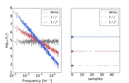
Figure 1: Realization of our mock follow-up Monte Carlo. Left panel: Power spectrum for pulse arrival times of a single FRB. Grey shows a flat spectrum, corresponding to the often assumed Poissonian repetition rate. The red and blue spectra show flicker noise, with pink (1/$f$) noise and Brownian (1/$f^{2}$) noise respectively. Right panel: We found the first “event” in our Monte Carlo (represented by a star) for the three different spectra and plotted their behaviour in the subsequent 48 hours of follow-up. Though the average probability over the whole simulation is 0.5 for each distribution, when we zoom in on this short period the strong time-like correlations in the $1/f^{\gamma}$ cases means there are many repetitions: they are in an “on” state at this time.

2.2 FRBs 110220 and 140514

Using the event rate of roughly $10^{4}$ sky^-1 day^-1 from Thornton (2013), it was originally reported that the probability of seeing a new FRB in the field of 110220 during the 85 hours of follow-up was $0.32$ (Petroff et al., 2015). It was then pointed out by Maoz et al. (2015) that this underestimated the coincidence by an order of magnitude, since they estimated the rate in any one of the 13 beams, while the new event occurred in the identical beam. The probability also dropped due to the updated daily event rate, given the Thornton (2013) estimate is now thought likely to be too high. In general we expect the true rate of FRBs to be lower than what is reported due to non-publication bias: If archival data are searched and nothing is found, it is less likely to be published than if something is found. That said, using the rate calculated by Rane et al. (2015) and following the procedure of Maoz et al. (2015), we find the likelihood of finding a new burst to be between 0.25-2.5$\%$.

Given the relatively low probability of finding a new FRB in the same field and since there are models that predict burst repetition with variable DMs (Connor et al., 2015; Maoz et al., 2015) one can ask the question: If one FRB out of eight is found to repeat during 110 hours of follow-up (including extra time spent on 140514), what are the limits on the average repeat period? Another way of asking this question is what is the probability of some number of repetitions during the 110 hours, given a repeat rate. The answer to this question depends strongly on the power spectrum’s shape. For the sake of example, if the average repeat rate is once per two hours, then the probability of one repeat or fewer in the Poisson case is effectively zero. With a pink distribution it is closer to $5\%$, even though the expected number would be 55. This is shown in Figure 2, in which we plot the probability of seeing zero or one repeat burst (the two options for FRB 140514), given some average repetition period, $P$. We generate the pink distribution in the same way described in Section 2.1, using one-hour samples and a long-wavelength cutoff at 1.2 million hours. Though it was taken arbitrarily, the probability of seeing no bursts should depend only weakly on this cutoff. Since the variance scales logarithmically with this number, there is only roughly a factor of three difference in total power between our choice and $f_{\rm{min}}\sim$ an inverse Hubble time. While we remain agnostic about the relationship between 140514 and 110220, with non-Poissonian repetition it is possible to have a relatively high repeat rate and to see either one or zero repeat bursts in several days of observation.

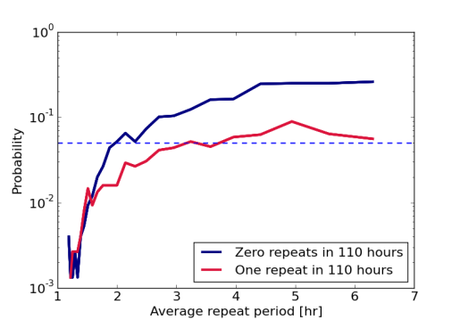
Figure 2: The probability of seeing zero (blue curve) or one (red curve) repeat burst in 110 hours of follow-up, assuming a 1/$f$ distribution. The curves are derived from a simple Monte Carlo in which a pink distribution was generated with one sample per hour, and we asked how many bursts were seen in 110 samples. Thousands of 110-hour realizations were then averaged for each repeat period, $P$. Even with an average repeat rate of once every two hours, there is still a 5$\%$ chance (indicated by the dashed line) of seeing one or fewer bursts, despite the expected value of 55.

3 Event rates and total number of sources

If FRBs were found to repeat, their statistics and the average frequency of their repetition should affect the search strategy of upcoming surveys. For instance, if it were found that FRBs repeated, on average, five times a day, then the number of unique sources would be five times smaller than the per-sky daily event rate. This means the daily rate $3.3^{+5.0}_{-2.5}\times 10^{3}$ sky^-1 estimated by Rane et al. (2015) would be produced by only $\sim$160-1600 sources. In this scenario there is no FRB in most pixels on the sky, which means one could integrate on most patches forever without seeing an event. An example of this strategy is the VLA millisecond search, in which $\sim 40\%$ of the time was spent at a single pointing, and almost three quarters of the time was spent at just three locations (Law et al., 2015). It is possible that pointing-to-pointing event rate variance contributed to their not seeing anything.

We therefore warn that deep surveys are at a disadvantage to those that sweep large regions of the sky (CHIME (Bandura, 2014), UTMOST, HIRAX) because the non-repeating scenario is unaffected; whereas shallow observations should not hurt the detection rate, no matter what their repetition. Ideally, a survey needs only to spend a few dispersion delay times on each beam before moving on.

4 Latitudinal dependence

There is now evidence that the FRB rate is nonuniform on the sky, with fewer detectable events at low Galactic latitudes (Burke & Graham-Smith, 2014). However the statistical significance of this finding may be overestimated. Petroff et al. (2014) compute the probability of the disparity between the number of bursts seen in the high- and intermediate-latitude ($|b|<15\degree$) components of the High Time Resolution Universe survey (HTRU). They calculate the probability of seeing $N=0$ in the intermediate latitude survey and $M=4$ in the high-latitude, despite having searched 88$\%$ more data in the former, and they rule out the uniform sky hypothesis with 99.5$\%$ certainty. We would point out that in general $P(N|M)$ describes a very specific outcome, and it would be more appropriate to include all outcomes equally or more unlikely. That number might also be multiplied by two, since if the survey found four intermediate-latitude FRBs and zero high-lat ones, we would ask the same question.

But a simpler approach to this problem would be analogous to a series of coin flips. If a coin were flipped four times, the probability of seeing all heads is 1/16, or 6.25$\%$. This is a factor of six higher than the analogous analysis of Petroff et al. (2014). We can test the null hypothesis that the coin is fair, and using the binomial statistic would conclude that the outcome is consistent with a fair coin at 95% confidence, differing from the conclusion of Petroff et al. (2014). In the FRB case the Universe is flipping a coin each time a new burst appears, with some bias factor due to things like different integration times. HTRU has since reported five more bursts in the high Galactic region, but using a dataset that spent $\sim$2.5 times more time at high latitudes. Below we try and quantify the likelihood of this.

If one wants to compare two statistical hypotheses, then the claims of each should be treated as true and their likelihood discrepancy should be computed. In the case of testing the abundance of FRBs at high latitudes, the sky should be partitioned into high and low regions a priori (e.g., the predefined high-latitude HTRU and its complement). The rate in both regions is then taken to be the same, and the likelihood of a given spatial distribution of observed sources can be calculated. This situation is naturally described by a biased binomial distribution with a fixed number of events. Suppose a total of $K$ FRBs are observed in a given survey. We can ask the question, what is the probability of seeing $M$ events in the high region and ($K-M$) events in the lower region? This probability can be calculated as

$$P(M|\,{K},p)=\binom{K}{M}\,p^{M}(1-p)^{K-M},$$ (2)

where $p$ is the probability that an event happens to show up in the high region. In a survey where more time is spent on one part of the sky than the other, $p=\alpha/(\alpha+1)$, where $\alpha$ is the ratio of time spent in the high-latitude region vs. the intermediate region. In the case of the HTRU survey, $K=9$ and since none were found in the low-latitude region, $M=9$. Roughly 2500 hours were spent searching the upper region and $\sim 1000$ hours were spent at $|b|<15\degree$, giving $\alpha=2.5$. Using Equation 2, this outcome is only $\sim 5\%$ unlikely.

The problem is given a quasi-Bayesian treatment by Petroff et al. (2014), which gives the following.

$$P(N|\,M)=\alpha^{N}(1+\alpha)^{-(1+M+N)}\frac{(M+N)!}{M!N!}$$ (3)

This gives a probability of $\sim$3.5$\%$, using all nine FRBs. This method is Bayesian in the sense that they marginalize over the unknown rate and calculate a likelihood, but they then calculate a confidence and do not look at a posterior.

The most obvious difference between the approach we have offered (biased coin-flip) and the quasi-Bayesian method is that we take $M+N$ to be fixed. It follows to ask whether or not we should regard the total number of FRBs as “given”? We believe the answer is yes, since this is one of the few quantities that we have actually measured, along with $M$ and $N$. What we are really trying to infer is how much larger $\mu_{\textup{high}}$ is than $\mu_{\textup{low}}$, so these rates should not be marginalized over.

To consider only the likelihood can give misleading results. For example, as more and more FRBs are detected, the likelihood of the particular observed values for $N$ and $M$ will become smaller and smaller, due to the sheer number of possible tuples $(N,M)$. To decide whether or not there is evidence for FRBs to occur with a higher probability at high latitudes, we can instead use the formalism of Bayesian model selection. This formalism does not aim to rule out a particular model, it only compares the validity of two models. For this, we formulate two specific models, Model 1 in which we assume that $p_{1}=\alpha/(1+\alpha)$ as above (i.e. uniform rate across the sky), and Model 2 in which we regard $p$ as a free parameter, equipped with a flat prior between 0 and 1. The model selection will then be based on the comparison of the posterior probabilities for the two models,

$$\frac{P(\mathrm{Model}~{}1|M,K)}{P(\mathrm{Model}~{}2|M,K)}=\frac{P(M|\mathrm{Model}~{}1,K)}{P(M|\mathrm{Model}~{}2,K)},$$ (4)

where we have assumed equal prior weights for the two models. Using the binomial likelihood, Eq. (2), and marginalizing over the unknown probability $p$ in the case of Model 2, this ratio is easily calculated to be

$$\frac{P(M|\mathrm{Model}~{}1,K)}{P(M|\mathrm{Model}~{}2,K)}=(K+1)\,\binom{K}{M}\,p_{1}^{M}\,\left(1-p_{1}\right)^{K-M}.$$ (5)

For the observations discussed above with $M=K=9$ and $\alpha=2.5$, we find a ratio of $0.48$, so there is no strong preference for either of the two models.

5 Conclusions

The search for FRBs with multiple surveys that have disparate sensitivities, frequency coverage, and survey strategy (not to mention non-publication bias) has made it difficult even to estimate a daily sky rate. That combined with the relatively low number of total FRBs observed has meant that dealing with their statistics can be non-trivial. In the case of repetition, we remind the reader that several non-cataclysmic models for FRBs are expected to repeat. In the case of supergiant pulses from pulsars, SGR radio flares, or even Galactic flare stars, it is possible that this repetition would be non-stationary and might exhibit strong correlations in time. We have shown that if the repetition had some associated flicker noise and its power spectrum were 1/$f^{\gamma}$, then one should expect the repetition rate to be higher immediately after the initial FRB detection. Therefore follow-up observations to archival discoveries that take place years or months after the first event would not provide strong upper limits. This would also mean that if no burst is found in a given beam after some integration time, then it is unlikely that one will occur in the following integration, and therefore a new pointing should be searched. In other words, shallow fast surveys would be favourable.

In Section 4 we offered a simple way of quantifying the latitudinal dependence of FRBs with a binomial distribution. This is akin to a biased coin flip, in which we ask “what is the probability of $M$ bursts being found in one region and $N$ bursts in its complement, given $\alpha$ times more time was spent in the former”. Like Rane et al. (2015) we argue that the jury is still out on the severity of the latitudinal dependence. With current data the preference for FRBs to be discovered outside of the plane seems consistent with sky-temperature effects and increased scattering, or even pure chance. Whether or not more sophisticated explanations (e.g., Macquart & Johnston 2015) are required remains to be seen. We also provided a Bayesian framework for model comparison, which can be used in the limit where large numbers of FRBs have been detected.

6 Acknowledgements

We thank NSERC for support.

References

- Bandura (2014) Bandura K. e. a., 2014, in Society of Photo-Optical Instrumentation Engineers (SPIE) Conference Series Vol. 9145 of Society of Photo-Optical Instrumentation Engineers (SPIE) Conference Series, Canadian Hydrogen Intensity Mapping Experiment (CHIME) pathfinder. p. 22
- Burke & Graham-Smith (2014) Burke B. F., Graham-Smith F., 2014, An Introduction to Radio Astronomy
- Burke-Spolaor & Bannister (2014) Burke-Spolaor S., Bannister K. W., 2014, ApJ, 792, 19
- Connor et al. (2015) Connor L., Sievers J., Pen U.-L., 2015, ArXiv e-prints
- Falcke & Rezzolla (2014) Falcke H., Rezzolla L., 2014, A&A, 562, A137
- Law et al. (2015) Law C. J., Bower G. C., Burke-Spolaor S., Butler B., Lawrence E., Lazio T. J. W., Mattmann C. A., Rupen M., Siemion A., VanderWiel S., 2015, ApJ, 807, 16
- Macquart & Johnston (2015) Macquart J.-P., Johnston S., 2015, MNRAS, 451, 3278
- Maoz et al. (2015) Maoz D., Loeb A., Shvartzvald Y., Sitek M., Engel M., Kiefer F., Kiraga M., Levi A., Mazeh T., Pawlak M., Rich R. M., Tal-Or L., Wyrzykowski L., 2015, ArXiv e-prints 1507.01002
- Mickaliger et al. (2012) Mickaliger M. B., McLaughlin M. A., Lorimer D. R., Langston G. I., Bilous A. V., Kondratiev V. I., Lyutikov M., Ransom S. M., Palliyaguru N., 2012, ApJ, 760, 64
- Milotti (2002) Milotti E., 2002, ArXiv Physics e-prints
- Mingarelli et al. (2015) Mingarelli C. M. F., Levin J., Lazio T. J. W., 2015, ApJ, 814, L20
- Mottez & Zarka (2014) Mottez F., Zarka P., 2014, A&A, 569, A86
- Pen & Connor (2015) Pen U.-L., Connor L., 2015, ApJ, 807, 179
- Petroff et al. (2015) Petroff E., Bailes M., Barr E. D., Barsdell B. R., Bhat N. D. R., Bian F., Burke-Spolaor S., Caleb M., Champion D., Chandra P., Da Costa 2015, MNRAS, 447, 246
- Petroff et al. (2015) Petroff E., Johnston S., Keane E. F., van Straten W., Bailes M., Barr E. D., Barsdell B. R., Burke-Spolaor S., Caleb M., Champion D. J., Flynn C., Jameson A., Kramer M., Ng C., Possenti A., Stappers B. W., 2015, MNRAS, 454, 457
- Petroff et al. (2014) Petroff E., van Straten W., Johnston S., Bailes M., Barr E. D., Bates S. D., Bhat N. D. R., Burgay M., Burke-Spolaor S., Champion 2014, ApJ, 789, L26
- Popov & Postnov (2007) Popov S. B., Postnov K. A., 2007, ArXiv e-prints
- Press (1978) Press W. H., 1978, Comments on Astrophysics, 7, 103
- Rane et al. (2015) Rane A., Lorimer D. R., Bates S. D., McMann N., McLaughlin M. A., Rajwade K., 2015, ArXiv e-prints 1505.00834
- Thornton (2013) Thornton D. e. a., 2013, Science, 341, 53
- Totani (2013) Totani T., 2013, PASJ, 65, L12
- Voss & Clarke (1975) Voss R. F., Clarke J., 1975, Nat, 258, 317