Hawking Radiation of Mass Generating Particles From Dyonic Reissner Nordström Black Hole

Abstract

The Hawking radiation is considered as a quantum tunneling process, which can be studied in the framework of the Hamilton-Jacobi method. In this study, we present the wave equation for a mass generating massive and charged scalar particle (boson). In sequel, we analyze the quantum tunneling of these bosons from a generic 4-dimensional spherically symmetric black hole. We apply the Hamilton-Jacobi formalism to derive the radial integral solution for the classically forbidden action which leads to the tunneling probability. To support our arguments, we take the dyonic Reissner-Nordström black hole as a test background. Comparing the tunneling probability obtained with the Boltzmann formula, we succeed to read the standard Hawking temperature of the dyonic Reissner-Nordström black hole.

I Introduction

In 1975, Stephen Hawking (one of the world’s most famous physicists) made a shocking claim that when Quantum Mechanics is allied with the General Relativity, black holes (BHs) become to glow with Hawking radiation (HR) Haw1 ; Haw2 ; Haw3 ; Haw4 . This emission consists of all sorts of massless/massive particles with different spins: spin$-0,1/2,1$…. Hawking’s prodigious calculations are based on a scenario that ubiquitous virtual particle pairs are continually being created near the event horizon of the BH due to the vacuum fluctuations. Principally, these particles are created as a particle-antiparticle pair and immediately after they quickly annihilate each other. However, it is always possible that the one with negative energy (in order to conserve the total energy) falls into the BH while the other possessing the positive energy escapes to spatial energy as HR. Today, HR is also called the Bekenstein-Hawking radiation in virtue of Bekenstein’s remarkable contributions bek1 ; bek2 ; bek3 ; bek4 to this phenomenon.

Since 1975, the studies concerning HR have been carrying on. Up to the present times, many different methods for the HR are proposed (the reader may refer to gib1 ; gib2 ; vanzo ; umetso ; kraus1 ; kraus2 and references therein). Among them, the most fascinating quantum tunneling methods are Parikh and Wilczek’s null-geodesic method wilczek1 ; wilczek2 ; wilczek3 and the semiclassical methods of Hamilton-Jacobi ang ; sri1 ; sri2 ; man0 and Damour-Ruffini ruf . On the other hand, the HR of photons, scalar particles, massive vector bosons, and fermions from various BHs have been gained much attention in recent years (see for example sakhal ; sak1 ; Ma ; sak2 ; Ji ; sak3 ; sak4 ; ao1 ; mann1 ; mann2 ; mann3 ; xiang ; kruglov1 ; kruglov2 ; ao2 ; aoo2 ; ao3 ; ao4 ; ao6 ; frasca ; valt ; rocha ; gos ; sing ; zhi ; yangg ). Furthermore, the information loss paradox loss1 ; loss2 ; loss3 in the HR is one of the great puzzles for the physics community. Some theorists bring forward an idea to retrieve the information from the BH encoded in the HR haw15 ; hooft ; hooft1 ; dvali ; lochan ; stoica ; kraus ; louko ; rman ; calmet ; perez ; papa ; shi ; marolf ; malda . However, this mystery have not been solved literally.

In the 1970s, particle physicists realized that there are very close ties between two of the four fundamental forces force ; sm1 ; sm2 ; sm3 ; sm4 ; sm5 ; sm6 – the weak force and the electromagnetic force which is single underlying force known as the electroweak force. The basic equations of the unified theory correctly describe the relationship between the electroweak force and its associated force-carrying particles [photons and the massive vector bosons ($W^{\pm}$ and $Z$)], except for a major glitch: all of these particles emerge without a mass! Although this is true for the photon, we know that the $W^{\pm}$ and $Z$ bosons must have mass, nearly hundred times that of a proton. The problem of spontaneously broken gauge theories in curved spacetime is well known in literature barroso ; tro ; rand ; arkani ; witt ; dad0 ; dad1 . So far, the Higgs mechanism sm4 ; sm5 is the experimentally confirmed mechanism to solve the generation of mass problem in particle physics, which satisfies both the unitarity and the renormalization of the theory.

In this paper, we make a brief review for the derivation of the wave equation for the mass generating (massive and charged) scalar particles. Applying the resulting equation obtained to the general 4-dimensional static and spherically symmetric metric, we obtain the general radial integral solution for the action of Hamilton-Jacobi method. As a test bed we consider the dyonic Reissner-Nordström BH (DRNBH) dy and compute its quantum tunneling rate by using the latter radial integral solution of the action. Finally, we show in detail how one recovers the original HR of the DRNBH from the quantum tunneling of the mass generating particles.

The paper is organized as follows. In Sec. II, we introduce the wave equation of a massive and charged mass generating scalar particle in a curved spacetime. Section III is devoted to the computations of the quantum tunneling of the mass generating scalar particles from the DRNBH. While doing this, we are attentive to make our calculations with generic as much as possible. We draw our conclusions in Sec. IV.

II Wave Equation of Mass Generating Particles

In this section, we represent an expression for the wave equation of the mass generating particles. Their associated scalar fields are non-minimally coupled to the gravity. The main idea underlying this mass generation mechanism is resplendently introduced in many textbooks (see for instance qft1 ; la ).

For brevity, we initially use units $G_{N}=c=\hbar=1$. One may write down the action of the interaction of the scalar fields with gravity barroso as follows

$$S=\int d^{4}x\sqrt{-g}\left[\frac{\Re}{16\pi}-\xi\phi^{{\dagger}}\phi\Re+(D_{\mu}\phi)^{{\dagger}}D^{\mu}\phi-V(\phi)-\frac{1}{4}F_{\mu\nu}F^{\mu\nu}\right],$$ (1)

where $\Re$ stands for the scalar curvature and $F_{\mu\nu}=\nabla_{\mu}A_{\nu}-\nabla_{\nu}A_{\mu}$ is the Maxwell field strength with the spin-1 gauge field $A_{\nu}$ (electromagnetic vector potential). $\xi$ denotes the dimensionless coupling constant which governs the non-minimal interaction of the scalar field $\phi$ foot1 with gravity. In other words, the minimally coupled scalar fields correspond to $\xi=0$. It is worth noting that this coupling constant $\xi$ can also be used to stabilize the vacuum expectation value $y^{2}=\frac{v^{2}}{2}=\left\langle\phi^{{\dagger}}\phi\right\rangle$ near the event horizon of a BH dad1 . The gauge-covariant derivative is given by

$$D_{\mu}=\partial_{\mu}-ieA_{\mu},$$ (2)

where $e$ is the coupling constant (i.e. the Planck charge) of the electromagnetic vector potential $A_{\mu}$. The variation of the action (1) with respect to the metric tensor $g_{\mu\nu}$ leads to the Einstein equations of motion as follows

$$\Re_{\mu\nu}-\frac{1}{2}\Re g_{\mu\nu}=-8\pi T_{\mu\nu},$$ (3)

where $T_{\mu\nu}$ is the energy-momentum tensor. Its overlong expression can be seen in the study of Moniz et al barroso . Significantly, when one applies the variation to the action (1) with respect to $\phi^{{\dagger}}$, the following wave equation is obtained

$$\frac{1}{\sqrt{-g}}\left(\partial_{\mu}-ieA_{\mu}\right)\left[\sqrt{-g}g^{\mu\nu}\left(\partial_{\nu}-ieA_{\nu}\right)\phi\right]+\xi\Re\phi+\partial_{\phi^{{\dagger}}}V=0.$$ (4)

The mass generating potential was also defined in barroso as follows

$$V(\phi)=B+\widetilde{m}^{2}\phi^{{\dagger}}\phi+\lambda(\phi^{{\dagger}}\phi)^{2},$$ (5)

where $B$ is an arbitrary constant and the coupling constant $\lambda$ is dimensionless in 4-dimensional spacetime. Without loss of generality, it is assumed that $\lambda$ has a positive definite value. As clearly stated in barroso , the vacuum expectation value must satisfy the condition of $y^{2}\neq 0$, which requires that $V(\phi)$ must have a minimum at $\phi\neq 0$. To obtain the bounded solution for the Hamiltonian, $\widetilde{m}^{2}$ must be negative since $\lambda$ is positive. Due to this reason, we shift $\widetilde{m}^{2}\rightarrow-m^{2}$. Hence, using Eq. (5), we have

$$\partial_{\phi^{{\dagger}}}V=\left[-m^{2}+2\lambda(\phi^{{\dagger}}\phi)\right]\phi.$$ (6)

After assigning the reduced Planck constant back to its original value $\hslash$, Eq. (4) can be rewritten as

$$\frac{1}{\sqrt{-g}}\left(\partial_{\mu}-i\frac{e}{\hslash}A_{\mu}\right)\left[\sqrt{-g}g^{\mu\nu}\left(\partial_{\nu}-i\frac{e}{\hslash}A_{\nu}\right)\phi\right]+\frac{1}{\hslash^{2}}\left[\xi\Re-m^{2}+2\lambda(\phi^{{\dagger}}\phi)\right]\phi=0.$$ (7)

which is the wave equation of the mass generating particles with mass $m$ and charge $e$ in a curved spacetime. It is also important to know that whenever the scalar field $\phi$ is used for a Nambu–Goldstone boson in the gauge theory of spontaneous symmetry breaking, $\xi$ is zero volo . On the other hand, if the scalar field $\phi$ represents a composite particle, then the value of $\xi$ is fixed by the dynamics of its components. In particular, $\xi=1/6$ in the large $N$ approximation to the Nambu-Jona-Lasinio model hill . Moreover, in the standard model, the Higgs fields possess the values of $\xi$ within the range of $\xi\leq 0$ and $\xi\geq 1/6$ hoso .

III Quantum Tunneling of Mass Generating Particles from DRNBH

The line-element for the 4-dimensional generic static (spherically symmetric) BH metric is given by

$$ds^{2}=-Fdt^{2}+G^{-1}dr^{2}+R\left(d\theta^{2}+\sin^{2}\theta d\varphi^{2}\right),$$ (8)

where the metric functions $\left(F,G,R\right)$ are only the function of $r$. Any horizon $r_{h}$ should satisfy the condition of $G(r_{h})=0$ and $r_{h}$ is, in general, a function of the mass and charge of the BH. The Hawking temperature of a BH described by the metric (8) is given by fer

$$T_{H}=\frac{1}{4\pi}\left.\left|\frac{dg_{tt}}{dr}\right|\sqrt{-g^{tt}g^{rr}}\right|_{r=r_{h}}=\frac{F^{\prime}\left(r_{h}\right)}{4\pi\sqrt{B\left(r_{h}\right)}},$$ (9)

where $B=\frac{F}{G}$ and the prime over a quantity denotes the derivative with respect to $r$. Furthermore, the Ricci scalar wald for the metric (8) can be found as

$$\Re =\frac{1}{2F^{2}R^{2}}(-G^{\prime}F^{\prime}FR^{2}-2F^{\prime\prime}FGR^{2}+F^{{}^{\prime}2}GR^{2}-$$

$$2RGF^{\prime}R^{\prime}F+R^{\prime 2}F^{2}G-4R^{\prime\prime}F^{2}GR-2G^{\prime}R^{\prime}F^{2}R+4F^{2}R).$$ (10)

In order to study the quantum tunneling of the mass generating particles from the generic BH (8), we use the WKB approximation and assume an ansatz for the scalar field $\phi$ as follows

$$\phi=c\exp\left(\frac{i}{\hbar}I(t,r,\theta,\varphi)\right),$$ (11)

where $c$ is the amplitude of the wave and $I$ stands for the classically forbidden action of the trajectory. Metric (8) admits two Killing vectors $<$ $\partial_{t}$, $\partial_{\varphi}$ $>$, which show the existence of the symmetries. Therefore, one can assume a solution for the action as

$$I=-Et+W(r)+j(\theta,\varphi)+C,$$ (12)

where $E$ denotes energy, $W(r)$ and $j(\theta,\varphi)$ are radial and angular functions, respectively. In Eq. (12) $C$ is a complex constant.

Since $A_{\nu}$ represents the electromagnetic vector potential, for a dyonic BH with electric and magnetic components one should have $A_{\nu}=\left[A_{0}(r),0,0,A_{1}(\theta)\right]$. Under the guidance of the Hamilton-Jacobi method ang , we first insert Eqs. [11-13] in Eq. (7) and then consider the terms with the leading order of $\hbar$. Thus, we obtain the following lenghty expression

$$\sin^{2}\theta\{\left[(-G^{\prime}F^{\prime}-2F^{\prime\prime}G)F+F^{\prime 2}G\right]R^{2}-2\left[\left(G^{\prime}R^{\prime}-2+2GR^{\prime\prime}\right)F+GF^{\prime}R^{\prime}\right]FR+R^{\prime}F^{2}G\}\xi$$

$$-2FR\left\{\left[(-m^{2}-2\,\lambda c^{2}-GW^{\prime 2})R-{j_{\theta}}^{2}\right]\mathrm{\sin}^{\mathrm{2}}\theta-(eA_{1}-{j_{\varphi}})^{2})F+R\mathrm{\sin}^{\mathrm{2}}\theta E_{net}^{2}\right\}=0,$$ (13)

where ${j_{\theta}}=\frac{\partial j}{\partial\theta}$, ${j_{\varphi}}=\frac{\partial j}{\partial\varphi}$, and $E_{net}=E+eA_{0}$. From Eq. (13), we derive an integral solution for $W(r)$ as follows

$$W_{\pm}=\pm\int\frac{1}{\sqrt{FG}}\left[\left(n_{1}F+n_{2}\right)\xi G+\frac{F}{R}n_{3}+E_{net}^{2}\right]^{\frac{1}{2}}dr,$$ (14)

where

$$n_{1}={\frac{2R^{\prime\prime}}{R}}+{\frac{G^{\prime}R^{\prime}-2}{GR}}-{\frac{1}{2}}\left({\frac{R^{\prime}}{R}}\right)^{2},$$ (15)

$$n_{2}=\frac{F^{\prime 2}}{2F}-\frac{F^{\prime}R^{\prime}}{R}-\frac{1}{2}\frac{G^{\prime}F^{\prime}}{G}-F^{\prime\prime},$$ (16)

$$n_{3}=(-2c^{2}\lambda-m^{2})R-{j_{\theta}}^{2}-\frac{(eA_{1}-{j_{\varphi}})^{2}}{\mathrm{\sin}^{\mathrm{2}}\theta}.$$ (17)

Since $G(r_{h_{+}})=0$, the near horizon form of Eq. (14) becomes

$$W_{\pm}\approx\pm\int\sqrt{\frac{E_{net}^{2}R+Fn_{3}}{RFG}}dr.$$ (18)

which is essential expression for computing the quantum tunneling rate. Now, we test the above result obtained via the DRNBH geometry dy whose the metric functions and electromagnetic vector potential components are given by

$$F=G=\frac{\left(r-r_{h_{+}}\right)\left(r-rh_{{}_{-}}\right)}{r^{2}},$$ (19)

$$R=r^{2},$$ (20)

$$A_{0}=-\frac{Q}{r},\text{ \ \ }A_{1}=P\cos\theta.$$ (21)

where the physical quantities $Q$ and $P$ denote the DRNBH’s characteristic parameters: $Q$ is the electric charge and $P$ is the magnetic charge. The outer or event ($r_{h+}$) and inner ($r_{h-}$) horizons of the DRNBH are given by

$$r_{h_{\pm}}=M\pm\sqrt{M^{2}-\Theta^{2}},$$ (22)

where $\Theta^{2}=Q^{2}+P^{2}$. In Eq. (22) the parameter $M$ represents the mass of the DRNBH. Since $F=G,$ consequently $Fn_{3}\rightarrow 0$ around the event horizon. Here, one can immediately criticize why the $n_{3}$ parameter including the particle’s mass $m$ quickly drops out of the considerations. However, one can experience from the previous studies vanzo that the non-differential terms coupled to the wave function $\phi$ (for example, in Eq. (7), it corresponds to $\frac{1}{\hslash^{2}}\left[\xi\Re-m^{2}+2\lambda(\phi^{{\dagger}}\phi)\right]\phi$ ) apart from the operator term acting on $\phi$ (like the Laplacian operator: $\square\phi$) always looses its effiency near the horizon. That is why, for instance, the HR is independent from the particle’s mass ex1 ; ex2 . Thus, Eq. (18) reduces to

$$W_{\pm}\approx\pm\int\frac{E_{net}}{F}dr.$$ (23)

Meanwhile, we now have $E_{net}=E-\frac{eQ}{r_{h_{+}}}$. It is obvious that the above integrand possesses a simple pole at the event horizon. To evaluate integral (23), we first expand the metric function $F$ as follows

$$F(r)=F^{\prime}(r_{h_{+}})(r-r_{h_{+}})+\Game(r-r_{h_{+}})^{2}.$$ (24)

Substituting the above expression into Eq. (23) and choosing the contour as a half loop going around this pole from left to right, one obtains

$$W_{\pm}=\pm i\pi\frac{E_{net}}{F^{\prime}\left(r_{h_{+}}\right)}.$$ (25)

Thus, the imaginary part of the action (12) becomes

$$\operatorname{Im}I_{\pm}=ImC\pm\pi\frac{E_{net}}{F^{\prime}\left(r_{h_{+}}\right)}.$$ (26)

Thence, we compute the probabilities of ingoing and outgoing particles tunneling the DRNBH horizon as

$$P_{in}=\exp(-2ImI_{-})=\exp\left(-2ImC+2\pi\frac{E_{net}}{F^{\prime}\left(r_{h_{+}}\right)}\right),$$ (27)

$$P_{out}=\exp(-2ImI_{+})=\exp\left(-2ImC-2\pi\frac{E_{net}}{F^{\prime}\left(r_{h_{+}}\right)}\right).$$ (28)

Classically, having a BH is conditional on the no-reflection for the ingoing waves, which meants full absorption: $P_{in}=1$. This is possible simply by setting $ImC=\pi\frac{E_{net}}{F^{\prime}\left(r_{h_{+}}\right)}$ (for similar and recent works, the reader is referred to con1 ; con2 ; con3 and references therein) which results in

$$P_{out}=\exp\left(-4\pi\frac{E_{net}}{F^{\prime}\left(r_{h_{+}}\right)}\right).$$ (29)

Consequently, we read the quantum tunneling rate for the DRNBH as

$$\Gamma=\frac{P_{out}}{P_{in}}=\exp\left(-4\pi\frac{E_{net}}{F^{\prime}\left(r_{h_{+}}\right)}\right).$$ (30)

Employing the Boltzmann formula $\Gamma=\exp(-E_{net}/T)$ bolt , the surface temperature of the DRNBH can be computed as

$$T=\frac{F^{\prime}\left(r_{h_{+}}\right)}{4\pi}=\frac{r_{h_{+}}-r_{h_{-}}}{r_{h_{+}}^{2}}=\frac{\sqrt{M^{2}-\Theta^{2}}}{2\pi\left(M+\sqrt{M^{2}-\Theta^{2}}\right)^{2}},$$ (31)

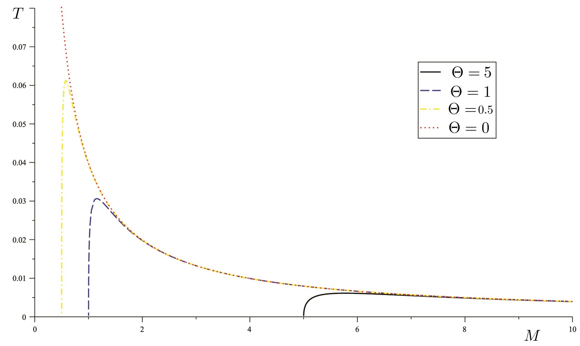
which is exactly equal to the standard Hawking temperature of the DRNBH dy . Temperature versus mass plotting is depicted in Fig. (1) for $M\geq\Theta$. As it can be seen from Fig. (1), the locations of the peaks on the $M$-axis (which are very close to their associated starting mass value $M_{initial}=\Theta$: the extreme BH case, $T=0$) shift towards right with increasing $M$-value, however the peak values decrease when $M_{initial}$ gets bigger numbers. Moreover, while $M\rightarrow\infty,$ all the curves of the temperatures rapidly reach to the curve of the Schwarzschild ($\Theta=0$) BH’s Hawking temperature, which goes to zero with increasing $M$-value.

Figure 1: Plots of the temperature $T$ versus DRNBH mass $M$. The plots are governed by Eq. (31). The starting masses are governed by $M_{initial}=\Theta$.

IV Conclusion

In this paper, we firstly reviewed the derivation of the wave equation for the mass generating scalar particles in the concept of the spontaneous symmetry breaking theory. To this end, we introduced an action involving a non-minimal scalar field coupled to the gravity. By using the Hamilton-Jacobi method with a suitable WKB ansatz, the quantum tunneling of the mass generating bosons from a generic static BH is thoroughly studied. We then obtained the general integral solution for the radial function (14) for the Hamilton-Jacobi action $I$. DRNBH geometry whose the metric functions satisfy the equality $F=G$ is considered as a test background for our computations. It is seen that scalar particle mass $m$, the non-minimal coupling constant $\xi$, and the potential constant $\lambda$ are not decisive for the quantum tunneling rate, however the charge $e$ is. In the semiclassical framework, we computed the probabilities of the ingoing and outgoing particles to get the quantum tunneling rate for the DRNBH. Finally, we managed to read the standard Hawking temperature of the DRNBH via the Boltzmann formula of the tunneling rate.

In future work, we plan to extend our analysis to a BH (might be a spherically non-symmetric) having $F$, which does not vanish at the event horizon: $F(r_{h})\neq 0$. Because in such a case Eq. (18) may yield such $W_{\pm}$ values (having now the potential constant term $\lambda$ ) that the quantum tunneling rate can deviate from its pure thermal character foot2 and give contribution to the information loss problem loss3 . We also aim to extend our analysis to the dynamic, rotating and higher/lower dimensional BHs. In this way, we will analyze the HR of the mass generating particles from various BHs.

References

- (1) S. W. Hawking, Phys. Rev. Lett. 26, 1344 (1971).
- (2) S. W. Hawking, Nature 248, 30 (1974).
- (3) S. W. Hawking, Commun. Math. Phys. 43, 199 (1975); erratum-ibid, 46, 206 (1976).
- (4) S. W. Hawking, Phys. Rev. D 13, 191 (1976).
- (5) J. D. Bekenstein, Lett. Nuovo Cimento 4, 737, (1972).
- (6) J. D. Bekenstein, Phys. Rev. D 7, 2333, (1973).
- (7) J. D. Bekenstein, Phys. Rev. D 9, 3292 (1974).
- (8) J. D. Bekenstein, Phys. Rev. D 12, 3077 (1975).
- (9) G. W. Gibbons and S. W. Hawking, Phys. Rev. D 15, 2738 (1977).
- (10) G. W. Gibbons and S. W. Hawking, Phys. Rev. D 15, 2752 (1977).
- (11) L. Vanzo, G. Acquaviva, and R. Di Criscienzo, Classical Quant. Grav. 28, 18 (2011).
- (12) K. Umetsu, Phys. Lett. B 692, 61 (2010).
- (13) P. Kraus and F. Wilczek, Mod. Phys. Lett. A 9, 3713 (1994).
- (14) P. Kraus and F. Wilczek, Nucl. Phys. B 437, 231 (1995).
- (15) M. K. Parikh and F. Wilczek, Phys. Rev. Lett. 85, 5042 (2000).
- (16) M. K. Parikh, Phys. Lett. B 546, 189 (2002).
- (17) M. K. Parikh, Int. J. Mod. Phys. D 13, 2351 (2004).
- (18) M. Angheben, M. Nadalini, L. Vanzo, and S. Zerbini, J. High Energy Phys. 05, 014 (2005).
- (19) K. Srinivasan and T. Padmanabhan, Phys. Rev. D 60, 024007 (1999).
- (20) S. Shankaranarayanan, K. Srinivasan, and T. Padmanabhan, Mod. Phys. Lett. 16, 571 (2001).
- (21) R. Kerner and R. B. Mann, Phys. Rev. D 73, 104010 (2006).
- (22) T. Damour and R. Ruffini, Phys. Rev. D 14, 332 (1976).
- (23) I. Sakalli, M. Halilsoy, and H. Pasaoglu, Astrophys. Space Sci. 340, 155 (2012).
- (24) I. Sakalli, Int. J. Theor. Phys. 50 , 2426 (2011).
- (25) S. H. Mazharimousavi, M. Halilsoy, I. Sakalli, and O. Gurtug, Classical Quant. Grav. 27, 105005 (2010).
- (26) I. Sakalli, A. Ovgun, and S. F. Mirekhtiary, Int. J. Geom. Methods Mod. Phys. 11, 1450074 (2014).
- (27) Q. Q. Jiang, Classical Quant. Grav. 24, 4391 (2007).
- (28) I. Sakalli and A. Ovgun, EPL 110, 10008 (2015).
- (29) I. Sakalli and A. Ovgun, Eur. Phys. J. Plus 130, 110 (2015).
- (30) I. Sakalli and A. Ovgun, Astrophys. Space Sci. 359, 32 (2015).
- (31) R. Kerner and R. B. Mann, Classical Quant. Grav. 25, 095014 (2008).
- (32) R. Kerner and R. B. Mann, Phys. Lett. B 665, 277 (2008).
- (33) A. Yale and R. B. Mann, Phys. Lett. B 673, 168 (2009).
- (34) X. Q. Li and G. R. Chen, Phys. Lett. B 751, 34 (2015).
- (35) S. I. Kruglov, Mod. Phys. Lett. A 29, 1450203 (2014).
- (36) S. I. Kruglov, Int. J. Mod. Phys. A 29, 1450118 (2014).
- (37) A. Ovgun and K. Jusufi, Eur. Phys. J. Plus 131, 177 (2016).
- (38) K. Jusufi and A. Ovgun, Astrophys. Space Sci. 361, 207 (2016).
- (39) I. Sakalli and A. Ovgun, J. Exp. Theor. Phys. 121, 404 (2015).
- (40) I. Sakalli and A. Ovgun, Gen. Relativ. Gravit. 48, 1 (2016).
- (41) A. Ovgun, Int. J. Theor. Phys. 55, 2919 (2016).
- (42) M. Frasca, arXiv:1412.1955.
- (43) P. Valtancoli, Ann. Phys-New York 362, 363 (2015).
- (44) R. T. Cavalcanti and R. da Rocha, Adv. High Energy Phys. 2016, 4681902 (2016).
- (45) G. Goswamia, S. Mohantya, Phys. Lett. B 751, 113 (2015) .
- (46) T. Ibungochouba Singh, I. Ablu Meitei, K. Yugindro Singh, Astrophys Space Sci 361, 103 (2016) .
- (47) Z. K. Xie, J. Astrophys. Astr. 35, 553 (2014).
- (48) X. Yang, Y. Zhang, W. Liu, J., Astrophys. Astr. 35, 559 (2014).
- (49) S. B. Giddings, Phys. Rev. D 49, 4078 (1994).
- (50) M. Varadarajan, J. Phys. Conf. Ser. 140, 012007 (2008).
- (51) S. W. Hawking, arXiv:1509.01147.
- (52) S. W. Hawking, M. J. Perry, and A. Strominger, arXiv:1601.00921.
- (53) G. Hooft, Nucl. Phys. B 43, 1 (1995).
- (54) G. Hooft, Int. J. Mod. Phys. A 11, 4623 (1996).
- (55) G. Dvali, arXiv:1509.04645.
- (56) K. Lochan and T. Padmanabhan, arXiv:1507.06402, to be appeared in PRL.
- (57) O. C. Stoica, J. Phys.: Conf. Ser. 626, 012028 (2015).
- (58) P. Kraus and S. D. Mathur, Int. J. Mod. Phys. D 24, 543003 (2015).
- (59) E. Martin-Martinez and J. Louko, Phys. Rev. Lett. 115, 031301 (2015).
- (60) R. B. Mann, Fund. Theor. 178, 71 (2015).
- (61) X. Calmet, Classical Quant. Grav. 32, 045007 (2015).
- (62) A. Perez, Classical Quant. Grav. 32, 084001 (2015).
- (63) K. Papadodimas and S. Raju, Phys. Rev. Lett. 112, 051301 (2014).
- (64) S. B. Giddings and Y. Shi, Phys. Rev. D 89, 124032 (2014).
- (65) A. Almheiri, D. Marolf, and J. Polchinski, J. High Energy Phys. 1302, 062 (2013).
- (66) J. Maldacena and L. Susskind, Fortsch. Phys. 61, 781 (2013).
- (67) P. Davies, The Forces of Nature (Cambridge Univ. Press, New York, 1986).
- (68) S. L. Glashow, Nucl. Phys. 22, 579 (1961).
- (69) S. Weinberg, Phys. Rev. Lett. 19, 1264 (1967).
- (70) A. Salam, “Elementary Particle Physics: Relativistic Groups and Analyticity,” In: N. Svartholm, Ed., Eighth Nobel Symposium, Almquvist and Wiksell, Stockholm, (1968).
- (71) F. Englert and R. Brout, Phys. Rev. Lett. 13, 321 (1964).
- (72) P. W. Higgs, Phys. Rev. Lett. 13, 508 (1964).
- (73) G. S. Guralnik, C. R. Hagen, and T. W. B. Kibble, Phys. Rev. Lett. 13, 585 (1964).
- (74) P. Moniz, P. Crawford, and A. Barroso, Class. Quantum Grav. 7, L143 (1990).
- (75) S. Troitsky, Phys. Usp. 55, 72 (2012).
- (76) L. Randall and R. Sundrum, Phys. Rev. Lett. 83, 3370 (1999).
- (77) N. Arkani-Hamed, S. Dimopoulos, and G. R. Dvali, Phys.Lett. B 429, 263 (1998).
- (78) E. Witten, Nucl. Phys. B 188, 513 (1981).
- (79) D. A. Demir, Phys. Rev. D 60, 055006 (1999).
- (80) D. A. Demir, Phys. Lett. B. 733, 237 (2014).
- (81) C. M. Chen, Y. M. Huang, J. R. Sun, M. F.Wu, and S. J. Zou, Phys. Rev. D 82, 066003 (2010).
- (82) M. E. Peskin and D. V. Schroeder, An Introduction to Quantum Field Theory (Westview Press, USA, 1995).
- (83) P. Langacker, The Standard Model and Beyond (CRC Press, New Jersey, 2009).
- (84) denotes the complex conjugate of
- (85) M. B. Voloshin and A. D. Dolgov, Sov. J. Nucl. Phys. 35, 120 (1982).
- (86) C.T. Hill and D.S. Salopek, Ann. Phys-New York 213, 21 (1992).
- (87) Y. Hosotani, Phys. Rev. D 32, 1949 (1985).
- (88) S. Fernando, Gen. Rel. Grav. 37, 461 (2005).
- (89) R. M. Wald, General Relativity (The University of Chicago Press, Chicago and London, 1984).
- (90) M. Liu, J. Lu, Y. Xu, J. Lu, Y. Wu, and R. Wang, Phys. Rev. D 87, 024043 (2013).
- (91) G. Jannes, P. Maissa,T. G. Philbin, and G. Rousseaux, Phys. Rev. D 83, 104028 (2011).
- (92) H. Gohar and K. Saifullah, Astroparticle Physics 48, 82 (2013).
- (93) F. Darabi, K. Atazadeh, and A. Rezaei-Aghdam, Eur. Phys. J. C 74, 2967 (2014).
- (94) I. Sakalli and H. Gursel, Eur. Phys. J. C 76, 318 (2016).
- (95) G. Ryskin, Phys. Lett. B 734, 394 (2014).
- (96) Thermal radiations do not carry information, see for example wilczek1 .