Schwinger-Dyson approach and its application to generate a light composite scalar
Abstract
We discuss the possibility of generating a light composite scalar boson, in a scenario that we may generically call Technicolor, or in any variation of a strongly interacting theory, where by light we mean a scalar composite mass about one order of magnitude below the characteristic scale of the strong theory. Instead of most of the studies about a composite Higgs boson, which are based on effective Lagrangians, we consider this problem in the framework of non-perturbative solutions of the fermionic Schwinger-Dyson and Bethe-Salpeter equations. We study a range of mechanisms proposed during the recent years to form such light composite boson, and verify that such possibility seems to be necessarily associated to a fermionic self-energy that decreases slowly with the momentum.
pacs:
11.15.Tk, 12.60.Nz, 12.60.FrI Introduction
The GeV new resonance discovered at the LHC LHC1 ; LHC2 has many of the characteristics expected for the Standard Model (SM) Higgs boson. If this particle is a composite or an elementary scalar boson is still an open question that probably will be answered at LHC13 run. The possibility that a light composite state could be discovered at the LHC, in a scenario that we may generically call Technicolor, or in any variation of a strongly interacting theory has been extensively discussed in the literature sannino .
The chiral and gauge symmetry breaking in quantum field theories can be promoted by fundamental scalar bosons through the Higgs boson mechanism. However the main ideas about symmetry breaking and spontaneous generation of fermion and gauge boson masses in field theory were based on the superconductivity theory. Nambu and Jona-Lasinio proposed one of the first field theoretical models based on the ideas of superconductivity, where all the most important aspects of symmetry breaking and mass generation, as known nowadays, were explored at length nl . The model of Ref.nl contains only fermions possessing invariance under chiral symmetry, although this invariance is not respected by the vacuum of the theory and the fermions acquire a dynamically generated mass (). As a consequence of the chiral symmetry breaking by the vacuum the analysis of the Bethe-Salpeter equation (BSE) shows the presence of Goldstone bosons. These bosons, when the theory is assumed to be the effective theory of strongly interacting hadrons, are associated to the pions, which are not true Goldstone bosons when the constituent fermions have a small bare mass. Besides these aspects Nambu and Jona-Lasinio also verified that the theory presents a scalar bound state (the sigma meson).
In Quantum Chromodynamics (QCD) the same mechanism is observed, where the quarks acquire a dynamically generated mass (). This dynamical mass is usually expected to appear as a solution of the Schwinger-Dyson equation (SDE) for the fermion propagator when the coupling constant is above a certain critical value. The condition that implies a dynamical mass for quarks breaking the chiral symmetry is the same one that generates a bound-state massless pion. This happens because the quark propagator SDE is formally the same equation binding a quark and antiquark into the massless pseudoscalar state at zero momentum transfer (the pion). As shown by Delbourgo and Scadron scadron1 , the same similarity of equations happens for the scalar p-wave state of the BSE, indicating the presence of a bound state with mass and this scalar meson is the elusive sigma meson polosa1 ; polosa2 ; polosa3 , that is assumed to be the Higgs boson of QCD.
Inspired in QCD, Technicolor was a theory invented to provide a natural and consistent quantum-field theoretic description of electroweak (EW) symmetry breaking, without elementary scalar fields. A possibility raised a few years ago is to have a Higgs arising as a composite pseudo-Goldstone boson (PGB) from the strongly interacting sector, where in this case the Higgs mass is protected by an approximate global symmetry and is only generated via quantum effects, models based on this approach are usually called composite Higgs modelsbella . As pointed out in Refs.bella ; lane2 , composite Higgs models require a degree of fine-tuning of parameters and most of the studies about a composite Higgs boson are based on effective Lagrangians bella . The approach that we will discuss here is not based on effective Lagrangians or operators, but on the dynamics of the theory, i.e. on the non-perturbative solutions of the Schwinger-Dyson and Bethe-Salpeter equations. The freedom appearing on the coefficients of the many possible operators that can be introduced into an effective Lagrangian in order to describe the SM scalar boson sector, is traded now by the self-energies of the new fermions that form the composite scalar boson. Assuming that the underlying theory is a non-Abelian gauge theory, we will verify that the restriction imposed on the theory parameters by the existence of a light scalar composite are quite tight, and the construction of a realistic “Technicolor” model may indeed be a very precise engineering problem.
In a very recent paper, ATLAS and CMS Collaborations ATLAS-CMS , based on their combined data samples presented an improved precision value for . The improved knowledge of yields more precise predictions for the Higgs couplings and until now the coupling strengths to SM particles are consistent within the uncertainties expected for the SM Higgs boson. Probably in a realistic composite scalar model the fermionic couplings will involve an ETC group(or GUT) with a delicate vacuum alignment between two type of composite scalar bosons and , where one of the composites resemble a fundamental scalar and the fermionic masses are not generated as usual, by different ETC mass scales, but by a different mechanism. In the Ref.us2 we considered a TC model with a horizontal symmetry where the top quark (or the third fermionic generation) obtain its mass associated to a large ETC scale, and in this case only the composite boson is coupled to the third fermionic generation, with a coupling resembling the one of a fundamental scalar boson, although the aspects of generating the SM fermionic mass spectrum will not be touched here. We just commented this in order to remember that the generation of a light scalar composite is only part of the problem if we desire the full SM dynamical symmetry breaking, where the generation of the fermionic mass spectra is another enormous step in this direction, and, probably, the larger part of the problem.
Our intent in this work is not to advocate that the GeV scalar boson is a composite one, but to discuss how a scalar composite boson can be generated with a mass lighter than the characteristic scale of the strongly interacting theory. Of course, we will resort to our knowledge about QCD, where the lightest scalar boson has a mass about twice the characteristic scale , as well as we will make analogy to the SM where the scalar responsible for the gauge symmetry breaking has a mass about one order of magnitude below that of the Fermi scale ().
The advantage of the approach that we shall propose here is that it allows to discover what type of dynamics can lead to a “light” composite, and also indicates what are the types of effective Lagrangians that favor such composite particle. Indeed we shall discuss that working with the theory dynamics, i.e. self-energies or bound state solutions, we can restrict the existence of certain terms in the many possible effective Lagrangians to describe the composite Higgs boson potential.
In this work we consider the problem of generating one light composite scalar in a strongly interacting non-Abelian gauge theory assuming a range of mechanisms developed during the recent years. In Section 2 of this work we study the problem of generating at least one light composite scalar in a theory with a unique characteristic scale . This analysis will be performed with the use of the Bethe-Salpeter equation. The same result will also be checked with the use of the effective potential for composite operators in Section 3, and we make a few remarks about the possible influence of mixing between different scalars formed within the same theory in Section 4. In Section 5 we discuss how the mass of a composite Higgs boson is modified in the presence of other interactions, i.e. any interaction that is not the one responsible to form the composite scalar state. In Section 6 we consider the possibility of generating a light composite scalar happening in the case where we have at least two composite bosons, related to two different scales and there is a strong mixing between the scalars ff , i.e. we may have a see-saw mechanism where one of the scalar composites may turn out to be quite light. In Section 7 we present a brief discussion about how the mixing mechanism, discussed in Section 6, can be extended to models with more than one TC group. In Section 8 we make a brief remark on the mass of vector composites, because this is one of the main signals of a new strongly interacting theory and the Section 9 contains our conclusions.
II Scalar composite boson mass in isolation: Bethe-Salpeter equation approach
In this section we shall consider the problem of generating at least one light composite scalar in a strongly interacting non-Abelian gauge theory with a unique characteristic scale . Most of our discussion will be guided by QCD, which is the only strongly interacting non-Abelian theory that we have to compare with. The scale has a similar role as the QCD scale (), where it is known that quarks generate a condensate
| (1) |
where is the dynamical quark mass. At the same time that the QCD chiral symmetry is broken Goldstone bosons are formed (the pions) and a set of scalars are also generated polosa1 ; polosa2 ; polosa3 ; polosa4 . Considering a minimum number of quarks we shall have at least one light scalar boson (the sigma meson), whose mass is
| (2) |
Eq.(2) comes out from the following relation scadron1 ; scadron2
| (3) |
where the solution () of the fermionic Schwinger-Dyson equation (SDE), that indicates the generation of a dynamical quark mass and chiral symmetry breaking of QCD, is a solution of the homogeneous Bethe-Salpeter equation (BSE) for a massless pseudoscalar bound state (), and is also a solution of the homogeneous BSE of a scalar p-wave bound state (), which implies the existence of the scalar (sigma) boson with the mass described above.
Eq.(2) has a central point here, and in all subsequent discussion we will verify how this equation can be modified in the general case of a strongly interacting theory. In order to do this we will work with the most general fermionic self-energy or bound state solution, i.e. a solution that may describe any possible dynamics of a non-Abelian gauge theory.
Many models have considered the possibility of a light composite Higgs based on effective Higgs potentials as reviewed in Ref.bella . The reason for the existence of the different models (or different potentials) for a composite Higgs, is a consequence of our poor knowledge of the strongly interacting theories; that is reflected in the many possible choices of parameters in the effective potentials. On the other hand the composite scalar boson mass can be calculated based on the dynamics of the theory us1 , and this approach, although more complex, is more restrictive than the analysis of potential coefficients in several specific limits.
Our starting point is the most general asymptotic fermionic self-energy expression for a non-Abelian gauge theory us2 ; us3 :
| (4) |
In the above expression is the characteristic mass scale of the strongly interacting theory forming the composite Higgs boson, and for simplicity we assume . Note that dynamical mass is not an observable. In principle, it must have a simple relation with , and from the QCD experience we may expect that they are of the same order. is the strongly interacting running coupling constant, is the coefficient of term in the renormalization group function,
| (5) |
and is the quadratic Casimir operator given by
| (6) |
where are the Casimir operators for fermions in the representations and that form a composite boson in the representation .
The parameter in Eq.(4) varies between and . When Eq.(4) gives the known asymptotic self-energy behavior predicted by the operator product expansion (OPE) pol
| (7) |
When we obtain
| (8) |
The asymptotic expression shown in Eq.(8) was determined in the appendix of Ref.cs and it satisfies the Callan-Symanzik equation. It has been argued that Eq.(8) may be a realistic solution in a scenario where the chiral symmetry breaking is associated to confinement and the gluons have a dynamically generated mass us12 ; us22 ; us4 . This solution also appears when using an improved renormalization group approach in QCD, associated with a finite quark condensate chan1 ; chan2 ; chan3 , and it minimizes the vacuum energy as long as mon . Moreover, this specific solution is the only one consistent with Regge-pole like solutions lan . Finally, the apparent explicit breaking of the chiral symmetry described by Eq.(8) seems also to be induced by the critical Wilson term in the QCD action frezz , which is a quite intriguing result compatible with arguments presented in Ref.us12 about the importance of confinement for chiral symmetry breaking. The important fact is that this is the hardest (in momentum space) asymptotic behavior allowed for a bound state (or self-energy) solution in a non-Abelian gauge theory, and it is exactly for this reason that a constraint on arises from the BSE normalization condition lane1 ; man ; les implying
| (9) |
This condition has also been re-obtained recently associated with the positivity of the scalar composite mass in Ref.us31 .
In the infrared region the self-energy is approximately constant and equal to up to a momentum us4 . Therefore Eq.(7) and Eq.(8) reflect the extreme limits, that can be obtained in a strongly interacting non-Abelian gauge theory, of how a self-energy can decrease with the momentum. Any possible self-energy solution of an asymptotically free gauge theory can be described by Eq.(4) with an appropriate value.
Eq.(7) is the soft behavior dictated by OPE, while Eq.(8) is the one generated in the case where the chiral symmetry breaking is totally dominated by four-fermion interactions takeuchi ; kondo , in a limit that can also be termed as extreme walking. In the QCD case many authors claim that the asymptotic self-energy is given by Eq.(7), although with flavors we are quite near the conformal window pal . Nowadays it is known that we may have solutions with a momentum behavior varying between Eq.(7) and Eq.(8) depending on the theory dynamics takeuchi ; kondo . The existence of “effective” four-fermion interactions may change the asymptotic behavior into a hard one takeuchi ; kondo , and lattice simulations are beginning to study the self-energy behavior of theories in the limit .
We can now discuss how the scalar masses can be computed with the help of Eq.(4), and how different scalar mass values will be obtained when we vary the parameter of that equation in the range to . The scalar mass () at leading order comes out from Eq.(2), i.e.
| (10) |
As we said is not an observable, and it should be written in terms of measurable quantities and by group theoretical factors of the strong interaction responsible for forming the composite scalar boson. In order to do so we will assume that the scalar composite responsible for the SM symmetry breaking give masses () to the electroweak bosons in the same way proposed in the traditional Technicolor (TC) models, where the dynamical mass is related to the technipion decay constant () and to the SM vacuum expectation value () by es
| (11) |
where is the number of technifermion doublets, , and is given by the Pagels and Stokar expression ps
| (12) |
Using Eq.(11) and Eq.(12) it is now possible to write the values of the scalar boson mass generated in a strongly interacting gauge theory in terms of the SM vacuum expectation value and the quantities that characterize a non-Abelian theory with fermions forming the scalar boson. The masses, calculated with the two extreme self-energy solutions giving by Eq.(7) and Eq.(8) (associated to or ), are:
| (13) | |||
| (14) |
These equations involve only known quantities if we know the strongly interacting theory. Note that the scalar boson mass, or the composite Higgs mass, scales differently with the parameters depending on the dynamics of the theory. The factor may certainly modify mass predictions when comparing Eq.(13) and Eq.(14), what cannot be obtained varying naively only and . However, as we shall discuss in the next paragraph, the difference between the extreme values is even more complicated. Note that positivity of Eq.(13) requires the constraint of Eq.(9) to be obeyed.
The result of Eq.(10) comes out from the comparison of the homogeneous BSE with the associated SDE es , but the full bound state properties are subjected to the non-homogeneous BSE, which includes its normalization condition, as clearly discussed by Llewellyn Smith les . The BSE normalization condition is given by lane1
| (15) | |||||
where
is the fermion propagator, and is the BSE kernel. The BSE normalization constrain the self-energy solution if this solution is a hard one.
Eq.(15) can be divided into two parts:
| (16) |
Contracting the above equation with and computing it at , after some algebra we verify that the final equation can be put in the form
| (17) |
where and are the integrals of Eq.(15) contracted with the momentum and is a complicated expression but of when compared to . If we neglect the higher order term () we verify that the normalization condition changes the mass value given by Eq.(10) by a factor . More importantly, starts being different from as we go towards the limit ! In this limit we obtain us1 ; us3
| (18) |
First, in the limit that in order to have a positive mass we recover the constraint given by Eq.(9), and note that we have not yet written the factor in terms of observables quantities as performed to obtain Eq.(13). The limit of Eq.(18) can be called extreme walking, or we may also say that in this limit the chiral symmetry breaking is dominated by an effective four-fermion interaction takeuchi ; kondo . Secondly, the normalization effect lowers considerably the composite scalar masses us1 ; us3 ; us4 .
Eq.(18) has been analyzed in the case of different groups and number of fermions us1 ; us3 , and it was verified that it is quite difficult to obtain a light composite scalar boson associated to the SM gauge symmetry breaking, or, for instance, a scalar boson with a expected mass of GeV when the strongly interacting theory has a characteristic mass scale of O(1)TeV. Actually we cannot say that it is impossible to obtain such light composite scalar mass, however it is quite probable that in order to obtain a light composite scalar generating the SM gauge symmetry breaking we must have a large number of fermions or fermions in a higher dimensional representation. Refs.us1 ; us4 contain tables and figures of composite scalar masses for different groups and number of fermions. This means that any composite scalar boson candidate to be the SM Higgs boson, when considered in isolation, will be associated to a theory with a large chiral symmetry breaking, generating a large number of Goldstone bosons. This comment will be particularly important when discussing the possibility of a light composite Higgs boson in the presence of other interactions. Of course, the result that we discussed here does not need to be linked to the SM gauge symmetry breaking, and Eq.(18) tell us that a composite scalar boson, in a non-Abelian gauge theory, much lighter than its characteristic scale can be generated only for very hard asymptotic self-energies.
The condition seems to be crucial to obtain a small composite scalar mass as shown in Eq.(18), however this condition was not explored at depth in Ref.us1 ; us3 , and it is interesting to confront this condition with lattice simulations that study the conformal region of theories. In the case where fermions are in the fundamental representation of the group Eq.(9) implies in the following inequality
| (19) |
In the and cases this constraint indicates that we must have larger than , and according Eq.(19) the minimum value increases slowly as we increase . The most recent lattice data about the conformal window in , which may lead to small scalar masses, indicates that its lower edge may be between and pal , whereas in the this value may probably be around kara ; haya , although if this result still holds with better approximations is still unclear appel .
It should be remembered that the constraint of Eq.(9) is obtained at leading order, coming out from the BSE normalization condition. Following Ref.appel1 it is reasonable to guess that the next order calculation would modify according to
| (20) |
where is the two-loop coefficient of the function, and to obtain numerical estimates we can assume that the strong coupling has moderate values at the scale of dynamical fermion mass generation freezing1 ; freezing2 ; freezing3 ; freezing4 . With this approximation the constraint can lead us even more inside the conformal window. In any case the condition for the BSE normalization, at least for small , seems not to be much different from the lattice results and even from other theoretical discussions about the conformal window of strongly interacting gauge theories ds .
III Scalar composite boson mass in isolation: Effective potential approach
The results discussed above, within the BSE approach, can also be obtained in the context of the effective potential for composite operators proposed by Cornwall, Jackiw and Tomboulis (CJT) cjt , and a detailed calculation of the scalar composite mass through this method can be found in Ref.us5 . We stress that the same results can be obtained with the CJT potential because this potential was built just to reproduce the SDE at the minimum, and it is not unexpected that within reasonable approximations we obtain the SDE or the BSE results. We will detail and add some points that have not been described in Ref.us5 , which turned out to be important with the discovery of the “light” Higgs boson at the LHC.
One possibility to have a light scalar particle, no matter fundamental or composite, is when there is a symmetry protecting the boson to obtain a large mass. One clear example of such case happens when the effective Higgs potential has a classical scale invariance as proposed by Bardeen many years ago bard , i.e. there is no , or mass term, in the effective potential. Recent examples and references to earlier work on this line can be found in Ref.fin . The first point that we would like to argue is that a theory generating a composite Higgs boson naturally should not contain a quadratic term in the effective potential. Quadratic terms already do not appear in the effective potential derivation of Ref.us5 , although they have been introduced in the discussion of effective theories of composite Higgses as reviewed in Ref.bella . We will demonstrate this fact and all the argumentation follows from the effective potential for composite operators calculation cjt .
The effective potential for composite operators can be written as
| (21) |
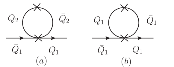
where and are respectively the complete fermion and gauge boson propagators, whereas and indicate their bare parts. Note that we are not writing the Lorentz indices and momentum integrals. In Eq.(21) is the sum of all two-particle irreducible vacuum diagrams, shown in Fig.(1), and can be analytically represented by
| (22) |
where is the fermion proper vertex. The most important property of this potential is that its minimization with respect to the complete propagators ( or ) lead to the fermionic or bosonic SDE cjt , i.e. the minimum conditions
| (23) |
reproduce exactly the SDE for the complete and propagators.
The physically meaningful quantity that at end is going to be related to a possible effective theory is the vacuum energy density given by
| (24) |
The fermion propagator in terms of the self-energy is , where . Expanding Eq.(24) in powers of we obtain cjt ; natale
| (25) |
In the case of massless fermions has no contribution of terms proportional to , what can be verified expanding in powers of the self-energy .
It is important to recall that taking into account the structure of the real vacuum, the propagator is a fermion bilinear and is a gap equation depending on two momenta, i.e. . Supposing that the expectation value of the fermion bilinear has the following operator expansion cs
| (26) |
where is a -number function, and acts like a dynamical effective scalar field. According to this we can expect that the gap equation may be approximated by
| (27) |
where is related to the Schwinger-Dyson equation and an effective field that is going to appear in the effective action as a variational parameter whose minimum will be indicated in the following by , corresponding to the leading contribution of its expansion around . Details of this approach can be seen in Ref.cs , but the point that we want to call attention next is what happens to the term proportional to .
The contribution to ,for instance in the case, now indicating the momenta integrals, is proportional to
| (28) |
In the above expression we can recognize the fermionic SDE between brackets:
| (29) |
therefore is identical to zero as long as we do have a self-energy that minimizes the vacuum energy. Note that the dependence of has been obtained as an expansion of the potential in powers of , and the disappears just if is the actual solution of the linear SDE, although the full potential is minimized by the complete non-linear SDE solution.
It may be argued that in ordinary calculations, if we work with a poor approximation for the self-energy, the equality of Eq.(29) may not hold, and the final result of is totally dependent on how reliable is the ansatz for in the full range of momenta. For realistic theories, corresponding to a true minimum of energy, the cancellation in Eq.(28) is exact, and the effective theory must not have a term. We should not introduce a quadratic mass term into an effective composite scalar Lagrangian only due to our inability of computing the actual self-energy. Of course, if we just work with an effective Lagrangian to describe the composite theory, it is clear that a polynomial in terms of the effective composite scalar field starting at can always be approximated by a potential starting at .
We have just argued that a theory leading to composite scalars has effective terms like suppressed. As we discuss since the beginning we are considering all possible behaviors of the fermionic self-energies, appearing when assume values from to , and when discussing the scalar mass determination in the context of the Bethe-Salpeter equation it was stressed how important is the wave function normalization, and how this condition is responsible for diminishing the scalar mass depending on the asymptotic behavior of the self-energy. We can now discuss how this effect appears in the effective potential approach. As commented in Refs.us5 , depending on the theory dynamics, when the self-energy decreases slowly with the momentum, i.e. in the case where approaches zero in Eq.(4), it is of fundamental importance the calculation of the effective Lagrangian kinetic term.
The kinetic term is given by the polarization diagrams (), shown in Fig.(2). In the effective action the kinetic term is the one whose denominator has the smallest power of the momentum, therefore being the most dependent on a self-energy slowly decreasing with the momentum. It gives origin in the effective Lagrangian to a contribution that looks like
| (30) |
however when the diagrams of Fig.(2) are calculated it is possible to see that this term will be multiplied by a non-trivial function () of the number of colors of the underlying theory (), the number of fermions (), and . This non-trivial function, that must normalize the scalar composite field, is obtained from cs
| (31) |
and the expansion around gives
| (32) |
which after some algebra can be written as us5
| (33) |
where the index is the parameter appearing in Eq.(4).
Eq.(33) has been calculated in Ref.us5 in the limits and and the results are equal to
| (34) |
when and
| (35) |
for the case .
The effective Lagrangian for the composite scalar bosons can be written as
| (36) |
where, making explicit the different contributions in terms of the variational field , we have
| (37) |
Eq.(37) differs from an ordinary scalar field Lagrangian by the factor that multiplies the kinetic term, therefore the final effective Lagrangian comes out when we normalize the scalar field according to
| (38) |
leading to the following normalized Lagrangian
| (39) |
The final effective theory for scalar composite fields can be written in the different limits, i.e. and , whose normalized couplings () are given respectively by us5
| (40) | |||||
| (41) |
and
| (43) |
where is the coupling constant of the strong (or technicolor) interaction that forms the scalar composite, and we have to consider expanded near the limits and .
The scalar mass obtained from the effective potential (Eq.(39)) at the minimum is
| (44) |
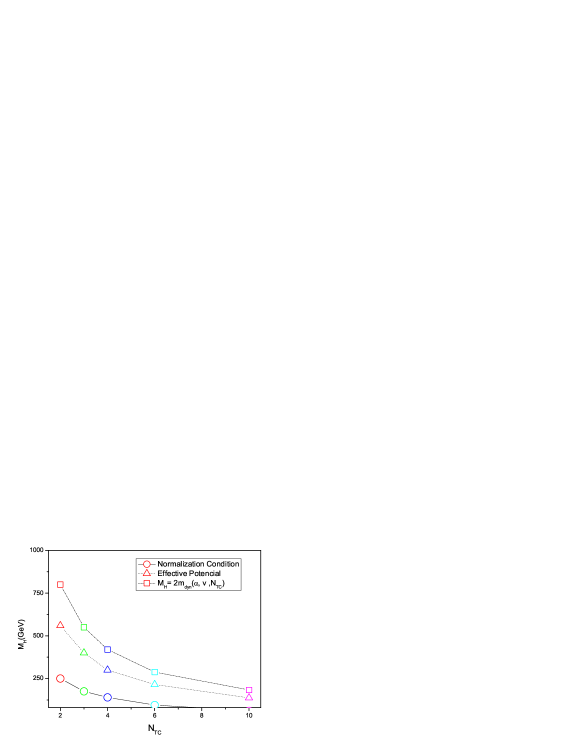
In Fig.(3) we show the differences in the scalar mass calculation using different approaches: BSE, effective potential and QCD like estimate (i.e. Eq.(10)). We consider strongly interacting theories with a large number of fermions. The number of fermions was chosen to be near a critical number, that for each TC group, is the number of fermions on the border of the conformal window ds ; us31
where respectively for to . The differences between the scalar masses computed within the BSE and the effective potential approaches are smaller than for small and decreases as is increased. The difference can be credited to the approximations performed when computing the effective potential for composite operators, being the crudest approximation the introduction of a very simple self-energy ansatz like the one of Eq.(4) into the loop expansion, remembering that this ansatz may be reasonable at small and large momenta, but certainly a crude approximation at intermediate momenta.
We conclude saying that, no matter we compute the scalar composite mass within the Bethe-Salpeter or in the effective potential approach, we obtain consistently small scalar masses only in the limit of a quite hard (in momentum space) self-energy. The scalar mass scales differently as we vary the dynamics of the theory, i.e. , , and . Nowadays there are many reasons takeuchi ; kondo ; us3 ; us12 ; frezz to believe that the self-energy may vary approximately as Eq.(4) when we change the parameter from to . Moreover, the effective Lagrangian describing composite scalars fields should not contain a quadratic term in the scalar field if we start from a strongly interacting theory with massless fermions, contrarily to what is assumed in many discussions about composite Higgs physics. As we commented in the introductory section of this work we consider the problem of generating one light composite scalar in a strongly interacting non-Abelian gauge theory assuming some mechanisms developed during the recent years, in particular in the Sections 2 and 3 we described in detail the main mechanisms developed for generating at least one light composite scalar in a theory with a unique characteristic scale . However, the mass of a composite Higgs boson can be modified by effects inherent to the nature of the strong interaction, as, for example, due to a strong mixing between the scalar mesons as could be expected to occur in QCD, or modified in the presence of other interactions that are not responsible for forming the composite scalar state. In order to evaluate the implications of these possibilities and how they could change the previous results we will present in Sections 4 and 5 a brief discussion about such possibilities.
IV A note about the mixing with techniglueballs and heavier scalars
In a strongly interacting gauge theory with massless fermions in the fundamental representation we have a global chiral symmetry, which is going to be spontaneously broken by a bilinear condensate, as happens in Eq.(1) in the case of the quark condensate. For a large number of fermions we shall have a large number of scalars and () pseudoscalars corresponding to the broken generators. Even in isolation there is no symmetry to impede the different scalars to mix, and this may modify the mass predictions discussed in the previous subsections. This would be the most naive way to obtain a small scalar mass if we have an appropriate mixing between the different scalars. However, this may be also the most difficult problem if we consider that this mixing is not even fully understood in the case of the QCD scalar spectra, and it is exactly based on what is known about this spectra, that we make a few comments on the possibility of obtaining a light scalar in any ordinary strongly interacting gauge theory.
Supposing that we have two ordinary scalars in the theory, namely and , the most simple mixing term in an effective Lagrangian would be
| (45) |
Assuming the lightest scalar formed by a fermion-anti-fermion pair, we can now suppose that may be a heavier scalar composite. This heavier composite may also be formed with a fermionic pair, but we cannot exclude the possibility that this one is the lightest scalar formed by strongly interacting gauge bosons, or what we may call a techniglueball. It is straightforward to verify that the mass, supposed to be the one computed according to the approaches discussed previously, will be modified only if we have a large mixing, i.e. a large value for in Eq.(45).
In the QCD case, the mixing of the QCD “Higgs” composite, i.e. the , with heavier scalars and with glueballs has been voiced for many times, see for instance Ref.mix1 ; mix2 ; mix3 ; mix4 ; mix5 ; mix6 . The present status of light composite scalar mesons in QCD can be also seen in the note by Amsler et al. in Ref.pdg . A strong mixing between the scalar mesons, and in particular the and the lightest glueball has not been observed in lattice simulations lat , although these results still need further improvements. Therefore, we cannot foresee any particular reason for groups, different from and originating a composite scalar boson, to have a large scalar mixing that could change the scalar mass values () discussed up to now. Even if there is mixing among scalars in QCD, it is clear that no matter is the underlying mechanism it does not lead to scalar masses lower than the QCD characteristic scale.
V Scalar composite boson in the presence of other interactions
The mass of a composite Higgs boson is modified in the presence of other interactions, i.e. any interaction that is not the one responsible for forming the composite scalar state. The prototype of such case has been discussed in Ref.foadi , where the SM is added to a technicolor theory, and the heavy top quark mass () is responsible for the decreasing of the original scalar mass. This is easy to understand since the observed composite Higgs mass () is the scalar mass resulting from the technicolor or strong theory () computed above minus a one-loop fermionic correction originated from the top quark loop:
| (46) |
In Eq.(46) the positive corrections to the composite Higgs mass, proportional to the SM gauge boson masses ( and ), can be neglected compared to the top quark mass correction. According to Ref.foadi the term can be large enough to reduce the scalar mass in order to have a composite Higgs boson as light as GeV.
The scenario described above works if the number of flavors of the technicolor or new strong interaction is , when the breaking of the global chiral symmetry will lead only to Goldstone bosons, which are going to provide the longitudinal component to the and bosons. In the case of , when the chiral symmetry is broken down to , there are going to remain Goldstone bosons or technipions. Actually, these bosons are going to be pseudo-Goldstone bosons, since they will acquire mass in a realistic extended technicolor theory. Technipion masses in several models are already excluded by LHC data up to twice the top quark mass chi . Massive technipions contribute to the scalar mass, and they contribute at the loop level to the mass given by Eq.(46)! About these corrections we can make a comparison with QCD: These are the “massive” pion loop contributions to the meson mass. For QCD in isolation these corrections are zero, since the pions are massless. As we consider current quark masses the pions obtain a small mass and the meson mass has small corrections due to the small and quark masses. Of course, we are considering that the has a minor contribution from heavier quarks and mixing with glueballs. A discussion about loop corrections to the mass can be seen in Ref.nat .
Let us now turn to technicolor with . In this case Eq.(46) will be transformed into
| (47) |
where is the technipions (or pseudo-Goldstone) masses. The determination of , and even its signal, in Eq.(47) is quite model dependent. It will involve the scalar self-couplings and the scalar technipions coupling, what may not be necessarily small numbers just based on the linear sigma model type of calculation nat . Assuming that the scalar system is described by a linear sigma model, and will be of the order of , which is not a small number nat , and assuming the model dependent limit of Ref.chi we can estimate
| (48) |
If we just imagine that the observed Higgs boson should be a composite particle, our naive estimate indicates that the presence of the heavy top quark may not be enough to lower the composite scalar mass to the observed value.
There is another quite important fact that is missing in the effective Lagrangians when SM fermions, as the top quark, are introduced into the calculations: They generate an effective interaction in the effective potential for composite operators. This was observed for the first time in the QCD effective Lagrangian in Ref.bar , and in technicolor models this contribution was calculated by us us5 without a thorough analysis of the consequences.
The contribution to the effective Lagrangian due to the ordinary massive fermions is given respectively by the diagram of Fig.(4), where the effective coupling is determined through Ward identities as discussed in Refs.soni ; soni2 ; doff3 , and such coupling will be given by
| (49) |
where is the weak coupling and is an ordinary fermion (or quark) self-energy.
A full computation of ordinary fermion masses requires the introduction of an extended technicolor interaction (ETC). Without knowing the ETC theory the best that we can do is to compute the effect of ordinary fermions to the effective potential as a function of their masses. The trilinear contribution to the effective potential due to the presence of ordinary fermion masses can be computed as discussed in Refs.us5 ; bar , or we can compute the trilinear coupling as performed by Carpenter et al. soni . Indicating the trilinear contribution to the effective Lagrangian as , we recover from us5 the largest trilinear coupling as
| (50) |
This is the largest contribution to the trilinear coupling, and it was obtained in the limit of Eq.(4). The details of the calculation are in the appendix of Ref.us5 .
The contribution to the effective potential is the one that may decrease the scalar mass, and is the equivalent of the negative top quark contribution in Eq.(46). However this coupling must be compared to the quadrilinear contribution to the potential (see us5 ), which has the same effect of the technipions self-coupling present in Eq.(47). It is the balance between these different couplings that will lower or increase the scalar composite mass.
In simple words we may say that the contribution of ordinary fermions, even considering the effect of the top quark mass in Eq.(50) com1 , is small due to the presence of the weak coupling and the other numerical factors, and hardly compete with larger terms (and ) of , characteristic of the composite scale (), and which are responsible for the determination of the composite scalar boson mass. A precise calculation must involve specific models, and at this level we may say the the top quark effect may lower the composite scalar mass, but at the cost of precise cancellation of different terms in the effective Lagrangian. The most we can learn from this discussion is that with a heavy top quark, and in the presence of massive technifermions, the trilinear terms in the effective composite scalar Lagrangians cannot be always neglected in the study of phenomenological models.
VI Light composite scalar boson in two-scale TC models
One possibility for generating a light composite scalar happens in the case where we have at least two composite bosons (, and they have a strong mixing ff . In this case we may have a see-saw mechanism where one of the scalar composites may turn out to be quite light. The main problem along this line is to find the condition for the existence of this strong mixing in the case where we have several composite scalar bosons. In a single theory with a unique scale, as we discussed before, we do not know of any mechanism in this direction. Therefore we shall consider a two-scale model where it is simple to verify why a strong mixing between scalar composite appears, and speculate how this mechanism can be extended to other cases usx .
Consider the formation of a light composite scalar boson when the TC theory features two technifermion species in different representations, and , under a single technicolor gauge group, with characteristic scales and . Walking technicolor theories can have fermions belonging to different technicolor representations and, therefore, may have two different scales with characteristic chiral symmetry breaking scales . Here we assume that technifermions are in the representations and under a single technicolor gauge group as described in Ref.Lane . In the model proposed by Lane and Eichten, it is assumed that the TC running coupling constant is given by
where , sus and and are technifermions doublets in the representation . Note that the and doublets of technifermions belong to the complex TC representation and , with dimensionality . For a large enough number of doublets it is possible to obtain Lane (or the decay constant ) because
| (51) |
in this case we can assume that the asymptotic technifermions self-energy behavior in representation can be described by Eq.(4), this hypothesis can be verified with the numerical results obtained in Lane .
At low energies we have an effective theory containing two different sets of composite scalars and , like the ones described in Ref.Lane . We will assume an ETC gauge group containing technifermions doublets in the fundamental representation , and technifermions doublets, assuming for representations (2-index antisymmetric , 2-index symmetric ). The phenomenology of these type of models was already described in Ref.Lane .
The fermionic content of the model that we discuss in this section has two multiplets of technifermions in the representations and of the type
| (60) |
where is a technicolor index and is a flavor index. In this type of theory the ETC group would be , and in order to incorporate the mixing between and , we must take into account the contributions of the ETC as displayed in Fig.(5). Remembering that the self-energy can also be related to the solutions of the Bethe-Salpeter equation, we can observe that the scalar boson , formed by the fermions in the representation receive contributions of the condensates of the two different representations, as shown in Fig.(5).
We can detail a little bit more the comment of the previous paragraph and the behavior of the diagrams in Fig.(5). The techniquarks will receive a dynamical mass due to the usual TC contribution and to the two diagrams in Fig.(5), that we indicate by
| (61) |
where and are calculable constants. In the above expression the first one is the usual TC contribution due to condensation of techniquarks in the representation . The second comes from the ETC interaction with techniquarks that condensate in the representation and the third one is the contribution from ETC interactions. Suppose now that the techniquarks self-energy does not have a walking behavior, or a slow decrease with the momentum i.e. is given by Eq.(4), therefore the ETC contribution to , Fig.(1b) will be given by us3
| (62) |
which is totally negligible.
We can now consider the effect of technifermions in the representation . This contribution is represented by the diagram of Fig.(5a), where we may have an extreme walking behavior for the technifermions. In this case the correction due to ETC will be dominated by a self-energy of the type given by Eq.(8) resulting in us3
| (63) |
Therefore the ETC correction () plays a role similar of a bare mass term for the self-energy, i.e. a very hard self-energy! A similar reasoning may also be applied to the . Although only one of the technifermions representations of one given TC group has a walking behavior and this group belongs to an ETC theory, at the end both technifermions representations will have asymptotically hard self-energies. In the following we will consider that the technifermions associated to the representation are in the fundamental representation with a self-energy behaving as the one of Eq.(7), and behaving as Eq.(8) .
The argumentation about the origin of a strong mixing between the two composite scalars will be discussed in terms of the different contributions to the CJT potential, and as will be explained in the sequence, this mixing will be enhanced only if one of the self-energies decreases slowly with the momentum.
The different terms that are going to appear in the effective action of the composite scalar system are momentum integrals of different powers of the self-energies cjt , which are going to be represented as , where acts like a dynamical effective scalar field (expanded around its zero momentum value) us5 ; cs , and it is interesting to verify how it is going to be the behavior of the term (as a function of the momentum), which is the leading term of the effective potential us5 ; cs .
The fourth power of the self-energy associated to the fields and , where the index will be related to technifermions with (in principle) a soft self-energy (), and the index will be related to technifermions in a representation or , with a hard self-energy (), will be written as
| (64) | |||||
| (65) |
where we defined and is the ratio of Casimir operators and couplings of Eq.(63).
After some lengthy calculation, that follows the same steps delineated in Ref.us5 , we obtain the following effective Lagrangian using the self-energies described previously
| (66) | |||||
The coefficients, to , shown in equation above are described in Ref.usx .
The most important characteristic of this effective Lagrangian is the mixing term
| (67) |
This mixing is the one that defines the splitting between the effective fields and , as discussed by Foadi and Frandsen ff , whereas within the approach taken in this work their parameter ff , characterizing the mixing in the mass matrix, is
| (68) |
We emphasize that this mixing appears naturally in a two-scale TC model, where it is enough that one of the scales, and the fermionic representation associated to it, has an extreme walking behavior and the TC group is embedded into an ETC theory.
Considering , we note that the scale is defined by
| (69) |
which leads to
| (70) |
Finally, assuming
| (71) |
we obtain
| (72) |
We can write the following mass matrix in the base formed by the composite scalars () and ()
| (75) |
The eigenvalues of this matrix provide the mass spectrum for the light scalar and heavy , including the mixing effect parametrized by , where
| (76) |
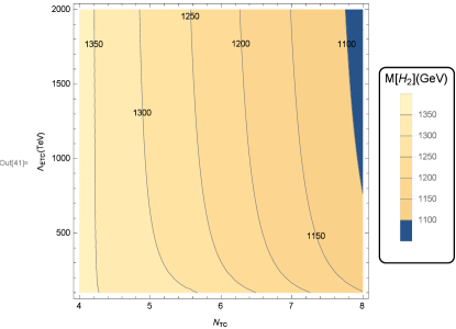
From the above equations we can determine the mass spectrum for the scalar bosons, and , which are the diagonalized masses of the scalars and . As an example we present the mass spectrum obtained for the light and heavier composite scalars and in the cases where , ( Fig. (6)).
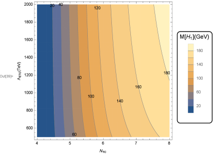
We computed an effective action for a composite Higgs boson system formed by two technifermion species in different representations, and , under a single technicolor gauge group with characteristic scales and as the original proposal presented in Ref.Lane . The calculation is based on an effective action for composite operatorsus5 , the novelty of the calculus presented in this section is that we included technifermions in different representations, and , under a single technicolor gauge group. The mixing between the composite scalar bosons and can generate a light Higgs boson of mass of approximately GeV. To obtain a large mixing it is enough that one of the technifermions representations has a walking behavior and the TC group is embedded in an ETC theory. At the end the technifermions of both representations will have asymptotically hard self-energies.
For a set of parameters similar to the ones used in Ref.Lane in the case , we obtain the same TC group necessary to generate the walking behavior, , leading also to small scalar masses. Furthermore, the large anomalous dimensions enhance light-scale technipion masses, , where technirho mass . The difference between the results obtained for the representations and (see Ref.usx ) is that in the case we obtain a light scalar mass only with a large ETC scale . For the heavy scalar bosons obtained with or we expect the mass to be in the range GeV. Concluding that a light composite scalar boson mass can be generated in a type of see-saw mechanism in a two-scale TC model.
Note that the main reason for generating a strong mixing between the effective composite scalar fields appears in Eqs. (64) and (65), leading to the mixing term in the effective potential (see Eq.(66)). If the self-energies of the different techniquarks were soft the composite scalars barely mix, however if one of the self-energies is of the hard type it is enough to generate a strong mixing and a light scalar. Of course, if one the self-energies decreases slowly with the momentum the condition for a light scalar existence is already in there. Looking at this it may be considered that we introduced a very complicated model just to obtain a light scalar, but it should be remembered that we do have in this case an extra possibility to manipulate the scalar masses values, i.e. we can obtain an even larger mass splitting between different composite scalar boson masses than the one obtained in the case when we just have only one hard self-energy.
VII The case of many composite scalars
It is possible that the mixing mechanism that we discussed in the previous section may be extended to models with more than one TC group, although it is also possible to envisage that in this case we shall need a more complex ETC interaction in order to mix the different groups. This possibility may occur under two conditions: The first one is that one of the scalar composites is formed by fermions of a given group and representation such that their self-energy is of the extreme walking type. The second one imply in a strong mixing between the different scalar composites, this will happens if the different scalar bosons interact through an ETC generating effective four-fermion interactions like the ones displayed in Fig.(5).
As one example, suppose that we have several TC groups, , ,… We must have at least one of the with a walking behavior, and this one be embedded into an ETC theory together with some of the others TC groups, which may be characterized by a high energy scale and standard soft self-energy, leading to very massive composites. The fact that they mix through ETC interactions will generate a see-saw mechanism, in such a way that at least one of the scalar composites will become quite light, when compared to the mass scales of all other TC theories.
The most economical case will happens when the light composite states will belong to an group, with technifermion doublet, providing exactly the degrees of freedom necessary to break the electroweak group and generating only one light scalar composite, as seems to be the experimental scenario observed up to now. The group that we are referring about does not necessarily should have an almost conformal dynamical behavior, but it must mix with another TC group endowed with an extreme walking behavior, and this mixing has to be tuned in order to provide exactly the degrees of freedom necessary to implement the weak boson masses and generate a light scalar boson. All the other composite states may be quite heavy and not accessible to the LHC energies.
VIII Remark on vector composites
There is a large amount of phenomenology describing the possibility of observing vector composites, like the technirho or techniomega. However it is interesting to recall the remark made by some of us in Ref.us4 that the vector composites are not going to be light, are not going to be modified by the dynamics that leads to light scalars, and may be difficult to observe at the LHC. The vector composites in a non-Abelian gauge theory are quite massive basically due to the spin-spin part of the hyperfine interactions. For waves the hyperfine splitting has been determined as ei1 ; ei2
| (77) |
where is the meson wave function at the origin. We also assume that the fermion masses forming the vector boson are equal to the dynamical mass . Eq.(77) has been derived in the heavy quarkonium context ei1 ; ei2 , although it seems to work reasonably well even in the presence of light fermions sc .
Assuming as the worst possibility that what is consistent with a frozen infrared coupling constant freezing1 ; freezing2 ; freezing3 ; freezing4 , the fact that no other composite scalar boson has been found below GeV, and that , what is consistent with Eq.(3), we obtain the following inequality from Eq.(77)
| (78) |
With the dynamical fermion mass values (or characteristic TC scales ) that we have discussed in this work, the vector composite masses are going to be heavy and with a quite model dependent phenomenology. The main point of this section was to recall that possibly the experimental signal of vector composites will hardly be affected by the specific dynamics of the self-energies that we discussed up to now, and probably the ratio between scalar and vector masses will not be helpful to reveal the underlying strong interaction dynamics.
IX Results and conclusions
We discussed the possibilities for generating a light composite scalar boson in non-Abelian strongly interacting gauge theories. In Sections 2 and 3 this problem was studied with two different approaches: The solutions of Bethe-Salpeter equations and the effective potential for composite operators. Both approaches lead to the same result, indicating that light composite scalar bosons appear as a direct consequence of extreme walking (or quasi-conformal) technicolor theories, where the asymptotic self-energy behavior is described by Eq.(8)(or ).
In the BSE approach the extreme walking behavior of fermionic self-energies and the wave function of scalar bound states are dominated by higher order interactions and are characterized by a much harder decrease with the momentum, and in this case the normalization condition of the BSE do constrain the scalar masses, resulting in a light composite scalar boson.
In the effective potential approach the normalization constant is important to set the right scale in our effective Lagrangian, the scalar mass obtained in this approach is proportional to this constant, see Eq.(44), in the extreme walking behavior () we obtain , where is the normalization factor calculated with , which is associated to the known asymptotic self-energy behavior predicted by the operator product expansion (OPE). The consequence of the extreme walking behavior is the reduction of the scalar composite boson mass by almost one order of magnitude.
In Section 3 we commented that quadratic terms are not natural in effective Lagrangians generated through the calculation of the effective potential for composite operators, where they may appear only when poor approximations for the self-energies are used to compute the effective action. We also show that the scalar boson mass scales differently with the theory parameters (such as and ) according to the theory dynamics, i.e. according to the different self-energies behavior.
In the Section 5 we discussed how the mass of a light composite scalar boson can be modified in the presence of other interactions, i.e. any interaction that is not the one responsible to form the composite scalar state, as an example we consider the prototype discussed in Ref.foadi , where the SM is added to a technicolor theory and the heavy top quark mass () is responsible to decrease the original scalar mass. This case is realistic when the strongly interacting theory is a minimal one. When the strong or TC theory has a larger chiral symmetry, there will remain many pseudo-Goldstone bosons, and they will contribute to the scalar mass with a signal contrary to the one of the top quark. In the effective potential for composite operators these new interactions will be responsible for new cubic and quartic interactions.
In the Section 6 we considered the possibility of generating a light composite scalar where we have at least two composite bosons and they have a strong mixing, to obtain a large mixing it is enough that one of the technifermions representations has a extreme walking behavior and the TC group is embedded in an ETC theory. In this case we have a see-saw mechanism where one of the scalar composites turn out to be quite light, and we obtain a light scalar boson mass of approximately a few hundred GeV. In Section 7 we presented a brief discussion about how the mixing mechanism, presented in the Section 5, can be extended to models with more than one TC group, and in Section 8 we remark that vector composites masses are not going to be affected by the mechanisms that help to lower the scalar mass, since most of their masses are originated by the spin-spin interaction, and if there is any new strongly interaction at the TeV scale the vector composites may scape detection in the near future.
Summarizing, in this work we identified that, regardless of the approach used for generating a light composite scalar boson, the behavior exhibited by the extreme walking (or quasi-conformal) technicolor theories is the main feature needed to produce a light composite scalar boson, i.e. a mass roughly one order of magnitude below the characteristic mass scale of the strongly interacting theory responsible for its formation. It is also interesting to note, according to what was presented in Section 5 (and 6), that a strong mixing between composite scalars may appear in the presence of several strongly interacting theories, leading to a see-saw mechanism and a light composite scalar bosons, just if one of the theories has a walking behavior, which is going to be transmitted to the other theories if they are embedded into a large ETC theory. In all the cases it seems that a slowly decreasing self-energy with the momentum is a necessary condition for the new fermions of a strongly interacting theory to form a light composite scalar.
Acknowledgments
This research was partially supported by the Conselho Nacional de Desenvolvimento Científico e Tecnológico (CNPq) by grants 442009/2014-3 (AD) and 302884/2014-9 (AAN), by the Coordenação de Aperfeiçoamento de Pessoal de Nível Superior (CAPES) (AAN), and by Fundação de Amparo á Pesquisa do Estado de São Paulo (grant 2013/22079-8).
References
- (1) ATLAS Collaboration, Phys. Lett. B 716, 1 (2012).
- (2) CMS Collaboration, Phys. Lett. B 716 30 (2012).
- (3) F. Sannino, Int. J. Mod. Phys. A 20, 6133 (2005).
- (4) Y. Nambu and G. Jona-Lasinio, Phys. Rev. 122, 345 (1961).
- (5) R. Delbourgo and M. D. Scadron, Phys. Rev. Lett. 48, 379 (1982).
- (6) N. A. Tornqvist and M. Roos, Phys. Rev. Lett. 76, 1575 (1996).
- (7) N. A. Tornqvist and A. D. Polosa, Nucl. Phys. A 692, 259 (2001).
- (8) N. A. Tornqvist and A. D. Polosa, Frascati Phys. Ser. 20, 385 (2000).
- (9) B. Bellazzini, C. Csáki and J. Serra, Eur. Phys. J. C 74, 2766 (2014).
- (10) Kenneth Lane, Phys. Rev. D 90, 095025 (2014).
- (11) ATLAS and CMS Collaboration, Phys. Rev. Lett. 114, 191803 (2015).
- (12) A. Doff and A. A. Natale, Phys. Lett. B 537, 275 (2002).
- (13) Roshan Foadi and Mads T. Frandsen, arXiv:1212.0015v1.
- (14) A. D. Polosa, N. A. Tornqvist, M. D. Scadron and V. Elias, Mod. Phys. Lett. A 17, 569 (2002).
- (15) R. Delbourgo and M. D. Scadron, J. Phys. G 5, 1621 (1979).
- (16) A. Doff and A. A. Natale, Phys. Lett. B 677, 301 (2009).
- (17) A. Doff and A. A. Natale, Phys. Rev. D 68, 077702 (2003).
- (18) H. D. Politzer, Nucl. Phys. B 117, 397 (1976).
- (19) J. M. Cornwall and R. C. Shellard, Phys. Rev. D 18, 1216 (1978).
- (20) A. Doff, F. A. Machado and A. A. Natale, Annals of Physics 327 1030 (2012).
- (21) A. Doff, F. A. Machado and A. A. Natale, New. J. Phys. 14, 103043 (2012).
- (22) A. Doff, E. G. S. Luna and A. A. Natale, Phys. Rev. D 88, 055008 (2013).
- (23) L.-N. Chang and N.-P. Chang, Phys. Rev. D 29, 312 (1984).
- (24) L.-N. Chang and N.-P. Chang, Phys. Rev. Lett. 54, 2407 (1985).
- (25) N.-P. Chang and D. X. Li, Phys. Rev. D 30, 790 (1984).
- (26) J. C. Montero, A. A. Natale, V. Pleitez and S. F. Novaes, Phys. Lett. B 161, 151 (1985).
- (27) P. Langacker, Phys. Rev. Lett. 34, 1592 (1975).
- (28) R. Frezzotti and G. C. Rossi, Phys. Rev. D 92, 054505 (2015).
- (29) K. Lane, Phys. Rev. D 10, 2605 (1974).
- (30) S. Mandelstam, Proc. R. Soc. A 233, 248 (1955).
- (31) C. H. Llewellyn Smith, Nuovo Cimento, A 60, 348 (1969).
- (32) A. Doff, A. A. Natale and P. S. Rodrigues da Silva, Phys. Rev. D 80, 055005 (2009).
- (33) T. Takeuchi, Phys. Rev. D 40, 2697 (1989).
- (34) K.-I. Kondo, S. Shuto and K. Yamawaki, Mod. Phys. Lett. A 6, 3385 (1991).
- (35) T. Nunes da Silva, E. Pallante and L. Robroek1, arXiv:1506.06396 [hep-th].
- (36) V. Elias and M. D. Scadron, Phys. Rev. Lett. 53, 1129 (1984).
- (37) H. Pagels and S. Stokar, Phys. Rev. D 20, 2947 (1979).
- (38) T. Karavirta, J. Rantaharju, K. Rummukainen and K. Tuominen, JHEP 1205, 003 (2012).
- (39) M. Hayakawa, K. I. Ishikawa, S. Takeda and N. Yamada, Phys. Rev. D 88, 094504 (2013).
- (40) T. Appelquist et al., Phys. Rev. Lett. 112, 111601 (2014).
- (41) T. Appelquist and L. C. R. Wijewardhana, Phys. Rev. D 36, 568 (1987).
- (42) We assume that in TC models, due to the phenomenon of dynamical technigluon mass generation, in similarity with QCD, the coupling constant will freeze in the infrared to moderate values. A discussion about this possibility in QCD can be seen in J. M. Cornwall, Center vortices, the functional Schrodinger equation, and CSB, Invited talk at the conference “Approaches to Quantum Chromodynamics”, Oberwölz, Austria, September 2008, arXiv:0812.0359 [hep-ph].
- (43) A. C. Aguilar, A. Mihara and A. A. Natale, Phys. Rev. D 65, 054011 (2002).
- (44) P. Hoyer, arXiv:1409.4703 [hep-ph].
- (45) J. D. Gomez and A. A. Natale, arXiv:1509.04798 [hep-ph] and references therein.
- (46) T. A. Ryttov and Francesco Sannino, Phys. Rev. D 78, 065001 (2008).
- (47) J. M. Cornwall, R. Jackiw and E. Tomboulis, Phys. Rev. D 10, 2428 (1974).
- (48) A. Doff, A. A. Natale and P. S. Rodrigues da Silva, Phys. Rev. D 77, 075012 (2008).
- (49) W. A. Bardeen, FERMILAB-CONF-95-391-T.
- (50) M. Heikinheimo, A. Racioppi, M. Raidal, C. Spethmann and K. Tuominen, arXiv:1304.7006 [hep-ph].
- (51) A. A. Natale, Nucl. Phys. B 226, 365 (1983).
- (52) J. Nebreda, J. T. Londergan, J. R. Pelaez and A. P. Szczepaniak, arXiv:1403.2790 [hep-ph].
- (53) L. Montanet, Nucl. Phys. Proc. Suppl. 86, 381 (2000).
- (54) S. Narison, arxiv:0208081 [hep-ph].
- (55) H. G. Dosch and S. Narison, Nucl. Phys. Proc. Suppl. 121, 114 (2003).
- (56) J. R. Pelaez, Phys. Rev. Lett. 92, 102001 (2004).
- (57) G. Mennessier, S. Narison and X.-G. Wang, Phys. Lett. B 696, 40 (2011).
- (58) J. Beringer et al. (Particle Data Group), Phys. Rev. D 86, 010001 (2012).
- (59) A. Hart, C. McNeile, C. Michael and J. Pickavance, Phys. Rev. D 74, 114504 (2006).
- (60) R. Foadi, M. T. Frandsen and F. Sannino, Phys. Rev. D 87, 095001 (2013).
- (61) R. S. Chivukula, P. Ittisamai, E. H. Simmons, J. Ren, Phys. Rev. D 84, 115025 (2011); Erratum-ibid. D 85, 119903 (2012).
- (62) N. A. Tornqvist, Nucl. Phys. B (Proc. Suppl.) 74, 159 (1999).
- (63) Barducci, A., Casalbuoni, R., DeCurtis, S. , Dominici, D. and Gatto, R., Phys. Rev. D 38, 238 (1988).
- (64) J. Carpenter, R. Norton, S. Siegemund-Broka and A. Soni, Phys. Rev. Lett. 65, 153 (1990).
- (65) J. D. Carpenter, R. E. Norton and A. Soni, Phys. Lett. B 212, 63 (1988).
- (66) A. Doff and A. A. Natale, Phys. Lett. B 641, 198 (2006).
- (67) Note that the enhancement due to the top quark mass that we refer here is how its large mass acts in the sense of decreasing the scalar composite mass.
- (68) A. Doff and A. A. Natale, Phys. Lett. B 748, 55 (2015).
- (69) K. Lane and E. Eichten, Phys. Lett. B 222, 274 (1989).
- (70) S. Raby, S. Dimopoulos and L. Susskind, Nucl. Phys. B 169, 373 (1980)
- (71) E. Eichten, K. Gottfried, T. Kinoshita, K. D. Lane and T. M. Yan, Phys. Rev. D 17, 3090 (1978).
- (72) E. Eichten, K. Gottfried, T. Kinoshita, K. D. Lane and T. M. Yan,T, Phys. Rev. D 21, 203 (1980).
- (73) H. Schnitzer, invited talk at Conf. on Hadron Spectroscopy (Univ. Maryland, March 1985), preprint BRX-TH-184.