Proximal extrapolated gradient methods for variational inequalities

Abstract

The paper concerns with novel first-order methods for monotone variational inequalities. They use a very simple linesearch procedure that takes into account a local information of the operator. Also the methods do not require Lipschitz-continuity of the operator and the linesearch procedure uses only values of the operator. Moreover, when operator is affine our linesearch becomes very simple, namely, it needs only vector-vector multiplication. For all our methods we establish the ergodic convergence rate. Although the proposed methods are very general, sometimes they may show much better performance even for optimization problems. The reason for this is that they often can use larger stepsizes without additional expensive computation.

2010 Mathematics Subject Classification: 47J20, 65K10, 65K15, 65Y20, 90C33

Keywords: variational inequality, monotone operator, linesearch, nonmonotone stepsizes,
proximal methods, convex optimization, ergodic convergence.

1 Introduction

This paper considers a problem of the variational inequality in a general form

$$\text{find }x^{*}\in\mathcal{E}\colon\quad\left\langle F(x^{*}),x-x^{*}\right\rangle+g(x)-g(x^{*})\geq 0\quad\forall x\in\mathcal{E},$$ (1)

where $F\colon\mathcal{E}\to\mathcal{E}$ is a monotone operator and $g\colon\mathcal{E}\to(-\infty,+\infty]$ is a convex function. This is an important problem that has a variety of theoretical and practical applications [19, 24, 18].

The main iteration step of the proposed method is defined as follows

$$y_{n} =x_{n}+\tau_{n}(x_{n}-x_{n-1})$$

$$x_{n+1} =\operatorname{prox}_{\lambda_{n}g}(x_{n}-\lambda_{n}F(y_{n})),$$

where we define $\tau_{n}$, $\lambda_{n}$, and $y_{n}$ from local properties of $F(y_{n})$. For this in each iteration we run some simple linesearch procedure. We propose different procedures for different cases: for a general problem (1), for (1) with $g(x)=\delta_{C}(x)$, and for a case when $F$ is a gradient of a convex differentiable function. Each iteration of the linesearch procedure requires only one value of $F$ and function $g$ is not used at all. In contrast to many known methods, we do not require monotonicity of stepsizes $(\lambda_{n})$. Also in case when $F$ is affine our linesearch procedures needs only vector-vector computation. Moreover, our analysis does not need a Lipschitz assumption on $F$, only locally Lipschitz one.

Although we consider quite a general problem, our discussion presented below consists from two separate parts devoted to the optimization problems and variational inequality problems. This is because we noticed that for some difficult optimization problems our algorithm may work much better than some existing methods. Next section after the introduction devotes to studying of our two methods. We show their globally convergence, consider some particular cases and establish complexity rates. In Section 3 we consider a problem of composite minimization for which we improve one of our methods. In Section 4 we study some known linesearch procedures and make numerical illustrations of our methods with several popular methods.

1.1 Preliminaries

In what follows, $\mathcal{E}$ denotes a finite-dimensional real vector space with inner product $\left\langle\cdot,\cdot\right\rangle$ and norm $\left\|\cdot\right\|$, $\nabla f$ denotes a gradient of a smooth function $f$. For a proper lower semicontinuous convex function $g\colon\mathcal{E}\to(-\infty,\infty]$ we denote its domain by $\operatorname{dom}g$, i.e., $\operatorname{dom}g:=\{x\in\mathcal{E}\colon g(x)<\infty\}$. The proximal operator $\operatorname{prox}_{g}\colon\mathcal{E}\to\mathcal{E}$ is defined as

$$\operatorname{prox}_{g}(y):=\operatorname{argmin}_{x\in\mathcal{E}}\bigl{\{}g(x)+\frac{1}{2}\left\|x-y\right\|^{2}\bigr{\}}.$$

For a set $C$, we denote by $\delta_{C}$ the indicator function of the set, that is, $\delta_{C}(x)=0$ if $x\in C$ and $\infty$ otherwise. A metric projector onto $C$ we denote as $P_{C}$. Clearly, by definition, $P_{C}x=\operatorname{prox}_{\delta_{C}}x$.

The operator $F$ is called monotone if

$$\left\langle F(x)-F(y),x-y\right\rangle\geq 0\quad\forall x,y\in\mathcal{E}.$$

1.2 Optimization perspective

Consider the following problem of composite minimization

$$\min_{x}\Phi(x):=f(x)+g(x),$$ (2)

where $f$ is a differentiable convex function, and $g$ is a proper lower semicontinuous convex function. Such formulation assumes that we know the structure of the underlying function $\Phi$. It is not difficult to verify that the first order optimality conditions of (2) are a particular case of (1) with $F=\nabla{f}$.

Problem (2) is rich enough to encompass many important applications in machine learning, image processing, compressed sensing, statistics, etc. [36, 38, 12, 48, 3, 16, 11]. Although first-order methods for problem (2) have a long history, they continue to receive much attention from optimization community. Many real-life applications are large-scale and in this case first-order methods often outperform other methods such as interior point methods, Newton methods, since the iterations of the former are much cheaper and do not depend on the dimension of the problem as much as the latter do.

Under the assumption that $\nabla f$ is Lipschitz-continuous, i.e., there exists some $L>0$ such that

$$\left\|\nabla f(x)-\nabla f(y)\right\|\leq L\left\|x-y\right\|,$$ (3)

one of the most simple methods for solving (2) is the proximal gradient method that generates $(x_{n})$ as

$$x_{n+1}=\operatorname{prox}_{\lambda_{n}g}(x_{n}-\lambda_{n}\nabla f(x_{n})),$$ (4)

where $\lambda_{n}\in(0,\frac{2}{L})$.

There are several methods [47, 13] that do not require condition (3). Our linesearch procedure in some sense is similar to them but is cheaper since it does not use a proximal mapping. The more extended discussion concerning this will be presented in Section 4. We underline that problems, where (3) does not hold, take place, for example, in barrier methods, entropy maximization, geometric programming, image processing [16, 15, 36, 5, 6, 42].

We also have to mention a very important class of two-step proximal gradient methods that include inertial (heavy ball) methods introduced by Polyak in [40] and accelerated proximal methods, pioneered by seminal work of Nesterov [35] and further developed in [36, 3, 48] for a problem of composite minimization. This class enjoys an improved convergence rate compared with classical proximal gradient method (4). For all these methods condition (3) is also important.

In order to see why assumption (3) is so crucial for most optimization methods, consider (4) in more detail. There are two classical approaches of deriving the proximal gradient method. The first one consists in the interpretation of (4) with fixed $\lambda=\lambda_{n}\in(0,\frac{2}{L})$ as forward-backward method. Condition (3) is necessary to establish that operator $\operatorname{Id}-\lambda\nabla f$ is firmly nonexpansive (Baillon-Haddad theorem [2]). After this we can simply deduce that $\operatorname{prox}_{\lambda g}(\operatorname{Id}-\lambda\nabla f)$ is averaged. Then a convergence of $(x_{n})$ to a minimizer of $\Phi(x)$ follows from the celebrated Krasnosel’skii-Mann theorem [2].

In order to derive (4) in a different way, we need the following inequality

$$|f(y)-f(x)-\left\langle\nabla f(x),y-x\right\rangle|\leq\frac{L}{2}\left\|x-y\right\|^{2}$$ (5)

that is well-known as descent lemma [2]. Note that this lemma holds for any smooth function $f$ that satisfies (3). We point out that analysis of accelerated proximal methods is much more sophisticated and it can not be interpreted as forward-backward splitting iteration. Nevertheless one of the main ingredients in their analysis is inequality (5) and hence the assumption (3) is also necessary for them.

Among first-order methods there has been always some trade-off between methods with fixed stepsize and ones with variable stepsizes. The former are simpler and require less computation per iteration, however, they require to know the Lipschitz constant $L$. Usually we are able only to estimate this constant from the above (and even this task sometimes can be very challenged), moreover this estimation is often quite conservative, so the method will use tiny steps. Methods with variable stepsizes in each iteration run some linesearch procedure in order to find appropriate stepsize. They are more flexible and usually allow to use larger steps than what is predicted by the Lipschitz constant. At this moment there are a lot of possible linesearch procedures and adaptivity techniques for (4) or some particular cases of (4), see [43, 1, 4, 47, 36, 3, 13, 37, 26].

Our method seems to fill in this trade-off: it is very simple, it uses variable and nonmonotone stepsizes, and linesearch procedure is quite cheap and flexible. This significantly differs it from the most known methods. For example, each inner iteration of the popular Armijo-like linesearch procedure for (4) proposed in [3] requires evaluation of $f$ and $\operatorname{prox}_{\lambda_{n}g}$. Moreover, in order to provide convergence of generated sequence $(x_{n})$, the sequence of stepsizes $(\lambda_{n})$ must be nonincreasing.

On the other hand, the flexibility of stepsizes $(\lambda_{n})$ in our methods causes difficulties to get a nonergodic convergence rate of the proposed algorithms. We hope the presence of numerical experiments in the paper makes this lack up. Roughly speaking, the general picture of applicability of our methods is the following. In cases when local Lipschitz constant of $\nabla f$ changes drastically, that is $f$ has very different curvature in different directions, then a global Lipschitz constant can not be a good prediction and our methods will benefit from using the local information of $\nabla f$. In turn, when $\nabla f$ is rather flat, i.e. local Lipschitz constant of $\nabla f$ does not change too much, our method will be in the worse case comparing to other methods, since the latter allow to take stepsizes larger or/and they may enjoy a better complexity rate. Clearly, the first case is the most difficult in optimization, since it includes problems with highly nonlinear $\nabla f$ or linear but ill-conditioned $\nabla f$.

1.3 Variational inequality perspective

This subsection concerns with a more general case when $F$ is not a gradient of a convex function. A general approach to solve (1) consist in solving of a sequence of the simpler variational inequalities [10, 21]. We concentrate ourselves on the most simple case of this approach: projected (proximal) methods.

When, for example, $F$ satisfies cocoercivity assumption (that is stronger than just monotonicity) then most methods from optimization framework can be still applied to this case. In particular, this holds for the proximal gradient method (forward-backward method) [39, 27], inertial method [33, 28]. However, those methods do not converge when $F$ is monotone.

When $g(x)=\delta_{C}(x)$, variational inequality (1) reduces to

$$\left\langle F(x^{*}),x-x^{*}\right\rangle\geq 0\quad\forall x\in C,$$ (6)

where $C\subseteq\mathcal{E}$ is a closed convex set. For this specific case Korpelevich [25] proposed the extragradient method

$$\begin{aligned} y_{n}&=P_{C}(x_{n}-\lambda F(x_{n}))\\ x_{n+1}&=P_{C}(x_{n}-\lambda F(y_{n})),\end{aligned}$$ (7)

where $\lambda\in(0,\frac{1}{L})$. A bit different approach was proposed by Popov [41]

$$\begin{aligned} x_{n+1}&=P_{C}(x_{n}-\lambda F(y_{n}))\\ y_{n+1}&=P_{C}(x_{n+1}-\lambda F(y_{n})),\end{aligned}$$ (8)

where $\lambda\in(0,\frac{1}{3L}]$. Note that the latter method needs only one value of $F$ per iteration, though it uses a smaller stepsize.

Both Korpelevich’ and Popov’s methods gave birth to a fruitful research [32, 31, 29, 23, 22, 7, 45, 44, 14, 20] where there have been proposed different improvements: linesearch procedures or/and avoiding of Lipschitz-continuity assumption, decreasing a number of metric projections, etc. Actually, the basic schemes (7) and (8) can be applied to a general problem (1). However, this is not always the case for their extensions.

In turn, problem (1) can be formulated as a more general problem of a monotone inclusion. In this case one may apply the Tseng’s forward-backward-forward method [47]

$$\begin{aligned} y_{n}&=\operatorname{prox}_{\lambda g}(x_{n}-\lambda F(x_{n}))\\ x_{n+1}&=y_{n}+\lambda(F(x_{n})-F(y_{n})),\end{aligned}$$ (9)

where $\lambda\in(0,\frac{1}{L})$. Note that the linesearch proposed in the same paper [47] allows us to require only continuity of $F$. However, even with fixed steps the method uses two values of $F$ per iteration.

As in the previous subsection, the algorithms for (1) or (6) that have practical interest use some linesearch procedures to find $\lambda_{n}$ in each iteration. The most popular choice is the Goldshtein-Armijo-type stepsize rule [23, 47, 44, 45], which requires evaluation of $F$ and $\operatorname{prox}_{g}$ in each of inner iterations. For method (9) we will consider such implementation in more details in Section 4.

Recently, in [30] there was proposed the reflected projected gradient method for problem (6). When stepsize $\lambda$ is fixed, it generates a sequence $(x_{n})$ by

$$x_{n+1}=P_{C}(x_{n}-\lambda F(2x_{n}-x_{n-1})),$$

where $\lambda\in(0,\frac{\sqrt{2}-1}{L})$. This scheme is much simpler than (7), (8), or (9) but the most important that it gives a very efficient way to incorporate a linesearch procedure. In [30] one of such ideas was applied and numerical results approved its efficiency. However, the proposed scheme was quite complicated and one of the goals of this paper is to propose simpler schemes that, in addition, can be applied to a more general problem than (6).

2 Main part

The following assumptions are made throughout the paper:

• $F\colon\mathcal{E}\to\mathcal{E}$ is locally Lipschitz continuous and monotone.

• $g\colon\mathcal{E}\to(-\infty,\infty]$ is proper l.s.c. convex function.

• $g|_{\operatorname{dom}g}$ is a continuous function.

• The solution set of (1), denoted by $X^{*}$, is nonempty.

The assumption A3 seems to be not quite usual, though it is very general. Clearly, it fulfills for any $g$ with open $\operatorname{dom}g$ (this includes finite-valued functions) or for an indicator $\delta_{C}$ of some closed convex set $C$. Moreover, when $\mathcal{E}=\mathbb{R}$ A2 implies A3 (Corollary 9.15, [2]). By this, every separable function that satisfies A2 also satisfies A3.

The following two lemmas are classical. For their proofs we refer to [2].

Lemma 1.

Let $g\colon\mathcal{E}\to(-\infty,+\infty]$ be a convex function, $x\in\mathcal{E}$. Then $p=\operatorname{prox}_{g}(x)$ if and only if

$$\left\langle p-x,y-p\right\rangle\geq g(p)-g(y)\quad\forall y\in\mathcal{E}.$$

Lemma 2.

Let $\lambda>0$ and (A2) holds. Then $x^{*}$ is a solution of (1) if and only if

$$x^{*}=\operatorname{prox}_{\lambda g}(x^{*}-\lambda F(x^{*})).$$

Next lemma is obvious.

Lemma 3.

Let $(a_{n})$, $(b_{n})$ be two nonnegative real sequences such that

$$a_{n+1}\leq a_{n}-b_{n}.$$

Then $(a_{n})$ is bounded and $\lim_{n\to\infty}b_{n}=0$.

2.1 Algorithm 1

Firstly, for simplicity, we consider a particular case of (1) when $g(x)=\delta_{C}(x)$ for a closed convex set $C\subseteq\mathcal{E}$. Now the problem becomes to find $x^{*}\in C$ such that

$$\left\langle F(x^{*}),x-x^{*}\right\rangle\geq 0\quad\forall x\in C.$$ (10)

Algorithm 1

  Initialization: Choose $\alpha\in(0,\sqrt{2}-1)$, $\lambda_{max}>0$, $\sigma\in(0,1)$, $x_{1},x_{0},y_{0}\in\mathcal{E}$, $\lambda_{0}>0$. Set $\tau_{0}=1$.

  Main iteration:

  1. For given $x_{n}$, $x_{n-1}$, $y_{n-1}$, $\lambda_{n-1}$, $\tau_{n-1}$ set $i=0$ and run

      Linesearch:

     1.a. Take $\tau_{n}=\sigma^{i}$ and $y_{n}=x_{n}+\tau_{n}(x_{n}-x_{n-1})$.

     1.b. Choose the largest $\lambda_{n}\leq\min\{\frac{1+\tau_{n-1}}{\tau_{n}}\lambda_{n-1},\lambda_{max}\}$ such that

$$\left\|\lambda_{n}F(y_{n})-\lambda_{n-1}\tau_{n}F(y_{n-1})\right\|\leq\alpha\left\|y_{n}-y_{n-1}\right\|.$$ (11)

     1.c. Break linesearch if such $\lambda_{n}$ exists. Otherwise, set $i:=i+1$ and go to 1.a.

    End of linesearch

  2. Compute $x_{n+1}=P_{C}(x_{n}-\lambda_{n}F(y_{n}))$.

  Output: Return $x_{n}$ and $y_{n}$.

We need $\lambda_{n}\leq\lambda_{max}$ to ensure that $(\lambda_{n})$ is bounded. Inequality (11) gives us something similar to an estimation that we usually get from Lipschitz continuity of $F$. It is easy to see that finding the largest $\lambda_{n}$ that satisfies (11) is equivalent to solving a quadratic equation, thus it can be found explicitly. Note that update of the inner loop requires only computation of $F$.

First, let us show that Algorithm 1 is well-defined.

Lemma 4.

The linesearch in Algorithm 1 always terminates.

Proof.

Suppose the assertion of the lemma is false. Let $D=\operatorname{conv}\{x_{n},2x_{n}-x_{n-1},y_{n-1}\}$. Since $F$ is locally Lipschitz-continuous, it is Lipschitz-continuous on $D$ (because $D$ is a bounded set). Hence, there exists $L$ such that

$$\left\|F(y_{n})-F(y_{n-1})\right\|\leq L\alpha\left\|y_{n}-y_{n-1}\right\|.$$

Note that $y_{n}\in D$ for any $\tau_{n}\in(0,1]$. Then, in order to get a contradiction, it remains to take $\tau_{n}<\frac{1}{\lambda_{n-1}L}$ and set $\lambda_{n}=\tau_{n}\lambda_{n-1}$. ∎

Lemma 5.

For $(x_{n})$, $(y_{n})$, generated by Algorithm 1, and $x\in C$ the following inequality holds

$$\left\|x_{n+1}-x\right\|^{2}\leq\left\|x_{n}-x\right\|^{2}+2\alpha\left\|y_{n}-y_{n-1}\right\|\left\|x_{n+1}-y_{n}\right\|\\ -\left\|y_{n}-x_{n}\right\|^{2}-\left\|x_{n+1}-y_{n}\right\|^{2}-2\lambda_{n}\left\langle F(y_{n}),y_{n}-x\right\rangle.$$ (12)

Proof.

By Lemma 1,

$$\left\langle x_{n+1}-x_{n}+\lambda_{n}F(y_{n}),x-x_{n+1}\right\rangle\geq 0\quad\forall x\in C.$$ (13)

Similarly, for the previous iterate we have

$$\left\langle x_{n}-x_{n-1}+\lambda_{n-1}F(y_{n-1}),x-x_{n}\right\rangle\geq 0\quad\forall x\in C.$$

Taking in the above inequality $x=x_{n+1}\in C$ and then $x=x_{n-1}\in C$, we obtain

$$\left\langle x_{n}-x_{n-1}+\lambda_{n-1}F(y_{n-1}),x_{n+1}-x_{n}\right\rangle \geq 0,$$ (14)

$$\left\langle x_{n}-x_{n-1}+\lambda_{n-1}F(y_{n-1}),x_{n-1}-x_{n}\right\rangle \geq 0.$$ (15)

Multiplying (15) by $\tau_{n}$ and adding it to (14) gives us

$$\left\langle x_{n}-x_{n-1}+\lambda_{n-1}F(y_{n-1}),x_{n+1}-y_{n}\right\rangle\geq 0.$$

From $\tau_{n}(x_{n}-x_{n-1})=y_{n}-x_{n}$ we get

$$\left\langle y_{n}-x_{n}+\tau_{n}\lambda_{n-1}F(y_{n-1}),x_{n+1}-y_{n}\right\rangle\geq 0.$$ (16)

Summing (13) and (16), we obtain

$$\left\langle x_{n+1}-x_{n},x-x_{n+1}\right\rangle+\left\langle y_{n}-x_{n},x_{n+1}-y_{n}\right\rangle\\ +\left\langle\lambda_{n}F(y_{n})-\tau_{n}\lambda_{n-1}F(y_{n-1}),y_{n}-x_{n+1}\right\rangle\geq\lambda_{n}\left\langle F(y_{n}),y_{n}-x\right\rangle\quad\forall x\in C.$$ (17)

By the cosine rule, we derive

$$\left\|x_{n}-x\right\|^{2}-\left\|x_{n+1}-x\right\|^{2}-\left\|y_{n}-x_{n}\right\|^{2}-\left\|x_{n+1}-y_{n}\right\|^{2}\\ +2\left\langle\lambda_{n}F(y_{n})-\tau_{n}\lambda_{n-1}F(y_{n-1}),y_{n}-x_{n+1}\right\rangle\geq 2\lambda_{n}\left\langle F(y_{n}),y_{n}-x\right\rangle\quad\forall x\in C.$$ (18)

Taking into account (11), we get the desired inequality (12). ∎

Lemma 6.

Assume that $(x_{n})$, generated by Algorithm 1, is bounded. Then $\limsup_{n\to\infty}\lambda_{n}>0$.

Proof.

Evidently, the sequence $(y_{n})$ is bounded as well. Since $F$ is Lipschitz-continuous on bounded sets, there exists $L>0$ such that

$$\left\|F(y_{n})-F(y_{n-1})\right\|\leq\alpha L\left\|y_{n}-y_{n-1}\right\|\quad\forall n\in\mathbb{N}.$$

From the construction of $(\lambda_{n})$ it can be seen easily that if we have $\lambda_{n-1}<\frac{1}{L}$ then $\tau_{n}=\sigma^{0}=1$ and $\lambda=\lambda_{n-1}$ satisfy inequality

$$\left\|\lambda F(y_{n})-\tau_{n}\lambda_{n-1}F(y_{n-1})\right\|\leq\alpha\left\|y_{n}-y_{n-1}\right\|.$$

In other words, the linesearch terminates after one iteration. Since we seek the largest $\lambda\in(0,\frac{1+\tau_{n-1}}{\tau_{n}}\lambda_{n-1}]$, we have $\lambda_{n}\geq\lambda_{n-1}$.

Now, on the contrary, assume that $\lim_{n\to\infty}\lambda_{n}=0$. Hence, there exists $n_{0}$ such that $\lambda_{n}<\frac{1}{L}$ for all $n\geq n_{0}$. Let $n>n_{0}$. As $\lambda_{n-1}<\frac{1}{L}$, we get $\lambda_{n}\geq\lambda_{n-1}$. But $\lambda_{n}<\frac{1}{L}$ as well, so again we have that $\lambda_{n+1}\geq\lambda_{n}$. By induction we conclude that $(\lambda_{n})_{n\geq n_{0}}$ is nondecreasing and thus can not converge to zero. This contradicts to our assumption. ∎

2.2 Algorithm 2

For a general problem (1) we propose the following algorithm.

Algorithm 2

  Initialization: Choose $\alpha\in(0,\sqrt{2}-1)$, $\lambda_{max}>0$, $\sigma\in(0,1)$ $x_{1},x_{0},y_{0}\in\mathcal{E}$, $\lambda_{0}>0$. Set $\tau_{0}=1$.

  Main iteration:

  1. For given $x_{n}$, $x_{n-1}$, $y_{n-1}$, $\lambda_{n-1}$, $\tau_{n-1}$ set $i=0$ and run

      Linesearch:

     1.a. Set

$$\tau_{n} =\begin{cases}\sqrt{1+\tau_{n-1}}\sigma^{i},\text{ if }\lambda_{n-1}\leq\frac{1}{2}\lambda_{max},\\ \sigma^{i},\text{otherwise},\end{cases}$$

$$y_{n} =x_{n}+\tau_{n}(x_{n}-x_{n-1}),$$

$$\lambda_{n} =\tau_{n}\lambda_{n-1}.$$

     1.b. Break linesearch loop if

$$\lambda_{n}\left\|F(y_{n})-F(y_{n-1})\right\|\leq\alpha\left\|y_{n}-y_{n-1}\right\|.$$ (19)

    Otherwise, set $i:=i+1$ and go to 1.a.

     End of linesearch

  2. Compute $x_{n+1}=\operatorname{prox}_{\lambda_{n}g}(x_{n}-\lambda_{n}F(y_{n}))$.

  Output: Return $x_{n}$ and $y_{n}$.

So, basically, the linesearch procedure finds such $\tau_{n}\in(0,\sqrt{1+\tau_{n-1}}\,]$ (trying to choose the larger one) that $\lambda_{n}=\tau_{n}\lambda_{n-1}$ satisfies the “local Lipschitz” condition (19). On the one hand, we want to have $\tau_{n}\geq 1$, since this gives us possibility at least theoretically to increase the stepsize from iteration to iteration. On the other hand, we have to ensure that $(\lambda_{n})$ will not be larger than $\lambda_{max}$. These caused a bit complicated formula for $\tau_{n}$.

Although (1) with $g(x)=\delta_{C}(x)$ is precisely (6), Algorithm 1 in this case does not coincide with Algorithm 2. The former is more flexible since it does not apply such a restriction on stepsizes $\lambda_{n}$ as the latter does.

We want to point out that when $F$ is $L$-Lipschitz-continuous, instead of running linesearch procedure, we can use a fixed stepsize $\lambda\in(0,\frac{\alpha}{L})$ and take $\tau_{n}=1$ in each iteration of Algorithm 2. By this we recover a basic algorithm in [30].

As before, let us show that Algorithm 2 is well-defined.

Lemma 7.

The linesearch in Algorithm 2 always terminates.

Proof.

The proof is very similar to the proof of Lemma 4. The main distinction is that now we have to set $D=\operatorname{conv}\{x_{n},(1+\varphi)x_{n}-\varphi x_{n-1},y_{n-1}\}$, where $\varphi=\frac{\sqrt{5}+1}{2}$, and notice that $\tau_{n}\leq\varphi$ for all $n\in\mathbb{N}$. ∎

Lemma 8.

For $(x_{n})$, $(y_{n})$ defined in Algorithm 2 and $x\in\mathcal{E}$ the following inequality holds

$$\left\|x_{n+1}-x\right\|^{2}\leq\left\|x_{n}-x\right\|^{2}-\left\|y_{n}-x_{n}\right\|^{2}-\left\|x_{n+1}-y_{n}\right\|^{2}\\ +2\alpha\left\|y_{n}-y_{n-1}\right\|\left\|x_{n+1}-y_{n}\right\|-2\lambda_{n}((1+\tau_{n})g(x_{n})-\tau_{n}g(x_{n-1})-g(x))\\ -2\lambda_{n}\left\langle F(y_{n}),y_{n}-x\right\rangle.$$ (20)

The general idea of the following proof is very similar to the previous one.

Proof.

By Lemma 1

$$\left\langle x_{n+1}-x_{n}+\lambda_{n}F(y_{n}),x-x_{n+1}\right\rangle\geq\lambda_{n}(g(x_{n+1})-g(x))\quad\forall x\in\mathcal{E}.$$ (21)

Similarly,

$$\left\langle x_{n}-x_{n-1}+\lambda_{n-1}F(y_{n-1}),x-x_{n}\right\rangle\geq\lambda_{n-1}(g(x_{n})-g(x))\quad\forall x\in\mathcal{E}.$$

After substitution in the last inequality $x=x_{n+1}$ and $x=x_{n-1}$ we obtain

$$\left\langle x_{n}-x_{n-1}+\lambda_{n-1}F(y_{n-1}),x_{n+1}-x_{n}\right\rangle \geq\lambda_{n-1}(g(x_{n})-g(x_{n+1})),$$

$$\left\langle x_{n}-x_{n-1}+\lambda_{n-1}F(y_{n-1}),x_{n-1}-x_{n}\right\rangle \geq\lambda_{n-1}(g(x_{n})-g(x_{n-1})).$$

Multiplying the last inequality by $\tau_{n}$ and then adding it to the previous ones yields

$$\left\langle x_{n}-x_{n-1}+\lambda_{n-1}F(y_{n-1}),x_{n+1}-y_{n}\right\rangle\geq\lambda_{n-1}((1+\tau_{n})g(x_{n})-g(x_{n+1})-\tau_{n}g(x_{n-1})).$$ (22)

From $\tau_{n}(x_{n}-x_{n-1})=y_{n}-x_{n}$ and $\lambda_{n}=\tau_{n}\lambda_{n-1}$ we get

$$\left\langle y_{n}-x_{n}+\lambda_{n}F(y_{n-1}),x_{n+1}-y_{n}\right\rangle\geq\lambda_{n}((1+\tau_{n})g(x_{n})-g(x_{n+1})-\tau_{n}g(x_{n-1})).$$ (23)

Adding (21) to (23) gives us

$$\left\langle x_{n+1}-x_{n},x-x_{n+1}\right\rangle+\left\langle y_{n}-x_{n},x_{n+1}-y_{n}\right\rangle+\lambda_{n}\left\langle F(y_{n})-F(y_{n-1}),y_{n}-x_{n+1}\right\rangle\\ \geq\lambda_{n}((1+\tau_{n})g(x_{n})-\tau_{n}g(x_{n-1})-g(x))+\lambda_{n}\left\langle F(y_{n}),y_{n}-x\right\rangle.$$ (24)

Using the cosine rule and (19), we obtain

$$\left\|x_{n+1}-x\right\|^{2}\leq\left\|x_{n}-x\right\|^{2}-\left\|y_{n}-x_{n}\right\|^{2}-\left\|x_{n+1}-y_{n}\right\|^{2}\\ +2\alpha\left\|y_{n}-y_{n-1}\right\|\left\|x_{n+1}-y_{n}\right\|-2\lambda_{n}((1+\tau_{n})g(x_{n})-\tau_{n}g(x_{n-1})-g(x))\\ -2\lambda_{n}\left\langle F(y_{n}),y_{n}-x\right\rangle,$$ (25)

that finishes the proof. ∎

For Algorithm 2 we can prove a stronger result than Lemma 6.

Lemma 9.

Assume that the sequence $(x_{n})$, generated by Algorithm 2, is bounded. Then $\liminf_{n\to\infty}\lambda_{n}>0$.

Proof.

Since $(x_{n})$ is bounded, there exists $L>0$ such that

$$\left\|F(y_{n})-F(y_{n-1})\right\|\leq\alpha L\left\|y_{n}-y_{n-1}\right\|.$$

Without loss of generality assume that $\lambda_{0}>\frac{\sigma}{L}$. We show that from $\lambda_{n-1}>\frac{\sigma}{L}$ follows $\lambda_{n}>\frac{\sigma}{L}$. Clearly, if $\lambda_{n}\leq\frac{1}{L}$ then (19) holds. Suppose that $\lambda_{n}=\sqrt{1+\tau_{n-1}}\sigma^{i}\lambda_{n-1}$ for some $i\in\mathbb{Z}^{+}$. If $i=0$ then it is obvious that $\lambda_{n}>\lambda_{n-1}>\frac{\sigma}{L}$. If $i>0$ then by the construction of the linesearch $\lambda_{n}^{\prime}=\sqrt{1+\tau_{n-1}}\sigma^{i-1}\lambda_{n-1}$ does not satisfied (19). This means that $\lambda_{n}^{\prime}>\frac{1}{L}$ and hence, $\lambda_{n}>\frac{\sigma}{L}$. ∎

2.3 Proof of convergence

For generality we will write

$$\Psi(x,y):=\left\langle F(x),y-x\right\rangle+g(y)-g(x),$$

where in case of Algorithm 1 we suppose that $g(x)=\delta_{C}(x)$. It is clear that both problems (6) and (1) are equivalent to finding $\bar{x}\in\mathcal{E}$ such that $\Psi(\bar{x},x)\geq 0$ for all $x\in\mathcal{E}$.

Lemma 10.

Let $(x_{n})$, $(y_{n})$ be generated by either Algorithm 1 or 2 and let $\bar{x}\in X^{*}$. Then the following inequality holds

$$\left\|x_{n+1}-\bar{x}\right\|^{2}\leq{} \left\|x_{n}-\bar{x}\right\|^{2}-(1-\alpha(1+\sqrt{2}))\left\|y_{n}-x_{n}\right\|^{2}$$

$$-(1-\sqrt{2}\alpha)\left\|x_{n+1}-y_{n}\right\|^{2}+\alpha\left\|x_{n}-y_{n-1}\right\|^{2}$$

$$-2\lambda_{n}(1+\tau_{n})\Psi(\bar{x},x_{n})+2\lambda_{n-1}(1+\tau_{n-1})\Psi(\bar{x},x_{n-1}).$$ (26)

Proof.

Monotonicity of $F$ yields

$$\lambda_{n}\left\langle F(y_{n}),y_{n}-\bar{x}\right\rangle \geq\lambda_{n}\left\langle F(\bar{x}),y_{n}-\bar{x}\right\rangle$$

$$=\lambda_{n}((1+\tau_{n})\left\langle F(\bar{x}),x_{n}-\bar{x}\right\rangle-\tau_{n}\left\langle F(\bar{x}),x_{n-1}-\bar{x}\right\rangle).$$ (27)

Taking $x=\bar{x}$ and using the above, we can rewrite both (12) and (20) as one inequality

$$\left\|x_{n+1}-\bar{x}\right\|^{2}\leq\left\|x_{n}-\bar{x}\right\|^{2}-\left\|y_{n}-x_{n}\right\|^{2}-\left\|x_{n+1}-y_{n}\right\|^{2}\\ +2\alpha\left\|y_{n}-y_{n-1}\right\|\left\|x_{n+1}-y_{n}\right\|-2\lambda_{n}((1+\tau_{n})\Psi(\bar{x},x_{n})-\tau_{n}\Psi(\bar{x},x_{n-1})).$$ (28)

Note that in both cases we have that $\lambda_{n}\tau_{n}\leq(1+\tau_{n})\lambda_{n-1}$. Since $\Psi(\bar{x},x_{n-1})\geq 0$, it follows

$$\left\|x_{n+1}-\bar{x}\right\|^{2}\leq\left\|x_{n}-\bar{x}\right\|^{2}-\left\|y_{n}-x_{n}\right\|^{2}-\left\|x_{n+1}-y_{n}\right\|^{2}\\ +2\alpha\left\|y_{n}-y_{n-1}\right\|\left\|x_{n+1}-y_{n}\right\|-2\lambda_{n}(1+\tau_{n})\Psi(\bar{x},x_{n})+2\lambda_{n-1}(1+\tau_{n-1})\Psi(\bar{x},x_{n-1}).$$ (29)

It only remains to estimate $2\alpha\left\|y_{n}-y_{n-1}\right\|\left\|x_{n+1}-y_{n}\right\|$. For this we use the estimation from [30].

$$2\alpha\left\|y_{n}-y_{n-1}\right\|\left\|x_{n+1}-y_{n}\right\|\leq\alpha\bigl{(}\frac{1}{\sqrt{2}}\left\|y_{n}-y_{n-1}\right\|^{2}+\sqrt{2}\left\|x_{n+1}-y_{n}\right\|^{2}\bigr{)}\\ \leq\frac{\alpha}{\sqrt{2}}\bigl{(}\left\|y_{n}-x_{n}\right\|+\left\|x_{n}-y_{n-1}\right\|\bigr{)}^{2}+\sqrt{2}\alpha\left\|x_{n+1}-y_{n}\right\|^{2}\\ \leq\frac{\alpha}{\sqrt{2}}\bigl{(}(2+\sqrt{2})\left\|y_{n}-x_{n}\right\|^{2}+\sqrt{2}\left\|x_{n}-y_{n-1}\right\|^{2}\bigr{)}+\sqrt{2}\alpha\left\|x_{n+1}-y_{n}\right\|^{2}\\ =\alpha(1+\sqrt{2})\left\|y_{n}-x_{n}\right\|^{2}+\alpha\left\|x_{n}-y_{n-1}\right\|^{2}+\sqrt{2}\alpha\left\|x_{n+1}-y_{n}\right\|^{2}.$$ (30)

Combining (29) and (30), we get the desirable inequality (10). ∎

Theorem 1.

Let sequences $(x_{n})$ and $(y_{n})$ be generated by either Algorithm 1 or 2. Then $(x_{n})$ and $(y_{n})$ converge to a solution of (1).

Proof.

Let us show that the sequence $(x_{n})$ is bounded. Fix any $\bar{x}\in X^{*}$. For $n\geq 1$ set

$$a_{n+1} =\left\|x_{n+1}-\bar{x}\right\|^{2}+\alpha\left\|x_{n+1}-y_{n}\right\|^{2}+2\lambda_{n}(1+\tau_{n})\Psi(\bar{x},x_{n})$$

$$b_{n} =(1-\alpha(1+\sqrt{2}))\bigl{(}\left\|x_{n}-y_{n}\right\|^{2}+\left\|x_{n+1}-y_{n}\right\|^{2}\bigr{)}.$$

It is easy to see that (10) is equivalent (in a new notation) to

$$a_{n+1}\leq a_{n}-b_{n}.$$ (31)

Evidently, $a_{n}\geq 0$ and $b_{n}\geq 0$. Hence, by Lemma 3 we conclude that $(a_{n})$ is bounded and $\lim_{n\to\infty}b_{n}=0$. This means that $(\left\|x_{n}-x\right\|^{2})$ is bounded as well as $(x_{n})$ and

$$\lim_{n\to\infty}\left\|x_{n}-y_{n}\right\|=0,\quad\lim_{n\to\infty}\left\|x_{n+1}-y_{n}\right\|=0.$$

From the above it also follows that $\lim_{n\to\infty}\left\|x_{n+1}-x_{n}\right\|=0$ and $(y_{n})$ is bounded.

By Lemma 6 or 9 and by boundedness of $(x_{n})$ there exists an increasing sequence $(n_{k})$ of positive numbers such that $(\lambda_{n_{k}})$ is separated from zero and $(x_{n_{k}})$ converges to some $x^{*}\in\mathcal{E}$ as $k\to\infty$. It is clear that $(y_{n_{k}})$ also converges to that $x^{*}$. We show $x^{*}\in X^{*}$.

From Lemma 1 it follows that

$$\left\langle x_{n_{k}+1}-x_{n_{k}}+\lambda_{n_{k}}F(y_{n_{k}}),x-x_{n_{k}+1}\right\rangle\geq\lambda_{n_{k}}(g(x_{n_{k}+1})-g(x))\quad\forall x\in\mathcal{E}$$

or equivalently

$$\left\langle\frac{x_{n_{k}+1}-x_{n_{k}}}{\lambda_{n_{k}}},x-x_{n_{k}+1}\right\rangle+\left\langle F(y_{n_{k}}),x-x_{n_{k}+1}\right\rangle\geq g(x_{n_{k}+1})-g(x)\quad\forall x\in\mathcal{E}.$$ (32)

Taking the lower limit in (32) as $k\to\infty$ and using that $(\lambda_{n_{k}})$ is separated from zero, $\left\|x_{n_{k}+1}-x_{n_{k}}\right\|\to 0$, and $g(x)$ is l.s.c., we obtain

$$\left\langle F(x^{*}),x-x^{*}\right\rangle\geq\liminf_{k\to\infty}g(x_{n_{k+1}})-g(x)\geq g(x^{*})-g(x)\quad\forall x\in\mathcal{E}.$$ (33)

Hence, $x^{*}\in X^{*}$.

From (31) we have that for any $\bar{x}\in X^{*}$ the sequence $(a_{n})$ is monotone, hence, it is convergent. Thus, taking $\bar{x}=x^{*}$ defined above, we get that the sequence

$$a_{n+1}^{*}=\left\|x_{n+1}-x^{*}\right\|^{2}+\alpha\left\|x_{n+1}-y_{n}\right\|^{2}+2\lambda_{n}(1+\tau_{n})\Psi(x^{*},x_{n})$$

is convergent. As $(\lambda_{n})$ is bounded and $\Psi(x^{*},\cdot)$ is continuous due to A3, $\lim_{n\to\infty}a_{n}^{*}=\lim_{k\to\infty}a_{n_{k}+1}^{*}=0$. Therefore, $\lim_{n\to\infty}\left\|x_{n}-x^{*}\right\|=0$ and the proof is complete. ∎

As one can see, the last arguments were the only place where we used A3. Without this assumption we are only able to show that all limits points of $(x_{n})$ belong to $X^{*}$.

Remark 1.

Both Algorithm 1 and 2 require $\lambda_{0}>0$ as input data. Although the algorithms do not have any restriction on the initialization procedure, we suggest to define $\lambda_{0}$ as follows. Choose any $x_{1}$ in a small neighborhood of the starting point $x_{0}$ and take the largest $\lambda_{0}$ that satisfies

$$\lambda_{0}\left\|F(x_{1})-F(x_{0})\right\|\leq\alpha\left\|x_{1}-x_{0}\right\|.$$

2.4 Affine cases

In this section we introduce some additional suggestions that can simplify the proposed algorithms.

Remark 2.

If $F$ is affine then instead of computing $F(y_{n})$ in each iteration of linesearch procedures 1 or 2, we only need to remember $F(x_{n})$, $F(x_{n-1})$ and use that $F(y_{n})=(1+\tau_{n})F(x_{n})-\tau_{n}F(x_{n-1})$.

Clearly, with this remark computational complexity of Algorithm 1 or Algorithm 2 per iteration is almost the same as, for example, projected gradient method (or proximal gradient method) with a fixed stepsize. Our algorithms require a bit more simple vector-vector operations and a bit more memory.

Remark 3.

When $C$ in (6) is an affine set, Algorithm 1 becomes simpler. Namely, we do not need the bounds $\lambda_{n}\leq\frac{1+\tau_{n-1}}{\tau_{n}}\lambda_{n-1}$ neither $\lambda_{n}\leq\lambda_{max}$.

In fact, the former bound was required in our proof of Theorem 1 to ensure that

$$\lambda_{n}\tau_{n}\Psi(\bar{x},x_{n})\leq(1+\tau_{n-1})\lambda_{n-1}\Psi(\bar{x},x_{n-1})$$

and the latter was used to show that $\lambda_{n_{k}}\Psi(x^{*},x_{n_{k}})\to 0$. However, when $C$ is affine, $F(\bar{x})=0$ and thus, $\Psi(\bar{x},x)=0$ for all $x\in C$. Therefore, both items above hold for any choice of $\lambda_{n}$.

If we consider (6) with affine map $F$ and affine set $C$ then it is clear that Algorithm 1 will benefit all the advantages of the two remarks above.

2.5 Rate of convergence

In this section we investigate the ergodic rate of convergence for the sequence $(y_{n})$ for Algorithm 1 and Algorithm 2. It is well-known that such rate holds for the extragradient method [34, 48]. In these papers the authors propose much more general methods among which the extragradient method was only a particular example. However, those methods are more complicated, they used fixed steps and they require Lipschitz continuity of $F$.

We need the following error function (known as the dual gap function [19, 48]):

$$e(y)=\max_{x\in\operatorname{dom}g}\Psi(x,y):=\left\langle F(x),y-x\right\rangle+g(y)-g(x),\quad y\in\mathcal{E}.$$ (34)

The relation between this error function and problem (1) is given by the following lemma.

Lemma 11 (see [19, 48]).

$x^{*}\in X^{*}$ if and only if $x^{*}\in\operatorname{dom}g$ and $e(x^{*})=0$.

Next theorem shows that we can use the above criteria to find $x^{*}$ with a desired accuracy.

Theorem 2.

Let $(x_{n})$ and $(y_{n})$ be the sequences generated by either Algorithm 1 or 2. Define $\overline{\lambda}_{N}$ and $\overline{x}_{N}$ as

$$\overline{\lambda}_{N}=\sum_{n=1}^{N}\lambda_{n}+\tau_{1}\lambda_{1},\quad\overline{x}_{N}=\frac{1}{\overline{\lambda}_{N}}\bigl{(}\sum_{n=2}^{N}\lambda_{n}y_{n}+(1+\tau_{1})\lambda_{1}x_{1}\bigr{)}.$$

Then $\overline{x}_{N}\in\operatorname{dom}g$ and

$$\Psi(x,\overline{x}_{N})\leq\frac{\left\|x_{1}-x\right\|^{2}+\alpha\left\|x_{1}-y_{0}\right\|^{2}+2\lambda_{1}\tau_{1}\Psi(x,x_{0})}{\overline{\lambda}_{N}}.$$ (35)

Proof.

If in Lemma 10 we did not use inequality (29) we would get the following

$$\left\|x_{n+1}-x\right\|^{2}\leq{} \left\|x_{n}-x\right\|^{2}-(1-\alpha(1+\sqrt{2}))\left\|y_{n}-x_{n}\right\|^{2}$$

$$-(1-\sqrt{2}\alpha)\left\|x_{n+1}-y_{n}\right\|^{2}+\alpha\left\|x_{n}-y_{n-1}\right\|^{2}$$

$$-2\lambda_{n}(1+\tau_{n})\Psi(x,x_{n})+2\lambda_{n}\tau_{n}\Psi(x,x_{n-1}),$$ (36)

from which follows

$$\lambda_{n}(1+\tau_{n})\Psi(x,x_{n})-\lambda_{n}\tau_{n}\Psi(x,x_{n-1})\leq\frac{1}{2}\left\|x_{n}-x\right\|^{2}-\frac{1}{2}\left\|x_{n+1}-x\right\|^{2}\\ -\frac{1-\sqrt{2}\alpha}{2}\left\|x_{n+1}-y_{n}\right\|^{2}+\frac{\alpha}{2}\left\|x_{n}-y_{n-1}\right\|^{2}.$$ (37)

Summing (37) over $n=1,\dots,N$, we obtain

$$\lambda_{N}(1+\tau_{N})\Psi(x,x_{N}) +\sum_{k=1}^{N-1}[\lambda_{k}(1+\tau_{k})-\lambda_{k+1}\tau_{k+1}]\Psi(x,x_{k})$$

$$\leq\frac{1}{2}\left\|x_{1}-x\right\|^{2}+\frac{\alpha}{2}\left\|x_{1}-y_{0}\right\|^{2}+\lambda_{1}\tau_{1}\Psi(x,x_{0}).$$

Note that function $\Psi(x,\cdot)$ is convex and all the coefficients in square brackets are nonnegative due to the assumption of algorithms. Applying Jensen’s inequality to the left side of the above inequality, we get

$$(\sum_{k=1}^{N}\lambda_{k}+\tau_{1}\lambda_{1})\Psi(x,\overline{x}_{N})\leq\frac{1}{2}\left\|x_{1}-x\right\|^{2}+\frac{\alpha}{2}\left\|x_{1}-y_{0}\right\|^{2}+\lambda_{1}\tau_{1}\Psi(x,x_{0}),$$

where

$$\overline{\lambda}_{N}\overline{x}_{N}=\lambda_{N}(1+\tau_{N})x_{N}+\sum_{k=1}^{N-1}[\lambda_{k}(1+\tau_{k})-\lambda_{k+1}\tau_{k+1}]x_{k}=\sum_{k=2}^{N}\lambda_{k}y_{k}+\lambda_{1}(1+\tau_{1})x_{1}.$$

Evidently, $\overline{x}_{N}\in\operatorname{dom}g$ which finishes the proof. ∎

Notice that $\overline{\lambda}_{N}\to\infty$ due to Lemma 6 and 9.

When (1) is a particular case of a composite minimization problem or a saddle point problem, inequality (35) can be improved. For simplicity, we show how to do this only for the case of constrained optimization.

If $F$ is a gradient of a convex differentiable function $f$, i.e. (1) is the result of $\min_{x\in C}f(x)$, then

$$\left\langle F(y_{n}),y_{n}-x\right\rangle\geq f(y_{n})-f(x).$$ (38)

Instead of using (2.5), we consider Lemma 5 and Lemma 8 for $g(x)=\delta_{C}(x)$ that give us identical inequality

$$\left\|x_{n+1}-x\right\|^{2}\leq\left\|x_{n}-x\right\|^{2}-\left\|y_{n}-x_{n}\right\|^{2}-\left\|x_{n+1}-y_{n}\right\|^{2}\\ +2\alpha\left\|y_{n}-y_{n-1}\right\|\left\|x_{n+1}-y_{n}\right\|-2\lambda_{n}\left\langle F(y_{n}),y_{n}-x\right\rangle.$$ (39)

Applying (38) and estimation (30), we obtain

$$\lambda_{n}(f(y_{n})-f(x))\leq\frac{1}{2}\left\|x_{n}-x\right\|^{2}-\frac{1}{2}\left\|x_{n+1}-x\right\|^{2}-\frac{1-\sqrt{2}\alpha}{2}\left\|x_{n+1}-y_{n}\right\|^{2}+\frac{\alpha}{2}\left\|x_{n}-y_{n-1}\right\|^{2}$$ (40)

Using the same arguments as in Theorem 2, we get

$$f(\overline{x}_{N})-f(x)\leq\frac{\left\|x_{1}-x\right\|^{2}+\alpha\left\|x_{1}-y_{0}\right\|^{2}+2\tau_{1}\lambda_{1}(f(x_{0})-f(x))}{2\overline{\lambda}_{N}}\quad\forall x\in C.$$

3 Composite minimization

When $F$ is a gradient of a convex function, problem (1) is equivalent to a problem of a composite minimization

$$\min_{x}\Phi(x):=f(x)+g(x),$$ (41)

where we assume that

• $f\colon\mathcal{E}\to\mathbb{R}$ is a convex differentiable function with locally Lipschitz gradient $\nabla f$.

To highlight the specificity, instead of $F$ we will write $\nabla f$. We denote $\Phi^{*}=\min_{x}\Phi(x)$. Throughout this section we suppose that A2-A5 hold.

Algorithm 3

  Initialization: Choose $\alpha\in(0,\sqrt{2}-1)$, $\lambda_{max}>0$, $\sigma\in(0,1)$, $\theta\in[1,2]$, $x_{1},x_{0},y_{0}\in\mathcal{E}$, $\lambda_{0}>0$. Set $\tau_{0}=1$.

  Main iteration:

  1. For given $x_{n}$, $x_{n-1}$, $y_{n-1}$, $\lambda_{n-1}$, $\tau_{n-1}$ set $i=0$ and run

      Linesearch:

     1.a. Set

$$\tau_{n} =\begin{cases}\sqrt{\dfrac{1+\theta\tau_{n-1}}{2\theta-1}}\sigma^{i},\text{ if }\lambda_{n-1}\leq\frac{1}{2}\lambda_{max},\\ \sigma^{i},\text{otherwise},\end{cases}$$

$$y_{n} =x_{n}+\tau_{n}(x_{n}-x_{n-1}),$$

$$\lambda_{n} =(2-\frac{1}{\theta})\tau_{n}\lambda_{n-1}.$$

     1.b. Break linesearch loop if

$$\lambda_{n}\left\|\nabla f(y_{n})-\nabla f(y_{n-1})\right\|\leq\alpha(2-\frac{1}{\theta})\left\|y_{n}-y_{n-1}\right\|.$$ (42)

    Otherwise, set $i:=i+1$ and go to 1.a.

    End of linesearch

  2. Compute $x_{n+1}=\operatorname{prox}_{\lambda_{n}g}(x_{n}-\lambda_{n}\nabla f(y_{n}))$.

  Output: Return $x_{n}$ and $y_{n}$.

Note that the stopping criteria of the linesearch procedure is the same as in Algorithm 2:

$$\tau_{n}\lambda_{n-1}\left\|\nabla f(y_{n})-\nabla f(y_{n-1})\right\|\leq\alpha\left\|y_{n}-y_{n-1}\right\|.$$ (43)

Moreover, for $\theta=1$ Algorithm 3 is identical to Algorithm 2. In turn, for $\theta>1$ the stepsize $\lambda_{n}=(2-\frac{1}{\theta})\tau_{n}\lambda_{n-1}$ is larger than in Algorithm 2.

Result stated in Lemma 7 hold for Algorithm 3 as well. Since its proof is identical, we omit it. However, the main ingredient to prove a convergence of $(x_{n})$ differs from Lemmas 8 and 10.

Lemma 12.

For $(x_{n})$, $(y_{n})$ defined in Algorithm 3 and $x\in\mathcal{E}$ the following inequality holds

$$\left\|x_{n+1}-x\right\|^{2}\leq{} \left\|x_{n}-x\right\|^{2}-(2\theta-1)\Bigl{(}(1-\alpha(1+\sqrt{2}))\left\|x_{n}-y_{n}\right\|^{2}$$

$$-(1-\sqrt{2}\alpha)\left\|x_{n+1}-y_{n}\right\|^{2}+\alpha\left\|x_{n}-y_{n-1}\right\|^{2}\Bigr{)}$$

$$-2\lambda_{n}((1+\theta\tau_{n})\Phi(x_{n})-\theta\tau_{n}\Phi(x_{n-1})-\Phi(x)).$$ (44)

Proof.

With the same arguments as in (21) and (22) we get

$$\left\langle x_{n+1}-x_{n}+\lambda_{n}\nabla f(y_{n}),x-x_{n+1}\right\rangle\geq\lambda_{n}(g(x_{n+1})-g(x))\quad\forall x\in\mathcal{E},$$ (45)

and

$$\left\langle x_{n}-x_{n-1}+\lambda_{n-1}\nabla f(y_{n-1}),x_{n+1}-y_{n}\right\rangle\geq\lambda_{n-1}((1+\tau_{n})g(x_{n})-g(x_{n+1})-\tau_{n}g(x_{n-1})).$$

Using that $\tau_{n}(x_{n}-x_{n-1})=y_{n}-x_{n}$ and $\lambda_{n}=(2-\frac{1}{\theta})\tau_{n}\lambda_{n-1}$, we get

$$\left\langle(2-\frac{1}{\theta})(y_{n}-x_{n})+\lambda_{n}\nabla f(y_{n-1}),x_{n+1}-y_{n}\right\rangle\geq\lambda_{n}((1+\tau_{n})g(x_{n})-g(x_{n+1})-\tau_{n}g(x_{n-1})).$$ (46)

By convexity of $f$,

$$\left\langle\nabla f(y_{n}),y_{n}-x\right\rangle\geq f(y_{n})-f(x)\geq(1+\tau_{n})f(x_{n})-\tau_{n}f(x_{n-1})-f(x).$$ (47)

Summing (45), (46), and (47), multiplied by $\lambda_{n}$, we obtain

$$\left\langle x_{n+1}-x_{n},x-x_{n+1}\right\rangle+(2-\frac{1}{\theta})\left\langle y_{n}-x_{n},x_{n+1}-y_{n}\right\rangle\\ +\lambda_{n}\left\langle\nabla f(y_{n})-\nabla f(y_{n-1}),y_{n}-x_{n+1}\right\rangle\geq\lambda_{n}((1+\tau_{n})\Phi(x_{n})-\tau_{n}\Phi(x_{n-1})-\Phi(x)).$$ (48)

Notice that for $\theta=1$ (48) is very similar to (24). Their distinction caused only by using convexity of $f$ in (47). As usually, by the cosine rule we can rewrite the above as

$$\left\|x_{n+1}-x\right\|^{2}\leq\left\|x_{n}-x\right\|^{2} -\left\|x_{n+1}-x_{n}\right\|^{2}$$

$$+(2-\frac{1}{\theta})\bigl{(}\left\|x_{n+1}-x_{n}\right\|^{2}-\left\|y_{n}-x_{n}\right\|^{2}-\left\|x_{n+1}-y_{n}\right\|^{2}\bigr{)}$$

$$+2\lambda_{n}\left\langle\nabla f(y_{n})-\nabla f(y_{n-1}),y_{n}-x_{n+1}\right\rangle$$

$$-2\lambda_{n}((1+\tau_{n})\Phi(x_{n})-\tau_{n}\Phi(x_{n-1})-\Phi(x)).$$ (49)

Let

$$A=-(2-\frac{1}{\theta})\bigl{(}\left\|y_{n}-x_{n}\right\|^{2}+\left\|x_{n+1}-y_{n}\right\|^{2}\bigr{)}\\ +2\lambda_{n}\left\langle\nabla f(y_{n})-\nabla f(y_{n-1}),y_{n}-x_{n+1}\right\rangle-2\lambda_{n}\tau_{n}(\Phi(x_{n})-\Phi(x_{n-1})).$$ (50)

Then (3) is equivalent to

$$\left\|x_{n+1}-x\right\|^{2}\leq\left\|x_{n}-x\right\|^{2}+(1-\frac{1}{\theta})\left\|x_{n+1}-x_{n}\right\|^{2}+A-2\lambda_{n}(\Phi(x_{n})-\Phi(x)).$$ (51)

Recall that inequality (51) holds for every $x\in\mathcal{E}$. Thus, taking $x=x_{n}$, we obtain

$$\left\|x_{n+1}-x_{n}\right\|^{2}\leq(1-\frac{1}{\theta})\left\|x_{n+1}-x_{n}\right\|^{2}+A.$$

Hence, $\left\|x_{n+1}-x_{n}\right\|^{2}\leq\theta A.$ Applying to (51), this yields

$$\left\|x_{n+1}-x\right\|^{2}\leq\left\|x_{n}-x\right\|^{2}+(1-\frac{1}{\theta})\theta A+A-2\lambda_{n}(\Phi(x_{n})-\Phi(x))\\ =\left\|x_{n}-x\right\|^{2}+\theta A-2\lambda_{n}(\Phi(x_{n})-\Phi(x)).$$

Using that $\lambda_{n}\left\|\nabla f(y_{n})-\nabla f(y_{n-1})\right\|\leq(2-\frac{1}{\theta})\alpha\left\|y_{n}-y_{n-1}\right\|$, we deduce

$$\left\|x_{n+1}-x\right\|^{2}\leq\left\|x_{n}-x\right\|^{2} -(2\theta-1)\bigl{(}\left\|y_{n}-x_{n}\right\|^{2}+\left\|x_{n+1}-y_{n}\right\|^{2}$$

$$-2\alpha\left\|y_{n}-y_{n-1}\right\|\left\|x_{n+1}-y_{n}\right\|\bigr{)}$$

$$-2\lambda_{n}((1+\theta\tau_{n})\Phi(x_{n})-\theta\tau_{n}\Phi(x_{n-1})-\Phi(x))$$

To complete the proof it only remains to use (30). ∎

Unfortunately, we are not able to show that the whole sequence $(\lambda_{n})$ is separated from zero. This is because the first iteration of the linesearch may start from $\tau_{n}<1$. To show that $(\lambda_{n})$ does not converge to $0$, we need to apply a bit more complex arguments than ones in Lemma 6.

Lemma 13.

Assume that the sequence $(x_{n})$, generated by Algorithm 3, is bounded. Then $\limsup_{n\to\infty}\lambda_{n}>0$.

Proof.

Since $(x_{n})$ is bounded, there exists $L>0$ such that

$$\left\|F(y_{n})-F(y_{n-1})\right\|\leq\alpha L\left\|y_{n}-y_{n-1}\right\|.$$

Also it is not difficult to show by induction that $\tau_{n}<2$ for all $n$. Let $\lambda_{n-1}<\frac{1}{2L}$. We show that at least one of $\lambda_{n}$ or $\lambda_{n+1}$ is larger or equal than $\lambda_{n-1}$. Evidently, from this the assertion of lemma follows.

On the contrary, assume that $\lambda_{n+j}<\lambda_{n-1}$ for $j=0,1$. Due to $\lambda_{n+j}<\frac{1}{2L}$, $\tau_{n+j}<2$, and (43), the linesearch procedure in Algorithm 2 must terminate after the first iteration. This means that $\tau_{n}=\sqrt{\frac{1+\tau_{n-1}\theta}{2\theta-1}}$ and $\tau_{n+1}=\sqrt{\frac{1+\tau_{n}\theta}{2\theta-1}}$. From our assumption we have

$$\lambda_{n+1}=\left(2-\frac{1}{\theta}\right)\tau_{n+1}\lambda_{n}=\left(\frac{2\theta-1}{\theta}\right)^{2}\tau_{n+1}\tau_{n}\lambda_{n-1}<\lambda_{n-1}.$$

Using that $\tau_{n}\geq\frac{1}{\sqrt{2\theta-1}}$, we get

$$\frac{2\theta-1}{\theta^{2}}\sqrt{1+\tau_{n}\theta}<1.$$

Note that $\tau_{n}\theta\geq\frac{\theta}{\sqrt{2\theta-1}}\geq 1$. This implies $(2\theta-1)\sqrt{2}<\theta^{2}$. But the latter inequality does not hold for any $\theta\in[1,2]$. This contradiction finishes the proof. ∎

In fact, the upper bound for $\theta$ can be enlarged, but then the proof of Lemma 13 will be more complicated. Perhaps larger $\theta$ seems to be a better choice because $(2-\frac{1}{\theta})$ will increase. However, in this case the bound $\frac{1+\tau_{n-1}\theta}{2\theta-1}$ will decrease and in the result we may get even smaller $\lambda_{n}$. So, one can see $\theta=2$ as a trade-off between those two bounds. Numerical experiments also approved $\theta=2$ as the best choice.

Theorem 3.

Let sequences $(x_{n})$ and $(y_{n})$ be generated by Algorithm 3. Then $(x_{n})$ and $(y_{n})$ converge to a solution of (41).

Proof.

From $\tau_{n}\leq\sqrt{\dfrac{1+\theta\tau_{n-1}}{2\theta-1}}$ and $\lambda_{n}=(2-\frac{1}{\theta})\tau_{n}\lambda_{n-1}$ it follows

$$\lambda_{n}\theta\tau_{n}(\Phi(x_{n-1})-\Phi^{*})\leq\lambda_{n-1}(1+\theta\tau_{n-1})(\Phi(x_{n-1})-\Phi^{*})$$ (52)

Applying (52) to (12) with $x=\bar{x}\in X^{*}$, we get

$$\left\|x_{n+1}-\bar{x}\right\|^{2}\leq{} \left\|x_{n}-\bar{x}\right\|^{2}-(2\theta-1)\Bigl{(}(1-\alpha(1+\sqrt{2}))\left\|x_{n}-y_{n}\right\|^{2}$$

$$-(1-\sqrt{2}\alpha)\left\|x_{n+1}-y_{n}\right\|^{2}+\alpha\left\|x_{n}-y_{n-1}\right\|^{2}\Bigr{)}$$

$$-2\lambda_{n}(1+\theta\tau_{n})(\Phi(x_{n})-\Phi^{*})+2\lambda_{n-1}(1+\theta\tau_{n-1})(\Phi(x_{n-1})-\Phi^{*})$$ (53)

With sequences $(a_{n})$ and $(b_{n})$ given by

$$a_{n+1} =\left\|x_{n+1}-\bar{x}\right\|^{2}+(2\theta-1)\alpha\left\|x_{n+1}-y_{n}\right\|^{2}+2\lambda_{n}(1+\theta\tau_{n})(\Phi(x_{n})-\Phi^{*})$$

$$b_{n} =(2\theta-1)(1-\alpha(1+\sqrt{2}))\bigl{(}\left\|x_{n}-y_{n}\right\|^{2}+\left\|x_{n+1}-y_{n}\right\|^{2}\bigr{)}$$

the rest of the proof almost coincides with the proof of Theorem 1. ∎

When $\nabla f$ is $L$–Lipschitz-continuous then Algorithm 3 allows us to use a fixed stepsize $\lambda\in(0,\frac{\alpha(2\theta-1)}{\theta L})$. In this case, taking $\tau=\tau_{n}=\frac{\theta}{2\theta-1}$, steps 1 and 2 of Algorithm 3 can be written as

$$y_{n} =x_{n}+\frac{\theta}{2\theta-1}(x_{n}-x_{n-1})$$

$$x_{n+1} =\operatorname{prox}_{\lambda g}(x_{n}-\lambda\nabla f(y_{n})).$$

If $\theta=1$ this scheme reduces to the basic reflected proximal gradient method.

Using Lemma 12 we can derive the same ergodic rate of convergence of Algorithm 3 as in Section 2.5.

4 Comparison

In case of (2) under the assumption that $\nabla f$ is Lipschitz-continuous there are many possible linesearch rules for proximal methods. One of the most simple is Goldshtein-Armijo-like procedure proposed in [3]. The proximal gradient method with this backtracking rule generates $(x_{n})$ by the following scheme

for given $x_{n}$, $\lambda_{n-1}$ take $\beta\in(0,1)$, $\lambda=\lambda_{n-1}$ and run

repeat
 $z=\operatorname{prox}_{\lambda g}(x_{n}-\lambda\nabla f(x_{n}))$

break if
    $f(z)\leq f(x_{n})+\left\langle\nabla f(x_{n}),z-x_{n}\right\rangle+\frac{1}{2\lambda}\left\|x_{n}-z\right\|^{2}$

update $\lambda:=\beta\lambda$

return $\lambda_{n}:=\lambda$, $x_{n+1}:=z$

Each iteration of such backtracking requires computation of $f$ and $\operatorname{prox}_{\lambda g}$. And even if the linesearch terminates in one iteration, we have to compute $f(z)$ and $f(x_{n})$ in order to make sure that the stopping criteria of the linesearch is satisfied. Moreover, the sequence of stepsizes $(\lambda_{n})$ must be nonincreasing.

Although we are aware that there are several methods [36, 43, 4, 1] for optimization problems that allow to use nonmonotone steps, we do not consider them. In any case one can hardly cover all the methods in one paper, so we have chosen only the few most widespread methods. Another reason is that we want to emphasize the importance of the algorithms that use nonmonotone steps. A detailed comparison of our methods with other optimization methods remains for future research.

For a general problem (1) one can apply the forward-backward-forward method proposed by Tseng [47]. It generates the sequence $(x_{n})$ by the following rule

for given $x_{n}$, $\lambda_{n-1}$, $\theta\in(0,1)$ take $\beta\in(0,1)$, $\lambda=\delta\lambda_{n-1}$ and run

repeat
 $z=\operatorname{prox}_{\lambda g}(x_{n}-\lambda F(x_{n}))$

break if
    $\lambda\left\|F(z)-F(x_{n})\right\|\leq\theta\left\|z-x_{n}\right\|$

update $\lambda:=\beta\lambda$

return $\lambda_{n}:=\lambda$, $z_{n}:=z$
Compute $x_{n+1}=z_{n}-\lambda_{n}(F(z_{n})-F(x_{n}))$.

The choice of value $\delta$ is quite important. Originally in the paper $\delta=1$. However, this exclude possibility to enlarge stepsizes. As heuristic we propose to use $\delta>1$ and instead control boundedness of $(\lambda_{n})$.

Evidently, the stopping criteria of the linesearch in Tseng’s method is very similar to (19). However, each iteration of the former requires evaluation of $z$. In the same time, the Tseng’s method is more general, as it allows to solve more general problems and requires only continuity of $F$.

Recently, there appeared paper [13] in which the authors applied Tseng’s method for problem (2). Using the specificy of the problem, they proposed novel linesearch procedures and obtained the complexity results for their methods. One of such method is the following

for given $x_{n}$, $\theta\in(0,1)$ compute

$z_{n}=\operatorname{prox}_{g}(x_{n}-\nabla f(x_{n}))$ and run

repeat
$x_{n+1}=x_{n}-\beta_{n}(x_{n}-z_{n})$
 break if
    $(f+g)(x_{n+1})\leq(f+g)(x_{n})-\beta(g(x_{n})-g(z_{n}))-\beta\left\langle\nabla f(x_{n}),x_{n}-z_{n}\right\rangle+\frac{\beta}{2}\left\|x_{n}-z_{n}\right\|^{2}$

update $\beta:=\theta\beta$

return $x_{n+1}$

As one can see, each iteration of this linesearch needs only a new value $(f+g)(x_{n+1})$ and simple vector-vector computation. However, the main drawback is that it uses quite conservative stepsizes. Because of this, we did not include this method in our numerical experiments. But in any case this direction seems to be very interesting.

4.1 Numerical illustration

Our test problems include four optimization problems, saddle point problem and one nonlinear variational inequality. For the optimization problems we present a comparison of all our algorithms with PGM (projected gradient method with linesearch from Section 4), FISTA (accelerated proximal method with the same linesearch), and FBF (Tseng’s forward-backward-forward method as described in Section 4). For a variational inequality we ran two variants of FBF with $\delta=1$ and $\delta=2$. For a saddle point problem we additionally included into the comparison the primal-dual method of Chambolle and Pock [8]. Computations were performed using Python 2.7 on an Intel Core i3-2348M 2.3GHz running 64-bit Linux Mint 17.

For each problem we present plots (residuals vs iterations) and also give numerical illustration of the efficiency of the algorithms.

The parameters were chosen as follows

• Alg.1, Alg.2: $\alpha=0.41$, $\sigma=0.7$;

• Alg.3: $\alpha=0.41$, $\theta=2$, $\sigma=0.7$;

• PGM and FISTA: $\beta=0.7$, $\lambda_{0}=1$;

• FBF: $\beta=0.7$, $\theta=0.9$.

We did not set $\lambda_{max}$ for our methods, since it is rather a theoretical requirement. For our methods as well as for FBF we used the initialization procedure as described in Remark 1. Also note that $\sigma$ in our methods and $\beta$ in FBF, PGM, and FISTA play the same roles, that is why we choose them equal. The initial stepsize $\lambda_{0}=1$ for FISTA and PGM was chosen larger that it was predicted by the linesearch.

In many examples below we used a random generated data. Usually we ran several experiments with the same distribution and if there was no large discrepancy, we chose one sample from these experiments for the presentation. Also for some of the problems we intentionally took starting points that were quite far from a solution in order to make a problem harder.

Constrained minimization

Consider the following minimization problem

$$\min_{x\in C}f(x)=\sum_{i=1}^{d}q_{i}(e^{x_{i}}-x_{i}-1)+\frac{1}{2}\left\|x\right\|^{2},$$ (54)

where $x\in\mathbb{R}^{d}$, $q\in\mathbb{R}^{d}_{+}$ and $C=\{z\in\mathbb{R}^{d}\colon\left\|z\right\|\leq 100\}$. Clearly, problem (54) is an instance of (2) with $g(x)=\delta_{C}(x)$. Since the set $C$ is compact, $\nabla f$ is Lipschitz-continuous on it. However, $\nabla f$ changes quite fast and hence, our method is in the advantageous situation. Note that $f$ is strongly convex. We took $d=10$, and generated $q$ uniformly randomly from $(0,1000)^{d}$. The starting point $x_{0}$ was chosen uniformly randomly from $(-50,50)^{d}$. The results are presented on Fig. 1 and in Table 1.

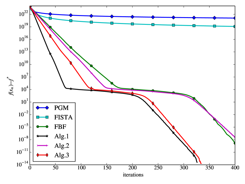
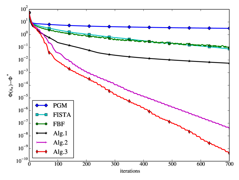
Figure 1: Results for problems (54) (left) and (55) (right)

	Constrained minimization (54)					Geometric programming (55)
	#iter	#$f$	#grad	#prox	time	#iter	#$f$	#grad	#prox	time
PGM	400	553	553	553	0.04	700	720	720	720	0.14
FISTA	400	953	553	553	0.06	700	1420	720	720	0.14
FBF	400	0	1446	1045	0.06	700	0	2746	2045	0.20
Alg.1	400	0	608	400	0.04	700	0	708	700	0.10
Alg.2	400	0	700	400	0.04	700	0	1472	700	0.13
Alg.3	400	0	626	400	0.04	700	0	1293	700	0.13

Table 1: Results for problems (54) and (55)

In fact, for this particular problem FBF and our proposed methods are almost equal regarding a speed of convergence. With different input data each of the fore-mentioned algorithms might show the best performance. However, our algorithms require much less evaluation.

Geometric programming

We consider a canonical example of geometric programming [6] for which we add $l_{1}$–norm:

$$\min_{x\in\mathbb{R}^{d}}\Phi(x):=\sum_{i=1}^{m}e^{\left\langle a_{i},x\right\rangle+b_{i}}+\left\langle c,x\right\rangle+\left\|x\right\|_{1},$$ (55)

where $a_{i},c\in\mathbb{R}^{d}$, $b\in\mathbb{R}^{m}$. Obviously, (55) is a particular case of (2) with

$$f(x)=\sum_{i=1}^{m}e^{\left\langle a_{i},x\right\rangle+b_{i}}+\left\langle c,x\right\rangle,\quad g(x)=\left\|x\right\|_{1}.$$

Clearly, $\nabla f(x)$ is not Lipschitz-continuous. We took $d=100$, $m=50$ and generated data $a_{i}$, $b$ and $c$ uniformly randomly from $(0,1)^{d}$, $(-1,1)^{m}$, and $(-1,1)^{d}$ respectively. The starting point was chosen as $x_{0}=(0,\dots,0)$. The results are presented on Fig. 1 and in Table 1.

Alg.1 shows the worst performance among proposed methods. In fact, there is no theoretical guarantee for its convergence for this problem. FBF with $\delta=2$ behaves similarly to FISTA and requires too much evaluation in contrast with our methods. However, FBF with $\delta=1$ behaved even worse as it almost coincided with PGM.

Analytic center

Suppose that set $C$ is a solution set of the following system of convex inequalities

$$f_{i}(x)\leq 0,\quad i=1,\dots,m.$$

The analytic center of the $C$ is defined as an optimal point of the problem

$$\min_{x\in\mathbb{R}^{d}}\sum_{i=1}^{m}-\log(-f_{i}(x))$$ (56)

This is a convex unconstrained minimization problem that is an instance of (2) with $g(x)=0$. However, in general $\nabla f$ is not Lipschitz-continuous.

In our experiment we seek the analytic center of $C$ that is defined as a polyhedron. In other words, we set $f_{i}(x)=\left\langle a_{i},x\right\rangle-b_{i}$ for $i=1,\dots,m$, where $a_{i}\in\mathbb{R}^{d}$, $b_{i}\in\mathbb{R}$. For a particular example we took $d=100$, $m=1000$, and generated $a_{i}$ uniformly randomly from $[-1,1]^{d}$. First $100$ coordinates of $b$ we set to $0.01$, the rest to $100$. On the one hand, this guarantees that $x_{0}=(0,\dots,0)$ belongs to $C$. And on the other hand, this makes $x_{0}$ close to some vertex of $C$ and hence, probably far from the analytic center. Because of this choice, $\nabla f$ changes very fast and PGM and FISTA do not give satisfactory results. The results are presented on Fig. 2 and in Table 2. Since this is an unconstrained problem, we ran Alg.1 using Remark 3.

Similarly to the previous problem, FBF with $\delta=2$ requires too much evaluation but with $\delta=1$ its performance was quite poor (the same as FISTA and PGM).

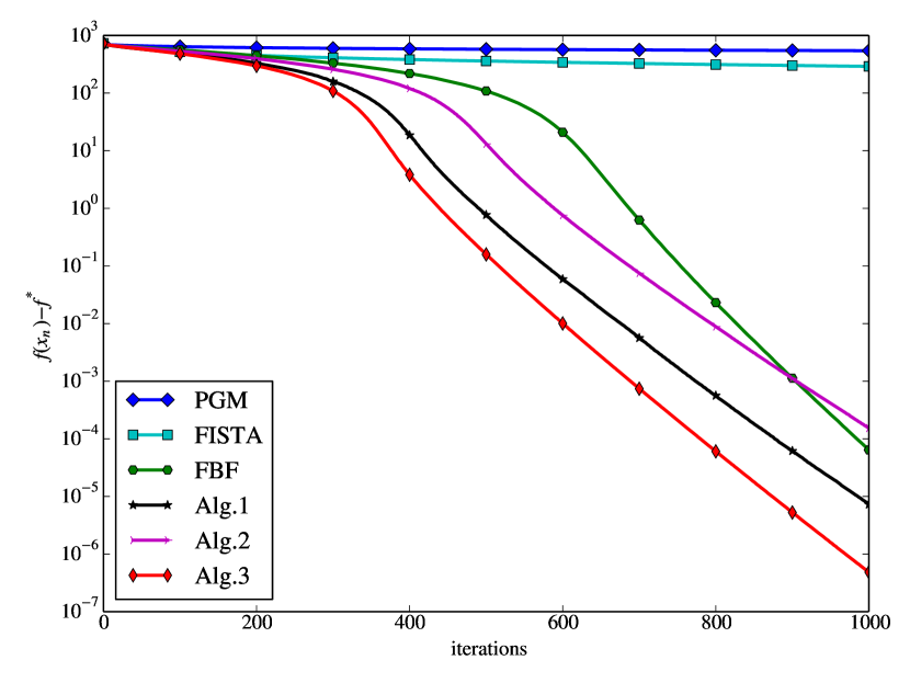
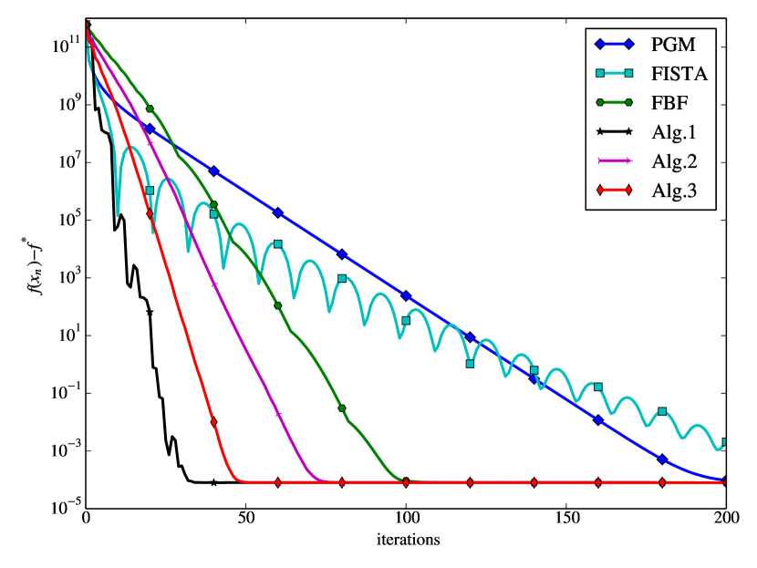
Figure 2: Results for problems (56) (left) and (57) (right)

	Analytic center (56)					$l_{p}$–minimization (57)
	#iter	#$f$	#grad	#prox	time	#iter	#$f$	#grad	#prox	time
PGM	1000	1044	1044	1044	0.96	200	235	235	235	0.04
FISTA	1000	2044	1044	1044	1.31	200	435	235	235	0.06
FBF	1000	0	3908	2907	1.83	200	0	784	583	0.06
Alg. 1	1000	0	1456	1000	0.89	200	0	312	200	0.04
Alg. 2	1000	0	1968	1000	1.11	200	0	405	200	0.04
Alg. 3	1000	0	1769	1000	1.08	200	0	369	200	0.04

Table 2: Results for problems (56) and (57)

$l_{p}$–minimization

Consider a problem of $l_{p}$–minimization

$$\min_{x\in\mathbb{R}^{d}}f(x)=\frac{1}{p}\sum_{i=1}^{m}\left\|x-a_{i}\right\|^{p},$$ (57)

where $a_{i}\in\mathbb{R}^{d}$. It is clear that for $p\geq 2$ (57) is an instance of (2). For a particular case $p=2$ this a well-known Fermat-Weber problem. We are interested in case when $p>2$ because this choice makes $\nabla f$ nonlinear. For a numerical experiment we choose $d=50$, $m=50$, $p=3$ and generated points $a_{i}$ uniformly randomly from $[-100,100]^{d}$. the starting points $x_{0}$ was chosen uniformly randomly from $[-1000,1000]^{d}$. Although it is clear that a solution of (57) belongs to the convex hull of $(a_{i})$, we intentionally choose $x_{0}$ as a random point from the larger range in order to make the problem harder. The results are presented on Fig. 2 and in Table 2. As previously, this is an unconstrained problem, so we ran Alg.1 with Remark 3.

Sun’s problem

Now consider a variational inequality that is not an instance of the optimization problem. We study a nonlinear VI, proposed by Sun [46]

$$\left\langle F(x^{*}),x-x^{*}\right\rangle\geq 0\quad\forall x\in C,$$ (58)

where

$$F(x) =F_{1}(x)+F_{2}(x),$$

$$F_{1}(x) =(f_{1}(x),f_{2}(x),\dots,f_{d}(x)),$$

$$F_{2}(x) =Dx+c,$$

$$f_{i}(x) =x_{i-1}^{2}+x_{i}^{2}+x_{i-1}x_{i}+x_{i}x_{i+1},\quad i=1,2,\dots,d,$$

$$x_{0} =x_{d+1}=0,$$

Here $D$ is a square matrix $d\times d$ defined by condition

$$d_{ij}=\begin{cases}4,&i=j,\\ 1,&i-j=1,\\ -2,&i-j=-1,\\ 0,&\text{otherwise},\end{cases}$$

and $c=(-1,-1,\dots,-1)$. We defined the feasible set as $C=[0,100]^{d}$. In the experiment we took $d=1000$ and the starting point was chosen uniformly randomly from $C$. We ran two variants of Tseng’s method with $\delta=1$ (TBF-1) and $\delta=2$ (TBF-2). For the comparison we used the residual $||x_{n}-P_{C}(x_{n}-F(x_{n}))||$. The results are presented on Fig. 3 and in Table 3.

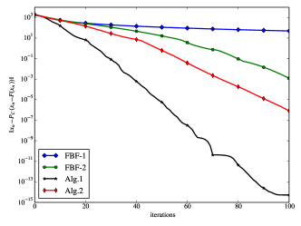
Figure 3: Results for problem (58)

	#iter	# $F$	#prox	time
FBF-1	100	201	100	30.6
FBF-2	100	384	283	52.8
Alg. 1	100	228	100	37.7
Alg. 2	100	191	100	30.9

Table 3: Results for problem (58)

Matrix game

We are interested in the following min-max matrix game

$$\min_{x\in\Delta_{l}}\max_{y\in\Delta_{k}}\left\langle Ax,y\right\rangle,$$ (59)

where $x\in\mathbb{R}^{l}$, $y\in\mathbb{R}^{k}$, $A\in\mathbb{R}^{k\times l}$, and $\Delta_{k}$, $\Delta_{l}$ denote the standard unit simplices in $\mathbb{R}^{k}$ and $\mathbb{R}^{l}$ respectively. The problem (59) is equivalent to the following variational inequality

$$\left\langle F(z^{*}),z-z^{*}\right\rangle+g(z)-g(z^{*})\geq 0$$

with

$$z=\binom{x}{y},\quad F(z)=\binom{A^{T}y}{-Ax},\quad g(z)=\binom{P_{\Delta_{l}}x}{P_{\Delta_{k}}y}.$$

As one can see, operator $F$ is linear, so we can run our methods Alg.1 and Alg.2 using Remark 2. In addition to FBF, we compared our methods with the primal-dual algorithm of Chambolle and Pock (PD). For that method we used fixed stepsizes $\tau=\sigma=\frac{1}{||A||}$ (as in paper [9]). In our experiment we took $k=1000$, $l=2000$ and generated two instances of matrix $A$ with entries (a) uniformly distributed and (b) normally distributed in $[-1,1]$.

The starting point for both cases was chosen as $x_{0}=\frac{1}{k}(1,\dots,1)$ and $y_{0}=\frac{1}{l}(1,\dots,1)$. In order to compute projection onto the unit simplex we used the algorithm from [17]. For a comparison we used a primal-dual gap $\mathcal{G}(x,y)$ which can be easily computed for a feasible pair $(x,y)$

$$\mathcal{G}(x,y)=\max_{i}(Ax)_{i}-\min_{j}(A^{T}y)_{j}.$$

Since iterates obtained by Tseng’s method may be infeasible, for a computation of primal-dual gap in this case we used the auxiliary point $z$ that is obtained by linesearch (see Section 4). As in the previous example, we ran two variants of FBF with $\delta=1$ and $\delta=2$. For this problem, instead of $\#F$, we counted the number of matrix-vector multiplication $\#\text{mult}$. Two projections onto simplices $\Delta_{k}$ and $\Delta_{l}$ respectively we counted as one prox.

When entries of $A$ were uniformly distributed, all algorithms behaved almost equally. Regarding the cost of one iteration, FBF methods are more expensive than other algorithms. Although the performance of PD, Alg.1, and Alg.2 was the same, the former extremely depends on the value of $||A||_{2}$. It ran much slower when we used $||A||_{F}$ instead of $||A||_{2}$. But in case of a huge scale problem evaluating of $||A||_{2}$ will be also quite resource-intensive.

When entries of $A$ were normally distributed, Alg.2 showed much better performance. And in both cases our algorithms required the same amount of computation as PD method. It is important to note that using FBF for this problem with $\delta=2$ makes the things only worse: it gives almost nothing for the speed of convergence and instead uses much more computational resources.

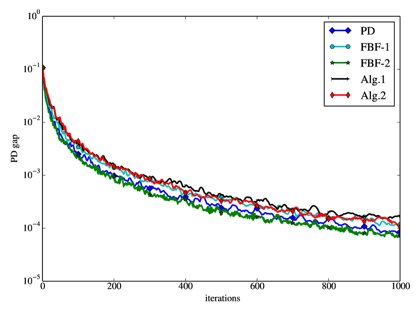
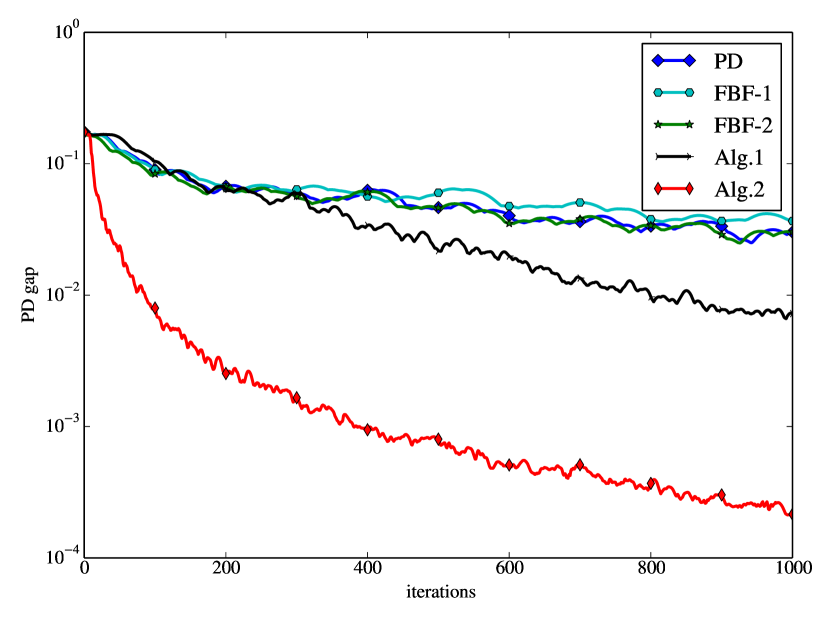
Figure 4: Results for problem (59): uniform case (left) and normal case (right)

	Uniform				Normal
	#iter	#mult	#prox	time	#iter	#mult	#prox	time
PD	1000	2000	1000	53.0	1000	2000	1000	53.3
FBF-1	1000	4006	1002	77.3	1000	4004	1001	78.2
FBF-2	1000	7892	2945	129.4	1000	7888	2943	128.4
Alg. 1	1000	2004	1000	51.9	1000	2004	1000	51.8
Alg. 2	1000	2004	1000	52.6	1000	2004	1000	52.7

Table 4: Results for problems (59)

5 Conclusion

In this paper there were proposed several algorithms for a general monotone variational inequality and a composite minimization problem. All methods use some simple linesearch procedure that allow to incorporate a local information of the operator. For all methods there was established the ergodic rate of convergence. Numerical experiments also approved their efficiency. Namely, we show that our methods can outperform proximal gradient method or FISTA with standard linesearch. Quite interesting is that the proposed methods become extremely simple when the operator is affine. In particular, for a minimax problem this makes the cost of one iteration the same as in the primal-dual algorithm and, on the other hand, may allow to use larger stepsizes. The requirement only of local Lipschitz-continuity of the operator makes our methods very general.

As numerical simulations showed, the ratio $\#F/\#\text{iter}$ (number of evaluation of the operator to the number of iterations) is almost always less than $2$. In the same time, this ratio for the extragradient method or forward-backward-forward method equals $2$ even when they do not use any linesearch. Moreover, the ratio $\#\text{prox}/\#\text{iter}$ for our methods always equals $1$.

The main drawback of the proposed methods is that we need the bound $\alpha=\sqrt{2}-1$. This multiplier makes the steps smaller in case when the Lipschitz constant of the operator does not change too much. It is interesting to study whether this bound can be increased.

Acknowledgement: The author acknowledges support from the Austrian science fund (FWF) under the project "Efficient Algorithms for Nonsmooth Optimization in Imaging" (EANOI) No. I1148.

References

- [1] J. Barzilai and J. M. Borwein, Two-point step size gradient methods, IMA Journal of Numerical Analysis, 8 (1988), pp. 141–148.
- [2] H. H. Bauschke and P. L. Combettes, Convex Analysis and Monotone Operator Theory in Hilbert Spaces, Springer, New York, 2011.
- [3] A. Beck and M. Teboulle, A fast iterative shrinkage-thresholding algorithm for linear inverse problem, SIAM Journal on Imaging Sciences, 2 (2009), pp. 183–202.
- [4] E. G. Birgin, J. M. Martínez, and M. Raydan, Nonmonotone spectral projected gradient methods on convex sets, SIAM Journal on Optimization, 10 (2000), pp. 1196–1211.
- [5] J. M. Borwein and Q. J. Zhu, Techniques of Variational Analysis, Springer, 2005.
- [6] S. Boyd and L. Vandenberghe, Convex Optimization, Cambridge University Press, 2004.
- [7] Y. Censor, A. Gibali, and S. Reich, The subgradient extragradient method for solving variational inequalities in Hilbert space, Journal of Optitmization Theory and Applications, 148 (2011), pp. 318–335.
- [8] A. Chambolle and T. Pock, A first-order primal-dual algorithm for convex problems with applications to imaging, Journal of Mathematical Imaging and Vision, 40 (2011), pp. 120–145.
- [9] , On the ergodic convergence rates of a first-order primal–dual algorithm, Mathematical Programming (to appear), (2015), pp. 1–35.
- [10] G. Cohen, Auxiliary problem principle extended to variational inequalities, Journal of Optimization Theory and Applications, 59 (1988), pp. 325–333.
- [11] P. L. Combettes and J.-C. Pesquet, A proximal decomposition method for solving convex variational inverse problems, Inverse problems, 24 (2008).
- [12] P. L. Combettes and J.-C. Pesquet, Proximal splitting methods in signal processing, in Fixed-Point Algorithms for Inverse Problems in Science and Engineering, H. H. Bauschke, R. S. Burachik, P. L. Combettes, V. Elser, D. R. Luke, and H. Wolkowicz, eds., Springer Optimization and Its Applications, Springer New York, 2011, pp. 185–212.
- [13] J. B. Cruz and T. Nghia, On the convergence of the proximal forward-backward splitting method with linesearches, arXiv:1501.02501, (2015).
- [14] S. Denisov, V. Semenov, and L. Chabak, Convergence of the modified extragradient method for variational inequalities with non-Lipschitz operators, Cybernetics and Systems Analysis, 51 (2015), pp. 757–765.
- [15] Q. T. Dinh, A. Kyrillidis, and V. Cevher, An inexact proximal path-following algorithm for constrained convex minimization, SIAM Journal on Optimization, 24 (2014), pp. 1718–1745.
- [16] , Composite self-concordant minimization, Journal of Machine Learning Research, 16 (2015), pp. 371–416.
- [17] J. Duchi, S. Shalev-Shwartz, Y. Singer, and T. Chandra, Efficient projections onto the l 1-ball for learning in high dimensions, in Proceedings of the 25th international conference on Machine learning, 2008, pp. 272–279.
- [18] I. Ekeland and R. Temam, Convex Analysis and Variational Problems, North-Holland, Amsterdam, Holland, 1976.
- [19] F. Facchinei and J.-S. Pang, Finite-Dimensional Variational Inequalities and Complementarity Problems, Volume I and Volume II, Springer-Verlag, New York, USA, 2003.
- [20] A. Gibali, A new non-Lipschitzian projection method for solving variational inequalities in Euclidean spaces, Journal of Nonlinear Analysis and Optimization, 6 (2015), pp. 41–51.
- [21] P. T. Harker and J.-S. Pang, Finite-dimensional variational inequality and nonlinear complementarity problems: A survey of theory, algorithms and applications, Mathematical Programming, 48 (1990), pp. 161–220.
- [22] A. N. Iusem and B. F. Svaiter, A variant of Korpelevich’s method for variational inequalities with a new search strategy, Optimization, 42 (1997), pp. 309–321.
- [23] E. N. Khobotov, Modification of the extragradient method for solving variational inequalities and certain optimization problems, USSR Computational Mathematics and Mathematical Physics, 27 (1989), pp. 120–127.
- [24] I. V. Konnov, Equilibrium models and variational inequalities, Elsevier, Amsterdam, 2007.
- [25] G. M. Korpelevich, The extragradient method for finding saddle points and other problems, Ekonomika i Matematicheskie Metody, 12 (1976), pp. 747–756.
- [26] Q. Lin and L. Xiao, An adaptive accelerated proximal gradient method and its homotopy continuation for sparse optimization, Computational Optimization and Applications, (2014), pp. 663–674.
- [27] P. L. Lions and B. Mercier, Splitting algorithms for the sum of two nonlinear operators, SIAM Journal on Numerical Analysis, 16 (1979), pp. 964–979.
- [28] D. Lorenz and T. Pock, An inertial forward-backward algorithm for monotone inclusions, Journal of Mathematical Imaging and Vision, 51 (2015), pp. 311–325.
- [29] S. I. Lyashko, V. V. Semenov, and T. A. Voitova, Low-cost modification of Korpelevich’s method for monotone equilibrium problems, Cybernetics and Systems Analysis, 47 (2011), pp. 631–639.
- [30] Y. Malitsky, Reflected projected gradient method for solving monotone variational inequalities, SIAM Journal on Optimization, 25 (2015), pp. 502–520.
- [31] Y. Malitsky and V. Semenov, A hybrid method without extrapolation step for solving variational inequality problems, Journal of Global Optimization, 61 (2015), pp. 193–202.
- [32] Y. V. Malitsky and V. V. Semenov, An extragradient algorithm for monotone variational inequalities, Cybernetics and Systems Analysis, 50 (2014), pp. 271–277.
- [33] A. Moudafi and M. Oliny, Convergence of a splitting inertial proximal method for monotone operators, Journal of Computational and Applied Mathematics, 155 (2003), pp. 447–454.
- [34] A. Nemirovski, Prox-method with rate of convergence for variational inequalities with Lipschitz continuous monotone operators and smooth convex-concave saddle point problems, SIAM Journal on Optimization, 15 (2004), pp. 229–251.
- [35] Y. Nesterov, A method of solving a convex programming problem with convergence rate , Soviet Mathematics Doklady, 27 (1983), pp. 372–376.
- [36] , Gradient methods for minimizing composite objective function, CORE discussion paper 2007076, Université Catholique de Louvain, Center for Operations Research and Econometrics, (2007).
- [37] B. O’Donoghue and E. Candes, Adaptive restart for accelerated gradient schemes, Foundations of computational mathematics, (2013), pp. 1–18.
- [38] N. Parikh and S. Boyd, Proximal algorithms, Foundations and Trends in Optimization, 1 (2014).
- [39] G. B. Passty, Ergodic convergence to a zero of the sum of monotone operators in Hilbert space, J. Math. Anal. Appl, (1979), pp. 383–390.
- [40] B. Polyak, Some methods of speeding up the convergence of iteration methods., U.S.S.R. Computational Mathematics and Mathematical Physics, 4 (1967), pp. 1–17.
- [41] L. D. Popov, A modification of the Arrow-Hurwicz method for finding saddle points, Mathematical Notes, 28 (1980), pp. 845–848.
- [42] N. Pustelnik, J.-C. Pesquet, and C. Chaux, Proximal methods for image restoration using a class of non-tight frame representations, in Proc. Eur. Sig. and Image Proc. Conf. Aalborg, Danmark, 2010.
- [43] K. Scheinberg, D. Goldfarb, and X. Bai, Fast first-order methods for composite convex optimization with backtracking, Foundations of Computational Mathematics, 14 (2014), pp. 389–417.
- [44] M. V. Solodov and B. F. Svaiter, A new projection method for variational inequality problems, SIAM Journal on Control and Optimization, 37 (1999), pp. 765–776.
- [45] M. V. Solodov and P. Tseng, Modified projection-type methods for monotone variational inequalities, SIAM Journal on Control and Optimization, 34 (1996), pp. 1814–1830.
- [46] D. Sun, A projection and contraction method for the nonlinear complementarity problems and its extensions, Mathematica Numerica Sinica, 16 (1994), pp. 183–194.
- [47] P. Tseng, A modified forward-backward splitting method for maximal monotone mappings, SIAM Journal on Control and Optimization, 38 (2000), pp. 431–446.
- [48] , On accelerated proximal gradient methods for convex-concave optimization, 2008.