Exact solutions to plaquette Ising models with free and periodic boundaries

Abstract

An anisotropic limit of the $3d$ plaquette Ising model, in which the plaquette couplings in one direction were set to zero, was solved for free boundary conditions by Suzuki (Phys. Rev. Lett. 28 (1972) 507), who later dubbed it the fuki-nuke, or “no-ceiling”, model. Defining new spin variables as the product of nearest-neighbour spins transforms the Hamiltonian into that of a stack of (standard) $2d$ Ising models and reveals the planar nature of the magnetic order, which is also present in the fully isotropic $3d$ plaquette model. More recently, the solution of the fuki-nuke model was discussed for periodic boundary conditions, which require a different approach to defining the product spin transformation, by Castelnovo et al. (Phys. Rev. B 81 (2010) 184303).

We clarify the exact relation between partition functions with free and periodic boundary conditions expressed in terms of original and product spin variables for the $2d$ plaquette and $3d$ fuki-nuke models, noting that the differences are already present in the $1d$ Ising model. In addition, we solve the $2d$ plaquette Ising model with helical boundary conditions. The various exactly solved examples illustrate how correlations can be induced in finite systems as a consequence of the choice of boundary conditions.

1 Introduction

The strongly anisotropic limit of a purely plaquette Ising Hamiltonian on a $3d$ cubic lattice

$$\mathcal{H}=-J\sum_{\Box}\sigma\sigma\sigma\sigma\;,$$ (1)

where we denote the product of the spins sited at vertices around a plaquette by $\Box$ and in which the plaquette coupling $J$ in one direction is set to zero, may be solved exactly [1, 2]. A variable transformation in which a product of nearest-neighbour spins in the direction perpendicular to the non-contributing plaquettes is made, $\hat{\tau}_{i}=\sigma_{i-1}\sigma_{i}$, reveals that the model (later dubbed fuki-nuke by Hashizume and Suzuki [3]) is non-trivially equivalent to a stack of standard $2d$ Ising models with nearest-neighbour pair interactions in each plane.

The nature of the order in the fuki-nuke model is rather unusual since the $\tau$-spins may magnetize independently in each $2d$ Ising plane. In terms of the original $\sigma$ spins this order is encoded in nearest-neighbour correlators perpendicular to the direction in which the plaquette coupling is zero. An isotropic version of this planar order exists for the isotropic plaquette Hamiltonian [3, 4]. The isotropic model in Eq. (1) has a strong first-order phase transition [5] with several interesting properties itself. It displays non-standard finite-size scaling because of its exponentially degenerate low-temperature phase [6] and it also has glassy characteristics [7], in spite of the absence of any quenched disorder. It can also be thought of as a particular limit of a family of gonihedric [8, 9] Ising models containing nearest-neighbour, next-to-nearest-neighbour and plaquette interactions tuned to remove the bare area contribution of (geometric) spin clusters.

Suzuki’s original solution of the fuki-nuke model employed free boundary conditions [1], whereas periodic boundary conditions, as often used in numerical simulations, were considered in [2]. Although the treatment of the product variable transformation $\hat{\tau}_{i}=\sigma_{i-1}\sigma_{i}$ in the two cases can, loosely, be argued to be identical in the thermodynamic limit as a post-hoc justification for ignoring any subtleties, it is possible to treat the variable transformation for both free and periodic boundary conditions in the fuki-nuke model exactly and we shall do so here. Since such differences arising from boundary conditions may impact the finite-size scaling properties in simulations, careful consideration of both cases is worthwhile.

Interestingly, the differences arising in using the product variable transformation for free and periodic boundary conditions are already present for the nearest-neighbour $1d$ Ising model. While the product spin transformation has been widely used to obtain the solution of the $1d$ Ising model for free boundary conditions, the discussion of periodic boundaries where constraints must be imposed on the allowed spin configurations is less well known and the differences between the two are pointed out in preparation of similar calculations in the $2d$ plaquette and $3d$ fuki-nuke models in Sec. 2, which also serves as a reference when expressing the solutions to the more complicated models in terms of $1d$ Ising partition functions.

In Sec. 3, we investigate the finite-size behaviour of the $2d$ plaquette Ising model, which appears as a different anisotropic limit of the $3d$ plaquette Ising model using the product spin approach. The exact solution of the $2d$ plaquette Ising model illustrates clearly how non-trivial correlations can enter finite systems as a consequence of the choice of the boundary conditions

In Sec. 4, we discuss the $3d$ anisotropic, fuki-nuke model itself, following closely the $1d$ Ising template, since the technical issues are similar. As with the $2d$ plaquette model, periodic boundary conditions are found to induce correlations in the finite-size fuki-nuke model in comparison to the (simpler) case of free boundaries. Along the way we present an exact numerical enumeration of the partition function, confirming the equality of the expressions in terms of the original, $\sigma$, and product, $\tau$, spins in the case of the fuki-nuke model. Finally, Sec. 5 contains our conclusions.

2 One Dimension: The Standard $1d$ Ising Model

The $1d$ Ising model provides perhaps the standard pedagogical example of an exactly solvable model in statistical mechanics, albeit one without a phase transition at finite temperature, as Ising himself discovered [11] to his disappointment. It is often discussed using periodic boundary conditions and a transfer matrix approach, since this allows a straightforward solution, even in non-zero external field. With a view to the solution of the fuki-nuke model we consider the model in zero external field and take a different approach, in effect changing the variables in the partition function so that it takes a factorized form and may be evaluated trivially. The steps required to do this differ for the case of free and periodic boundary conditions and we deal with each separately.

2.1 Free Boundary Conditions

If we consider the standard nearest-neighbour Ising Hamiltonian with spins $\sigma_{i}=\pm 1$ on a linear chain of length $L$ in one dimension

$$H=-\sum_{i=1}^{L-1}\sigma_{i}\sigma_{i+1}$$ (2)

with free boundary conditions, then the partition function

$$Z_{1d,\;{\rm free}}=\sum_{\{\sigma\}}\exp\left(\beta\sum_{i=1}^{L-1}\sigma_{i}\sigma_{i+1}\right)$$ (3)

may be evaluated by defining the variable transformation

$$\{\sigma_{1},\sigma_{2},\ldots\sigma_{L}\}\rightarrow\{\tau_{1},\tau_{2},\ldots\tau_{L}\}\;,$$ (4)

where $\tau_{1}=\sigma_{1}\sigma_{2},\,\tau_{2}=\sigma_{2}\sigma_{3},\,\ldots,\tau_{L-1}=\sigma_{L-1}\sigma_{L}$. Setting $\tau_{L}=\sigma_{L}$ the mapping $\{\sigma\}\rightarrow\{\tau\}$ with an inverse relation of the form $\sigma_{i}=\tau_{L}\,\tau_{L-1}\,\tau_{L-2}\cdots\tau_{i}$ is one-to-one. This allows us to write $Z$ in factorized form as

$$Z_{1d,\;{\rm free}}=\sum_{\{\tau\}}\exp\left(\beta\sum_{i=1}^{L-1}\tau_{i}\right)$$ (5)

which may then trivially be evaluated to give

$$Z_{1d,\;{\rm free}}=2\prod_{i=1}^{L-1}\sum_{\tau_{i}=\pm 1}\exp\left(\beta\tau_{i}\right)=2(2\operatorname{ch}(\beta))^{L-1}$$ (6)

where the initial factor of two comes from the sum over $\tau_{L}=\sigma_{L}$ which does not appear in the exponent. We highlight two features of this calculation, which also appear when the transformation is applied to the fuki-nuke model with free boundaries:

• The last spin, $\sigma_{L}$, remains untransformed,

• summing over this gives a factor of $2$ in $Z_{1d,\;{\rm free}}$.

2.2 Periodic Boundary Conditions

When periodic boundary conditions are imposed, we map $L$ $\sigma$’s to $L$ $\tau$’s without requiring the condition $\tau_{L}=\sigma_{L}$ of the free boundary conditions. Since every configuration of $\tau$’s can now be made up from two configurations of $\sigma$’s, this should be taken into account when relating the partition functions expressed in terms of $\sigma$ or $\tau$. Explicitly, the transformations are now given by $\tau_{1}=\sigma_{1}\sigma_{2},\,\tau_{2}=\sigma_{2}\sigma_{3},\,\ldots,\tau_{L}=\sigma_{L}\sigma_{L+1}=\sigma_{L}\sigma_{1}$, with an inverse relation of the form $\sigma_{i}=\sigma_{1}\times\tau_{1}\,\tau_{2}\,\tau_{3}\cdots\tau_{i-1}$, and a direct consequence of the periodic boundary conditions is that the constraint

$$\prod_{i=1}^{L}\tau_{i}=\prod_{i=1}^{L}\sigma_{i}^{2}=1$$ (7)

must be imposed on the $\tau$-variables. This can be implemented in the partition function as

$$Z_{1d,\;{\rm periodic}}=2\sum_{\{\tau\}}\exp\left(\beta\sum_{i=1}^{L}\tau_{i}\right)\delta\left(\prod_{i=1}^{L}\tau_{i},1\right)\;,$$ (8)

where the requisite factor of two takes account of the two-to-one $\sigma$-to-$\tau$-mapping. Since $\prod_{i=1}^{L}\tau_{i}=\pm 1$, it is possible to rewrite the Kronecker-$\delta$ function appearing in Eq. (8) as

$$Z_{1d,\;{\rm periodic}}=\sum_{\{\tau\}}\exp\left(\beta\sum_{i=1}^{L}\tau_{i}\right)\left(1+\prod_{i=1}^{L}\tau_{i}\right)\,$$ (9)

which subsumes the factor of two. The partition function written in this form may now be straightforwardly evaluated as the sum of two factorized terms,

$$Z_{1d,\;{\rm periodic}} = \left[\prod_{i=1}^{L}\sum_{\tau_{i}=\pm 1}\exp\left(\beta\tau_{i}\right)+\prod_{i=1}^{L}\sum_{\tau_{i}=\pm 1}\tau_{i}\exp\left(\beta\tau_{i}\right)\right]$$ (10)

$$= 2^{L}\left[\operatorname{ch}(\beta)^{L}+\operatorname{sh}(\beta)^{L}\right]$$

$$= 2^{L}\operatorname{ch}(\beta)^{L}\left[1+\operatorname{th}(\beta)^{L}\right]\;.$$

The standard result for periodic boundary conditions, familiar from the transfer matrix calculation and numerous other approaches, is hence recovered. In the case of periodic boundary conditions we can see that:

• The last spin, $\sigma_{L}$, is included in the transformation,

• an additional factor of two appears in order to ensure the equivalence of the $\sigma$- and $\tau$-representations of the partition function,

• a constraint must be imposed on the product of all the $\tau$-variables resulting in two terms in the partition function, corresponding to an additional correlation by comparison with free boundary conditions.

The factor of two thus appears for different reasons in the $\tau$-representation of the partition function in the free boundary case (summing over the last spin) and the periodic boundary case (a two-to-one mapping between $\sigma$’s and $\tau$’s).

3 Two Dimensions: The $2d$ Gonihedric Ising Model

Consider the anisotropic version of the Hamiltonian in Eq. (1),

$$H_{\rm aniso}(\{\sigma\}) = -J_{x}\sum_{x=1}^{L_{x}}\sum\limits_{y=1}^{L_{y}}\sum\limits_{z=1}^{L_{z}}\sigma_{x,y,z}\sigma_{x,y+1,z}\sigma_{x,y+1,z+1}\sigma_{x,y,z+1}$$

$$-J_{y}\sum_{x=1}^{L_{x}}\sum\limits_{y=1}^{L_{y}}\sum\limits_{z=1}^{L_{z}}\sigma_{x,y,z}\sigma_{x+1,y,z}\sigma_{x+1,y,z+1}\sigma_{x,y,z+1}$$

$$-J_{z}\sum_{x=1}^{L_{x}}\sum\limits_{y=1}^{L_{y}}\sum\limits_{z=1}^{L_{z}}\sigma_{x,y,z}\sigma_{x+1,y,z}\sigma_{x+1,y+1,z}\sigma_{x,y+1,z}\;,$$

where we have now indicated each site and directional sum explicitly. If we now set the coupling of the vertical plaquettes to zero, the different horizontal layers decouple trivially and the Hamiltonians of the individual layers are those of the two-dimensional plaquette (gonihedric) [8, 9] model,

$$H_{\rm aniso}^{J_{x}=J_{y}=0}(\{\sigma\})=-J_{z}\sum\limits_{z=1}^{L_{z}}\left[\;\sum_{2d\;\Box}\sigma\sigma\sigma\sigma\right]\;.$$ (12)

Taking $J_{z}=1$ for simplicity, the partition function is given by the product of $L_{z}$ decoupled layers,

$$Z_{\rm aniso}^{J_{x}=J_{y}=0}=\sum_{\{\sigma\}}\exp\left(-\beta H_{\rm aniso}^{J_{x}=J_{y}=0}(\{\sigma\})\right)=(Z_{2d,\;{\rm gonihedric}})^{L_{z}}\;,$$ (13)

each of which is a $2d$ plaquette model. The partition function for the $2d$ plaquette model may also be evaluated exactly using the spin-bond ($\sigma$-$\tau$)-transformation for both free and periodic boundary conditions in the direction of the transformation, which we shall take in in the following along the vertical $y$-axis.

3.1 Free Boundary Conditions in $y$-Direction

On a rectangular $L_{x}\times L_{y}$ lattice with free boundaries in the $y$-direction, the $\sigma$-$\tau$-transformation used in the $1d$ Ising model can still be applied in $y$-direction by defining $\tau_{x,y}=\sigma_{x,y}\sigma_{x,y+1}$, with the condition $\tau_{x,L_{y}}=\sigma_{x,L_{y}}$ and the inverse relation $\sigma_{x,y}=\tau_{x,L_{y}}\tau_{x,L_{y}-1}\cdots\tau_{x,y}$. Assuming free boundaries in $x$-direction, too, the partition function reads

$$Z_{2d,\;{\rm gonihedric},\;{\rm free}} = \sum_{\{\sigma\}}\exp\left(\beta\sum\limits_{x=1}^{L_{x}-1}\sum\limits_{y=1}^{L_{y}-1}\sigma_{x,y}\sigma_{x,y+1}\sigma_{x+1,y}\sigma_{x+1,y+1}\right)$$ (14)

$$= \sum_{\{\tau\}}\exp\left(\beta\sum\limits_{x=1}^{L_{x}-1}\sum\limits_{y=1}^{L_{y}-1}\tau_{x,y}\tau_{x+1,y}\right)$$

$$= 2^{L_{x}}(Z_{1d,\;{\rm Ising}})^{L_{y}-1}\;,$$

where the factor $2^{L_{x}}$ in the last line comes from the $L_{x}$ sums over $\tau_{x,L_{y}}=\sigma_{x,L_{x}}=\pm 1$ which do not appear in the exponent, similar to the $1d$ Ising case. Products of the partition function of the $1d$ Ising model appear due to the decoupling in $\tau$-spins in the $y$-direction. The solution of the free $1d$ Ising model from Eq. (6) simplifies this expression to

$$Z_{2d,\;{\rm gonihedric},\;{\rm free,\;free}} = 2^{L_{x}L_{y}}\operatorname{ch}\left(\beta\right)^{(L_{x}-1)(L_{y}-1)}\;.$$ (15)

With periodic boundary conditions in $x$-direction, the partition function $Z_{1d,\;{\rm Ising}}$ in (14) is the solution (10) of the periodic case, so that the explicit expression looks slightly more complicated,

$$Z_{2d,\;{\rm gonihedric},\;{\rm periodic,\;free}}=2^{L_{x}L_{y}}\operatorname{ch}\left(\beta\right)^{L_{x}(L_{y}-1)}\left(1+\operatorname{th}\left(\beta\right)^{L_{x}}\right)^{L_{y}-1}$$

$$\qquad=2^{L_{x}L_{y}}\operatorname{ch}\left(\beta\right)^{L_{x}(L_{y}-1)}\sum_{h=0}^{L_{y}-1}{L_{y}-1\choose h}\operatorname{th}(\beta)^{L_{x}h}\;.$$ (16)

The expansion in the last line gives binomials of $\operatorname{th}(\beta)$, which also appear below when periodic boundaries in both directions are considered.

3.2 Periodic Boundary Conditions in $y$-Direction

To simplify the combinatorics involved when solving the model with periodic boundary conditions, we employ a dimer representation that allows us to straightforwardly take into account the constraints that arise with periodic boundaries. This diagrammatic approach appears naturally in the high-temperature representation as a way of representing valid configurations graphically.

If we take periodic boundary conditions in $y$-direction, i.e., $\sigma_{L_{x}+1,y}=\sigma_{1,y}$ and $\sigma_{x,L_{y}+1}=\sigma_{x,1}$, the transformation $\tau_{x,y}=\sigma_{x,y}\sigma_{x,y+1}$ imposes the $L_{x}$ constraints $\prod_{y}\tau_{x,y}=1$ and leads to an inverse relation of the form

$$\sigma_{x,y}=\sigma_{x,1}\times\tau_{x,1}\,\tau_{x,2}\,\tau_{x,3}\cdots\tau_{x,y-1}\;.$$ (17)

This allows the partition function to be expressed in terms of the new $\tau$-variables as

$$Z_{2d,\;{\rm gonihedric},\;{\rm periodic}}=\sum\limits_{\{\sigma\}}\exp\left(\beta\sum_{x=1}^{L_{x}}\sum_{y=1}^{L_{y}}\sigma_{x,y}\sigma_{x,y+1}\sigma_{x+1,y}\sigma_{x+1,y+1}\right)$$

$$\qquad=2^{L_{x}}\sum\limits_{\{\tau\}}\exp\left(\beta\sum_{x=1}^{L_{x}}\sum_{y=1}^{L_{y}}\tau_{x,y}\tau_{x+1,y}\right)\prod_{x=1}^{L_{x}}\delta\left(\prod_{y=1}^{L_{y}}\tau_{x,y},1\right)\;,$$ (18)

where the prefactor of $2^{L_{x}}$ again accounts for the two-to-one $\sigma$-to-$\tau$-mapping. The notation in Eq. (3.2) assumes periodic boundary conditions also in $x$-direction, although this is not essential for what follows (for free boundary conditions we would have the replacement, $\sum_{x=1}^{L_{x}}\rightarrow\sum_{x=1}^{L_{x}-1}$).

This can be rewritten in the high-temperature representation as an expression which looks similar to the starting point of the combinatorial solution of the standard $2d$ Ising model [13],

$$\qquad Z_{2d,\;{\rm gonihedric},\;{\rm periodic}} =$$ (19)

$$\qquad 2^{L_{x}}\operatorname{ch}(\beta)^{L_{x}L_{y}}\sum\limits_{\{\tau\}} \left[\,\prod_{y=1}^{L_{y}}\prod_{x=1}^{L_{x}}\left(1+\operatorname{th}\left(\beta\right)\tau_{x,y}\tau_{x+1,y}\right)\right]\prod_{x=1}^{L_{x}}\delta\left(\prod_{y=1}^{L_{y}}\tau_{x,y},1\right).$$

Here, however, we are saved from the combinatorial complications of counting loops because the spins only couple in the $x$ (horizontal) direction in our case. Graphically the factors of $\operatorname{th}(\beta)\tau_{x,y}\tau_{x+1,y}$, which appear when expanding the product in Eq. (19), are represented as horizontal dimers. This amounts to the diagrammatical solution of the $1d$ Ising model using the high-temperature representation, up to subtle complications due to the $\delta$-constraints discussed further below.

Let us first verify that, within this diagrammatic approach, the results of the preceding subsection in Eqs. (15) and (16) are immediately recovered: For the case with free boundaries in both directions, the $\delta$-constraints (and also the associated $2^{L_{x}}$ prefactor) are absent, so $1,\dots,(L_{x}-1)\times(L_{y}-1)$ dimers cannot be arranged without any dangling ends, since summing over the spins on the free dimer ends would give a zero contribution to the partition function. This leaves the empty lattice as the only contributing dimer configuration, giving the $2^{L_{x}L_{y}}$ factor in Eq. (15) from the then trivial summations over the $\tau$-spins. In the other case with free boundaries in $x$ (horizontal) direction, and periodic boundary conditions in $y$-direction, the direction in which the $\sigma$-$\tau$-transformation is carried out, the $L_{x}$ $\delta$-constraints couple the spins non-locally so that complete columns of dimers contribute, too. There are $L_{x}-1\choose v$ possible ways of choosing $v$ such columns, each one carrying a weight of $\operatorname{th}(\beta)^{L_{y}v}$. Summing over all possible numbers for $v$, the symmetric counterpart of Eq. (16) is recovered, with $L_{x}$ and $L_{y}$ swapped (since here the $\sigma$-$\tau$-transformation was carried out in the other direction). The prefactor $2^{L_{x}L_{y}}=2^{L_{x}}2^{L_{x}(L_{y}-1)}$ is the product of the factor $2^{L_{x}}$ in Eq. (19) and the weight of $2^{L_{x}(L_{y}-1)}$ for each diagram of dimers, which takes care of proper summation over all $\tau$-configurations. Here, for each of the $L_{x}$ spin columns (not to be confused with the $L_{x}-1$ dimer columns), the $L_{y}$ summations over $\tau_{x,y}$ give a trivial factor of $2$, except for one summation (say, the first) which gives only 1 due to summing over the $\delta$-constraint.

After these checks, we are ready to consider the doubly periodic case (i.e., the torus topology), where periodic boundary conditions are assumed in both $x$- and $y$-direction and the graphical representation is slightly more complicated. Here not only empty but also completely filled rows (“closed” by the periodic boundary conditions in $x$-direction) of dimers would normally contribute. However, due to the $\delta$-constraints, gaps in the otherwise filled rows of dimers may also be present. As a consequence, both a horizontal configuration of dimers and its “dual”, where shaded and unshaded bonds are swapped, may appear. In Fig. 1 a contributing configuration to the $L_{x}=L_{y}=6$ partition function is shown, where the dimers giving $\operatorname{th}(\beta)$ factors are shown heavily shaded. The two sorts of contributing horizontal lines give either an $\operatorname{th}(\beta)^{4}$ or $\operatorname{th}(\beta)^{2}$ factor in this case. In general on an $L_{x}\times L_{y}$ lattice there may be $v=0,...,L_{x}$ gaps in a shaded line which may be chosen in ${L_{x}\choose v}$ ways and counting these and their duals gives

$$\qquad Z_{2d,\;{\rm gonihedric},\;{\rm periodic}} =$$ (20)

$$\qquad\left(\frac{1}{2}\right) 2^{L_{x}L_{y}}\operatorname{ch}(\beta)^{L_{x}L_{y}}\sum\limits_{v=0}^{L_{x}}{L_{x}\choose v}\left(\operatorname{th}(\beta)^{v}+\operatorname{th}(\beta)^{L_{x}-v}\right)^{L_{y}}\,.$$

The prefactor of $1/2$ takes care of the double-counting inherent in the dimer description due to the $v\leftrightarrow L_{x}-v$ symmetry. The diagram of Fig. 1, for instance, appears in both the $v=2$ and $v=4$ terms in the sum of Eq. (20). The other prefactor, $2^{L_{x}L_{y}}=2^{L_{x}}2^{L_{x}(L_{y}-1)}$ results as above from the now trivial summations over the $\tau$-spins, respecting the $L_{x}$ $\delta$-constraints (which kill one of the factors of 2 for each of the $L_{x}$ spin columns).

Figure 1: A contributing dimer configuration in the $2d$ gonihedric case with periodic boundary conditions in both directions for $L_{x}=L_{y}=6$, combining both $\operatorname{th}(\beta)^{4}$ and $\operatorname{th}(\beta)^{2}$ terms.

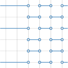
Expanding the product in Eq. (20) gives an alternative representation of the partition function as a double sum, which was also found by Espriu and Prats [14] for the special case $L_{x}=L_{y}=L$ by enumerating possible plaquette configurations. In this approach rows and columns of plaquettes which can contribute to the partition function sum are counted, keeping track of over-counting factors of $\operatorname{th}(\beta)$ in intersecting rows and columns:

$$\qquad Z_{2d,\;{\rm gonihedric},\;{\rm periodic}} =$$ (21)

$$\qquad\left(\frac{1}{2}\right) 2^{L_{x}L_{y}}\operatorname{ch}(\beta)^{L_{x}L_{y}}\sum\limits_{v=0}^{L_{x}}\sum_{h=0}^{L_{y}}{L_{x}\choose v}{L_{y}\choose h}\operatorname{th}(\beta)^{vL_{y}+hL_{x}-2vh}\;.$$

In A we show how enumerating plaquette configurations also allows the exact solution of the model with helical boundary conditions as considered recently in a numerical Monte Carlo simulation study [15].

In summary, although we have used the same transformation, the solution for the model with periodic boundary conditions can be seen to be more involved than the (almost) trivial free case in Sec. 3.1. This is a consequence of the constraints that implement the periodic boundary conditions, which couple the different $1d$ layers and allow non-trivial $1d$ configurations to contribute to the partition function sum. As we will now see, this behaviour is repeated in the three-dimensional fuki-nuke model where free boundary conditions lead to a partition function composed of uncoupled $2d$ layers, whereas periodic boundaries give a much more complicated structure.

4 Three Dimensions: The Fuki-Nuke Model

4.1 The Fuki-Nuke Model

The fuki-nuke model [1, 3] is the $J_{z}=0$ limit of the anisotropic $3d$ plaquette model defined in Eq. (3). In this case the horizontal, “ceiling” plaquettes have zero coupling, which Hashizume and Suzuki denoted the fuki-nuke (“no-ceiling” in Japanese) model [3]. The anisotropic $3d$ plaquette Hamiltonian when $J_{z}=0$ is thus given by

$$H_{\rm fuki\mathchar 45\relax nuke}(\{\sigma\}) = -J_{x}\sum_{x=1}^{L}\sum\limits_{y=1}^{L}\sum\limits_{z=1}^{L_{z}}\sigma_{x,y,z}\sigma_{x,y+1,z}\sigma_{x,y+1,z+1}\sigma_{x,y,z+1}$$ (22)

$$-J_{y}\sum_{x=1}^{L}\sum\limits_{y=1}^{L}\sum\limits_{z=1}^{L_{z}}\sigma_{x,y,z}\sigma_{x+1,y,z}\sigma_{x+1,y,z+1}\sigma_{x,y,z+1}\;,$$

with $L_{z}\geq 2$. This Hamiltonian, with $J_{x}=J_{y}=1$ for simplicity, may be solved for free boundary conditions in $z$-direction by using the same variable transformation as in the $1d$ Ising model. When expressed in terms of the new product spin variables $\tau$ the Hamiltonian for free boundary conditions can be seen to be that of a stack of $2d$ Ising models with nearest-neighbour in-plane interactions. The differences in the treatment of free and periodic boundary conditions that are manifest in the $1d$ model also appear here, so we treat each separately.

4.2 Free Boundary Conditions in $z$-Direction

For free boundary conditions in $z$-direction (the case originally discussed by Suzuki [1]) we define bond spin variables $\tau_{x,y,z}=\sigma_{x,y,z}\sigma_{x,y,z+1}$ on each vertical lattice bond in a cuboidal $L\times L\times L_{z}$ lattice. The $\sigma$- and $\tau$-spins are related by

$$\tau_{x,y,1}=\sigma_{x,y,1}\,\sigma_{x,y,2}\,,\,\ldots\,,\;\tau_{x,y,L_{z}-1}=\sigma_{x,y,L_{z}-1}\,\sigma_{x,y,L_{z}}\,,\;\tau_{x,y,L_{z}}=\sigma_{x,y,L_{z}}\;,$$ (23)

with an inverse relation of the form

$$\sigma_{x,y,z}=\tau_{x,y,L_{z}}\,\tau_{x,y,L_{z}-1}\,\tau_{x,y,L_{z}-2}\cdots\tau_{x,y,z}\;,$$ (24)

where a one-to-one correspondence between the $\sigma$- and $\tau$-spin configurations is maintained by specifying that the value of the $\sigma,\tau$-spins on a given horizontal plane (in this case $z=L_{z}$, i.e., $\tau_{x,y,L_{z}}=\sigma_{x,y,L_{z}}$) are equal. The resulting Hamiltonian is missing one layer of spins,

$$H_{\rm fuki\mathchar 45\relax nuke}(\{\tau\})=-\sum\limits_{x=1}^{L}\sum\limits_{y=1}^{L}\sum\limits_{z=1}^{L_{z}-1}\left(\tau_{x,y,z}\tau_{x+1,y,z}+\tau_{x,y,z}\tau_{x,y+1,z}\right)\;,$$ (25)

so summing over these gives an additional factor of $2^{L\times L}$ in the partition function (corresponding to the factor of $2$ in Eq. (6)),

$$Z_{\rm fuki\mathchar 45\relax nuke} = \sum_{\{\tau\}}\exp\left(-\beta H_{\rm fuki\mathchar 45\relax nuke}(\{\tau\})\right)$$ (26)

$$= 2^{L^{2}}\sum_{\{\tau_{x,y,z\neq L_{z}}\}}\prod_{z=1}^{L_{z}-1}\exp\left(\beta\sum\limits_{x=1}^{L}\sum\limits_{y=1}^{L}\left(\tau_{x,y,z}\tau_{x+1,y,z}+\tau_{x,y,z}\tau_{x,y+1,z}\right)\right)$$

$$= 2^{L^{2}}\prod_{z=1}^{L_{z}-1}\sum_{\{\tau_{x,y}\}_{z}}\exp\left(\beta\sum\limits_{x=1}^{L}\sum\limits_{y=1}^{L}\left(\tau_{x,y,z}\tau_{x+1,y,z}+\tau_{x,y,z}\tau_{x,y+1,z}\right)\right)$$

$$= 2^{L^{2}}\prod_{z=1}^{L_{z}-1}Z_{2d\;\rm Ising}=2^{L^{2}}\left(Z_{2d\;\rm Ising}\right)^{L_{z}-1},$$

where $\{\tau_{x,y}\}_{z}$ denotes summation over all $\tau$-spins with a given $z$-component and $Z_{2d\;\rm Ising}$ is the standard partition function of the $2d$ Ising layer. The boundary conditions in $x$- and $y$-directions are arbitrary, as long as boundaries of different layers are not coupled, i.e., boundary conditions have no dependence on $z$ (the explicit notation in Eqs. (25) and (26) assumes periodic boundary conditions, but other conditions would carry through the calculation, too). By taking the limit of infinite layers (but keeping $L_{z}$ fixed), one easily arrives at

$$\beta f_{\rm fuki\mathchar 45\relax nuke}\equiv-\lim_{L\rightarrow\infty}\frac{1}{L^{2}L_{z}}\ln Z_{\rm fuki\mathchar 45\relax nuke}=\beta f_{2d\;\rm Ising}-\frac{\ln 2+\beta f_{2d\;\rm Ising}}{L_{z}}\;,$$ (27)

displaying explicitly the free-energy contributions of the two free surfaces at $z=1$ and $z=L_{z}$ in terms of the (reduced) free-energy density $\beta f_{2d\;\rm Ising}\equiv-\lim_{L\rightarrow\infty}\frac{1}{L^{2}}\ln Z_{2d\;\rm Ising}$ of the $2d$ Ising model.

4.3 Periodic Boundary Conditions in $z$-Direction

We consider a cuboidal $L\times L\times L_{z}$ lattice with periodic boundary conditions in $z$-direction, $\sigma_{x,y,L_{z}+1}=\sigma_{x,y,1}$. We define the bond spin variables $\tau_{x,y,z}=\sigma_{x,y,z}\sigma_{x,y,z+1}$ on each vertical lattice bond which must now satisfy the $L^{2}$ constraints $\prod_{z=1}^{L_{z}}\tau_{x,y,z}=1$ because of the periodic boundary conditions. The $\sigma$- and $\tau$-spins are subject to the inverse relation

$$\sigma_{x,y,z}=\sigma_{x,y,1}\times\tau_{x,y,1}\,\tau_{x,y,2}\,\tau_{x,y,3}\cdots\tau_{x,y,z-1}\;.$$ (28)

As for the $1d$ Ising model with periodic boundaries the $\sigma$-$\tau$ mapping is two-to-one. Since the transformation is carried out for each spin lying in a horizontal $2d$ plane the $\tau$ partition function acquires an additional factor of $2^{L\times L}$ arising from the transformation. The resulting Hamiltonian with $J_{x}=J_{y}=1$ in terms of the $\tau$-spins is again simply that of a stack of $2d$ Ising layers with standard nearest-neighbour in-layer interactions in the horizontal planes,

$$H_{\rm fuki\mathchar 45\relax nuke}(\{\tau\})=-\sum\limits_{x=1}^{L}\sum\limits_{y=1}^{L}\sum\limits_{z=1}^{L_{z}}\left(\tau_{x,y,z}\tau_{x+1,y,z}+\tau_{x,y,z}\tau_{x,y+1,z}\right)\;,$$ (29)

subject to the $L^{2}$ constraints

$$\prod_{z=1}^{L_{z}}\tau_{x,y,z}=1,\qquad x=1,\ldots,L,\;y=1,\ldots,L\;.$$ (30)

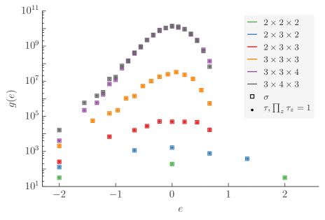
We collect numerical evidence in Fig. 2, that the variable transformation is genuinely following the same pattern as in the $1d$ and $2d$ cases discussed earlier. For very small lattices we exactly enumerated the models in Eqs. (22) and (29), (30) with the different spin representations for periodic boundaries. For some of the tested $3d$ lattice geometries with dimensions $\left(L_{x},L_{y},L_{z}\right)$ with $L_{i}\leq 4$ we compare in Fig. 2 the number of states $g_{\sigma}(E)$ with an energy $E=H(\{\sigma_{i}\})$. States that do not satisfy the $L_{x}\times L_{y}$ constraints in Eq. (30) are discarded during the enumeration to yield the number of states $g_{\tau}(E)$ for the $\tau$-representation. Finally, we respect the factors of $2$ from the transformation for the comparison, $g_{\sigma}(E)=2^{L_{x}L_{y}}g_{\tau}(E)$. For such small lattices, boundary effects yield the most prominent contributions. We also checked that our program yielded the same results when $L_{x}$ and $L_{y}$ were exchanged (not shown). We find that the (integer) numbers perfectly agree in all cases.

Figure 2: Number of states $g(e)$ over normalized energy $e=E/(L_{x}\times L_{y}\times L_{z})$ for the two representations of the fuki-nuke Hamiltonian with different lattice geometries under periodic boundary conditions. Boxes mark the number of states with a given energy $e$ for the $\sigma$-representation, dots mark the (rescaled) number of states $2^{L_{x}L_{y}}g_{\tau}(e)$ of states with energy $e$ in the $\tau$-representation. Since all dots fall into a box, the numbers agree.

To interpret the role of the constraints we employ formally the same trick from the $1d$ Ising model of rewriting the constraints in the partition function,

$$Z_{\rm fuki\mathchar 45\relax nuke} = 2^{L^{2}}\sum_{\{\tau\}}\exp\left(-\beta H_{\rm fuki\mathchar 45\relax nuke}(\{\tau\})\right)\prod_{x=1}^{L}\prod_{y=1}^{L}\delta\left(\prod_{z=1}^{L_{z}}\tau_{x,y,z},1\right)$$ (31)

$$= \sum_{\{\tau\}}\exp\left(-\beta H_{\rm fuki\mathchar 45\relax nuke}(\{\tau\})\right)\prod_{x=1}^{L}\prod_{y=1}^{L}\left(1+\prod_{z=1}^{L_{z}}\tau_{x,y,z}\right).$$

If we expand the $\prod_{x=1}^{L}\prod_{y=1}^{L}\left(1+\prod_{z=1}^{L_{z}}\tau_{x,y,z}\right)$ term in Eq. (31) with the common definition of the expectation value $\langle O\rangle_{Z}=Z^{-1}\sum_{\{\tau\}}Oe^{-\beta H}$ of an observable $O$ with respect to the Hamiltonian $H$ and partition function $Z=\sum_{\{\tau\}}e^{-\beta H}$, we find

$$Z_{\rm fuki\mathchar 45\relax nuke} = \sum_{\{\tau\}}\exp\left(-\beta H_{\rm fuki\mathchar 45\relax nuke}(\{\tau\})\right)\left(1+\sum_{x=1}^{L}\sum_{y=1}^{L}\prod_{z=1}^{L_{z}}\tau_{x,y,z}+\mathcal{O}\left(\tau\tau\right)\right)$$ (32)

$$= Z_{\rm fuki\mathchar 45\relax nuke}^{*}\left(1+\sum_{x=1}^{L}\sum_{y=1}^{L}\langle\prod_{z=1}^{L_{z}}\tau_{x,y,z}\rangle_{Z_{\rm fuki\mathchar 45\relax nuke}^{*}}+\mathcal{O}(\tau\tau)\right),$$

where $Z_{\rm fuki\mathchar 45\relax nuke}^{*}=Z_{\rm fuki\mathchar 45\relax nuke,\;free}/2^{L^{2}}=\left(Z_{2d\;\rm Ising}\right)^{L_{z}}$, similar to the calculation in Eq. 26, but without the outer sum from the extra plane (and $L_{z}\rightarrow L_{z}+1$). Noticing that the product of $\tau$’s factorizes over the layers, leads to the simplification

$$Z_{\rm fuki\mathchar 45\relax nuke} = \left(Z_{2d\;\rm Ising}\right)^{L_{z}}\left(1+\sum_{x=1}^{L}\sum_{y=1}^{L}\left(\langle\tau_{x,y}\rangle_{Z_{2d\;\rm Ising}}\right)^{L_{z}}+\mathcal{O}(\tau\tau)\right).$$ (33)

Finally, assuming translational invariance (i.e., periodic boundaries in each $2d$ Ising layer) the leading correction further simplifies to

$$Z_{\rm fuki\mathchar 45\relax nuke} = \left(Z_{2d,\;{\rm Ising}}\right)^{L_{z}}\left(1+L^{2}C_{1}^{L_{z}}+\mathcal{O}\left(\tau\tau\right)\right),$$ (34)

with $C_{1}=\langle\tau_{1,1}\rangle_{Z_{2d,\;{\rm Ising}}}$ being the normalized one-point function, or magnetization of the $2d$ Ising model, with its distinct features: it vanishes for finite lattices (layers), but due to spontaneous symmetry breaking assumes a non-zero value in the low-temperature phase when taking the thermodynamic limit in finite field prior to setting the field to zero. Here, in the fuki-nuke case, “field” corresponds in the original formulation with spins $\sigma_{x,y,z}$ to the coupling constant of a nearest-neighbour interaction in $z$-direction.

Similarly the $\mathcal{O}\left(\tau\tau\right)$ contribution in Eqs. (32)-(34) can be written as

$$\!\!\!\!\!\!\mathcal{O}\left(\tau\tau\right) = \frac{1}{2}\left(\sum_{x_{1}=1}^{L}\sum_{y_{1}=1}^{L}\sum_{x_{2}=1}^{L}\sum_{y_{2}=1}^{L}\langle\prod_{z=1}^{L_{z}}\tau_{x_{1},y_{1},z}\tau_{x_{2},y_{2},z}\rangle_{Z_{\rm fuki\mathchar 45\relax nuke}^{*}}-1\right)+\mathcal{O}\left(\tau\tau\tau\right)$$ (35)

$$= \frac{1}{2}\left(\sum_{x_{1}=1}^{L}\sum_{y_{1}=1}^{L}\sum_{x_{2}=1}^{L}\sum_{y_{2}=1}^{L}\left(\langle\tau_{x_{1},y_{1}}\tau_{x_{2},y_{2}}\rangle_{Z_{2d\;\rm Ising}}\right)^{L_{z}}-1\right)+\mathcal{O}\left(\tau\tau\tau\right)$$

which is a sum over all two-point functions of the $2d$ Ising model and hence a much more difficult expression to evaluate exactly [16]. Only the next-neighbour correlation, being proportional to the internal energy, is readily accessible for finite layers (with periodic boundary conditions) from the Kaufman solution [17]. Even if the power $L_{z}$ on each of the two-point functions in Eq. (35) would not be present, we would end up with the expression for the (high-temperature) susceptibility of the $2d$ Ising model. A closed-form expression for this is as yet unknown, although its properties have been analysed carefully to high precision using series expansions of extremely high order [18]. The next terms in Eq. (35) are of the form

$$\!\!\!\!\!\!\!\!\left(\langle\tau_{x_{1},y_{1}}\tau_{x_{2},y_{2}}\tau_{x_{3},y_{3}}\rangle_{Z_{2d\;\rm Ising}}\right)^{L_{z}},\quad\left(\langle\tau_{x_{1},y_{1}}\tau_{x_{2},y_{2}}\tau_{x_{3},y_{3}}\tau_{x_{4},y_{4}}\rangle_{Z_{2d\;\rm Ising}}\right)^{L_{z}},\quad\dots$$ (36)

for all possible combinations of $x_{1},y_{1},\dots,x_{4},y_{4},\dots$.

In summary, we have found that the products of vertical stacks of $\tau_{x,y,z}$ spins in $\prod_{z=1}^{L_{z}}\tau_{x,y,z}$ arising from the constraints due to periodic boundary conditions give contributions from (all) $n$-point Ising spin correlation functions (with $n\leq L^{2}$) in each layer to $Z_{\rm fuki\mathchar 45\relax nuke}$. While providing an explicit exact answer to the problem, this prevents the straightforward calculation of a closed-form expression for the fuki-nuke model with periodic boundaries in the manner of Eqs. (20) and (21) for the case of the $2d$ plaquette model with periodic boundaries.

A similar representation for $Z_{\rm fuki\mathchar 45\relax nuke}$ for periodic boundary conditions has been obtained previously by Jonsson and Savvidy [19] in a purely geometrical interpretation of the fuki-nuke model as a model for fluctuating random (closed) surfaces [8, 9]. By developing a suitable loop Fourier transformation they found the solution to the fuki-nuke partition function from eigenvalues of the transfer matrix between loops in the different layers (tracing the intersections with the closed surfaces). These eigenvalues can be expressed in terms of the partition function and correlation functions of the $2d$ Ising model, which can be identified with the corrections appearing in Eq. (34). The exact finite-size solution with periodic boundary conditions thus amounts to evaluating all $n$-point spin correlation functions in the $2d$ Ising model. This is a much more difficult task [16] than for the almost trivial case of free boundary conditions in Eq. (26), where no such correlation functions appear. It would be interesting to see how, in the latter case, such a simplification might occur in the geometrical surface/loop picture, too.

Figure 3: A dimer configuration of the fuki-nuke model with $L_{z}=3$ that can contribute to the partition function, although the mid and top layer have dangling ends (symbolised by open circles). These are connected through the constraints (dashed vertical lines) and contribute to the two-point function in each of the two upper layers. Notice that additional, standard $2d$ Ising loops may appear, as those shown in the bottom layer, which are the standard contributions to the partition function of each layer.

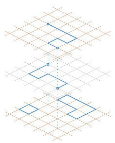
The high-temperature expansion/dimer picture employed in Sec. 3.2 allowed an explicit solution of the $2d$ plaquette model with periodic boundaries, where the constraints connect the different rows of spins with dangling ends (recall Fig. 1). We could employ a particle-gap symmetry there, easing the counting and effectively reducing the problem to a one-dimensional problem. A similar approach eludes us in $3d$ for the fuki-nuke model, however, where the equivalent picture leads to configurations with the constraints connecting the different layers, see Fig. 3. The dimer configurations with two dangling ends in the mid and top layer contribute to the two-point function. Counting closed loops for the $2d$ Ising model is already a non-trivial combinatorial problem, and here we have to deal with additional complexity depending on the number and position of the dangling ends. It is obvious that the difficulty of the problem grows rapidly with the number $n$ of dangling ends, contributing to the $n$-point function. While Eqs. (33)-(36) give the most explicit exact result, the high-temperature expansion/dimer approach is the most intuitive pictorial way to explain how the constraints for periodic boundary conditions induce the contributions of $n$-point correlations to the partition function of each layer, as illustrated in Fig. 3.

That one set of boundary conditions should admit a closed-form finite-size solution and another not, is of course seen in other models, too. A canonical example is the standard $2d$ Ising model where the exact solution on finite lattices is known only for cases where there are (anti)periodic or twisted boundary conditions in at least one direction [17, 20]. For very recent results on bulk, surface and corner free energies of the square lattice Ising model for the case of free boundaries, see [21].

5 Conclusions

Motivated originally by considerations from Monte Carlo simulations, where periodic boundary conditions are often employed in finite-size scaling studies and where the density of states is of interest for multicanonical methods, we investigated the differences between free and periodic boundary conditions in calculating the partition function of various Ising models using product spin transformations.

In $1d$ we observed that the partition function of the standard nearest-neighbour Ising model with periodic boundary conditions could be evaluated using product spins if the constraint arising from the boundary conditions was imposed via a convenient representation of the delta function.

Similar considerations were found to apply to a $2d$ plaquette Ising model, where the spin-bond transformations allowed exact evaluations of the partition function for free and periodic boundary conditions. Although equivalent to a $1d$ Ising model in the thermodynamic limit, the (boundary condition dependent) finite-size corrections for the $2d$ plaquette model are not identical.

In $3d$ we compared the formulation of an anisotropic $3d$ plaquette model, the fuki-nuke model, using product spin variables with free boundary conditions [1] to the case of periodic boundary conditions  [2]. In understanding the detailed differences between these the treatment of free and periodic boundary conditions in the $1d$ Ising model and $2d$ plaquette model provided a useful guide. For the fuki-nuke model the exact finite-size partition function may be written as a product of $2d$ Ising partition functions in the case of free boundary conditions using the product variable transformation. A similar decoupling is not manifest with periodic boundary conditions, where all $n$-point $2d$ Ising spin-spin correlations also contribute to the expression for the $3d$ fuki-nuke partition function. As illustrated in Fig. 3, this can be most easily understood in a pictorial way by employing the high-temperature expansion/dimer approach, whereas the exact result in Eqs. (33)-(36) displays the contributing terms in the most explicit manner. It is perhaps worth remarking that the discussion of the fuki-nuke model in [2] conflates the discussion of free and periodic boundary conditions, although the overall picture of a $2d$ Ising-like transition in the thermodynamic limit of the $3d$ fuki-nuke model remains, of course, correct in both cases.

The key point to be drawn from the various exact solutions explored in this paper is that finite-size corrections due to periodic boundary conditions may be viewed as coming from induced correlations, which may be a useful point of view when carrying out finite-size scaling analyses of numerical results.

References

Appendix A Two Dimensions: Helical Boundary Conditions by High-T Representation and Combinatorics

Helical boundary conditions have already been used when comparing the $2d$ gonihedric Ising model with a $1d$ Ising model by means of Metropolis Monte Carlo simulations [15], although here the finite-size scaling was not investigated since the focus was on the dynamical properties of the model.

We assume helical boundary conditions in $x$-direction, i.e., $\sigma_{L_{x}+1,y}=\sigma_{1,y+1}$, and periodic boundaries in $y$-direction. The latter choice is not arbitrary, because the next-to-nearest-neighbour interactions in the Hamiltonian forbid helical boundaries in $y$-direction, or else one may find different spins on the boundaries depending on whether one first goes along the $x$-axis or $y$-axis.

The partition function for helical boundaries can be found by counting the possible contributions when expanding the product in the high-temperature representation in Eq. (19). As in the periodic case, only those configurations can contribute to the partition function whose spins appear with an even power. An arbitrarily chosen plaquette on an empty lattice has one spin on each of the four corners and each spin contributes only once. For this plaquette to contribute, adjacent plaquettes must also contribute, either connected through a common bond or through a corner. Valid configurations are thus either combinations of columns in $y$-direction that are closed through the periodic boundary conditions, one complete row that is closed with help of the helical boundaries or checker board configurations. Checker board configurations only appear for lattices with an even number $L_{y}$ of spins in the direction of the periodic boundaries, and here each column can have two possible patterns as depicted in Fig. 1. Hence, for odd $L_{y}$ we find

$$Z_{2d,\;{\rm gonihedric},\;{\rm helical},\;{\rm periodic}}=2^{L_{x}L_{y}}\operatorname{ch}(\beta)^{L_{x}L_{y}}\left(1+\operatorname{th}(\beta)^{L_{y}}\right)^{L_{x}},$$ (37)

and for lattices with even $L_{y}$,

$$\qquad Z_{2d,\;{\rm gonihedric},\;{\rm helical},\;{\rm periodic}} =$$ (38)

$$2^{L_{x}L_{y}}\operatorname{ch}(\beta)^{L_{x}L_{y}} \left(\left(1+\operatorname{th}(\beta)^{L_{y}}\right)^{L_{x}}+2^{L_{x}}\operatorname{th}(\beta)^{L_{x}L_{y}/2}\right),$$

where the additional term accounts for the contributions from checker-board-like configurations, where the $L_{x}\times L_{y}/2$ plaquettes contribute a $\operatorname{th}(\beta)$ each. The freedom of column-wise switching of gray and white plaquettes is reflected in the prefactor $2^{L_{x}}$.

(a) b

(b) b

(c) b

Figure 1: Illustration of checker board configurations with helical boundaries along the $x$-direction and periodic boundaries in $y$-direction. The thick green lines separate repeating units of the system. Numbers distinguish the different plaquettes that are “active” (gray) or “inactive” (white). (a) For lattices with an odd number $L_{y}$ of plaquettes in $y$-direction, edges are created with spins that contribute to $3$ plaquettes (here, the black dot). Hence, that configuration does not appear in the partition function. (b) For even $L_{y}$, the checker board can be continued over the boundaries without having spins contribute with odd power. (c) In each column the gray and white plaquettes can be switched, leading to another valid configuration. Here, the second column of (b) has been switched.

References

- [1] M. Suzuki, Phys. Rev. Lett. 28 (1972) 507.
- [2] C. Castelnovo, C. Chamon and D. Sherrington, Phys. Rev. B 81 (2010) 184303.
-
[3]
Y. Hashizume and M. Suzuki, Int. J. Mod. Phys. B 25 (2011) 73;
Y. Hashizume and M. Suzuki, Int. J. Mod. Phys. B 25 (2011) 3529. -
[4]
D. A. Johnston,
J. Phys. A: Math. Theor. 45 (2012) 405001;
M. Mueller, D. A. Johnston and W. Janke, Nucl. Phys. B 894 (2015) 1;
D. A. Johnston, M. Mueller and W. Janke, Mod. Phys. Lett. B 29 (2015) 1550109. - [5] D. Espriu, M. Baig, D. A. Johnston and R. P. K. C. Malmini, J. Phys. A: Math. Gen. 30 (1997) 405.
[6]
M. Mueller, W. Janke and D. A. Johnston,
Phys. Rev. Lett. 112 (2014) 200601;
M. Mueller, D. A. Johnston and W. Janke, Nucl. Phys. B 888 (2014) 214. -
[7]
A. Lipowski, J. Phys. A: Math. Gen. 30 (1997) 7365;
A. Lipowski and D. A. Johnston, J. Phys. A: Math. Gen. 33 (2000) 4451;
A. Lipowski and D. A. Johnston, Phys. Rev. E 61 (2000) 6375;
M. Swift, H. Bokil, R. Travasso and A. Bray, Phys. Rev. B 62 (2000) 11494;
D. A. Johnston, A. Lipowski and R. P. K. C. Malmini, in Rugged Free Energy Landscapes: Common Computational Approaches to Spin Glasses, Structural Glasses and Biological Macromolecules, ed. W. Janke, Lecture Notes in Physics 736 (Springer, Berlin, 2008), p. 173. - [8] R. V. Ambartzumian, G. K. Savvidy, K. G. Savvidy and G. S. Sukiasian, Phys. Lett. B 275 (1992) 99; G. K. Savvidy and K. G. Savvidy, Mod. Phys. Lett. A 08 (1993) 2963; G. K. Savvidy and K. G. Savvidy, Int. J. Mod. Phys. A 08 (1993) 3993.
- [9] G. K. Savvidy and F. J. Wegner, Nucl. Phys. B 413 (1994) 605; G. K. Savvidy and K. G. Savvidy, Phys. Lett. B 324 (1994) 72; G. K. Bathas, E. Floratos, G. K. Savvidy and K. G. Savvidy, Mod. Phys. Lett. A 10 (1995) 2695; G. K. Savvidy, K. G. Savvidy and P. G. Savvidy, Phys. Lett. A 221 (1996) 233.
[10]
Loïc Turban, in Phénomènes Critiques-V, Modèles Exactement Solubles,
at http://gps.ijl.univ-lorraine.fr/webpro/turban.l - [11] E. Ising, Z. Phys. 31 (1925) 253.
- [12] R. L. Jack, L. Berthier and J. P. Garrahan, Phys. Rev. E 72 (2005) 016103.
- [13] M. Kac and J. C. Ward, Phys. Rev. 88 (1952) 1332; R. P. Feynman, Statistical Mechanics. A Set of Lectures (The Benjamin and Cummings Publishing Co., Reading, Massachusetts, 1972).
- [14] D. Espriu and A. Prats, Phys. Rev. E 70 (2004) 046117.
- [15] S. Davatolhagh, D. Dariush and L. Separdar, Phys. Rev. E 81 (2010) 031501.
[16]
B. M. McCoy and T. T. Wu, The Two-Dimensional Ising Model (Harvard University Press, Cambridge, 1973);
R. J. Baxter, Exactly Solved Models in Statistical Mechanics (Academic Press, New York, 1982). -
[17]
B. Kaufman,
Phys. Rev. 76 (1949) 1232;
A. E. Ferdinand and M. E. Fisher, Phys. Rev. 185 (1969) 832. -
[18]
B. Nickel, J. Phys. A: Math. Gen. 32 (1999) 3889;
B. Nickel, J. Phys. A: Math. Gen. 33 (2000) 1693;
W. P. Orrick, B. G. Nickel, A. J. Guttmann and J. H. H. Perk, Phys. Rev. Lett. 86 (2001) 4120;
W. P. Orrick, B. G. Nickel, A. J. Guttmann and J. H. H. Perk, J. Stat. Phys. 102 (2001) 795;
S. Boukraa, A. J. Guttmann, S. Hassani, I. Jensen, J.-M. Maillard, B. Nickel and N. Zenine, J. Phys. A: Math. Theor. 41 (2008) 455202;
Y. Chan, A. J. Guttmann, B. G. Nickel and J. H. H. Perk, J. Stat. Phys. 145 (2011) 549. -
[19]
T. Jonsson and G. K. Savvidy, Phys. Lett. B 449 (1999) 253;
T. Jonsson and G. K. Savvidy, Nucl. Phys. B 575 (2000) 661;
G. K. Savvidy, J. High Energy Phys. 09 (2000) 44;
G. K. Savvidy, Mod. Phys. Lett. B 29 (2015) 1550203. -
[20]
L. Onsager, Phys. Rev. 65 (1944) 117;
H. J. Brascamp and H. Kunz, J. Math. Phys. 15 (1974) 66;
D. L. O’Brien, P. A. Pearce and S. O. Warnaar, Physica A 228 (1996) 63;
W. T. Lu and F. Y. Wu, Physica A 258 (1998) 157;
W. T. Lu and F. Y. Wu, Phys. Rev. E 63 (2001) 026107;
M. C. Wu and C. K. Hu, J. Phys. A: Math. Gen. 35 (2002) 5189;
T. M. Liaw, M. C. Huang, Y. L. Chou, S. C. Lin and F. Y. Li, Phys. Rev. E 73 (2006) 055101(R);
A. Poghosyan, R. Kenna and N. Izmailian, Europhys. Lett. 111 (2015) 60010. -
[21]
R. J. Baxter, arXiv:1606.02029v3 [math-ph];
E. Vernier and J. L. Jacobsen, J. Phys. A: Math. Theor. 45 (2012) 045003.