The John–Nirenberg constant of ${\rm BMO}^{p},$ $p>2$

Abstract.

This paper is a continuation of earlier work by the first author who determined the John–Nirenberg constant of ${\rm BMO}^{p}\big{(}(0,1)\big{)}$ for the range $1\leq p\leq 2.$ Here, we compute that constant for $p>2.$ As before, the main results rely on Bellman functions for the ${\color[rgb]{0,0,0}L^{p}}$ norms of logarithms of $A_{\infty}$ weights, but for $p>2$ these functions turn out to have a significantly more complicated structure than for $1\leq p\leq 2.$

1. Preliminaries and main results

For a finite interval $J$ and a function $\varphi\in L^{1}(J),$ let $\langle\varphi\rangle_{{}_{\scriptstyle J}}$ denote the average of $\varphi$ over $J$ with respect to the Lebesgue measure, $\langle\varphi\rangle_{{}_{\scriptstyle J}}=\frac{1}{|J|}\int_{J}\varphi.$ Take an interval $Q$ and $p>0,$ and let ${\rm BMO}(Q)$ be the (factor-)space

(1.1) $${\rm BMO}(Q)=\{\varphi\in L^{1}{\color[rgb]{0,0,0}(Q)}\colon\quad\|\varphi\|_{{\rm BMO}^{p}(Q)}:=\sup_{\text{interval}~{}J\subset Q}\langle|\varphi-\langle\varphi\rangle_{{}_{\scriptstyle J}}|^{p}\rangle_{{}_{\scriptstyle J}}^{1/p}<\infty\}.$$

It is a classical fact that all $p$-based (quasi-)norms are equivalent, which justifies omitting the index $p$ in the left-hand side.

A weight is an almost everywhere positive function. We say that a weight $w$ belongs to $A_{\infty}(Q),$ $w\in A_{\infty}(Q),$ if both $w$ and $\log w$ are integrable on $Q$ and the following condition holds:

$$[w]_{A_{\infty}(Q)}:=\sup_{\text{interval~{}}J\subset Q}\langle w\rangle_{{}_{\scriptstyle J}}e^{-\langle\log w\rangle_{{}_{\scriptstyle J}}}<\infty.$$

The quantity $[w]_{A_{\infty}(Q)}$ is called the $A_{\infty}(Q)$-characteristic of $w.$ When $Q$ is fixed or unimportant, we write simply ${\rm BMO}$ for ${\rm BMO}(Q)$ and $A_{\infty}$ for $A_{\infty}(Q).$

BMO functions are locally exponential integrable. We can state this property in the form of the so-called integral John–Nirenberg inequality, which is a variant of the classical weak-type inequality from [5].

Theorem (John–Nirenberg).

Take $p>0.$ There exists a number $\varepsilon_{0}(p)>0$ such that if $\varepsilon\in[0,\varepsilon_{0}(p)),$ $Q$ is an interval, and $\varphi\in{\rm BMO}(Q)$ with $\|\varphi\|_{\scriptscriptstyle{\rm BMO}^{p}(Q)}\leq\varepsilon,$ then there is a number $C(\varepsilon,p)>0$ such that for any interval $J\subset Q,$

(1.2) $$\langle e^{\varphi}\rangle_{{}_{\scriptstyle J}}\leq C(\varepsilon,p)e^{\langle\varphi\rangle_{{}_{\scriptstyle\scriptscriptstyle J}}}.$$

We will always use $\varepsilon_{0}(p)$ to denote the best – largest possible – constant in this theorem and call it the John–Nirenberg constant of ${\rm BMO}^{p}$ (on an interval). Likewise, $C(\varepsilon,p)$ will denote the smallest possible constant in (1.2).

Observe that (1.2) means that if $\varphi\in{\rm BMO},$ then $e^{\varepsilon\varphi}\in A_{\infty}$ for all sufficiently small $\varepsilon>0.$ For $\varphi\in{\rm BMO},$ let

(1.3) $${\color[rgb]{0,0,0}\varepsilon_{\varphi}=\sup\{\varepsilon:~{}e^{\varepsilon\varphi}\in A_{\infty}\}.}$$

In fact, it can be shown that

$${\color[rgb]{0,0,0}\varepsilon_{0}(p)=\inf\{\varepsilon_{\varphi}:~{}\|\varphi\|_{{\rm BMO}^{p}}\!=\!1\}=\sup\{\varepsilon:~{}\forall\varphi,~{}\|\varphi\|_{{\rm BMO}^{p}}\!=\!1~{}\Longrightarrow~{}e^{\varepsilon\varphi}\in A_{\infty}\}}.$$

In this paper, our goal is to compute $\varepsilon_{0}(p)$ for the case $p>2.$ Here are some previous results in that direction: Korenovskii [6] and Lerner [7] computed the analogs for the weak-type John–Nirenberg inequality of $\varepsilon_{0}(1)$ and $C(\varepsilon,1),$ respectively; in [9], we determined $\varepsilon_{0}(2)$ and $C(\varepsilon,2);$ in [12], the second author and A. Volberg found all constants in the weak-type inequality for $p=2;$ and, finally, in [8], the first author determined $\varepsilon_{0}(p)$ for $p\in[1,2]$ and $C(\varepsilon,p)$ for $p\in(1,2]$ and large enough $\varepsilon.$ This last paper built the framework that we follow here, and we refer the reader to it for an in-depth discussion of the tools involved and the differences between the cases $p=2$ and $p\neq 2.$

Let us state the relevant theorem from [8].

Theorem 1.1 ([8]).

For $p\in[1,2]$,

$$\varepsilon_{0}(p)=\left[\frac{p}{e}\Big{(}\Gamma(p)-\int_{0}^{1}t^{p-1}e^{t}\,dt\Big{)}+1\right]^{1/p}.$$

Furthermore, if $1<p\leq 2,$ then for all $(2-p)\varepsilon_{0}(p)\leq\varepsilon<\varepsilon_{0}(p),$

(1.4) $$C(\varepsilon,p)=\frac{e^{-\varepsilon/\varepsilon_{0}(p)}}{1-\varepsilon/\varepsilon_{0}(p)};$$

and for all $0\leq\varepsilon<\frac{2}{e},$

(1.5) $$\frac{e^{-\frac{e}{2}\varepsilon}}{1-\frac{e}{2}\varepsilon}\leq C(\varepsilon,1)\leq\frac{1}{1-\frac{e}{2}\,\varepsilon}.$$

We can finally complete the picture for all $p\geq 1.$ Remarkably, the formula for $\varepsilon_{0}(p)$ for the case $p>2$ is the same as for $1\leq p\leq 2,$ though it takes much more work to show.

Theorem 1.2.

For $p>2$,

(1.6) $$\varepsilon_{0}(p)=\left[\frac{p}{e}\Big{(}\Gamma(p)-\int_{0}^{1}t^{p-1}e^{t}\,dt\Big{)}+1\right]^{1/p}.$$

In contrast with the case $1<p\leq 2,$ for $p>2$ we do not know the exact $C(\varepsilon,p)$ for any $\varepsilon.$ While we could estimate this constant in a manner somewhat similar to (1.5), the estimates we currently have seem much too implicit to be useful, so we omit them.

Without going into details, we mention another, more important difference between the cases $p\leq 2$ and $p>2.$ It was shown in [8] that the constant $\varepsilon_{0}(p)$ is attained in the weak-type John–Nirenberg inequality for $1<p\leq 2$ (the case $p=1$ was treated in [6] and [7], while the case $p=2$ had been previously addressed in [12]). However, the method used to show this fact for $p\leq 2$ fails for $p>2,$ and we do not actually know if the constant is attained (though we conjecture that it is).

On the other hand, still another interesting result from [8] does go through for $p>2.$ Specifically, we have the following theorem, which extends to $p>2$ the main result of Corollary 1.5 from [8]. It is a sharp lower estimate for the distance in ${\rm BMO}$ to $L^{\infty}$ in the spirit of Garnett and Jones [1].

Theorem 1.3.

If $p>2,$ $Q$ is an interval, and $\varphi\in{\rm BMO}(Q),$ then

(1.7) $$\inf_{f\in L^{\infty}(Q)}\|\varphi-f\|_{{\rm BMO}^{p}(Q)}\geq\frac{\varepsilon_{0}(p)}{\min\{\varepsilon_{\varphi},\varepsilon_{-\varphi}\}},$$

and this inequality is sharp.

As explained in [8], the main idea for computing $\varepsilon_{0}(p)$ for $p\neq 2$ is to consider the dual problem: instead of estimating for which values of $\|\varphi\|_{{\rm BMO}^{p}}$ the exponential oscillation $\langle e^{\varphi-\langle\varphi\rangle}\rangle$ might become unbounded, one estimates from below ${\rm BMO}^{p}$ oscillations of logarithms of $A_{\infty}$ weights and computes their asymptotics as the $A_{\infty}$-characteristic goes to infinity. This idea is formalized in the following general theorem.

Fix $p>0.$ For $C\geq 1,$ let

(1.8) $$\Omega_{C}=\{x\in\mathbb{R}^{2}:e^{x_{1}}\leq x_{2}\leq C\,e^{x_{1}}\}.$$

For an interval $Q{\color[rgb]{0,0,0},}$ $C\geq 1,$ and every $x=(x_{1},x_{2})\in\Omega_{C},$ let

(1.9) $$E_{x,C,Q}=\{\varphi\in L^{1}(Q):~{}\langle\varphi\rangle_{{}_{\scriptstyle Q}}=x_{1},~{}\langle e^{\varphi}\rangle_{{}_{\scriptstyle Q}}=x_{2},~{}[e^{\varphi}]_{A_{\infty}(Q)}\leq C\}.$$

We will call elements of $E_{x,C,Q}$ test functions. Define the following lower Bellman function:

(1.10) $$\boldsymbol{b}_{p,C}(x)=\inf\{\langle|\varphi|^{p}\rangle_{{}_{\scriptstyle Q}}:~{}\varphi\in E_{x,C,Q}\}.$$

Theorem 1.4 ([8]).

Take $p>0.$ Assume that there exists a family of functions $\{b_{C}\}_{C\geq 1}$ such that for each $C{\color[rgb]{0,0,0},}$ $b_{C}$ is defined on $\Omega_{C},$ $b_{C}\leq\boldsymbol{b}_{p,C},$ and $b_{C}(0,\cdot)$ is continuous on the interval $[1,C].$ Then

(1.11) $$\varepsilon^{p}_{0}(p)\geq\limsup_{C\to\infty}b_{C}(0,C).$$

Thus, to estimate $\varepsilon_{0}(p),$ we need a suitable family $\{b_{C}\}_{C}$ of minorants of $\boldsymbol{b}_{p,C}.$ Just as was done in [8], we actually find the functions $\boldsymbol{b}_{p,C}$ themselves, for all $p>2$ and all sufficiently large $C.$ We proceed as follows: in Section 2, for each suitable choice of $p$ and $C$ we construct the so-called Bellman candidate, denoted $b_{p,C}.$ This construction is more delicate and more technical than the one in [8], and we briefly discuss the challenges involved. The proof that $b_{p,C}\leq\boldsymbol{b}_{p,C}$ constitutes Section 3. In Section 5, we obtain the converse inequality by demonstrating explicit test functions that realize the infimum in (1.10). It is then an easy matter to prove Theorems 1.2 and 1.3, and it is taken up in Section 4.

2. The construction of the Bellman candidate

For $R>0,$ let

$$\Gamma_{R}=\{x\in\mathbb{R}^{2}:~{}x_{2}=Re^{x_{1}}\}.$$

Then the domain $\Omega_{C}$ from (1.8) is the region in the plane lying between $\Gamma_{1}$ and $\Gamma_{C}.$

2.1. Discussion and preliminaries

As mentioned earlier, the construction of the Bellman candidate given here for the case $p>2$ is different from and quite more involved than those presented in [8] for the cases $p=1$ and $p\in(1,2].$ However, the main goal is the same as before and simple to state: we are building the largest locally convex function $b$ on $\Omega_{C}$ satisfying the boundary condition $b(x_{1},e^{x_{1}})=|x_{1}|^{p}.$

Let us briefly explain the similarities and differences between the cases $p\in(1,2]$ and $p>2$ (the case $p=1$ is different from both). In both cases the graph of the candidate $b$ is a convex ruled surface, which means that through each point on the graph there passes a straight-line segment contained in the graph. The domain $\Omega_{C}$ then splits into a collection of subdomains with disjoint interiors, $\Omega_{C}=\cup_{j}R_{j},$ such that $b$ is twice differentiable and satisfies the homogeneous Monge–Ampère equation $b_{x_{1}x_{1}}b_{x_{2}x_{2}}=b^{2}_{x_{1}x_{2}}$ in the interior of each $R_{j}.$ In addition, each $R_{j}$ is foliated by straight-line segments connecting two points of the boundary $\Gamma_{1}\cup\Gamma_{C},$ and each point $x\in{\rm int}(R_{j})$ lies on only one such segment, unless $b$ is affine in the whole $R_{j}.$ We call such segments Monge–Ampère characteristics of $b.$ Typically, if one knows the characteristics everywhere in $\Omega_{C},$ one knows the function $b.$

Thus, to construct the candidate one has to understand how to split $\Omega_{C}$ into subdomains and how to foliate each of them, so that the resulting function $b$ is locally convex. If this is done while ensuring certain compatibility conditions, then $b$ will almost automatically be the largest locally convex function with the given boundary conditions, as desired. This is, in general, a difficult task, and the situation is further complicated by the fact that the splitting is usually different for different $C.$

Fortunately, there is now a fairly general theory for building such foliations on special non-convex domains such as ours. It was started in [10] in the context of ${\rm BMO}^{2};$ much developed and systematized in the papers [2] and [3], still for the parabolic strip of ${\rm BMO}^{2};$ and is now being adapted to general domains, such as $\Omega_{C},$ in [4]. We also mention the recent paper [11], which formalized the theoretical link between Bellman functions and smallest locally concave (or largest locally convex, as is the case here) functions on the corresponding domains.

A key building block for many Monge–Ampère foliations is the tangential foliation. Let us explain this notion in our setting.

For $C\geq 1,$ let $\xi=\xi(C)$ be the unique non-negative solution of the equation

$$e^{-\xi}=C(1-\xi):\quad 0\leq\xi<1.$$

Note that $\xi(1)=0$ and that $\xi$ is strictly increasing with $\lim_{C\to\infty}\xi(C)=1.$ Let

(2.1) $$k(z)=\frac{e^{z}}{1-\xi},\quad z\in\mathbb{R},$$

and define a new function $u=u(x)$ on $\Omega_{C}$ by the implicit formula

(2.2) $$x_{2}=k(u)(x_{1}-u)+e^{u}.$$

This function has simple geometrical meaning, illustrated in Figure 1: if one draws the one-sided tangent to $\Gamma_{C}$ that passes through $x,$ so that the point of tangency is to the right of $x,$ then this tangent intersects $\Gamma_{1}$ at the point $(u,e^{u}),$ while the point of tangency is $(u+\xi,Ce^{u+\xi}).$ In particular $u(0,C)=-\xi.$ (We note that in [8], $\xi$ and $u$ were called $\xi^{+}$ and $u^{+},$ respectively).

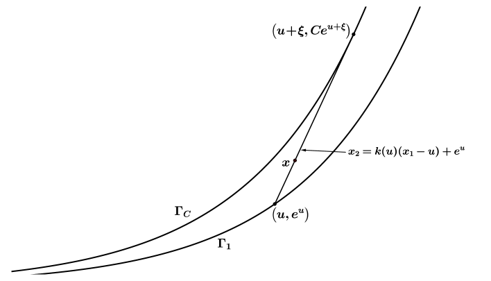
Figure 1. The geometric meaning of $u(x)$ and $\xi$

In the case $1<p\leq 2,$ if $C$ was large enough, all of $\Omega_{C}$ was foliated by the tangents (2.2), for $u\in(-\infty,\infty);$ thus, we did not have to split it into subdomains. However, for $p>2,$ this uniform tangential foliation fails to yield a locally convex function on the whole $\Omega_{C},$ for any $C.$ What actually happens — and, again, only for sufficiently large $C$ — is shown on Figure 2 later in this section. There we have two tangentially foliated subdomains, $R_{1}$ and $R_{3},$ which are linked by a special “transition regime” consisting of two more subdomains: $R_{4},$ where the candidate is affine and the foliation is thus degenerate, and $R_{2},$ where the characteristics are chords connecting two points of $\Gamma_{1}.$ (In recent Bellman-function literature, these two particular shapes are called “trolleybus” and “cup”, respectively; see [2, 3, 4].) This transition regime shrinks as $C$ grows, but never disappears. To show how all this fits together, we need some technical preparation.

2.2. Technical lemmas

Lemma 2.1.

1. If $w>0$ and $v\in\big{(}-w,-w\,\frac{p-1}{p}\big{)},$ then

   (2.3) $$\frac{w^{p-1}+(-v)^{p-1}}{e^{w}-e^{v}}<(p-1)(-v)^{p-2}e^{-v}.$$

2. If $0<w\leq\frac{p-2}{p-1}$ and $v\in(-w,0),$ then

   (2.4) $$\frac{w^{p-1}+(-v)^{p-1}}{e^{w}-e^{v}}<(p-1)w^{p-2}e^{-w}.$$

Proof.

For Part (1), note that $e^{w-v}-1\geq w-v>0,$ and so it is sufficient to check that

$$w^{p-1}+(-v)^{p-1}<(p-1)(-v)^{p-2}(w-v)\,.$$

Put $\theta={\color[rgb]{0,0,0}-\frac{v}{w}};$ then this inequality becomes

$$(p-2)\theta^{p-1}+(p-1)\theta^{p-2}-1>0\,,\qquad\frac{p-1}{p}<\theta<1\,.$$

The left-hand side is increasing in $\theta,$ and equals $2\frac{(p-1)^{{\color[rgb]{0,0,0}p}}}{p^{p-1}}-1$ when $\theta=\frac{p-1}{p}.$ In turn, this is an increasing function of $p,$ equal to 0 at $p=2$.

For Part (2), observe that since $w>-v,$ and $1-w\geq 1-\frac{p-2}{p-1}=\frac{1}{p-1},$ we have

$$1-e^{-(w-v)}>(w-v)\Big{[}1-\frac{1}{2}(w-v)\Big{]}>(w-v)(1-w)\geq\frac{w-v}{p-1},$$

and (2.4) follows from the obvious relation $w^{p-1}+(-v)^{p-1}<w^{p-2}(w-v).$ ∎

For any $v<0$ and $w>0,$ let

(2.5) $$r(u,w)=\frac{e^{w}-e^{v}}{w-v},\qquad q(v,w)=\frac{w^{p}-(-v)^{p}}{w-v}.$$

Lemma 2.2.

For each $w\in\big{(}0,\frac{p-2}{3p}\big{)},$ there exists a unique $v\in\big{(}-w,-w\,\frac{p-1}{p}\big{)}$ such that

(2.6) $$\frac{q(v,w)+p(-v)^{p-1}}{r(v,w)-e^{v}}=\frac{pw^{p-1}-q(v,w)}{e^{w}-r(v,w)}=p\,\frac{w^{p-1}+(-v)^{p-1}}{e^{w}-e^{v}}.$$

Proof.

Observe that it is enough to show only the first equality in (2.6), as the second one then follows by elementary rearrangement. In turn, this first equality is equivalent to the statement

(2.7) $$F(v,w):=(e^{w}-e^{v})(w^{p}-(-v)^{p}-pw^{p-1}-p(-v)^{p-1})+p(w-v)(w^{p-1}e^{v}+(-v)^{p-1}e^{w})=0.$$

Assume $w\in(0,\frac{p-2}{3p})$ and let $\lambda=\frac{p-1}{p}.$ To show that there exists $v\in(-w,-\lambda w)$ such that $F(v,w)=0,$ we compare the signs of $F(-w,w)$ and $F(-\lambda w,w).$

Since $F(-w,w)=4pw^{p-1}(w\cosh w-\sinh w)>0,$ we want to check that $F(-\lambda w,w)<0.$ To that end,

$$F(-\lambda w,w) =(e^{w}-e^{-\lambda w})\big{[}(1-\lambda^{p})w^{p}-p(1+\lambda^{p-1})w^{p-1}\big{]}+p(1+\lambda)w^{p}\big{[}e^{-\lambda w}+\lambda^{p-1}e^{w}\big{]},$$

and the inequality $F(-\lambda w,w)<0$ is equivalent to

$$\frac{(1+\lambda)w}{e^{(1+\lambda)w}-1}-1+\frac{1+p\lambda^{p-1}+(p-1)\lambda^{p}}{p(1+\lambda^{p-1})}w<0.$$

Let

$$\psi(t)=\frac{t}{e^{t}-1}-1+\frac{1+p\lambda^{p-1}+(p-1)\lambda^{p}}{p(1+\lambda)(1+\lambda^{p-1})}t\,.$$

We would like to show that $\psi(t)<0$ for $t\in(0,\frac{p-2}{3p}(1+\lambda))$. Note that for $t>0,$

$$e^{t}>1+t+\frac{1}{2}t^{2}\quad\implies\quad\frac{t}{e^{t}-1}-1<-\frac{t}{t+2}\,.$$

Therefore, for $t>0,$

$$\psi(t)<-t\Big{[}\frac{1}{t+2}-\frac{1+p\lambda^{p-1}+(p-1)\lambda^{p}}{p(1+\lambda)(1+\lambda^{p-1})}\Big{]},$$

and it is sufficient to check that

$$\frac{p-2}{3p}(1+\lambda)<\frac{p(1+\lambda)(1+\lambda^{p-1})}{1+p\lambda^{p-1}+(p-1)\lambda^{p}}-2=\frac{(p-2)(1-\lambda^{p})+p\lambda(1-\lambda^{p-2})}{1+p\lambda^{p-1}+(p-1)\lambda^{p}}.$$

Since $(p-2)(1-\lambda^{p})+p\lambda(1-\lambda^{p-2})>(p-2)(1+\lambda)(1-\lambda^{p-1})$ and $\lambda^{p}<\lambda^{p-1},$ it is enough to verify that

$$3>\frac{1/p+(2-1/p)\lambda^{p-1}}{1-\lambda^{p-1}}=\frac{2}{1-\lambda^{p-1}}-2+1/p.$$

This is so because the right-hand side is decreasing in $p$ and equals $\frac{5}{2}$ when $p=2.$ This proves that the desired $v$ exists for each $w.$

To show that $v$ is unique, we differentiate the function $F$ with respect to $v.$ This derivative can be written as follows:

$$F_{v}(v,w) =\big{(}e^{w}(w-v)-e^{w}+e^{v}\big{)}e^{v}\left(\frac{pw^{p-1}(w-v)-w^{p}+(-v)^{p}}{e^{w}(w-v)-e^{w}+e^{v}}-p(p-1)(-v)^{p-2}e^{-v}\right)$$

$$=\big{(}e^{w}(w-v)-e^{w}+e^{v}\big{)}e^{v}\left(p\,\frac{w^{p-1}+(-v)^{p-1}}{e^{w}-e^{v}}-p(p-1)(-v)^{p-2}e^{-v}\right),$$

where we used the second equality in (2.6). Now, the first factor is positive, because the function $t\mapsto e^{t}$ is strictly convex, while the last factor is negative by (2.3). Therefore, $F_{v}(v,w)$ is negative for any root $v$ of the equation $F(v,w)=0$ that lies in the interval $\big{(}-w,-w\,\frac{p-1}{p}\big{)},$ which is possible only when such a root is unique. ∎

From now on, in using $v$ and $w$ we will always presume that $w\in(0,\frac{p-2}{3p}),$ $v\in(-w,-w\,\frac{p-1}{p}),$ and the pair $\{v,w\}$ is related by equation (2.6). For such $v$ and $w,$ each of the three equal quantities in (2.6) is a function of $w,$ and it is convenient to give them a common name. Let

(2.8) $$D(w)=\frac{q(v,w)+p(-v)^{p-1}}{r(v,w)-e^{v}}=\frac{pw^{p-1}-q(v,w)}{e^{w}-r(v,w)}=p\,\frac{w^{p-1}+(-v)^{p-1}}{e^{w}-e^{v}},$$

and $D$ is a function of $w$ defined on the interval $\big{(}0,\frac{p-2}{3p}\big{)}.$ Let us list some of its properties.

Lemma 2.3.

We have

(2.9) $$D(w)<p(p-1)(-v)^{p-2}e^{-v}$$

and

(2.10) $$D(w)<p(p-1)w^{p-2}e^{-w}.$$

Furthermore, $D^{\prime}>0$ on $\big{(}0,\frac{p-2}{3p}\big{)}.$

Proof.

Inequalities (2.9) and (2.10) come directly from (2.3) and (2.4), respectively (note that $\frac{p-2}{3p}<\frac{p-2}{p-1},$ so (2.4) applies).

To check the sign of $D,$ we will treat $q$ and $r$ as functions of $w$ and use the prime to indicate the total derivative with respect to $w.$ Thus, $q^{\prime}=q_{w}+q_{v}v_{w}$ and $r^{\prime}=r_{w}+r_{v}v_{w},$ where $v_{w}$ can be computed from equation  (2.7). Also denote $f(w):=w^{p}$ and $g(w):=e^{w}.$

We will need the simple but key fact that equation (2.6) can be written as

(2.11) $$\frac{q^{\prime}}{r^{\prime}}=\frac{q-f^{\prime}}{r-g^{\prime}}=D.$$

Using this identity, we have

$$D^{\prime} =\Big{(}\frac{q-f^{\prime}}{r-g^{\prime}}\Big{)}^{\prime}=\frac{(q^{\prime}-f^{\prime\prime})(r-g^{\prime})-(q-f^{\prime})(r^{\prime}-g^{\prime\prime})}{(r-g^{\prime})^{2}}$$

$$=\frac{g^{\prime\prime}(q-f^{\prime})-f^{\prime\prime}(r-g^{\prime})}{(r-g^{\prime})^{2}}=\frac{g^{\prime\prime}}{r-g^{\prime}}\,\Big{(}\frac{q-f^{\prime}}{r-g^{\prime}}-\frac{f^{\prime\prime}}{g^{\prime\prime}}\Big{)}.$$

Since $g$ is strictly convex, we have $g^{\prime\prime}>0$ and $r-g^{\prime}<0.$ On the other hand, the expression in parentheses is negative by  (2.10). ∎

For $p>2,$ let

(2.12) $$\xi_{0}(p)=1-\frac{1}{3^{p+2}\Gamma(p)},\qquad C_{0}(p)=\frac{e^{-\xi_{0}(p)}}{1-\xi_{0}(p)}.$$

Lemma 2.4.

Assume $\xi>\xi_{0}(p).$ Let

$$c_{1}=\xi\big{[}e(1-\xi)\Gamma(p-1)\big{]}^{1/(p-2)},\qquad c_{2}=\xi\big{[}2e(1-\xi)\Gamma(p)\big{]}^{1/(p-2)}.$$

Then the equation

(2.13) $$\Big{(}\frac{1}{\xi}-1\Big{)}\int_{w}^{\infty}s^{p-2}e^{-s/\xi}\,ds-w^{p-2}e^{-w/\xi}=0$$

has a unique solution $w_{*}$ in the interval $(0,c_{1}).$

Furthermore, the equation

(2.14) $$\Big{(}\frac{1}{\xi}-1\Big{)}p(p-1)e^{{\color[rgb]{0,0,0}w}(1/\xi-1)}\int_{w}^{\infty}s^{p-2}e^{-s/\xi}\,ds=D(w)$$

has a unique solution $\mkern 1.5mu\overline{\mkern-1.5muw\mkern-1.5mu}\mkern 1.5mu$ in the interval $(w_{*},c_{2}).$

Proof.

First observe that $c_{1}<c_{2}<\xi.$ The first inequality is trivial, while the second is equivalent to $\xi>1-\frac{1}{2e\Gamma(p)},$ which is clearly satisfied by the assumption $\xi>\xi_{0}(p).$ Second, we have $c_{2}<\frac{p-2}{3p}.$ Indeed, this inequality is equivalent to

$$\xi>1-\frac{\big{(}1-\frac{2}{p}\big{)}^{p-2}}{2e\,(3\xi)^{p-2}\Gamma(p)}.$$

Since $\xi<1$ and $\big{(}1-\frac{2}{p}\big{)}^{p-2}>e^{-2},$ this inequality is weaker than $\xi>1-\frac{9}{2e^{3}3^{p}\Gamma(p)},$ which is in turn weaker than $\xi>\xi_{0}(p).$

Consider equation (2.13). When $w=0,$ the left-hand side of (2.13) is positive. For $w=c_{1},$

$$\Big{(}\frac{1}{\xi}-1\Big{)} \int_{c_{1}}^{\infty}s^{p-2}e^{-s/\xi}\,ds-c_{1}^{p-2}e^{-c_{1}/\xi}=(1-\xi)\xi^{p-2}\int_{c_{1}/\xi}^{\infty}s^{p-2}e^{-s}\,ds-c_{1}^{p-2}e^{-c_{1}/\xi}$$

$${\color[rgb]{0,0,0}<(1-\xi)\xi^{p-2}\Gamma(p-1)-c_{1}^{p-2}e^{-c_{1}/\xi}=\xi^{p-2}(1-\xi)\Gamma(p-1)\big{(}1-e^{1-c_{1}/\xi}\big{)}<0,}$$

since $c_{1}<\xi.$ Thus, a solution $w_{*}\in(0,c_{1})$ exists. To prove that it is unique, we note that the left-hand side of (2.13) is decreasing in $w$ for $w\in(0,p-2),$ and that $c_{1}<p-2.$

Turning to (2.14), for $w=w_{*}$ we have, by (2.13) and (2.10),

$$\Big{(}\frac{1}{\xi}-1\Big{)}p(p-1)e^{w_{*}(1/\xi-1)}\int_{w_{*}}^{\infty}s^{p-2}e^{-s/\xi}\,ds=p(p-1)w_{*}^{p-2}e^{-w_{*}}>D(w_{*}).$$

Observe that for any $w,$ since $1-e^{v-w}<1-e^{-2w}<2w,$

$$D(w)=p\,\frac{w^{p-1}+(-v)^{p-1}}{e^{w}-e^{v}}>pe^{-w}\frac{w^{p-1}}{1-e^{v-w}}>\frac{1}{2}\,pe^{-w}w^{p-2}.$$

Therefore, putting $w=c_{2}$ in the left-hand side of (2.14) we get

$$\Big{(}\frac{1}{\xi}-1\Big{)}p(p-1)e^{c_{2}(1/\xi-1)}\int_{c_{2}}^{\infty}s^{p-2}e^{-s/\xi}\,ds<(1-\xi)\xi^{p-2}p\Gamma(p)e^{1-c_{2}}=\frac{1}{2}\,pe^{-c_{2}}c_{2}^{p-2}<D(c_{2}),$$

and, hence, a solution $\mkern 1.5mu\overline{\mkern-1.5muw\mkern-1.5mu}\mkern 1.5mu\in(w_{*},c_{2})$ exists. To prove uniqueness, observe that the derivative of the left-hand side of (2.14) is a positive multiple of the left-hand side of (2.13); thus, it equals zero at $w=w_{*}$ and is decreasing for $w\in(0,p-2);$ in particular, it is negative for $w>w_{*}.$ Therefore, the left-hand side of (2.14) is decreasing in $w$ for $w\geq w_{*},$ while by Lemma 2.3, the right-hand side is increasing. ∎

Remark 2.5.

In what follows, in addition to $\mkern 1.5mu\overline{\mkern-1.5muw\mkern-1.5mu}\mkern 1.5mu,$ we will also use $\mkern 1.5mu\overline{\mkern-1.5muv\mkern-1.5mu}\mkern 1.5mu,$ which is the unique solution of the equation $F(v,\mkern 1.5mu\overline{\mkern-1.5muw\mkern-1.5mu}\mkern 1.5mu)=0$ guaranteed by Lemma 2.2.

2.3. The Bellman candidate.

As mentioned earlier, we now split domain $\Omega_{C}$ into four subdomains, $\Omega_{C}=\cup_{j=1}^{4}R_{j}.$ In addition to the numbers $\mkern 1.5mu\overline{\mkern-1.5muv\mkern-1.5mu}\mkern 1.5mu$ and $\mkern 1.5mu\overline{\mkern-1.5muw\mkern-1.5mu}\mkern 1.5mu$ given by Lemma 2.14, the definition below uses the function $k$ from (2.1) and function $r$ from (2.5). The splitting is pictured in Figure 2.

Figure 2. The splitting of $\Omega_{C}$ for sufficiently large $C$

(2.15) $$R_{1} =\big{\{}x\in\Omega_{C}\colon x_{2}\leq k(\mkern 1.5mu\overline{\mkern-1.5muw\mkern-1.5mu}\mkern 1.5mu)(x_{1}-\mkern 1.5mu\overline{\mkern-1.5muw\mkern-1.5mu}\mkern 1.5mu)+e^{\mkern 1.5mu\overline{\mkern-1.5muw\mkern-1.5mu}\mkern 1.5mu}\big{\}}\cup\big{\{}x\in\Omega_{C}\colon x_{1}\geq\mkern 1.5mu\overline{\mkern-1.5muw\mkern-1.5mu}\mkern 1.5mu+\xi\big{\}};$$

$$R_{2} =\big{\{}x\in\Omega_{C}\colon x_{2}\leq k(\mkern 1.5mu\overline{\mkern-1.5muv\mkern-1.5mu}\mkern 1.5mu)(x_{1}-\mkern 1.5mu\overline{\mkern-1.5muv\mkern-1.5mu}\mkern 1.5mu)+e^{\mkern 1.5mu\overline{\mkern-1.5muv\mkern-1.5mu}\mkern 1.5mu},\ x_{2}\geq r(\mkern 1.5mu\overline{\mkern-1.5muv\mkern-1.5mu}\mkern 1.5mu,\mkern 1.5mu\overline{\mkern-1.5muw\mkern-1.5mu}\mkern 1.5mu)(x_{1}-\mkern 1.5mu\overline{\mkern-1.5muw\mkern-1.5mu}\mkern 1.5mu)+e^{\mkern 1.5mu\overline{\mkern-1.5muw\mkern-1.5mu}\mkern 1.5mu},\ x_{2}\geq k(\mkern 1.5mu\overline{\mkern-1.5muw\mkern-1.5mu}\mkern 1.5mu)(x_{1}-\mkern 1.5mu\overline{\mkern-1.5muw\mkern-1.5mu}\mkern 1.5mu)+e^{\mkern 1.5mu\overline{\mkern-1.5muw\mkern-1.5mu}\mkern 1.5mu}\big{\}}$$

$$\cup\big{\{}x\in\Omega_{C}\colon\mkern 1.5mu\overline{\mkern-1.5muv\mkern-1.5mu}\mkern 1.5mu+\xi\leq x_{1}\leq\mkern 1.5mu\overline{\mkern-1.5muw\mkern-1.5mu}\mkern 1.5mu+\xi,\ x_{2}\geq k(\mkern 1.5mu\overline{\mkern-1.5muv\mkern-1.5mu}\mkern 1.5mu)(x_{1}-\mkern 1.5mu\overline{\mkern-1.5muv\mkern-1.5mu}\mkern 1.5mu)+e^{\mkern 1.5mu\overline{\mkern-1.5muv\mkern-1.5mu}\mkern 1.5mu},\ x_{2}\geq k(\mkern 1.5mu\overline{\mkern-1.5muw\mkern-1.5mu}\mkern 1.5mu)(x_{1}-\mkern 1.5mu\overline{\mkern-1.5muw\mkern-1.5mu}\mkern 1.5mu)+e^{\mkern 1.5mu\overline{\mkern-1.5muw\mkern-1.5mu}\mkern 1.5mu}\big{\}};$$

$$R_{3} =\big{\{}x\in\Omega_{C}\colon x_{1}\leq\mkern 1.5mu\overline{\mkern-1.5muv\mkern-1.5mu}\mkern 1.5mu+\xi,\ x_{2}\geq k(\mkern 1.5mu\overline{\mkern-1.5muv\mkern-1.5mu}\mkern 1.5mu)(x_{1}-\mkern 1.5mu\overline{\mkern-1.5muv\mkern-1.5mu}\mkern 1.5mu)+e^{\mkern 1.5mu\overline{\mkern-1.5muv\mkern-1.5mu}\mkern 1.5mu}\big{\}};$$

$$R_{4} =\big{\{}x\in\Omega_{C}\colon x_{2}\leq r(\mkern 1.5mu\overline{\mkern-1.5muv\mkern-1.5mu}\mkern 1.5mu,\mkern 1.5mu\overline{\mkern-1.5muw\mkern-1.5mu}\mkern 1.5mu)(x_{1}-\mkern 1.5mu\overline{\mkern-1.5muw\mkern-1.5mu}\mkern 1.5mu)+e^{\mkern 1.5mu\overline{\mkern-1.5muw\mkern-1.5mu}\mkern 1.5mu}\}.$$

Our Bellman candidate will have a different expression in each of the four subdomains, requiring several auxiliary objects. First, for $z\in\mathbb{R},$ let

(2.16) $$m_{1}(z)=\frac{p}{\xi}\,e^{{\color[rgb]{0,0,0}z}/\xi}\int_{z}^{\infty}s|s|^{p-2}e^{-s/\xi}\,ds,$$

and for $z<\mkern 1.5mu\overline{\mkern-1.5muv\mkern-1.5mu}\mkern 1.5mu,$ let

(2.17) $$m_{3}(z)=-\frac{p}{\xi}\,e^{z/\xi}\int_{z}^{\mkern 1.5mu\overline{\mkern-1.5muv\mkern-1.5mu}\mkern 1.5mu}(-s)^{p-1}e^{-s/\xi}\,ds+e^{(z-\mkern 1.5mu\overline{\mkern-1.5muv\mkern-1.5mu}\mkern 1.5mu)/\xi}\left(e^{\mkern 1.5mu\overline{\mkern-1.5muv\mkern-1.5mu}\mkern 1.5mu-\mkern 1.5mu\overline{\mkern-1.5muw\mkern-1.5mu}\mkern 1.5mu}\big{(}m_{1}(\mkern 1.5mu\overline{\mkern-1.5muw\mkern-1.5mu}\mkern 1.5mu)-p\mkern 1.5mu\overline{\mkern-1.5muw\mkern-1.5mu}\mkern 1.5mu^{p-1}\big{)}-p(-\mkern 1.5mu\overline{\mkern-1.5muv\mkern-1.5mu}\mkern 1.5mu)^{p-1}\right).$$

The following intuitive lemma, whose simple proof is left to the reader, defines two new functions on $R_{4}.$

Lemma 2.6.

For each $x=(x_{1},x_{2})\in R_{4}$ there exists a unique pair $\{v,w\}$ satisfying (2.7) and such that the line segment connecting the points $(w,e^{w})$ and $(v,e^{v})$ passes through $x.$ Thus,

$$x_{2}=r(v,w)(x_{1}-w)+e^{w}.$$

In the special case $x=(0,1)$ this segment degenerates into a point: $v=w=0.$

From here on, we reserve the symbols $w$ and $v$ for the two functions on $R_{4}$ given by this lemma: $w=w(x)$ and $v=v(x);$ see Figure 3.

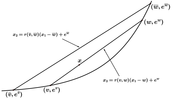
Figure 3. The subdomain $R_{4}$ and the geometric meaning of $v(x)$ and $w(x)$

Finally, here is our complete Bellman candidate. For $p>2$ and $C>C_{0}(p),$ let

(2.18) $$b_{p,C}(x)=\begin{cases}m_{1}(u)(x_{1}-u)+u^{p},&x\in R_{1},\vskip 12.0pt plus 4.0pt minus 4.0pt\par\\ q(\mkern 1.5mu\overline{\mkern-1.5muv\mkern-1.5mu}\mkern 1.5mu,\mkern 1.5mu\overline{\mkern-1.5muw\mkern-1.5mu}\mkern 1.5mu)\,(x_{1}-\mkern 1.5mu\overline{\mkern-1.5muw\mkern-1.5mu}\mkern 1.5mu)+\mkern 1.5mu\overline{\mkern-1.5muw\mkern-1.5mu}\mkern 1.5mu^{p}+\frac{m_{1}(\mkern 1.5mu\overline{\mkern-1.5muw\mkern-1.5mu}\mkern 1.5mu)-q(\mkern 1.5mu\overline{\mkern-1.5muv\mkern-1.5mu}\mkern 1.5mu,\mkern 1.5mu\overline{\mkern-1.5muw\mkern-1.5mu}\mkern 1.5mu)}{k(\mkern 1.5mu\overline{\mkern-1.5muw\mkern-1.5mu}\mkern 1.5mu)-r(\mkern 1.5mu\overline{\mkern-1.5muv\mkern-1.5mu}\mkern 1.5mu,\mkern 1.5mu\overline{\mkern-1.5muw\mkern-1.5mu}\mkern 1.5mu)}\big{(}x_{2}-r(\mkern 1.5mu\overline{\mkern-1.5muv\mkern-1.5mu}\mkern 1.5mu,\mkern 1.5mu\overline{\mkern-1.5muw\mkern-1.5mu}\mkern 1.5mu)(x_{1}-\mkern 1.5mu\overline{\mkern-1.5muw\mkern-1.5mu}\mkern 1.5mu)-e^{\mkern 1.5mu\overline{\mkern-1.5muw\mkern-1.5mu}\mkern 1.5mu}\big{)},&x\in R_{2},\vskip 12.0pt plus 4.0pt minus 4.0pt\par\\ m_{3}(u)(x_{1}-u)+(-u)^{p},&x\in R_{3},\vskip 12.0pt plus 4.0pt minus 4.0pt\par\\ q\big{(}v,w)\,(x_{1}-w)+w^{p},&x\in R_{4}.\end{cases}$$

Recall that here $u=u(x)$ is given by (2.2); $v=v(x)$ and $w=w(x)$ have just been defined in Lemma 2.6; $k$ is given by (2.1); $r$ and $q$ are given by (2.5); $m_{1}$ is given by (2.16); and $m_{3}$ is given by (2.17). In addition, $\mkern 1.5mu\overline{\mkern-1.5muw\mkern-1.5mu}\mkern 1.5mu$ was defined in Lemma 2.4 as the solution of equation (2.14), while $\mkern 1.5mu\overline{\mkern-1.5muv\mkern-1.5mu}\mkern 1.5mu$ was defined in the remark following that lemma as the unique solution of equation $F(v,\mkern 1.5mu\overline{\mkern-1.5muw\mkern-1.5mu}\mkern 1.5mu)=0$ with $F$ given by equation (2.7).

The next section presents the main theorem relating the candidate $b_{p,C}$ and the Bellman function $\boldsymbol{b}_{p,C}$ from (1.10).

3. The main Bellman theorem and a proof of the lower estimate

The following result is the principal ingredient in the proofs of Theorems 1.2 and 1.3.

Theorem 3.1.

If $p>2$ and $C>C_{0}(p),$ then

(3.1) $$\boldsymbol{b}_{p,C}=b_{p,C}\quad in\quad\Omega_{C}.$$

As is common, we split the proof of Theorem 3.1 in two parts: the so-called direct inequality $\boldsymbol{b}_{p,C}\geq b_{p,C}$ and its converse.

Lemma 3.2.

If $p>2$ and $C>C_{0}(p),$ then

(3.2) $$\boldsymbol{b}_{p,C}\geq b_{p,C}\quad in\quad\Omega_{C}.$$

Lemma 3.3.

If $p>2$ and $C>C_{0}(p),$ then

(3.3) $$\boldsymbol{b}_{p,C}\leq b_{p,C}\quad in\quad\Omega_{C}.$$

The proofs of Theorems  1.2 and 1.3 use only Lemma 3.2, which we prove in this section. For the sake of completeness, we will show that the infimum in the definition of the Bellman function is attained at every point in $\Omega_{C},$ and our candidate is in fact the Bellman function. This is done in Section 5 where we prove Lemma 3.3 .

The analog of Lemma 3.2 for $p\in[1,2]$ was proved in Section 5 of [8]. In fact, the proof given there did not depend on the specific range of $p$ used. Rather, its main ingredient was showing that $b_{p,C}$ is locally convex in $\Omega_{C},$ i.e., convex along every line segment contained in $\Omega_{C}.$ More precisely, the main result of Lemma 5.1 from [8] can be restated as follows.

Lemma 3.4 ([8]).

Fix $p>0$ and assume that for some $C(p)\geq 1$ there is a family of functions $\{b_{p,C}\}_{C\geq C(p)}$ satisfying the following conditions for each $C:$

1. $b_{p,C}$ is locally convex in $\Omega_{C};$

2. $b_{p,C}$ is continuous in $\Omega_{C};$

3. For each $x\in\Omega_{C},$

   $$\lim_{{\color[rgb]{0,0,0}c\searrow C}}b_{p,c}(x)=b_{p,C}(x);$$

4. For each $s\in\mathbb{R},$ $b_{p,C}(s,e^{s})=|s|^{p}.$

Then for all $C\geq C(p),$

$$\boldsymbol{b}_{p,C}\geq b_{p,C}\quad\text{in}\quad\Omega_{C}.$$

It is routine to check that conditions (2)-(4) are satisfied for $b_{p,C}$ from (2.18). Therefore, Lemma 3.2 will be proved once we have established the following result.

Lemma 3.5.

For $p>2$ and $C>C_{0}(p),$ the function $b_{p,C}$ is locally convex in $\Omega_{C}.$

Let us fix $p>2$ and $C>C_{0}(p)$ and through the end of this section write simply $b$ for $b_{p,C}.$ Before proving Lemma 3.5, let us collect several useful facts from earlier work. First, as explained in [10] and [8], showing that $b$ is locally convex in $\Omega_{C}$ is the same as showing that it is locally convex in each subdomain $R_{k}$ and that $b_{x_{2}}$ is increasing in $x_{2}$ across shared boundaries between subdomains. Second, in $R_{1}$ and $R_{3},$ $b$ has the form

$$b(x)=m(u)(x_{1}-u)+|u|^{p},$$

where $m$ stands for $m_{1}$ or $m_{3},$ respectively, and in each case satisfies the differential equation

(3.4) $$m^{\prime}(u)=\frac{1}{\xi}(m(u)-pu|u|^{p-2}),$$

and $u=u(x)$ is given by (2.2). As shown in [8], in such a case we have

(3.5) $$b_{x_{2}}=m^{\prime}(u)e^{-u}(1-\xi)$$

and also

(3.6) $$b_{x_{1}x_{1}}b_{x_{2}x_{2}}=b_{x_{1}x_{2}}^{2},\qquad\operatorname{sgn}b_{x_{2}x_{2}}=\operatorname{sgn}\big{(}m^{\prime}(u)-m^{\prime\prime}(u)\big{)}.$$

Therefore, to show that $b$ is locally convex in $R_{1}$ and $R_{3}$ we simply need to show that $m_{1}^{\prime}(u)-m_{1}^{\prime\prime}(u)>0$ in $R_{1}$ and $m_{3}^{\prime}(u)-m_{3}^{\prime\prime}(u)>0$ in $R_{3}.$

Proof of Lemma 3.5.

We first show local convexity of $b$ in each subdomain $R_{k}.$

In $R_{1},$ a direct computation gives

$$\frac{\xi^{2}}{p(p-1)}(m_{1}^{\prime}(u)-m_{1}^{\prime\prime}(u))e^{-u/\xi}=\xi u^{p-2}e^{-u/\xi}-(1-\xi)\int_{u}^{\infty}e^{-s/\xi}s^{p-2}\,ds=:H_{1}(u),$$

where $u\geq\mkern 1.5mu\overline{\mkern-1.5muw\mkern-1.5mu}\mkern 1.5mu.$ We have

$$H^{\prime}_{1}(u)=\xi u^{p-3}e^{-u/\xi}(p-2-u).$$

Therefore, $H_{1}$ is increasing for $u\in(0,p-2)$ and decreasing for $u>p-2.$ Since $H_{1}(u)\to 0$ as $u\to\infty,$ to show that $H_{1}(u)>0$ for $u\geq\mkern 1.5mu\overline{\mkern-1.5muw\mkern-1.5mu}\mkern 1.5mu,$ it suffices to show that $H_{1}(\mkern 1.5mu\overline{\mkern-1.5muw\mkern-1.5mu}\mkern 1.5mu)>0.$ This immediately follows by applying first (2.14) and then (2.10) with $w=\mkern 1.5mu\overline{\mkern-1.5muw\mkern-1.5mu}\mkern 1.5mu:$

$$(1-\xi)\int_{\mkern 1.5mu\overline{\mkern-1.5muw\mkern-1.5mu}\mkern 1.5mu}^{\infty}e^{-s/\xi}s^{p-2}\,ds=\frac{\xi e^{\mkern 1.5mu\overline{\mkern-1.5muw\mkern-1.5mu}\mkern 1.5mu(1-1/\xi)}}{p(p-1)}\,D(\mkern 1.5mu\overline{\mkern-1.5muw\mkern-1.5mu}\mkern 1.5mu)<\xi\mkern 1.5mu\overline{\mkern-1.5muw\mkern-1.5mu}\mkern 1.5mu^{p-2}e^{-\mkern 1.5mu\overline{\mkern-1.5muw\mkern-1.5mu}\mkern 1.5mu/\xi}.$$

Therefore, $b_{x_{2}x_{2}}>0$ in $R_{1}$ and so $b$ is locally convex in this subdomain.

In $R_{2},$ $b$ is affine and thus locally convex.

In $R_{3},$ we compute

$$\frac{\xi^{2}}{p(p-1)}(m_{3}^{\prime}(u)-m_{3}^{\prime\prime}(u))e^{-u/\xi}$$

$$\qquad=\xi(-u)^{p-2}e^{-u/\xi}-(1-\xi)\Big{(}\int_{u}^{\mkern 1.5mu\overline{\mkern-1.5muv\mkern-1.5mu}\mkern 1.5mu}e^{-s/\xi}(-s)^{p-2}\,ds+e^{(\mkern 1.5mu\overline{\mkern-1.5muw\mkern-1.5mu}\mkern 1.5mu-\mkern 1.5mu\overline{\mkern-1.5muv\mkern-1.5mu}\mkern 1.5mu)(1/\xi-1)}\int_{\mkern 1.5mu\overline{\mkern-1.5muw\mkern-1.5mu}\mkern 1.5mu}^{\infty}e^{-s/\xi}s^{p-2}\,ds\Big{)}$$

$$\qquad=:H_{3}(u),$$

where $u\leq\mkern 1.5mu\overline{\mkern-1.5muv\mkern-1.5mu}\mkern 1.5mu.$ We have

$$H^{\prime}_{3}(u)=\xi(-u)^{p-3}e^{-u/\xi}(u-p+2)<0,$$

and so to show that $H_{3}(u){\color[rgb]{0,0,0}>}0,$ it is enough to show that $H_{3}(\mkern 1.5mu\overline{\mkern-1.5muv\mkern-1.5mu}\mkern 1.5mu){\color[rgb]{0,0,0}>}0.$ Similarly to the case of $H_{1},$ this follows from an application of (2.14) and then of (2.9) with $v=\mkern 1.5mu\overline{\mkern-1.5muv\mkern-1.5mu}\mkern 1.5mu:$

$$(1-\xi)e^{(\mkern 1.5mu\overline{\mkern-1.5muw\mkern-1.5mu}\mkern 1.5mu-\mkern 1.5mu\overline{\mkern-1.5muv\mkern-1.5mu}\mkern 1.5mu)(1/\xi-1)}\int_{\mkern 1.5mu\overline{\mkern-1.5muw\mkern-1.5mu}\mkern 1.5mu}^{\infty}e^{-s/\xi}s^{p-2}\,ds=\frac{\xi e^{-\mkern 1.5mu\overline{\mkern-1.5muv\mkern-1.5mu}\mkern 1.5mu(1/\xi-1)}}{p(p-1)}\,D(\mkern 1.5mu\overline{\mkern-1.5muw\mkern-1.5mu}\mkern 1.5mu){\color[rgb]{0,0,0}<}\xi(-\mkern 1.5mu\overline{\mkern-1.5muv\mkern-1.5mu}\mkern 1.5mu)^{p-2}e^{-\mkern 1.5mu\overline{\mkern-1.5muv\mkern-1.5mu}\mkern 1.5mu/\xi}.$$

Thus, $b$ is locally convex in $R_{3}.$

Let us state the result for $R_{4}$ separately.

Lemma 3.6.

$b$ is convex in $R_{4}.$

Proof.

In $R_{4},$ $b$ is given by

$$b(x)=q(v,w)(x_{1}-w)+f(w),\qquad x_{2}=r(v,w)(x_{1}-w)+g(w),$$

where, as in the proof of Lemma 2.3, we write $f(w)=w^{p}$ and $g(w)=e^{w}.$ Let us also, as we did there, use the prime to indicate the total derivative with respect to $w.$

To show that $b$ is convex, we show that $b_{x_{1}x_{1}}b_{x_{2}x_{2}}=b_{x_{1}x_{2}}^{2}$ and $b_{x_{2}x_{2}}>0$ in the interior of $R_{4}.$ Differentiating gives

$$w_{x_{1}}=\frac{-r}{r^{\prime}(x_{1}-w)-r+g^{\prime}},\qquad w_{x_{2}}=\frac{1}{r^{\prime}(x_{1}-w)-r+g^{\prime}},$$

and

$$b_{x_{1}} =\big{[}q^{\prime}(x_{1}-w)-q+f^{\prime}\big{]}w_{x_{1}}+q=-r\,\frac{q^{\prime}(x_{1}-w)-q+f^{\prime}}{r^{\prime}(x_{1}-w)-r+g^{\prime}}+q=-rD+q,$$

where we used (2.11). Similarly,

(3.7) $${\color[rgb]{0,0,0}b_{x_{2}}=\big{[}q^{\prime}(x_{1}-w)-q+f^{\prime}\big{]}w_{x_{2}}=\frac{q^{\prime}(x_{1}-w)-q+f^{\prime}}{r^{\prime}(x_{1}-w)-r+g^{\prime}}=D.}$$

Therefore,

$$b_{x_{1}x_{1}}=-rD^{\prime}w_{x_{1}},\quad b_{x_{1}x_{2}}=-rD^{\prime}w_{x_{2}},\quad b_{x_{2}x_{2}}=D^{\prime}w_{x_{2}},$$

and, since, $w_{x_{1}}=-rw_{x_{2}},$ we see that $b_{x_{1}x_{1}}b_{x_{2}x_{2}}=b_{x_{1}x_{2}}^{2}.$

Furthermore, since by Lemma 2.3, $D^{\prime}>0$ and since it is clear from geometry that $w_{x_{2}}>0,$ we have $b_{x_{2}x_{2}}>0,$ which completes the proof. ∎

To finish the proof of Lemma 3.5, we need to verify that $b_{x_{2}}$ is increasing in $x_{2}$ across boundaries between subdomains. We can write this requirement symbolically as:

$$b_{x_{2}}\Big{|}_{R_{1},u=\mkern 1.5mu\overline{\mkern-1.5muw\mkern-1.5mu}\mkern 1.5mu}\leq b_{x_{2}}\Big{|}_{R_{2}},\qquad b_{x_{2}}\Big{|}_{R_{4},w=\mkern 1.5mu\overline{\mkern-1.5muw\mkern-1.5mu}\mkern 1.5mu}\leq b_{x_{2}}\Big{|}_{R_{2}},\qquad b_{x_{2}}\Big{|}_{R_{2}}\leq b_{x_{2}}\Big{|}_{R_{3},u=\mkern 1.5mu\overline{\mkern-1.5muv\mkern-1.5mu}\mkern 1.5mu}.$$

In fact, all three statements hold with equality (which implies that $b$ is of class $C^{1}$ in the interior of $\Omega_{C},$ though we will not use this fact).

From (3.7), we have $b_{x_{2}}{\color[rgb]{0,0,0}\big{|}_{R_{4},w=\mkern 1.5mu\overline{\mkern-1.5muw\mkern-1.5mu}\mkern 1.5mu}}=D(\mkern 1.5mu\overline{\mkern-1.5muw\mkern-1.5mu}\mkern 1.5mu).$ Using, in order, (3.5), (3.4), (2.16), integration by parts, and (2.14) gives:

(3.8) $$b_{x_{2}}\Big{|}_{R_{1},u=\mkern 1.5mu\overline{\mkern-1.5muw\mkern-1.5mu}\mkern 1.5mu}=m_{1}^{\prime}(\mkern 1.5mu\overline{\mkern-1.5muw\mkern-1.5mu}\mkern 1.5mu)e^{-\mkern 1.5mu\overline{\mkern-1.5muw\mkern-1.5mu}\mkern 1.5mu}(1-\xi)=\frac{1}{\xi}(1-\xi)p(p-1)e^{\mkern 1.5mu\overline{\mkern-1.5muw\mkern-1.5mu}\mkern 1.5mu(1/\xi-1)}\int_{\mkern 1.5mu\overline{\mkern-1.5muw\mkern-1.5mu}\mkern 1.5mu}^{\infty}s^{p-2}e^{-s/\xi}\,ds=D(\mkern 1.5mu\overline{\mkern-1.5muw\mkern-1.5mu}\mkern 1.5mu).$$

A very similar calculation, but using (2.17) in place of (2.16), gives $b_{x_{2}}\big{|}_{R_{3},u=\mkern 1.5mu\overline{\mkern-1.5muv\mkern-1.5mu}\mkern 1.5mu}=D(\mkern 1.5mu\overline{\mkern-1.5muw\mkern-1.5mu}\mkern 1.5mu).$

Finally,

$$b_{x_{2}}\Big{|}_{R_{2}}=\frac{m_{1}(\mkern 1.5mu\overline{\mkern-1.5muw\mkern-1.5mu}\mkern 1.5mu)-q(\mkern 1.5mu\overline{\mkern-1.5muv\mkern-1.5mu}\mkern 1.5mu,\mkern 1.5mu\overline{\mkern-1.5muw\mkern-1.5mu}\mkern 1.5mu)}{k(\mkern 1.5mu\overline{\mkern-1.5muw\mkern-1.5mu}\mkern 1.5mu)-r(\mkern 1.5mu\overline{\mkern-1.5muv\mkern-1.5mu}\mkern 1.5mu,\mkern 1.5mu\overline{\mkern-1.5muw\mkern-1.5mu}\mkern 1.5mu)}.$$

By (3.4) and (3.8),

$$m_{1}(\mkern 1.5mu\overline{\mkern-1.5muw\mkern-1.5mu}\mkern 1.5mu)=\xi m_{1}^{\prime}(\mkern 1.5mu\overline{\mkern-1.5muw\mkern-1.5mu}\mkern 1.5mu)+p\mkern 1.5mu\overline{\mkern-1.5muw\mkern-1.5mu}\mkern 1.5mu^{p-1}=\frac{\xi}{1-\xi}\,e^{\mkern 1.5mu\overline{\mkern-1.5muw\mkern-1.5mu}\mkern 1.5mu}D(\mkern 1.5mu\overline{\mkern-1.5muw\mkern-1.5mu}\mkern 1.5mu)+p\mkern 1.5mu\overline{\mkern-1.5muw\mkern-1.5mu}\mkern 1.5mu^{p-1}.$$

Therefore,

$$b_{x_{2}}\Big{|}_{R_{2}}=\frac{\frac{\xi}{1-\xi}\,e^{\mkern 1.5mu\overline{\mkern-1.5muw\mkern-1.5mu}\mkern 1.5mu}D(\mkern 1.5mu\overline{\mkern-1.5muw\mkern-1.5mu}\mkern 1.5mu)+p\mkern 1.5mu\overline{\mkern-1.5muw\mkern-1.5mu}\mkern 1.5mu^{p-1}-q(\mkern 1.5mu\overline{\mkern-1.5muv\mkern-1.5mu}\mkern 1.5mu,\mkern 1.5mu\overline{\mkern-1.5muw\mkern-1.5mu}\mkern 1.5mu)}{\frac{1}{1-\xi}\,e^{\mkern 1.5mu\overline{\mkern-1.5muw\mkern-1.5mu}\mkern 1.5mu}-r(\mkern 1.5mu\overline{\mkern-1.5muv\mkern-1.5mu}\mkern 1.5mu,\mkern 1.5mu\overline{\mkern-1.5muw\mkern-1.5mu}\mkern 1.5mu)}=\frac{\frac{\xi}{1-\xi}\,e^{\mkern 1.5mu\overline{\mkern-1.5muw\mkern-1.5mu}\mkern 1.5mu}D(\mkern 1.5mu\overline{\mkern-1.5muw\mkern-1.5mu}\mkern 1.5mu)+\big{(}e^{\mkern 1.5mu\overline{\mkern-1.5muw\mkern-1.5mu}\mkern 1.5mu}-r(\mkern 1.5mu\overline{\mkern-1.5muv\mkern-1.5mu}\mkern 1.5mu,\mkern 1.5mu\overline{\mkern-1.5muw\mkern-1.5mu}\mkern 1.5mu)\big{)}D(\mkern 1.5mu\overline{\mkern-1.5muw\mkern-1.5mu}\mkern 1.5mu)}{\frac{1}{1-\xi}\,e^{\mkern 1.5mu\overline{\mkern-1.5muw\mkern-1.5mu}\mkern 1.5mu}-r(\mkern 1.5mu\overline{\mkern-1.5muv\mkern-1.5mu}\mkern 1.5mu,\mkern 1.5mu\overline{\mkern-1.5muw\mkern-1.5mu}\mkern 1.5mu)}=D(\mkern 1.5mu\overline{\mkern-1.5muw\mkern-1.5mu}\mkern 1.5mu).$$

The proof is complete. ∎

We are now in a position to prove the main theorems stated in Section 1.

4. Proofs of Theorems 1.2 and 1.3

We will need two auxiliary results from [8].

For $p>0,$ let

$$\omega(p)=\left[\frac{p}{e}\Big{(}\Gamma(p)-\int_{0}^{1}t^{p-1}e^{t}\,dt\Big{)}+1\right]^{1/p}.$$

Lemma 4.1 ([8]).

Let $\varphi_{0}(t)=\log(1/t),~{}t\in(0,1).$ Then

(4.1) $$\varepsilon_{\varphi_{0}}=1,\qquad\varepsilon_{-\varphi_{0}}=\infty.$$

If $p\geq 1,$ then

(4.2) $$\|\varphi_{0}\|_{{\rm BMO}^{p}((0,1))}=\omega(p).$$

Consequently,

(4.3) $$\varepsilon_{0}(p)\leq\omega(p).$$

Lemma 4.2 ([8]).

Let $\varphi$ be a non-constant ${\rm BMO}$ function. For $\varepsilon\in[0,\varepsilon_{\varphi}),$ let $F(\varepsilon)=[e^{\varepsilon\varphi}]_{A_{\infty}}.\!\!$ Then $F$ is a strictly increasing, continuous function on $[0,\varepsilon_{\varphi}),$ and $\lim_{\varepsilon\to\varepsilon_{\varphi}}F(\varepsilon)\!=\!\infty.$

Proof of Theorem 1.2.

We use Theorem 1.4 with $b_{C}=b_{p,C}$ given by formula 2.18. By Lemma 3.2, $b_{C}\leq\boldsymbol{b}_{p,C},$ as required.

We need to compute $b_{p,C}(0,C).$ Note that by Lemma 2.4, $\mkern 1.5mu\overline{\mkern-1.5muw\mkern-1.5mu}\mkern 1.5mu<\xi,$ and, thus, $\mkern 1.5mu\overline{\mkern-1.5muv\mkern-1.5mu}\mkern 1.5mu>-\mkern 1.5mu\overline{\mkern-1.5muw\mkern-1.5mu}\mkern 1.5mu>-\xi$ by Lemma 2.2. Therefore, the point $(0,C)$ is in subdomain $R_{3}$ and, since $u(0,C)=-\xi,$

$$b_{p,C}(0,C)=m_{3}(-\xi)\xi+\xi^{p}.$$

Now, $m_{3}(-\xi)$ is given by (2.17):

$$m_{3}(-\xi)=-\frac{p}{\xi}\,e^{-1}\int_{-\xi}^{\mkern 1.5mu\overline{\mkern-1.5muv\mkern-1.5mu}\mkern 1.5mu}(-s)^{p-1}e^{-s/\xi}\,ds+e^{(-\xi-\mkern 1.5mu\overline{\mkern-1.5muv\mkern-1.5mu}\mkern 1.5mu)/\xi}\left(e^{\mkern 1.5mu\overline{\mkern-1.5muv\mkern-1.5mu}\mkern 1.5mu-\mkern 1.5mu\overline{\mkern-1.5muw\mkern-1.5mu}\mkern 1.5mu}\big{(}m_{1}(\mkern 1.5mu\overline{\mkern-1.5muw\mkern-1.5mu}\mkern 1.5mu)-p\mkern 1.5mu\overline{\mkern-1.5muw\mkern-1.5mu}\mkern 1.5mu^{p-1}\big{)}-p(-\mkern 1.5mu\overline{\mkern-1.5muv\mkern-1.5mu}\mkern 1.5mu)^{p-1}\right).$$

By Lemma 2.4, $\mkern 1.5mu\overline{\mkern-1.5muw\mkern-1.5mu}\mkern 1.5mu\in(0,c_{2})$ with $c_{2}\to 0$ as $\xi\to 1.$ By Lemma 2.2, $\mkern 1.5mu\overline{\mkern-1.5muv\mkern-1.5mu}\mkern 1.5mu\in(-\mkern 1.5mu\overline{\mkern-1.5muw\mkern-1.5mu}\mkern 1.5mu,0).$ Therefore,

$$\lim_{\xi\to 1}\mkern 1.5mu\overline{\mkern-1.5muv\mkern-1.5mu}\mkern 1.5mu=\lim_{\xi\to 1}\mkern 1.5mu\overline{\mkern-1.5muw\mkern-1.5mu}\mkern 1.5mu=0$$

and

$$\lim_{C\to\infty}b_{p,C}(0,C)=\lim_{\xi\to 1}\big{(}m_{3}(-\xi)\xi+\xi^{p}\big{)}=-\frac{p}{e}\int_{-1}^{0}(-s)^{p-1}e^{-s}\,ds+e^{-1}m_{1}(0)+1=\omega^{p}(p),$$

where we used (2.16), whereby $m_{1}(0)=p\Gamma(p).$

Hence, by Theorem 1.4, $\varepsilon_{0}(p)\geq\omega(p),$ and Lemma 4.1 now finishes the proof. ∎

The proof of Theorem 1.3 below is a variation of the argument for Corollary 1.5 in [8]; the proof of sharpness, using function $\varphi_{0}$ from Lemma 4.1, is exactly the same and we omit it.

Proof of Theorem 1.3.

Take any $\varphi\in{\rm BMO}(Q).$ Without loss of generality, assume $\varepsilon_{\varphi}<\infty.$ For $\varepsilon\in[0,\varepsilon_{\varphi}),$ let $F(\varepsilon)=[e^{\varepsilon\varphi}]_{A_{\infty}(Q)}.$ By Lemma 4.2, for sufficiently large $\varepsilon$ we have $F(\varepsilon)\geq C_{0}(p).$ Therefore, for any subinterval $J$ of $Q,$

$$\langle|\varepsilon\varphi-\langle\varepsilon\varphi\rangle_{{}_{\scriptstyle J}}|^{p}\rangle_{{}_{\scriptstyle J}}\geq\boldsymbol{b}_{p,F(\varepsilon)}\big{(}0,\langle e^{\varepsilon\varphi-\langle\varepsilon\varphi\rangle_{{}_{\scriptscriptstyle J}}}\rangle_{{}_{\scriptstyle J}}\big{)}\geq b_{p,F(\varepsilon)}\big{(}0,\langle e^{\varepsilon\varphi-\langle\varepsilon\varphi\rangle_{{}_{\scriptscriptstyle J}}}\rangle_{{}_{\scriptstyle J}}\big{)}.$$

Take a sequence $\{J_{n}\}$ such that $\langle e^{\varepsilon\varphi-\langle\varepsilon\varphi\rangle_{{}_{\scriptscriptstyle J_{n}}}}\rangle_{{}_{\scriptstyle J_{n}}}\to F(\varepsilon).$ Since the left-hand side is bounded from above by $\varepsilon^{p}\|\varphi\|^{p}_{{\rm BMO}^{p}(Q)},$ we have

$$\varepsilon^{p}\|\varphi\|^{p}_{{\rm BMO}^{p}(Q)}\geq b_{p,F(\varepsilon)}\big{(}0,F(\varepsilon)\big{)}.$$

Now, take $\varepsilon\to\varepsilon_{\varphi}$ (and, thus, $F(\varepsilon)\to\infty).$ This gives

$$\varepsilon^{p}_{\varphi}\|\varphi\|^{p}_{{\rm BMO}^{p}(Q)}\geq\varepsilon^{p}_{0}(p).$$

Take any $f\in L^{\infty}(Q),$ then $\varepsilon_{\varphi-f}={\color[rgb]{0,0,0}\varepsilon_{\varphi}}.$ Thus, we can replace $\varphi$ with $\varphi-f$ above, which gives

$$\|\varphi-f\|_{{\rm BMO}^{p}(Q)}\geq\frac{\varepsilon_{0}(p)}{\varepsilon_{\varphi}}.$$

The same inequality holds with $\varphi$ replaced with $-\varphi,$ and it remains to take the infimum over $f\in L^{\infty}(Q)$ on the left. ∎

5. Optimizers and the converse inequality

In this section, we complete the proof of Theorem 3.1 by proving Lemma 3.3. To that end, we present a set of special test functions on the interval $(0,1)$ that realize the infimum in definition (1.10) of the Bellman function $\boldsymbol{b}_{p,C}.$

Without loss of generality assume $C>1.$ Let $Q=(0,1).$ Recall the Bellman candidate $b_{p,C}$ given by formula (2.18). For $x\in\Omega_{C},$ we say that a function $\varphi_{x}$ on $Q$ is an optimizer for $b_{p,C}$ at $x$ if

(5.1) $$\varphi_{x}\in E_{x,C,Q}\quad\text{and}\quad\langle|\varphi_{x}|^{p}\rangle_{{}_{\scriptstyle Q}}=b_{p,C}(x),$$

where the set of test functions $E_{x,C,Q}$ is defined by (1.9). Observe that if we have such a function $\varphi_{x}$ for all $x\in\Omega_{C},$ then

$$b_{p,C}(x)=\langle|\varphi|^{p}\rangle_{{}_{\scriptstyle Q}}\geq\boldsymbol{b}_{p,C}(x),$$

which is the statement of Lemma 3.3.

Our optimizers $\varphi_{x}$ will have different forms depending on the location of $x$ in $\Omega_{C}.$ Specifically, we will have a different optimizer for each of the four subdomains $R_{k}$ of $\Omega_{C}$ defined by formula (1.8) and pictured in Figure 2. We do not discuss the construction of these optimizers, but simply give formulas for them. A reader interested in where they come from is invited to consult papers [10] and [3], where a number of similar constructions are carried out in the context of ${\rm BMO}^{2}.$

For each $x\in R_{1},$ let

(5.2) $$\varphi_{x}(t)=u+\xi\log\big{(}{\textstyle\frac{\alpha}{t}}\big{)}\chi_{(0,\alpha)}(t),$$

where $u=u(x)$ is defined by (2.2) and we set

(5.3) $$\alpha=\frac{x_{1}-u}{\xi}.$$

(This optimizer was defined in Section 5 of [8] under the name $\varphi^{+}_{x}$.)

Now consider the subdomain $R_{2}.$ Let us give names to its four corners, clockwise from top right:

$$X=(\mkern 1.5mu\overline{\mkern-1.5muw\mkern-1.5mu}\mkern 1.5mu+\xi,e^{\mkern 1.5mu\overline{\mkern-1.5muw\mkern-1.5mu}\mkern 1.5mu+\xi}),\qquad Y=(\mkern 1.5mu\overline{\mkern-1.5muw\mkern-1.5mu}\mkern 1.5mu,e^{\mkern 1.5mu\overline{\mkern-1.5muw\mkern-1.5mu}\mkern 1.5mu}),\qquad Z=(\mkern 1.5mu\overline{\mkern-1.5muv\mkern-1.5mu}\mkern 1.5mu,e^{\mkern 1.5mu\overline{\mkern-1.5muv\mkern-1.5mu}\mkern 1.5mu}),\qquad W=(\mkern 1.5mu\overline{\mkern-1.5muv\mkern-1.5mu}\mkern 1.5mu+\xi,e^{\mkern 1.5mu\overline{\mkern-1.5muv\mkern-1.5mu}\mkern 1.5mu+\xi}).$$

We already know the optimizers for the points $X,$ $Y,$ and $Z:$ the first comes from formula (5.2) (which applies since $X\in R_{1}\cap R_{2}$) with $\alpha=1;$ the other two are trivial, since for each $x\in\Gamma_{1},$ the set $E_{x,C,Q}$ contains only one element — the constant function $\varphi(t)=x_{1}.$ Therefore, we define, for all $t\in Q,$

$$\varphi_{X}(t)=\xi\log\big{(}{\textstyle\frac{1}{t}}\big{)},\qquad\varphi_{Y}(t)=\mkern 1.5mu\overline{\mkern-1.5muw\mkern-1.5mu}\mkern 1.5mu,\qquad\varphi_{Z}(t)=\mkern 1.5mu\overline{\mkern-1.5muv\mkern-1.5mu}\mkern 1.5mu.$$

We now use these three optimizers to define $\varphi_{x}$ for every $x\in R_{2}.$ Observe that $R_{2}$ is contained in the triangle with the vertices $X,$ $Y,$ $Z.$ This means that every $x$ in $R_{2}$ has a unique representation as a convex combination of these three points. Thus, there are non-negative numbers $\alpha_{1},$ $\alpha_{2},$ and $\alpha_{3}$ such that $\alpha_{1}+\alpha_{2}+\alpha_{3}=1$ and

(5.4) $$x=\alpha_{1}X+\alpha_{2}Y+\alpha_{3}Z.$$

To obtain $\varphi_{x},$ we concatenate $\varphi_{X},$ $\varphi_{Y},$ and $\varphi_{Z}$ in the appropriate proportion:

$$\varphi_{x}(t)=\varphi_{X}\big{(}{\textstyle\frac{t}{\alpha_{1}}}\big{)}\chi_{(0,\alpha_{1})}(t)+\varphi_{Y}\big{(}{\textstyle\frac{t-\alpha_{1}}{\alpha_{2}}}\big{)}\chi_{(\alpha_{1},\alpha_{1}+\alpha_{2})}(t)+\varphi_{Z}\big{(}{\textstyle\frac{t-\alpha_{1}-\alpha_{2}}{\alpha_{3}}}\big{)}\chi_{(\alpha_{1}+\alpha_{2},1)}(t),$$

or, equivalently,

(5.5) $$\varphi_{x}(t)=\mkern 1.5mu\overline{\mkern-1.5muw\mkern-1.5mu}\mkern 1.5mu\,\chi_{(0,\alpha_{1}+\alpha_{2})}(t)+\xi\log\big{(}{\textstyle\frac{{\alpha_{1}}}{t}}\big{)}\chi_{(0,\alpha_{1})}(t)+\mkern 1.5mu\overline{\mkern-1.5muv\mkern-1.5mu}\mkern 1.5mu\,\chi_{(\alpha_{1}+\alpha_{2},1)}(t),$$

with $\alpha_{k}=\alpha_{k}(x)$ defined by (5.4).

This formula applies, in particular, to the fourth corner of $R_{2},$ i.e., the point $W.$ Since that point also lies in the subdomain $R_{3},$ the optimizer $\varphi_{W}$ will enter into the definition of $\varphi_{x}$ for all $x\in R_{3}.$ Specifically, for each such $x$ we set:

(5.6) $$\varphi_{x}(t)=\varphi_{W}\big{(}{\textstyle\frac{t}{\tau\alpha}}\big{)}\chi_{(0,\tau\alpha)}(t)+\xi\log\big{(}{\textstyle\frac{\alpha}{t}}\big{)}\chi_{(\tau\alpha,\alpha)}(t)+u\chi_{(\tau\alpha,1)}(t).$$

Here, $u$ is defined by (2.2), $\alpha$ is defined by (5.3), and we also set

(5.7) $$\tau=e^{(u-\mkern 1.5mu\overline{\mkern-1.5muv\mkern-1.5mu}\mkern 1.5mu)/\xi}.$$

It remains to define $\varphi_{x}$ when $x\in R_{4}.$ Recall the two auxiliary functions $v=v(x)$ and $w=w(x)$ defined by Lemma 2.6 (see Figure 3). Every point $x\in R_{4}\setminus\Gamma_{1}$ lies on the line segment connecting the points $(v,e^{v})$ and $(w,e^{w}).$ Accordingly, we define $\varphi_{x}$ to be the appropriate concatenation of the two consant optimizers corresponding to those points:

(5.8) $$\varphi_{x}(t)=w\,\chi_{(0,\beta)}(t)+v\,\chi_{(\beta,1)}(t),$$

where we set

(5.9) $$\beta=\frac{x_{1}-v}{w-v}.$$

We now state the main lemma, which immediately yields Lemma 3.3

Lemma 5.1.

Let $\varphi_{x}$ be defined by (5.2) and (5.3) for $x\in R_{1};$ by (5.4) and (5.5) for $x\in R_{2};$ by (5.6), (5.3), and (5.7) for $x\in R_{3};$ and by (5.8) and (5.9) for $x\in R_{4}.$ Then $\varphi_{x}$ is an optimizer for $b_{p,C}$ at every $x\in\Omega_{C}.$

Remark 5.2.

If a point $x$ lies on a boundary shared by two subdomains, $\varphi_{x}$ seems to be defined by two different formulas. However, as is easy to check, in all cases above, such two formulas give exactly the same function.

The proof of this lemma is very similar to the proof of Lemma 5.2 from [8] and we leave it to the reader.

References

- [1] J. Garnett, P. Jones. The distance in to Annals of Mathematics. Vol. 108 (1978), pp. 373–393
- [2] P. Ivanishvili, N. Osipov, D. Stolyarov, V. Vasyunin, P. Zatitskiy, On Bellman function for extremal problems in BMO. C. R. Math. Acad. Sci. Paris 350 (2012), No. 11-12, pp. 561–564
- [3] P. Ivanishvili, N. Osipov, D. Stolyarov, V.Vasyunin, P. Zatitskiy. Bellman function for extremal problems in BMO. To appear in Transactions of the AMS, pp. 1-91. Available at arXiv:1205.7018
- [4] P. Ivanishvili, D. Stolyarov, V.Vasyunin, P. Zatitskiy. Bellman functions on general non-convex planar domains. In preparation.
- [5] F. John, L. Nirenberg. On functions of bounded mean oscillation. Comm. Pure Appl. Math. 14 1961, pp. 415–426
- [6] A. Korenovskii. The connection between mean oscillations and exact exponents of summability of functions. Math. USSR-Sb., Vol. 71 (1992), no. 2, pp. 561–567
- [7] A. Lerner. The John–Nirenberg inequality with sharp constants. C. R. Math. Acad. Sci. Paris, Vol. 351 (2013), no. 11-12, pp. 463–466
- [8] L. Slavin. The John–Nirenberg constant of Submitted. Available at arXiv:1506.04969
- [9] L. Slavin, V. Vasyunin. Sharp results in the integral-form John–Nirenberg inequality. Trans. Amer. Math. Soc., Vol. 363, No. 8 (2011), pp. 4135–4169
- [10] L. Slavin, V. Vasyunin. Sharp estimates on BMO. Indiana Univ. Math. J., Vol. 61 (2012), No. 3, pp. 1051–1110
- [11] D. Stolyarov, P. Zatitskiy. Theory of locally concave functions and its applications to sharp estimates of integral functionals. Submitted. Available at arXiv:1412.5350v1
- [12] V. Vasyunin, A. Volberg. Sharp constants in the classical weak form of the John–Nirenberg inequality. Proc. Lond. Math. Soc. (3), Vol. 108 (2014), No. 6, pp. 1417–1434