Photoproduction of K$\Lambda$ on the proton

Abstract

Kaon photoproduction on the proton is studied in the resonance region using an isobar model. The higher-spin nucleon (3/2 and 5/2) and hyperon (3/2) resonances were included in the model utilizing the consistent formalism by Pascalutsa, and they were found to play an important role in data description. The spin-1/2 and spin-3/2 hyperon resonances in combination with the Born terms contribute significantly to the background part of the amplitude. Various forms of the hadron form factor were considered in the construction, and the dipole and multidipole forms were selected as those most suitable for the data description. Model parameters were fitted to new experimental data from CLAS, LEPS, and GRAAL collaborations and two versions of the model, BS1 and BS2, were chosen. Both models provide a good overall description of the data for the center-of-mass energies from the threshold up to 2.4 GeV. Predicted cross sections of the models at very small kaon angles being consistent with results of the Saclay-Lyon model indicate that the models could be also successful in predicting the hypernucleus production cross sections. Although kaon photoproduction takes place in the third-resonance region with many resonant states, the total number of included resonances, 15 and 16, is quite moderate and it is comparable with numbers of resonances in other models. The set of chosen nucleon resonances overlaps well with the set of the most probable contributing states determined in the Bayesian analysis with the Regge-plus-resonance model. Particularly, we confirm that the missing resonances $P_{13}(1900)$ and $D_{13}(1875)$ do play an important role in the description of data. However, the spin-1/2 state $P_{11}(1880)$ included in the Bayesian analysis was replaced in our analysis with the near-mass spin-5/2 state $N^{*}(1860)$, recently considered by the Particle Data Group.

I Introduction

The investigation of kaon-hyperon photo- and electroproduction from nucleons in the nucleon resonance region provides important information about the baryon resonance spectrum and interactions in hyperon-nucleon systems arising from QCD. Besides studying the reaction mechanism, one can learn more about the existence and properties of the “missing” resonances that are predicted by the quark models CapRob00 ; Bonn but that are weakly coupled to the $\pi$N final state and therefore are not seen in the pion production or $\pi$N scattering processes. A correct description of the elementary $\Lambda$-production process is also important for getting reliable predictions of the excitation spectra for production of $\Lambda$ hypernuclei HProd ; ByMa .

Numerous theoretical studies of the hyperon production have been performed over the past decades. The analyses before 2004, however, suffered from a lack of high-quality experimental data, see e.g., Refs. AS ; SL ; SLA ; Jan01A ; Jan01B ; Jan02 ; WJC ; models and references therein. The situation changed significantly after new high-duty-factor accelerators, providing good quality high-current polarized continuous beams, were constructed in Jefferson Lab (CEBAF) and Bonn University (ELSA). Number of good quality data, especially from the CLAS CLAS05 ; CLAS10 , LEPS LEPS , GRAAL GRAAL , and SAPHIR SAPHIR collaborations, rose by more than a factor of 10 which revived interest in modeling the process Giessen ; JDiaz ; Anisovich ; Borasoy ; GentRPR07 ; MartSu ; Mart ; Maxwell . Now various response functions are accessible and measured with a good level of precision in the energy region from the threshold up to 2.8 GeV, which allows us to perform more rigorous tests of theoretical models and improve our understanding of the elementary process.

The models of $\gamma\rm p\longrightarrow K^{+}\Lambda$ that are in a close connection with QCD are based on quark degrees of freedom ZpL95 ; LLP95 ; FHZ91 . These quark models need a relatively small number of parameters and assume explicitly a spatial-extended structure of the baryons which was found to be important for a reasonable description of the photoproduction data LLP95 . Contributions of baryon resonances in the intermediate state then arise naturally from effects of excited states of the quark system. Alternative approaches to description of the production process at low energies assume hadrons as appropriate effective degrees of freedom. Calculations grounded in an effective Lagrangian containing interacting meson, baryon and electromagnetic fields provide us with a valuable tool for analysis of experimental data. As there is no explicit connection to QCD, the number of parameters in the models is related to the number of resonances included in the calculations and is, therefore, relatively large for the kaon production SL ; SLA ; Jan01A ; Jan01B ; Jan02 ; MartSu . The short-range physics manifesting itself via a spatial structure of hadrons can be simulated by a form factor introduced in the interaction vertex. This, however, brings another ambiguity into the model: the forms and parameters of the form factors, which have to be fixed in a data analysis.

In some models the concept of chiral symmetry is utilized to include the pseudoscalar mesons as the Goldstone bosons in the chiral quark model ZpL95 or to build up a chiral effective meson-baryon Lagrangian in the gauge-invariant chiral unitary model Borasoy . Attempts were also made to calculate the kaon-hyperon photoproduction processes in the threshold region in the framework of the chiral perturbation theory Chpt .

In the hadrodynamical approach, the production channels are coupled by the meson-baryon interaction in the final state and should be, therefore, treated simultaneously to maintain unitarity. In the coupled-channel approaches Giessen ; JDiaz ; Anisovich ; Borasoy , the rescattering effects in the meson-baryon final-state system are included, but the models face the problem of missing experimental information on some transition amplitudes, e.g., ${\rm K^{+}}\Lambda\longrightarrow{\rm K^{+}}\Lambda$. Considerable simplification originates from neglecting the rescattering effects in the formalism, assuming that their influence on the results is included to some extent by means of effective values of the coupling constants fitted to experimental data. This simplifying assumption was adopted in many single-channel isobar models, e.g., Saclay-Lyon (SL) SL ; SLA , Kaon-MAID (KM) KM , and Gent-Isobar Jan01A ; Jan01B ; Jan02 . Unitarity corrections in the single-channel approach can be included by energy-dependent widths in the resonance propagators KM . Since the early work of Thom Thom , the isobar models were among the first models capable of describing the kaon photoproduction in the resonance region.

The kaon production takes place in the third-resonance region, with many possible nucleon and hyperon higher-spin states coupling to the kaon-hyperon channels. Therefore, the contributions of higher-spin baryon resonances are particularly important in the isobar models. The theoretical description of the interacting baryon fields with a spin higher than 1/2 causes problems due to the presence of nonphysical lower-spin components in the Rarita-Schwinger field Benm . Some prescriptions for the propagator and vertexes had to be adopted to handle the higher-spin problem; see, e.g., Refs. SL ; SLA for the case of spin-3/2 nucleon resonances. This prescription, however, requires fixing additional free parameters in the Lagrangian, the off-shell parameters SLA ; Jan01A ; Jan01B ; Jan02 . Moreover, the prescription used in Ref. SL did not allow inclusion of the hyperon resonances with spin 3/2 due to the terms in the propagator diverging for the $u$-channel exchanges. These divergences were removed in Ref. SLA by considering the correct propagator for massive spin-3/2 particle Benm , which, however, contains the spin-1/2 contribution. These problems were removed by Pascalutsa who formulated a consistent theory for massive spin-3/2 fields requiring invariance of the interactions under the local gauge transformation of the Rarita-Schwinger field Pasc . This formalism was recently generalized to arbitrary spin by the Gent group Gent_spin .

Description of the kaon-hyperon photo- and electroproduction from the threshold up to energies rather above the resonance region ($E_{\gamma}\approx 16$ GeV) is possible with the Regge-plus-resonance model (RPR) constructed by the Gent group GentRPR07 ; RPR11 . This hybrid model combines the Regge model Guidal , appropriate for description above the resonance region ($E_{\gamma}>3$ GeV), with the isobar model eligible for description in the resonance region. The Regge-based part of the amplitude, which is a smooth function of energy, constitutes the main contribution to the background in the resonance region. The resonance part of the amplitude is modeled by the s-channel exchanges of nucleon resonances, with strong hadron form factors ensuring that these resonant contributions vanish above the resonance region where the Regge part dominates. This concept significantly reduces the number of background parameters in comparison with an isobar model, and removes the necessity to introduce the hadron form factors in the background to reduce too large contributions from the Born terms Jan01A ; Jan01B ; KM .

In this work, we have constructed a new isobar model for photoproduction of K$\Lambda$; however, most of the presented formulas are valid also for K$\Lambda$ electroproduction. We have used the new consistent formalism for the description of the higher-spin baryon resonances by Pascalutsa Pasc ; Gent_spin , allowing us to include the hyperon resonances with spin 3/2. We also paid attention to properties of the model at very forward kaon-angle production which is relevant to calculations of the cross sections in the hypernucleus photoproduction HProd ; ByMa . This article is organized as follows: In Sec. II we present important ingredients of our model. The basic formalism is given in Sec. III. The method of fitting free model parameters to experimental data is described in Sec. IV. Discussion of obtained results and conclusions are presented in Secs. V and VI. Contributions to the invariant amplitude from the Feynman diagrams are given in the Appendix.

II Single-channel isobar model

In this section, we give the main features of the theoretical framework used in our approach. For other details we refer the reader to Refs. SL ; SF and references therein. Here we investigate the K$\Lambda$ photoproduction on the proton at center-of-mass (c.m.) energies $\leq 2.5$ GeV, but the presented formulas can be used also for electroproduction.

In the isobar model, the amplitude is constructed from an effective meson-baryon Lagrangian as a sum of the tree-level Feynman diagrams representing the s-, t-, and u-channel exchanges of the ground-state hadrons (the Born terms) and various resonances (the non-Born terms), see Fig. 1. The higher-order contributions, that account for, e.g., the rescattering effects, are neglected. Only the exchanges of nucleon resonances in the s-channel make a resonant structure in the observables. The other diagrams contribute to the background part of the amplitude as the corresponding poles are far from the physical region.

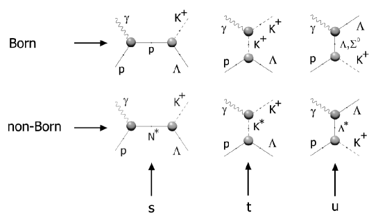
Figure 1: The tree-level contributions to the $p(\gamma,K^{+})\Lambda$ amplitude are shown. The Born terms with a ground-state hadron exchanges and the non-Born terms with nucleon-, kaon- and hyperon-resonance exchanges are shown in the upper and lower rows, respectively.

Since there exists no dominant resonance in photoproduction of kaons, unlike in $\pi$ or $\eta$ photoproduction, one has to take into account a priori more than 20 resonances with the mass $\leq 2\,\mbox{GeV}$ (see Tab. 1). This leads to a huge number of possible resonance configurations that should be investigated AS ; SL ; RPR11 , still resulting in a large number of models that describe the data quite well (with a small $\chi^{2}$). To reduce this large number of models one imposes constraints to acceptable values of the K$\Lambda$N and K$\Sigma$N coupling constants relating them to the well known $\pi$NN value by means of the SU(3) symmetry AS ; SL ; Jan01A .

One of the characteristic features of the $p(\gamma,K^{+})\Lambda$ process described by an isobar model is a too large contribution of the Born terms to the cross sections which largely overpredicts the data. To get a realistic description of the cross sections and the other observables allowing analysis of the resonant content of the amplitude, the nonphysically large strengths of the Born terms have to be reduced. This can be achieved by the introduction of form factors into the strong vertexes (hadron form factors) KM or by exchanges of several hyperon resonances SL or by a combination of both methods Jan01A ; Jan01B . In our model we combine both methods. Needless to say, the choice of the method strongly affects the dynamics of the model. Note that this problem is not present in the Regge-plus-resonance model GentRPR07 ; RPR11 .

Another ambiguity in construction of the gauge-invariant Lagrangian arises from a coupling in the K$\Lambda$N vertex which can be either pseudoscalar- or pseudovector-like PSPV . Whereas the former makes the total contribution of the Born terms gauge invariant the use of the latter requires introducing the contact term even with no form factors inserted. The role of these couplings was investigated in the threshold region Mart and it was concluded that both couplings can describe the K$\Lambda$ photoproduction data very well. In this work we have used the pseudoscalar coupling as in the most of isobar models.

To ensure a regularity of the tree-level invariant amplitude in the physical region the poles corresponding to the resonances are shifted into the complex plane, $m_{R}\to m_{R}-\texttt{i}\Gamma_{R}/2$, introducing the decay width $\Gamma_{R}$ which accounts for a finite lifetime of the resonant state. Then the Feynman propagator can be written as

$$\frac{1}{\not\!q-m_{R}+\texttt{i}\Gamma_{R}/2}=\frac{\not\!q+m_{R}-\texttt{i}\Gamma_{R}/2}{q^{2}-m^{2}_{R}+\texttt{i}m_{R}\Gamma_{R}+\Gamma_{R}^{2}/4}$$ (1)

and the following approximations are assumed in various isobar models

$$\frac{\not\!q+m_{R}}{q^{2}-m^{2}_{R}+\texttt{i}m_{R}\Gamma_{R}}$$ (2)

in the Saclay-Lyon and Gent models or

$$\frac{\not\!q+m_{R}-\texttt{i}\Gamma_{R}/2}{q^{2}-m^{2}_{R}+\texttt{i}m_{R}\Gamma_{R}}$$ (3)

in the Kaon-MAID model and in Ref. SF . In the tree-level approximation, the decay widths can mimic to some extent a dressing of the propagator. In most of the isobar models the widths are assumed as constant parameters, and the Breit-Wigner values suggested in the Particle Data Tables are used. In order to approximately account for unitarity corrections in the single-channel approach, the energy-dependent widths for the nucleon resonances were used in the KM model. The energy dependence of $\Gamma_{R}$ is given by a possibility of resonance decay into various opened channels. In this work we use the approximation (2) with constant decay widths.

	Nickname	Particle	Mass	Width	$J^{\pi}$	Status
			[MeV]	[MeV]
	${\rm K}^{*}$	$K^{*}(892)$	891.66	50.8	$1^{-}$
	K1	$K_{1}(1270)$	1272	90	$1^{+}$
	N1	$P_{11}(1440)$	1430	350	$1/2^{+}$	****
	N3	$S_{11}(1535)$	1535	150	$1/2^{-}$	****
	N4	$S_{11}(1650)$	1655	150	$1/2^{-}$	****
	N8	$D_{15}(1675)$	1675	150	$5/2^{-}$	****
	N9	$F_{15}(1680)$	1685	130	$5/2^{+}$	****
	N5	$D_{13}(1700)$	1700	150	$3/2^{-}$	***
	N6	$P_{11}(1710)$	1710	100	$1/2^{+}$	***
	N7	$P_{13}(1720)$	1720	270	$3/2^{+}$	****
	P5	$F_{15}(1860)$	1860	270	$5/2^{+}$	**
	P1	$P_{11}(1880)$	1870	235	$1/2^{+}$	**
	P4	$D_{13}(1875)$	1875	220	$3/2^{-}$	***
	P2	$P_{13}(1900)$	1900	500	$3/2^{+}$	***
	P3	$F_{15}(2000)$	2050	198	$5/2^{+}$	**
	L1	$\Lambda(1405)$	1405	50	$1/2^{-}$	****
	L2	$\Lambda(1600)$	1600	150	$1/2^{+}$	***
	L3	$\Lambda(1670)$	1670	35	$1/2^{-}$	****
	L4	$\Lambda(1800)$	1800	300	$1/2^{-}$	***
	L5	$\Lambda(1810)$	1810	150	$1/2^{+}$	***
	L6	$\Lambda(1520)$	1519.54	15.6	$3/2^{-}$	****
	L7	$\Lambda(1690)$	1690	60	$3/2^{-}$	****
	L8	$\Lambda(1890)$	1890	100	$3/2^{+}$	****
	S1	$\Sigma(1660)$	1660	100	$1/2^{+}$	***
	S2	$\Sigma(1750)$	1750	90	$1/2^{-}$	***
	S3	$\Sigma(1670)$	1670	60	$3/2^{-}$	****
	S4	$\Sigma(1940)$	1940	220	$3/2^{-}$	***

Table 1: Meson and baryon resonances which can be included in a description of the $p(\gamma,K^{+})\Lambda$ process. For each resonance, the mass, width, spin, parity, and status are shown. Entries are from Particle Data Tables 2014 PDG except for the P2 width which was taken from the Bayesian analysis of the Gent group.

II.1 Resonances with spin 3/2 and 5/2

The Rarita-Schwinger (R-S) description of high-spin fermion fields includes nonphysical degrees of freedom connected with their lower-spin content. If the R-S field is off its mass shell, the nonphysical parts may participate in the interaction, which is then called “inconsistent”. Almost two decades ago, Pascalutsa proposed a new consistent interaction theory for massive spin-3/2 fields Pasc , where the interaction is mediated by the spin-3/2 modes only. The consistency of the theory is ensured by the invariance of the spin-3/2 interaction vertexes under the local $U(1)$ gauge transformation of the R-S field. This scheme was generalized to arbitrary high spin by the Gent group Gent_spin and is used in this work.

The R-S propagator of the spin-3/2 field in terms of the spin-projection operators is Timm

$$S_{\mu\nu}(q)=\frac{\not\!q+m_{R}}{q^{2}-m_{R}^{2}+\texttt{i}m_{R}\Gamma_{R}}\,P_{\mu\nu}^{(3/2)}-\frac{2}{3m_{R}^{2}}(\not\!q+m_{R})\,P_{22,\mu\nu}^{(1/2)}+\frac{1}{m_{R}\sqrt{3}}\left(P_{12,\mu\nu}^{(1/2)}+P_{21,\mu\nu}^{(1/2)}\right),$$ (4)

where $P_{\mu\nu}^{(3/2)}$ projects on the spin-3/2 states

$$P_{\mu\nu}^{(3/2)}=g_{\mu\nu}-\frac{1}{3}\gamma_{\mu}\gamma_{\nu}-\frac{\not\!qq_{\nu}\gamma_{\mu}+q_{\mu}\gamma_{\nu}\not\!q}{3q^{2}},$$ (5)

and $P_{12,\mu\nu}^{(1/2)}$, $P_{21,\mu\nu}^{(1/2)}$, and $P_{22,\mu\nu}^{(1/2)}$ project on the spin-1/2 sector

$$P_{22,\mu\nu}^{(1/2)}=\frac{q_{\mu}q_{\nu}}{q^{2}},\,\,\,\,P_{12,\mu\nu}^{(1/2)}=\frac{q^{\rho}q_{\nu}\sigma_{\mu\rho}}{\sqrt{3}q^{2}},\,\,\,\,P_{21,\mu\nu}^{(1/2)}=\frac{q_{\mu}q^{\rho}\sigma_{\rho\nu}}{\sqrt{3}q^{2}},$$ (6)

where $\sigma_{\rho\nu}=\frac{\texttt{i}}{2}[\gamma_{\rho},\gamma_{\nu}]$.

The gauge invariance of the strong, $K(p_{K})\,\Lambda\,N^{*}(q)$, and electromagnetic, $N^{*}(q)\,p\,\gamma(k)$, couplings Pasc generates the transverse interaction vertexes

$$V^{S}_{\mu}(K\Lambda N^{*})=\frac{f}{m_{K}m_{R}}\,\epsilon_{\lambda\mu\alpha\beta}\,\gamma_{5}\,\gamma^{\alpha}\,q^{\lambda}\,p_{K}^{\beta}\,,$$ (7)

and

$$V^{EM}_{\nu}(N^{*}p\gamma)=\frac{\texttt{i}\,\gamma_{5}}{m_{R}(m_{R}+m_{p})}\,q^{\tau}\left[\;g_{1}F_{\tau\nu}+g_{2}\,(\,\gamma_{\tau}\gamma^{\sigma}F_{\nu\sigma}-\gamma_{\nu}\gamma^{\sigma}F_{\tau\sigma})\,\right]\,,$$ (8)

where $F_{\mu\nu}=k_{\mu}\varepsilon_{\nu}-\varepsilon_{\mu}k_{\nu}$, $\epsilon_{0123}=1$, and

$$V^{S}_{\mu}\,q^{\mu}\,=\,V^{EM}_{\nu}\,q^{\nu}\,=\,0\;.$$ (9)

Then it is obvious from Eqs. (4) and (6) that this property removes all non physical contributions of the spin-1/2 sector to the invariant amplitude. Moreover, one sees in Eq. (5) that the pole term in $P_{\mu\nu}^{(3/2)}$ also vanishes which makes it possible to include into the model the hyperon exchanges with the spin 3/2 in the u-channel (see Subsec. C below).

In general, for arbitrary high spin $n+1/2$ ($n$= 1, 2,..), the transversality of the interaction vertexes prevents the momentum-dependent terms in the propagator from contributing, allowing us to write the R-S propagator in the consistent theory only by means of the projection operator onto the pure spin-$(n+1/2)$ state Gent_spin :

$$S_{\mu_{1}\cdot\cdot\cdot\mu_{n},\nu_{1}\cdot\cdot\cdot\nu_{n}}(q)\to\frac{\not\!q+m_{R}}{q^{2}-m_{R}^{2}+\texttt{i}m_{R}\Gamma_{R}}{P}^{(n+1/2)}_{\mu_{1}\cdot\cdot\cdot\mu_{n},\nu_{1}\cdot\cdot\cdot\nu_{n}}(q).$$ (10)

The gauge invariance of the interaction results also in a relatively high-power momentum dependence in the invariant amplitude, which rises with rising spin of the R-S field as $\sim q^{2n}$ Gent_spin . For the spin-3/2 field it is apparent from Eqs. (7) and (8) that the momentum dependence is $\sim q^{\lambda}q^{\tau}$, see also (51) for the $s$-channel invariant amplitude. In the case of spin 5/2, the invariant amplitude can be schematically written as

$$\mathbb{M}_{NBs}^{N^{*}(5/2)}\sim q^{4}\frac{\not\!q+m_{R}}{q^{2}-m_{R}^{2}+\texttt{i}m_{R}\Gamma_{R}}{\cal P}^{(5/2)}_{\mu\nu,\lambda\rho}(q)\,{\cal O}^{\mu\nu,\lambda\rho}_{5/2},$$ (11)

where ${\cal P}^{(5/2)}_{\mu\nu,\lambda\rho}(q)$ projects onto the spin-5/2 state Gent_spin and ${\cal O}^{\mu\nu,\lambda\rho}_{5/2}$ stands for the remaining structure in the strong and electromagnetic vertexes, see (54).

This strong momentum dependence from derivatives in the gauge-invariant vertexes regularizes the amplitude, but it also causes nonphysical structures in the energy dependence of the cross section, which needs to be cut off especially above the resonance region. Therefore, the hadron form factors with a higher, spin-dependent energy power in the denominator and with relatively small values of the cut-off parameter in comparison with standard hadron form factors are used in the RPR model Gent_spin ; RPR11 . We have, therefore, also carefully investigated this property in our isobar approach considering various forms of the hadron form factor, see Subsec. D below.

Note that after the substitution $\sqrt{s}\to m_{R}$ the propagator used in the SL model SL equals that in Eq. (4). The interaction Lagrangians in SL, constructed as the most general form invariant under the so-called point transformation SLA , lead in general to an inconsistent description. Moreover, this point-transformation invariance adds three more free parameters, the off-shell parameters, to each spin-3/2 resonance SLA ; Jan01A ; Jan01B ; Jan02 . Using the consistent formalism in our approach we have avoided this additional uncertainty in the model.

II.2 Nucleon and kaon resonances

In selection of a set of baryon resonances that preferably describe the world’s $p(\gamma,K^{+})\Lambda$ data, one has to perform thousands of fits assuming all acceptable resonance combinations. To our knowledge, such a robust analysis has been performed by Adelseck and Saghai AS , further extended by the Saclay-Lyon group SL and by the Gent group RPR11 using more sophisticated technique in the data analysis based on a Bayesian inference method. Another data analysis in the multipole approach was performed by Mart and Sulaksono MartSu who considered resonances with the spin up to 9/2 with 93 free parameters performing the $\chi^{2}$ minimization fits to CLAS, SAPHIR, and LEPS data. The Gent group made the Bayesian test of a huge number of nucleon resonance combinations and selected two sets of the resonances with highest evidence values. We have chosen one of these solutions, RPR-2011A RPR11 , as the starting point in our analysis. The corresponding resonances are: N3, N4, N7, N9, P1, P2, P3, and P4 (see Tab. 1 for the notation). Since we limit ourselves only to the $K^{+}\Lambda$ channel, there is no need to introduce $\Delta$ resonances which cannot decay to $K^{+}\Lambda$ due to isospin conservation.

The four-star resonance N3 ($S_{11}(1535)$), which is of crucial importance for the description of $\eta$ photoproduction, lies below the K$\Lambda$ threshold, but its coupling to the K$\Lambda$ channel is possible due to its large width and predicted strong coupling to the strangeness sector. In the Bayesian analysis with the RPR model the N3 resonance was found to contribute with a moderate probability RPR11 whereas in the isobar model its coupling strength to the K$\Lambda$ channel was found to be quite small S1535 .

In the KM and Gent isobar models, the N4, N6, and N7 established resonances were chosen along with the missing resonances P4 ($D_{13}(1875)$) and P1 ($P_{11}(1880)$), respectively. In the SL model SL for the K$\Lambda$ electroproduction, only the well established resonances N1, N7, and N8 were selected. The older RPR model, RPR2007 GentRPR07 , selected N4, N6, N7, P2, and P4 resonances. The resonances N1, N6, and N8 were ruled out in the new Bayesian analysis whereas N4 and N7 and the missing P1, P2, and P4 resonances were confirmed. Note that due to large decay widths of most resonances their contributions overlap each other resulting in interference among many states. This makes the analysis of the resonance content of the invariant amplitude difficult, and even though high-quality data are available it still brings uncertain results (several possible solutions).

In the past, nucleon resonances P3 and P5 were considered as a one state only. Recently, the Particle Data Group PDG decided to consider them as two separate states. Since both of these states have only two-star status, they are not included in the PDG Summary Tables.

In many studies the vector K^∗ and pseudovector K₁ meson resonances were found to be important in the data description SL ; WJC and are used in all realistic isobar models. We have therefore included them in the basic resonance set. Let us remind that these two states together with the kaon are the lowest poles in the K⁺ and K^∗ Regge trajectories included in the Regge Guidal and RPR GentRPR07 ; RPR11 models, which also corroborates the importance of these states.

II.3 Hyperon resonances

The exchanges of hyperon resonances in the u-channel contribute to the background and were not included in some isobar models, e.g., in KM. They can play, however, an important role in the dynamics as shown in the SL SL and Gent isobar Jan01A ; Jan01B models. Particularly, they can compensate the nonphysically big contributions of the Born terms. Moreover, their presence can significantly improve description of data, reduce the $\chi^{2}$ and shift the value of the hadron cut-off parameter to a harder region MartY .

Formerly, mainly spin-1/2 hyperon resonances were included in the models with inconsistent description of the spin-3/2 baryons. To our knowledge, the only attempt to include a spin-3/2 hyperon resonance in the isobar model was done by the Saclay-Lyon group in Ref. SLA , the version “C” of the SL model. The reason for this limitation was that the pole in the $u=q^{2}$ variable, which appears in the invariant amplitude from the projection operator of the propagator (4), lies in the physical region ($u=0$) causing a divergence of the amplitude with the inconsistent interaction. In the consistent formalism, the pole term does not contribute owing to the transversality of the interaction vertexes, Eq. (9), and regularity of the amplitude,

$$V^{EM}_{\mu}(N^{*}p\,\gamma)\;\frac{\not\!q+m_{R}}{u-m_{R}^{2}+\texttt{i}m_{R}\Gamma_{R}}\,\frac{1}{3u}(\not\!q\,q^{\nu}\gamma^{\mu}+q^{\mu}\gamma^{\nu}\not\!q)\;V^{S}_{\nu}(K\Lambda N^{*})=0,$$ (12)

leaving only nonzero contributions from the momentum-independent terms in the projection operator (5). It is therefore safe to include the spin-3/2 hyperon resonances with relatively small masses, see Tab.I, which are expected to be important in describing the background.

Here we have considered only the spin-3/2 $\Lambda$ and $\Sigma$ well established four- or three-star resonances as reported in the Particle Data Tables 2014 PDG (Table I): $\Lambda(1520)\,3/2^{-}$ (L6), $\Lambda(1690)\,3/2^{-}$ (L7), and $\Lambda(1890)\,3/2^{+}$ (L8), with the branching ratios to $N\bar{K}$ 45%, 20-30%, and 20-35%, respectively; $\Sigma(1670)\,3/2^{-}$ (S3) and $\Sigma(1940)\,3/2^{-}$ (S4) with 7-13% and $<$20%, respectively.

II.4 Hadron form factors

Apart from reduction of the Born terms, the hadron form factor can also mimic the internal structure of hadrons in the strong vertexes, which is neglected in the hadrodynamical approach. However, there is still an ambiguity in the selection of a form of the hadron form factor: one can choose among dipole $F_{d}$, multidipole $F_{md}$, Gauss $F_{G}$, or multidipole Gauss shape $F_{mdG}$ Gent_spin :

$$F_{d}(x,m_{R},\Lambda_{R})= \,\frac{\Lambda_{R}^{4}}{(x-m_{R}^{2})^{2}+\Lambda_{R}^{4}},$$ (13a)

$$F_{md}(x,m_{R},\Lambda_{R},J_{R})= \,F_{d}^{J_{R}+1/2}(x,m_{R},\Lambda_{R}),$$ (13b)

$$F_{G}(x,m_{R},\Lambda_{R})= \,\exp[-(x-m_{R}^{2})^{2}/\Lambda_{R}^{4}],$$ (13c)

$$\begin{split}F_{mdG}(x,m_{R},\Lambda_{R},J_{R},\Gamma_{R})=&\,F_{d}^{J_{R}-1/2}(x,m_{R},m_{R}\tilde{\Gamma}_{R})\,F_{G}(x,m_{R},\Lambda_{R}),\end{split}$$ (13d)

where $m_{R}$, $J_{R}$, $\Lambda_{R}$, and $x\equiv s,t,u$ stands for the mass and spin of the particular resonance, cut-off parameter of the form factor, and Mandelstam variables, respectively. Moreover, it is required to introduce a modified decay width

$$\tilde{\Gamma}_{R}(J_{R})=\frac{\Gamma_{R}}{\sqrt{2^{1/2J_{R}}-1},}$$ (14)

which depends on the spin of the resonance and leads to preserving the interpretation of the resonance decay width as the full width in half maximum (FWHM) of the resonance peak Gent_spin .

Since the high-power momentum dependence of the amplitude leads to a substantial growth of the resonance contribution to the cross section, we need to introduce a hadron form factor to refine this behavior. In fact, the form factor should ensure that the resonant diagram does not contribute far from the mass pole of the exchanged particle. Unfortunately, with the form factor the cut-off dependence is introduced into the cross section. In Fig. 2, we demonstrate the dependence for the contribution of a particular resonance with spin 5/2 in the s-channel using the dipole (13a), multidipole (13b), Gauss (13c), and multidipole Gauss (13b) form factors with various values of the cut-off parameters. The use of the dipole form factor leads to enlarging the tail of the resonant peak whereas the Gauss form factor creates an artificial cut-off-value dependent peak while the actual resonant peak contributes only as its shoulder. Introducing the spin-dependent form factor, multidipole or multidipole Gauss, makes the effect moderate even for larger values of the cut-off parameter. Using the latter form factor makes the contribution almost independent of the cut-off value producing the real resonance pattern in the cross section (see Fig. 2).

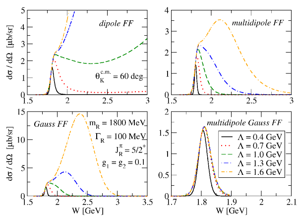
Figure 2: (Color online) Contribution of the spin-5/2 resonance with the mass 1800 and width 100 MeV to the cross section using different form factors. The cut-off dependence of the contribution is shown: the larger the cut-off value $\Lambda$, the more pronounced the effect.

The total amplitude constructed with the help of the effective Lagrangians is gauge invariant. The resonant amplitudes and the u-channel Born contribution are gauge-invariant on their own, the gauge non-invariant terms occur in the s- and t-channel Born contributions, see Eqs. (39) and (43) in Appendix A. However, these terms cancel in the sum of these two Born contributions. Unfortunately, while introducing the hadron form factors, these gauge noninvariant terms no longer cancel. The remedy is to introduce a contact term which ensures the gauge invariance Jan01A , see Appendix B for more details.

The generally accepted cut-off values lie in the range from approximately $0.7$ to $3.0\,\mbox{GeV}$; the lower the cut-off, the stronger the suppression. The values around the lower limit are considered too soft, and the form factors are, in this situation, regarded as a rather artificial tool to suppress the Born term contribution. As our analysis showed, obtaining a harder cut-off value is much easier than a softer one, which we attribute to the presence of many hyperon resonances in background.

Values of the cut-off parameters are established when optimizing the model parameters against experimental data. A single common cut-off value $\Lambda_{R}$ is assumed for all resonant diagrams whereas for the background terms another value $\Lambda_{bgr}$ is used.

III Observables

In the electroproduction

$${\rm e}(k_{1})+{\rm p}(p)\to{\rm e}(k_{2})+{\rm K^{+}}(p_{K})+\Lambda(p_{\Lambda}),$$

the transition amplitude in the one-photon exchange approximation is a product of the matrix elements of the hadron $\mathbb{J}^{\mu}$ and lepton $l_{\mu}=e\,\bar{u}(k_{2})\gamma_{\mu}u(k_{1})$ currents mediated by the photon propagator

$${M}_{fi}=\frac{1}{k^{2}}\,l_{\mu}\,\mathbb{J}^{\mu}(k^{2},s,t,u)\,,$$ (15)

where $k=k_{1}-k_{2}$ is the four-momentum of the virtual photon and $s=(p+k)^{2}$, $t=(p_{K}-k)^{2}$, and $u=(p_{\Lambda}-k)^{2}$ are the Mandelstam variables. Conservation of the hadron and lepton currents implies $\mathbb{J}^{\mu}k_{\mu}=l^{\mu}k_{\mu}=0$. The matrix element of the hadron current therefore can be decomposed into the linear combination of six covariant gauge-invariant contributions

$$\mathbb{J}^{\mu}\varepsilon_{\mu}=\sum_{j=1}^{6}\,\mathcal{A}_{j}(k^{2},s,t,u)\;\bar{u}(p_{\Lambda})\,\gamma_{5}\,\mathcal{M}_{j}\,u(p)\,,$$ (16)

where $\mathcal{M}_{j}$ are explicitly gauge-invariant operators

$$\mathcal{M}_{1} =(\not\!k\not\!\varepsilon-\not\!\varepsilon\not\!k)/2,$$ (17a)

$$\mathcal{M}_{2} =p\cdot\varepsilon-k\cdot p\,k\cdot\varepsilon/k^{2},$$ (17b)

$$\mathcal{M}_{3} =p_{\Lambda}\cdot\varepsilon-k\cdot p_{\Lambda}\,k\cdot\varepsilon/k^{2},$$ (17c)

$$\mathcal{M}_{4} =\not\!\varepsilon k\cdot p-\not\!kp\cdot\varepsilon,$$ (17d)

$$\mathcal{M}_{5} =\not\!\varepsilon k\cdot p_{\Lambda}-\not\!kp_{\Lambda}\cdot\varepsilon,$$ (17e)

$$\mathcal{M}_{6} =\not\!kk\cdot\varepsilon-\not\!\varepsilon k^{2},$$ (17f)

and $\varepsilon_{\mu}$ is the polarization vector of the virtual photon. The scalar amplitudes $\mathcal{A}_{j}(k^{2},s,t,u)$ contain contributions from the considered tree-level Feynman diagrams. Their expressions for various types of particle exchanges are given in Appendix A. In the photoproduction case ($k^{2}=0$), there are only four terms in the decomposition (16) AS .

In the calculations which involve also a non relativistic input, e.g., the calculation of the hypernucleus production cross sections HProd with non relativistic wave functions of the nucleus and hypernucleus, one also needs a more convenient representation of the Lorentz invariant matrix element (16) in terms of the two-component spinor amplitudes known as the Chew, Goldberger, Low, and Nambu (CGLN) amplitudes AS ; SL ; SF . These amplitudes are, however, also widely used in calculations of observables in the elementary process. In the c.m. frame, the Lorentz invariant matrix element (16) can be written as

$$\mathbb{J}^{\mu}\varepsilon_{\mu}=\chi_{\Lambda}^{+}\,{\cal F}\,\chi_{\rm p}$$ (18)

where $\chi_{\rm p}$ and $\chi_{\Lambda}$ are the Pauli spinors and

$${\cal F}=f_{1}\,\vec{\sigma}\cdot\vec{\varepsilon}-\texttt{i}f_{2}\,\vec{\sigma}\cdot\hat{\vec{p}}_{K}\,\vec{\sigma}\cdot(\hat{\vec{k}}\times\vec{\varepsilon})+f_{3}\,\vec{\sigma}\cdot\hat{\vec{k}}\,\hat{\vec{p}}_{K}\cdot\vec{\varepsilon}+f_{4}\,\vec{\sigma}\cdot\hat{\vec{p}}_{K}\,\hat{\vec{p}}_{K}\cdot\vec{\varepsilon}+f_{5}\,\vec{\sigma}\cdot\hat{\vec{k}}\,\hat{\vec{k}}\cdot\vec{\varepsilon}+f_{6}\,\vec{\sigma}\cdot\hat{\vec{p}}_{K}\,\hat{\vec{k}}\cdot\vec{\varepsilon}.$$ (19)

Here $\hat{\vec{k}}=\vec{k}/|\vec{k}|$, $\hat{\vec{p}}_{K}=\vec{p}_{K}/|\vec{p}_{K}|$, $\vec{\sigma}$ are the Pauli matrices, and $\vec{\varepsilon}$ is the spatial component of the virtual-photon polarization vector. The CGLN amplitudes $f_{i}(k^{2},s,t,u)$ are expressed via the scalar amplitudes $A_{j}$

$$f_{1} =N^{*}[-(W-m_{p})\mathcal{A}_{1}+k\cdot p\,\mathcal{A}_{4}+k\cdot p_{\Lambda}\,\mathcal{A}_{5}-k^{2}\mathcal{A}_{6}],$$ (20a)

$$f_{2} =N^{*}\frac{|\vec{k}||\vec{p}_{K}|}{(E^{*}_{\Lambda}+m_{\Lambda})(E_{p}^{*}+m_{p})}[(W+m_{p})\mathcal{A}_{1}+k\cdot p\,\mathcal{A}_{4}+k\cdot p_{\Lambda}\,\mathcal{A}_{5}-k^{2}\mathcal{A}_{6}],$$ (20b)

$$f_{3} =-N^{*}\frac{|\vec{k}||\vec{p}_{K}|}{E_{p}^{*}+m_{p}}[\mathcal{A}_{3}+(W+m_{p})\mathcal{A}_{5}],$$ (20c)

$$f_{4} =N^{*}\frac{|\vec{p}_{K}|^{2}}{E_{\Lambda}^{*}+m_{\Lambda}}[\mathcal{A}_{3}-(W-m_{p})\mathcal{A}_{5}],$$ (20d)

$$f_{5} =N^{*}\frac{|\vec{k}|^{2}}{E_{p}^{*}+m_{p}}\bigg{[}\mathcal{A}_{1}-\frac{1}{k^{2}}[(k^{2}+k\cdot p)\mathcal{A}_{2}+k\cdot p_{\Lambda}\,\mathcal{A}_{3}]-(W+m_{p})(\mathcal{A}_{4}+\mathcal{A}_{6})\bigg{]},$$ (20e)

$$\begin{split}f_{6}&=N^{*}\frac{E_{\gamma}^{*}|\vec{k}||p_{K}|}{(E^{*}_{\Lambda}+m_{\Lambda})(E^{*}_{p}+m_{p})}\bigg{\{}\mathcal{A}_{1}-m_{p}\mathcal{A}_{4}+\frac{k\cdot p_{\Lambda}}{E_{\gamma}^{*}}\mathcal{A}_{5}+\frac{(E^{*}_{p}+m_{p})}{E_{\gamma}^{*}k^{2}}[(k^{2}+k\cdot p)\mathcal{A}_{2}\\ &\;\;\;\;+k\cdot p_{\Lambda}\,\mathcal{A}_{3}]-(W+m_{p})\mathcal{A}_{6}\bigg{\}},\end{split}$$ (20f)

where $W=\sqrt{s}$ and $E_{p}^{*}$, $E_{\Lambda}^{*}$, $E_{K}^{*}$, and $E_{\gamma}^{*}$ are the c.m. energies of the proton, hyperon, kaon, and photon, respectively. The normalization factor reads

$$N^{*}=\sqrt{\frac{(E^{*}_{\Lambda}+m_{\Lambda})(E^{*}_{p}+m_{p})}{4m_{\Lambda}m_{p}}}.$$ (21)

The triple-differential cross section for electroproduction of unpolarized hyperon with unpolarized electron beam and target is obtained as

$$\frac{\mbox{d}^{3}\sigma}{\mbox{d}E_{e^{\prime}}\mbox{d}\Omega_{e^{\prime}}\mbox{d}\Omega_{K}^{c.m.}}=\Gamma\bigg{[}\sigma_{T}+\varepsilon\sigma_{L}+\varepsilon\sigma_{TT}\cos 2\phi_{K}+\sqrt{2\varepsilon_{L}(\varepsilon+1)}\sigma_{LT}\cos\phi_{K}\bigg{]},$$ (22)

where $\phi_{K}$, $\Gamma$, $\varepsilon$, and $\varepsilon_{L}$ are the angle between the lepton and hadron planes, the virtual-photon flux factor, and the transverse and longitudinal photon polarization parameters, respectively SF . The response functions $\sigma_{T}$ and $\sigma_{L}$ describe the cross sections for the unpolarized and longitudinally polarized photon beams, respectively, while $\sigma_{TT}$ stands for the asymmetry of a transversally polarized photon beam. The last term containing $\sigma_{LT}$ describes the interference effects between the longitudinal and transverse components of the photon beam. Note that $\sigma_{T}$ and $\sigma_{TT}$ correspond to the cross section and beam asymmetry in the photoproduction process, respectively. The response functions in terms of the CGLN amplitudes read as follows

$$\sigma_{T}= \,C\,\texttt{Re}\bigg{\{}|f_{1}|^{2}+|f_{2}|^{2}-2f_{1}f_{2}^{*}\cos\theta_{K}+\sin^{2}\theta_{K}\bigg{[}\frac{1}{2}(|f_{3}|^{2}+|f_{4}|^{2})+f_{1}f_{4}^{*}+f_{2}f_{3}^{*}+f_{3}f_{4}^{*}\cos\theta_{K}\bigg{]}\bigg{\}},$$ (23a)

$$\sigma_{L}= \,C\,\texttt{Re}\left\{|\tilde{f}_{5}|^{2}+|\tilde{f}_{6}|^{2}+2\tilde{f}_{5}\tilde{f}_{6}^{*}\cos\theta_{K}\right\},$$ (23b)

$$\sigma_{TT}= \,C\,\texttt{Re}\bigg{\{}\frac{1}{2}(|f_{3}|^{2}+|f_{4}|^{2})+f_{1}f_{4}^{*}+f_{2}f_{3}^{*}+f_{4}f_{3}^{*}\cos\theta_{K}\bigg{\}}\sin^{2}\theta_{K},$$ (23c)

$$\sigma_{LT}= -C\,\texttt{Re}\bigg{\{}(f_{1}+f_{4})\tilde{f}_{6}^{*}+(f_{2}+f_{3})\tilde{f}_{5}^{*}+(f_{3}\tilde{f}_{6}^{*}+f_{4}\tilde{f}_{5}^{*})\cos\theta_{K}\bigg{\}}\sin\theta_{K},$$ (23d)

where we have defined the linear combinations

$$\tilde{f}_{5}= f_{1}+f_{3}\cos\theta_{K}+f_{5},$$ (24)

$$\tilde{f}_{6}= f_{4}\cos\theta_{K}+f_{6}$$ (25)

and the normalization factor $C$ is given as

$$C=(\hbar c)^{2}\frac{\alpha}{4\pi}\frac{m_{\Lambda}|\vec{p}_{K}|}{|\vec{k}|W}.$$ (26)

The general expression for the electroproduction cross section considering all three possible types of polarization can be found in Ref. Koch . Here we give only the single-polarization observables in photoproduction which we use in the analysis and which in terms of the CGLN amplitudes read

$$P =-\texttt{Im}[2f_{1}^{*}f_{2}+f_{1}^{*}f_{3}-f_{2}^{*}f_{4}-(f_{2}^{*}f_{3}-f_{1}^{*}f_{4})\cos\theta_{K}-f_{3}^{*}f_{4}\sin^{2}\theta_{K}]\sin\theta_{K},$$ (27)

$$\Sigma =-\texttt{Re}[(|f_{3}|^{2}+|f_{4}|^{2})/2+f_{2}^{*}f_{3}+f_{1}^{*}f_{4}+f_{3}^{*}f_{4}\cos\theta_{K}]\sin^{2}\theta_{K},$$ (28)

$$T =\texttt{Im}[f_{1}^{*}f_{3}-f_{2}^{*}f_{4}+\cos\theta_{K}(f_{1}^{*}f_{4}-f_{2}^{*}f_{3})-f_{3}^{*}f_{4}\sin^{2}\theta_{K}]\sin\theta_{K},$$ (29)

where $P$, $\Sigma$ and $T$ stands for hyperon polarization, beam asymmetry (see also Eq. (23c)) and target polarization, respectively.

IV Fitting model parameters

Since the isobar model is an effective model with the coupling constants and cut-off values of hadron form factors undetermined, our goal is to fixate these free parameters to the experimental data during the fitting process.

The free parameters to be adjusted are the coupling constants of the Born terms $g_{K\Lambda N}$ and $g_{K\Sigma N}$, the nucleon, kaon and hyperon resonances and two cut-off parameters of the hadron form factor. Each spin-1/2 resonance contributes with one parameter whereas higher-spin resonances as well as kaon resonances contribute with two parameters. As well as in the well-known Kaon-MAID model, we assume a single cut-off value $\Lambda_{R}$ for all resonant (s-channel) diagrams whereas for background terms another value $\Lambda_{bgr}$ is used. Altogether, the number of free parameters varies from 20 to 25 depending on the number and spin of considered nucleon and hyperon resonances.

In order to test whether a given hypothetical function describes the given data well, the $\chi^{2}$ is calculated. The optimum set of free parameters $(c_{1},\ldots,c_{n})$ for a given set of data points $(d_{1},\ldots,d_{N})$ is that with the lowest value of $\chi^{2}$. The $\chi^{2}$ is

$$\chi^{2}=\sum_{i=1}^{N}\frac{[d_{i}-p_{i}(c_{1},\ldots,c_{n})]^{2}}{(\sigma_{d_{i}}^{tot})^{2}},$$ (30)

where $N$ is the number of data points and $n$ the number of free parameters; $p_{i}$ represents the theoretical prediction of observables (differential cross section, hyperon polarization and beam asymmetry in our case) for the measured data point $d_{i}$, with the total error given as

$$\sigma_{d_{i}}^{tot}=\sqrt{(\sigma_{d_{i}}^{sys})^{2}+(\sigma_{d_{i}}^{stat})^{2}},$$ (31)

where $\sigma_{d_{i}}^{sys}$ and $\sigma_{d_{i}}^{stat}$ represent systematic and statistical errors of a given datum, respectively. Whereas systematic errors tend to be strongly correlated within a given data set, the correlation weakens when using several independent subsets. Since we assume several data sets (see subsection IV.1), we have adopted the definition (31) similarly to the analysis by Adelseck and Saghai AS . Some groups, e.g., the Gent group, use an even more conservative prescription for the total error RPR11 .

In order to obtain the optimum set of parameters, one is forced to minimize $\chi^{2}$ in the $n$ dimensional space. In the ideal case, $\chi^{2}=\text{n.d.f.}$, where $\text{n.d.f.}=N-n$ is the number of degrees of freedom.

The minimization was performed with the help of the least-squares fitting procedure using the MINUIT code CERN . Since MINUIT uses a nonlinear transformation for the parameters with limits, which makes the accuracy of the resulting parameter worse when it approaches a boundary value, the limits should be avoided if they are not necessary to prevent the parameter from reaching nonphysical values. The main coupling constants $g_{K\Lambda N}$ and $g_{K\Sigma N}$ were kept inside the limits of 20% broken SU(3) symmetry

$$-4.4\leq \,\frac{g_{K\Lambda N}}{\sqrt{4\pi}}\leq-3.0,$$ (32a)

$$0.8\leq \,\frac{g_{K\Sigma N}}{\sqrt{4\pi}}\leq 1.3.$$ (32b)

In order to avoid too soft or too hard form factors, the cut-off parameters of the hadron form factor were kept inside the limits from $0.7$ to $3.0\,\mbox{GeV}$.

The coupling parameters entering the fitting procedure are always products of the strong and electromagnetic coupling constants. In order to guarantee a correct dimension of the interacting Lagrangians, the coupling constants have to be normalized appropriately. Since the Lagrangian for the spin-3/2 nucleon resonance contains two derivatives of the R-S field, the coupling parameters read

$$G_{1}= \frac{fg_{1}}{m_{R}^{2}m_{K}(m_{R}+m_{p})},$$ (33a)

$$G_{2}= \frac{fg_{2}}{m_{R}^{2}m_{K}(m_{R}+m_{p})}.$$ (33b)

In the case of spin-3/2 hyperon resonances, $m_{p}$ is replaced with $m_{\Lambda}$. Analogously, the spin-5/2 coupling parameters are normalized as follows

$$G_{1}= -\frac{fg_{1}}{16m_{K}^{4}m_{p}^{4}},$$ (34a)

$$G_{2}= -\frac{fg_{2}}{32m_{K}^{4}m_{p}^{5}}.$$ (34b)

The high mass powers in the denominator result in very small values of $G_{i}$ for $N^{*}(5/2)$ in comparison with the coupling parameters of lower-spin nucleon resonances.

The hyperon coupling parameters tend to be very large compared with coupling parameters of other resonances. Therefore, we did not take into account results with hyperon coupling parameters significantly bigger than 10.

IV.1 Experimental data

Recently, new precise data from LEPS, GRAAL and particularly from CLAS collaborations became available. For the fitting procedure, we selected around 3400 data points stemming from CLAS and LEPS collaborations with addition of several tens of data points collected by Adelseck and Saghai AS . Namely, we used the CLAS 2005 CLAS05 , CLAS 2010 CLAS10 , and LEPS LEPS cross-section data, CLAS 2010 hyperon polarization data CLAS10 , and LEPS beam asymmetry data LEPS .

In our analysis, we are concerned mainly with the resonance region and therefore have restricted the CLAS 2010 data sets to the energy range up to $2.355\,\mbox{GeV}$ and $2.225\,\mbox{GeV}$ for the cross-section and hyperon polarization data, respectively.

Since the CLAS and SAPHIR SAPHIR data are not consistent with each other, especially in the forward-angle region ByMa which is of particular interest here, we decided not to use the SAPHIR cross-section data in the analysis. Unfortunately, the CLAS 2005 and CLAS 2010 data sets show inconsistency with each other of about one or two standard deviations in the threshold region for kaon angle less than approximately $60^{\circ}$.

IV.2 Results of fitting

While minimizing the $\chi^{2}$ it is important to find a global minimum. Since this task occurs in a huge parameter space that has a lot of local minima, the result of the fitting procedure often depends on starting values of the fitted parameters.

Generally, choosing the best solution is not an easy task. The $\chi^{2}$ value is only a mathematical tool showing the goodness of a fit. However, results with similar $\chi^{2}$ values can still give rather different predictions of the observables in some kinematic regions. Therefore, not only thorough inspection of the numerical values of the fitted parameters, but also a brief check of the predicted observables is welcome.

We have done several hundreds of fits considering various resonance configurations and different shapes of hadron form factor. While the set of nucleon resonances chosen in the RPR-2011A model provided us the starting point, we have considered many other resonant states during the procedure of fitting.

Since one cannot be sure that the detected minimum is the global one, we have selected several models with similar $\chi^{2}$. The models differ mainly in the choice of nucleon and hyperon resonances and their coupling constants, cut-off values of the hadron form factor, and the shape of the form factor. Particularly, the smallness of hyperon coupling constants plays an important role when deciding if the model should be rejected or not. Since the isobar model is only a tree-level approximation, the couplings even larger than 1 are still justifiable.

During the fitting procedure, we also tried to slightly modify the mass and width of several intermediate particles in the ranges provided by the Particle Data Tables 2014 PDG (or when there were no preferred values). On the one hand, this forced the models to improve their description of the cross section; especially the reduction of the width of P2 from $500\,\mbox{MeV}$ to a value of about $400\,\mbox{MeV}$ or less led to filling up the second peak in the cross-section data. On the other hand, the modification of the width of P2 resulted in a growth of the $\chi^{2}$ value and made the description of single-polarization observables worse.

In order to gain insight into the effect of high-spin resonances on the observables, some of the fits were performed with the inconsistent formalism for the spin-3/2 and spin-5/2 resonances used in the SL model. Particularly, the fit of the BS2 model (see below) with the inconsistent formalism led to an enlargement of the $\chi^{2}$ from $1.64$ to $1.91$, growth of the cut-off parameter for the hadron form factor to almost $3\,\mbox{GeV}$, and decrease of the cross-section prediction in the forward-angle region. In this fit we omitted the spin-3/2 hyperon resonance S4. Generally, the use of the inconsistent high-spin formalism results in larger couplings for spin-5/2 resonances which is due to a different normalization introduced into the coupling parameters (see Eq. (34)).

The main asset of the presence of high-spin hyperon resonances is the reduction of coupling parameters of spin-1/2 hyperon resonances. With no $Y^{*}(3/2)$ introduced, the couplings of $Y^{*}(1/2)$ tend to acquire values of the order of 10 or even more. While the $Y^{*}(3/2)$ are implemented, the couplings of both $Y^{*}(1/2)$ and $Y^{*}(3/2)$ are only exceptionally bigger than 10.

In the analysis, we examined the effect of distinct shapes of the hadron form factor on the resonance behavior. As seen from the definition (13), the multidipole form factor affects the resonance behavior more strongly than the dipole one. Therefore, introducing the multidipole form factor leads to bigger cut-off parameters for resonances ($\Lambda_{res}\sim 3\,\mbox{GeV}$) than considering the dipole form factor ($\Lambda_{res}\sim 2\,\mbox{GeV}$). Unfortunately, we were not able to achieve a single result with $\chi^{2}<2$ using the multidipole Gauss form factor. This shape of form factor was introduced by the Gent group in their Regge-plus-resonance model to strongly suppress the contribution of the nucleon resonances in the high-energy region. However, it seems there is no need to introduce such a strong form factor in the isobar model.

The predictions of the models with $\chi^{2}<2$ were tested in the comparison with the experimental data. Particularly, the comparison with hyperon polarization data can reveal a subtle interplay among many resonances. Even though the smallness of $\chi^{2}$ denotes a good agreement of the model prediction with the data, in the kinematic regions where data are scarce (e.g., the forward-angle region) the model predictions can still differ.

The best solutions regarding the smallness of the $\chi^{2}$, values of fitted parameters and correspondence with data were coined BS1 and BS2. Whereas the model coined BS1 was obtained using a multidipole form factor, the BS2 model was gained using a dipole shape of the form factor. Moreover, the mass of the P5 resonance was slightly modified from $1820\,\mbox{MeV}$ in the BS1 model to $1860\,\mbox{MeV}$ in the BS2 model.

	BS1	BS2	KM	SL
$g_{K\Lambda N}$	$-3.00$	$-3.00$	$-3.80$	$-3.16$
$g_{K\Sigma^{0}N}$	$1.11$	$0.80$	$1.20$	$0.91$
$G_{V}(K^{*})$	$-0.18$	$-0.17$	$-0.79$	$-0.05$
$G_{T}(K^{*})$	$0.02$	$-0.03$	$-2.63$	$0.16$
$G_{V}(K_{1})$	$0.28$	$0.30$	$3.81$	$-0.19$
$G_{T}(K_{1})$	$-0.28$	$-0.23$	$-2.41$	$-0.35$
$G(N1)$	–	–	–	$-0.02$
$G(N3)$	$0.10$	$0.17$	–	–
$G(N4)$	$-0.07$	$-0.05$	$-0.13$	–
$G(N6)$	–	$-0.05$	$-0.26$	–
$G_{1}(N7)$	$-0.09$	$-0.07$	$0.05$	$-0.04$
$G_{2}(N7)$	$-0.01$	$-0.0057$	$0.61$	$-0.14$
$G_{1}(N8)$	–	–	–	$-0.63$
$G_{2}(N8)$	–	–	–	$-0.05$
$G_{1}(P4)$	$0.21$	$0.23$	$1.10$	–
$G_{2}(P4)$	$0.26$	$0.26$	$0.63$	–
$G_{1}(P5)$	$-0.04$	$-0.02$	–	–
$G_{2}(P5)$	$0.04$	$0.02$	–	–
$G_{1}(P2)$	$0.11$	$0.09$	–	–
$G_{2}(P2)$	$-0.02$	$-0.01$	–	–
$G_{1}(P3)$	$-0.0003$	$-0.0018$	–	–
$G_{2}(P3)$	$-0.0029$	$-0.0015$	–	–
$G_{1}(N9)$	$0.05$	$0.03$	–	$-0.63$
$G_{2}(N9)$	$-0.05$	$-0.03$	–	$-0.05$
$G(L1)$	–	$9.67$	–	$-0.42$
$G(L3)$	–	–	–	$1.75$
$G(L4)$	$-8.39$	$-11.55$	–	–
$G(L5)$	–	–	–	$-1.96$
$G_{1}(L6)$	$0.86$	–	–	–
$G_{2}(L6)$	$-0.09$	–	–	–
$G_{1}(L8)$	$-2.33$	–	–	–
$G_{2}(L8)$	$0.0033$	–	–	–
$G(S1)$	$-11.58$	$-8.09$	–	$-7.33$
$G(S2)$	$15.77$	–	–	–
$G_{1}(S4)$	$-8.32$	$-0.86$	–	–
$G_{2}(S4)$	$0.81$	$0.18$	–	–
$\Lambda_{bgr}$	$1.88$	$1.94$	$0.64$	–
$\Lambda_{res}$	$2.74$	$2.15$	$1.04$	–
$\chi^{2}/\text{n.d.f.}$	$1.64$	$1.64$	–	–

Table 2: Coupling constants, cut-off values, and $\chi^{2}$ of the final models BS1 and BS2 are compared with the parameters of the Kaon-MAID and Saclay-Lyon models.

V Discussion of results

In this section we present the new isobar models BS1 and BS2 for photoproduction of K${}^{+}\Lambda$ and compare their predictions for the cross section, hyperon polarization, and beam asymmetry with the data and results of the older models Saclay-Lyon and Kaon-MAID. Note that the numerical results of the SL and KM models have been obtained by using our code with the parameters presented in Table 2.

The nucleon-resonance content of the BS1 and BS2 models almost does not differ, see Table 2. The BS2 contains only one more resonance N6 with a small coupling constant. The coupling constants of the other nucleon resonances have the same sign and their values are very similar. This set of $N^{*}$ significantly overlaps with that suggested by the Gent group. The only difference, except for N6, is that the two-star resonance P1 with spin 1/2 in the RPR was replaced with the almost equal mass two-star spin-5/2 resonance P5 in our models.

More differences between BS1 and BS2 are observed in description of the background. The values of the main coupling constants, $g_{K\Lambda N}$ and $g_{K\Sigma N}$, and those for $K^{*}$ and $K_{1}$ exchanges are very similar and the signs are identical except for the tensor coupling of $K^{*}$ which has the opposite sign. In both models the value of $g_{K\Lambda N}$ is at the upper limit allowed in fitting (32a), which suggests a considerable violation of SU(3) symmetry. Note that the differences in these coupling constants, particularly $g_{K\Sigma N}$ and $G_{T}(K^{*})$, might have an impact on the model predictions in the $n(\gamma,K^{0})\Lambda$ process HYP10 .

Significant differences are found in the included sets of the hyperon resonances and their couplings. The BS2 contains only one spin-3/2 hyperon resonance S4 and three spin-1/2 resonances L1, L4, and S1, whereas BS1 includes three spin-3/2 resonances L6, L8, and S4 and only one spin-1/2 resonance L4. The general feature of the presented models and other solutions found during the fitting procedure is that the coupling strengths of the hyperon exchanges tend to be relatively large in comparison with the typical values obtained for the couplings of the nucleon resonances. This experience is similar to that gained in the analyses by the Saclay-Lyon SL and Gent Jan01B groups on a role of the hyperon resonances in $p(\gamma,K^{+})\Lambda$. Note that in version C of the Saclay-Lyon model SLA the only $\Lambda(1890)\,$3/2⁺ (L8) resonance was included; they concluded, however, that this resonance is not required by the data set available at that time, i.e. before 1998. Reasonable values of the hyperon couplings, $-20\leq G(Y^{*})\leq 20$, were therefore used in our analysis as a criterion for a model selection. These observations suggest that, whereas the current new experimental data are able to fix relatively well the set of the nucleon resonances producing genuine resonance patterns in the observables, they still cannot determine uniquely the non-resonant part of the amplitude (background). Therefore, one still cannot select a set of hyperon resonances, contributing to the process, with certainty.

Let us note that, in view of the achieved quality of data description, the total number of resonances included in BS1 and BS2, 16 and 15, respectively, is quite moderate in comparison with the older models KM and SL and the recent models by Mart MartSu ; Mart and Maxwell Maxwell .

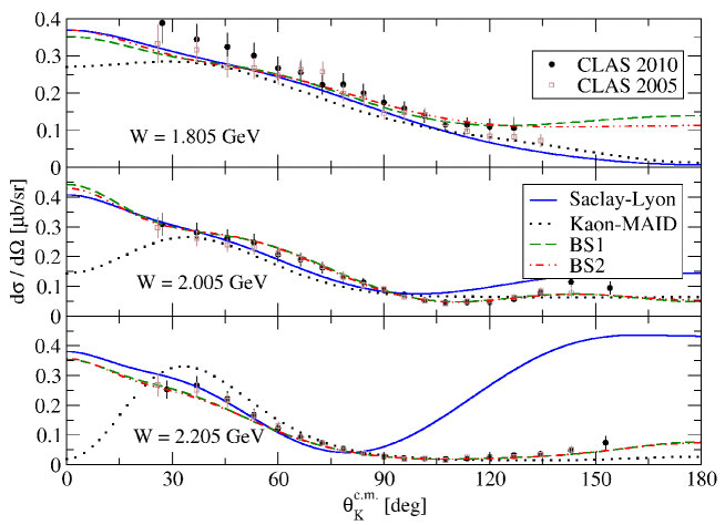
Figure 3: (Color online) Angular dependence of the cross sections is shown for three values of the c.m. energy. In the forward-angle region, the Saclay-Lyon (solid curve), BS1 (dashed curve), and BS2 (dash-dotted curve) models predict decreasing dependence of the cross section. In contrast the Kaon-MAID model (dotted curve) predicts a bump around $\theta_{K}^{c.m.}=30^{\circ}$. The data are from the CLAS 2005 CLAS05 and CLAS 2010 CLAS10 collaborations.

Angular dependence of the calculated cross sections in comparison with the CLAS data is shown in Fig. 3 for three energies. Both BS1 and BS2 models give very similar predictions which differ from predictions of the other models mainly in the forward- and backward-angle regions. In the small kaon-angle region, $\theta_{K}^{c.m.}<40^{\circ}$, the new models predict descending angular dependence like the SL model, contrary to the KM which predicts a very suppressed cross sections for energies $W\geq 2$ GeV. In the backward-angle region the models agree with the KM describing the data very well. The subtle difference between BS1 and BS2 model in the description of backward angles (apparent for $W=1.805\,\mbox{GeV}$) can be assigned to the sign change of the tensor coupling of $K^{*}$. One may conclude that the BS1 and BS2 models describe the cross sections in the full angular and considered energy regions very well. Note that the consistency of the cross sections in the very small kaon-angle region with the results of the SL model (Fig. 3) and the fact that these cross sections are dominated by the spin-flip part of the amplitude could predetermine the new models for successful predictions of the cross sections in the production of the hypernuclei, like the Saclay-Lyon model HProd ; JLab .

The model dynamics in the small-angle area is driven mainly by the background contributions in which the spin-1/2 hyperon resonances, surprisingly, play a very important role. In spite of their large contribution in the backward angles, they give the largest contribution in the forward-angle region when combined with the Born terms. On the other hand, the spin-3/2 hyperon resonances combined with the Born terms contribute predominantly in the backward-angle region. The role of the kaon resonances is to suppress the Born term contributions in the central-angle region.

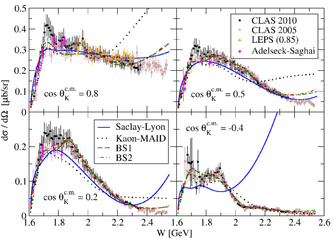
Figure 4: (Color online) Differential cross section in dependence on the c.m. energy $W$ is shown for various kaon angles. Notation of the curves is the same as in the Fig. 3. The data are from CLAS 2005 CLAS05 , CLAS 2010 CLAS10 , LEPS LEPS and from the publication of Adelseck and Saghai AS . The LEPS data are for $\cos\theta_{K}^{c.m.}=0.85$.

In Fig. 4 we show resonance effects in the energy dependent differential cross sections for four kaon angles as they are revealed by the data and the models. First, let us note that the resonance pattern revealed by the CLAS data around $W=1.7$ GeV for the forward angles is sharper in the CLAS data set from 2010 than in the older one from 2005. The new models predict conservative cross sections lying in between these data sets preferring rather the older data. The N6 in BS2 is not strong enough to make the peak around 1.7 GeV sharper. The older CLAS data set is also favored by the hybrid RPR-2011A and RPR-2011B models RPR11 . Both new isobar models BS1 and BS2 predict a peak around 1.9 GeV in the central- and backward-angle regions but not at very small angles. In the forward-angle region some strength is also apparent around $W=2$ GeV modeled by the higher-mass resonances P2, P3, and P4. The strong grow of the cross section in the threshold region is described by the BS1 and BS2 models satisfactorily, better than by the SL model.

The new isobar models, eligible for the resonance region, describe data well up to energy $W\approx 2.4$ GeV. Above this energy the cross sections systematically rise overshooting the data, which is more apparent at forward angles in Fig. 4 and which is a well-known feature of isobar models. In the new models, the contributions of the nucleon resonances in the s channel are regularized by the strong-enough hadron form factors as shown in Fig. 2. The high-energy divergence is therefore created mainly by the background part of the amplitude. This divergent behavior, however, differs for various models: in the KM model, predictions start diverging at forward angles above 2.2 GeV (the maximum energy for which the model was constructed) but predictions of the SL model strongly overshoot the data at backward angles above 2 GeV. This divergent behavior of the isobar models is also well seen in the energy dependence of the total cross section as shown in Fig. 5. Whereas the KM model begins to diverge at $E_{\gamma}^{lab}=2.2\,\mbox{GeV}$, i.e., beyond its scope, the SL model produces a divergent behaviour above $E_{\gamma}^{lab}=1.6\,\mbox{GeV}$. Note, however, that the KM, SL, and Gent models were fitted to the old SAPHIR data and, therefore, slightly underestimate the current CLAS data (see Fig. 20 in Ref. CLAS05 ).

The spin-3/2 and spin-5/2 nucleon resonances contributing mainly in the central-angle region are also important in the forward-angle region. They contribute in combination with the background terms. Moreover, they give rather diverse results: the spin-3/2 resonances raise the cross section making the peak around $\theta_{K}^{c.m.}=45^{\circ}$ whereas the spin-5/2 resonances lead to a decrease of the cross section for kaon angles around $60^{\circ}$.

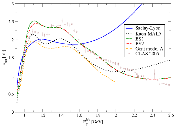
Figure 5: (Color online) Model predictions of the $p(\gamma,K^{+})\Lambda$ total cross section. For comparison, the Gent isobar model (model A) was added as read from Fig. 7 in Ref. Jan01A . Notation of the rest of the curves is the same as in the Fig. 3. Data stem from Fig. 20 in Ref. CLAS05 .

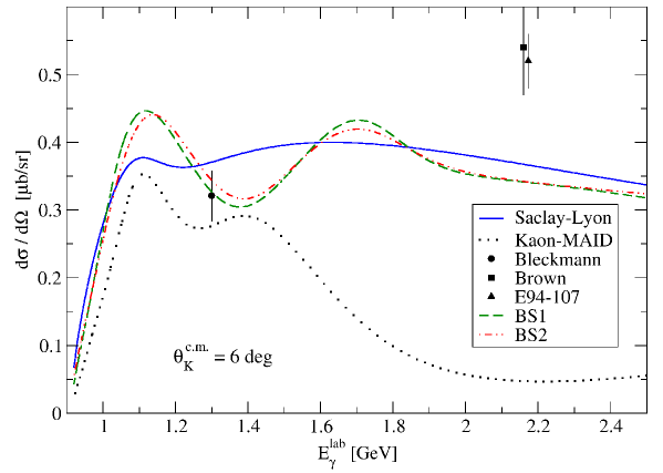
Figure 6: (Color online) Predictions of the differential cross section for photoproduction at $\theta_{K}^{c.m.}=6^{\circ}$ is shown for several models. The only available photoproduction data point in this region is from Bleckmann et al Bleck . The data points of Brown Brown and E94-107 E94-107 are for electroproduction with a very small value of the virtual-photon mass $|k^{2}|$. Notation of the curves is the same as in the Fig. 3.

In the extreme forward-angle region, the discrepancies between different model predictions are substantial, especially for $E_{\gamma}^{lab}>1.5$ GeV, see Fig. 6. The BS1, BS2, and Saclay-Lyon models predict similar magnitudes of the cross section in the whole energy range shown, but the Kaon-MAID model reveals a strong reduction of the results for higher energies due to suppression of the proton exchange by the hadron form factors. Recall that the BS1 and BS2 models also contain the form factors and that the strength they predict at small angles is made by another, more complex mechanism – interference effects of the hyperon resonances with the Born terms and of higher-spin nucleon resonances with the background – discussed above. The energy dependence of the SL result is quite flat being dominated by the non-resonant proton exchange, which is not suppressed in SL, while the BS1 and BS2 models predict two broad peaks at $E_{\gamma}^{lab}=1.1\,\mbox{GeV}$ ($W=1.7$ GeV) and $E_{\gamma}^{lab}=1.7\,\mbox{GeV}$ ($W=2$ GeV). It is well-known that for kaon angles smaller than $\theta_{K}^{c.m.}=25^{\circ}$ there are almost no available experimental data. Consequently, the models cannot be reliably tested in this region, which increases uncertainties in calculations of the hypernucleus production spectra HProd ; ByMa . In Fig. 6, the only data point for photoproduction is that by Bleckmann Bleck at $E_{\gamma}=1.3$ GeV, which is consistent with all shown model predictions. The other two data points are from the measurements of electroproduction with almost real photons, e.g., $-k^{2}=0.07$ (GeV/c)² for the JLab experiment E94-107 E94-107 , which prefer predictions of the SL, BS1, and BS2 models.

The spin observables are very important in fine-tuning the interference among many different contributions. Plenty of new high-quality data for hyperon polarization and several tens for beam asymmetry and target polarization are now available. These data were also used in fitting the BS1 and BS2 models. In Figs. 7, 8, and 9, we compare results of the models with the LEPS and CLAS data.

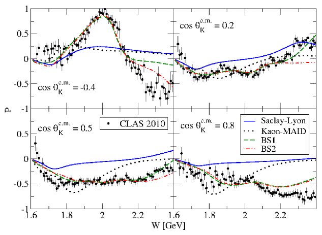
Figure 7: (Color online) Results for energy dependent hyperon polarization are shown for several kaon angles $\theta_{K}^{c.m.}$. Notation of the curves is the same as in the Fig. 3. The CLAS data are from CLAS10 .

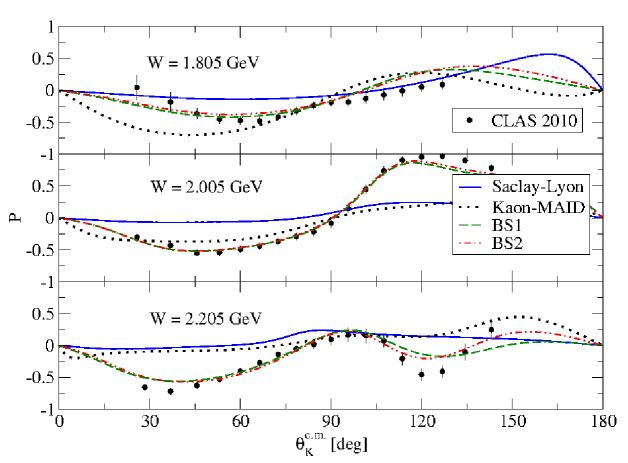
Figure 8: (Color online) Results for the angular dependence of hyperon polarization are shown for several c.m. energies $W$. Notation of the curves is the same as in the Fig. 3. The CLAS data are from CLAS10 .

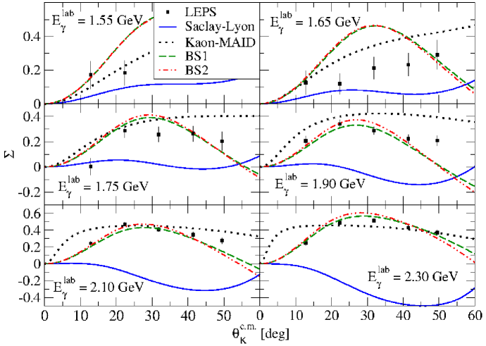
Figure 9: (Color online) Results for the angular dependence of beam asymmetry are shown for several photon lab energies. Notation of the curves is the same as in the Fig. 3. The LEPS data are from LEPS .

In the case of hyperon polarization, the Born terms on their own yield zero contribution but their interference with other terms appears to be important, especially the interference with the nucleon resonances. The models were fitted to the hyperon polarization data from the threshold up to $2.225\,\mbox{GeV}$. In this energy range and mainly in the central-angle region, the data are captured by the BS1 and BS2 models well. On the other hand, the Saclay-Lyon and Kaon-MAID models do not even fit the shape of the data. Note, however, that these old models were not fitted to the hyperon polarization or beam-asymmetry data.

For photon laboratory energy higher than $1.9\,\mbox{GeV}$, the BS1, BS2 and Kaon-MAID models describe the beam-asymmetry data satisfactorily, whereas the Saclay-Lyon model tends to underpredict the data in the whole energy range. Note that the data at lower energies, Fig. 9, have larger relative errors and therefore they cannot restrict the model parameters as much as the data for energies larger that 1.9 GeV.

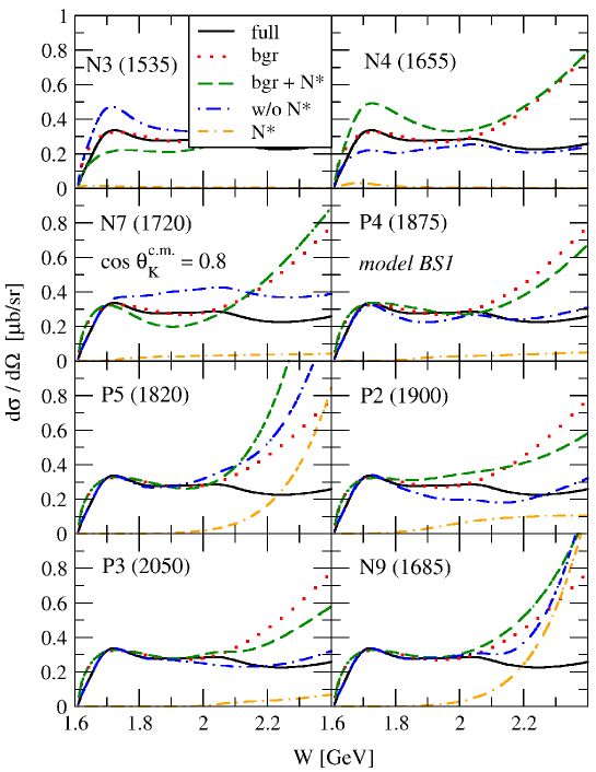
Figure 10: (Color online) Double-polarization observables $C_{x}$ and $C_{z}$ are shown for various kaon angles. Since none of the models were fitted to the $C_{x}$ or $C_{z}$ data, the figure collects merely predictions of the models. Notation of the curves is the same as in the Fig. 3 and the data stem form the CLAS 2005 analysis CLAS05 .

The exchanges of the nucleon resonances in the $s$ channel constitute the resonant structure in the cross section. The effect of a particular resonance strongly depends on the magnitude and sign of its coupling constants, but this effect is hard to estimate in the kaon photoproduction due to overlapping of many resonances and occurrence of the complicated background. In Fig. 10 we show effects of the nucleon resonances in the model BS1 on the forward-angle differential cross section. A contribution of the resonance on its own, in its combination with the background, and a prediction of the full model without the resonance are shown. Comparing the latter with the full result one can infer an importance of the particular resonance in this kinematic region.

In the BS1 model, the contribution of the subthreshold N3 resonance is small, as can be concluded from the relatively small value of its coupling parameter, Tab. 2. However, N3 significantly lowers, by 20 – 30%, the background contribution, which is important in the threshold region where it balances the contribution of N4. Omitting this resonance therefore leads to a growth of the cross section in the threshold region. Similarly, a strong effect is apparent for the N4, N7, and P2 resonances, where the latter two resonances affect the cross section rather at larger energies. On the other hand, the influence of the resonances P3, P5, and N9 on the forward-angle cross section is very small. Their influence is apparent only for energies above 2 GeV. The contributions of the spin-5/2 resonances N9 and P5 start to rise sharply around 2.2 GeV, which instigates the introduction of strong hadron form factors, e.g., the multidipole or multidipole Gauss RPR11 . This effect is not seen for the P3 resonance because it is shifted to higher energies due to its larger mass. Since the BS2 model contains, except for the N6, the same nucleon resonances with very similar values of the coupling parameters, it behaves in a manner similar to the BS1 model.

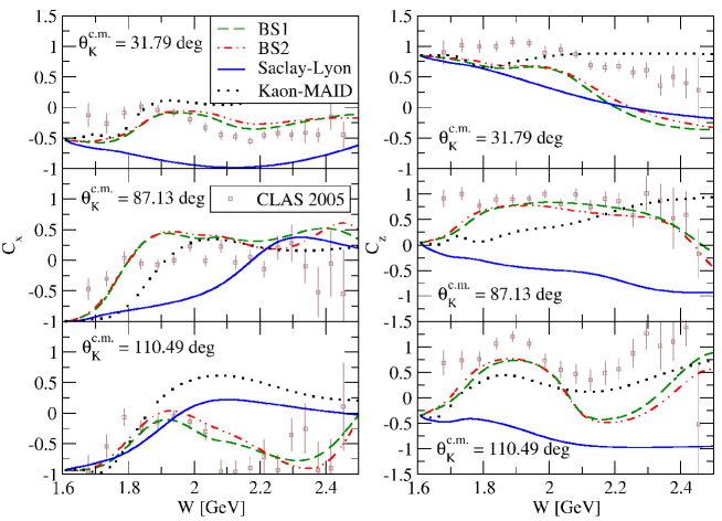
Figure 11: (Color online) Model predictions of the $p(\gamma,K^{+})\Lambda$ total cross section. For comparison, the Gent isobar model (model A) was added as read from Fig. 7 in Ref. Jan01A . Notation of the rest of the curves is the same as in the Fig. 3. Data stem from Fig. 20 in Ref. CLAS05 .

In Fig. 11, the predictions of double-polarization observables $C_{x}$ and $C_{z}$ are shown for various kaon angles. Our new models as well as the well-known Kaon-MAID and Saclay-Lyon models were not fitted to these data sets. Therefore, the figure shows the predictive power of considered models. The Saclay-Lyon model fails to reproduce the $C_{z}$ data for larger kaon angles (whereas the data are positive, the model predictions have opposite sign). The correspondence between other model predictions and the data sets is considerably better: the Kaon-MAID predictions are of the same sign as the data and the BS models capture even the shape of the data.

Our findings on the nucleon resonances agree quite well with the results of the Bayesian analysis which used the Regge-plus-resonance model RPR11 . In this analysis the N3, N4, and N7 resonances were assigned large relative probabilities, 13, 34, and 99, respectively, that they contribute to the kaon photoproduction process. Importance of these resonances was confirmed in our analysis. However, the resonances N9 and P3 were also shown to contribute significantly; their relative probabilities are 16 and 18, respectively, in the RPR-based analysis contrary to our findings which we attribute to the smaller energy window of our analysis (P3 and N9 contribute more at higher energies as shown in Fig. 10). In the Bayesian analysis, it was shown that the N5, N6, and N8 resonances are not required to describe the $\gamma\rm p\longrightarrow K^{+}\Lambda$ data which is also consistent with our conclusions, except for N6 in the BS2 model with the very small coupling parameter $G(N6)=-0.05$. The two-star spin-1/2 resonance $P_{11}(1880)$ (P1) was excluded in our analysis whereas it was included into the set of probable resonances in the Bayesian analysis with the relative probability 11. The spin-5/2 state with near mass, $N^{*}(1860)$ (P5), was assumed in both new models instead. Note that adding P1 into the models does not improve the $\chi^{2}$ too much but it raises the number of considered resonances which we tried to keep as small as possible (according to the principle of the Occam’s razor).

VI Conclusion

In this work, we have presented two new isobar models BS1 and BS2 for the $p(\gamma,K^{+})\Lambda$ process in the energy range from threshold to $W=2.4$ GeV. The models provide satisfactory description of experimental data in the whole energy region and for all kaon angles. Their predictions for the cross sections at small kaon angles, being consistent with the results of the Saclay-Lyon model, suggest that the models can give reasonable values of the cross sections for the hypernucleus production. Construction of a new isobar model utilizing new precision data which could be used as an input in the hypernucleus calculations was one of the aims of this work.

In the construction of the single-channel models based on an effective Lagrangian we have utilized the consistent formalism by Pascalutsa for description of baryon fields with higher spin (3/2 and 5/2 in our case). This formalism ensures that only the physical degrees of freedom contribute in the baryon exchanges. Moreover, it provides regular amplitudes which are especially important for the $u$-channel exchanges allowing the inclusion of hyperon resonances with spin 3/2. These resonances were found to play an important role in description of the background part of the amplitude. They have not been considered in the older isobar models with the inconsistent formalism, except for version C of the Saclay-Lyon model SLA .

The set of selected nucleon resonances with spins 1/2, 3/2, and 5/2 contributing most to the process agrees well with that selected in the Bayesian analysis with the Regge-plus-resonance model by the Gent group. We mostly confirm their result on the structure of the resonant part of the amplitude. The differences for the resonance part, e.g., different forms of the hadron form factor, stem from the fact that we limit our analysis only to the resonance region. As for the missing resonances, we confirm importance of the $P_{13}(1900)$ and $D_{13}(1875)$ states for reasonable data description. We have found, however, that the spin-5/2 state $N^{*}(1860)$, recently included in the PDG Tables, is preferable to the spin-1/2 state $P_{11}(1880)$ included in the Bayesian analysis.

Special attention was paid to the analysis of the background part of the amplitude which is important for a correct description of the forward-angle cross sections. In the background, which is a complicated effect of many various contributions in the isobar approach, the hyperon-resonance exchanges with spin 1/2 and 3/2 together with the Born terms appeared to be important components in the forward- and backward-angle regions, respectively. However, the current extensive data set still does not allow one to select the most significant hyperon resonances in the u channel unambigously.

In the analysis, several forms of the hadron form factors were considered; we chose the dipole and multidipole forms as the most suitable for the data description. The obtained values of the cut-off parameters, around 2 GeV, suggest rather hard form factors.

The free parameters of the models were adjusted by fitting the cross section, hyperon polarization, and the beam asymmetry to new high-quality data from CLAS and LEPS and to older data. The overall number of resonances in the models, 15 and 16, is quite moderate in view of complexity of the kaon photoproduction in comparison with $\pi$ or $\eta$ photoproductions.

It is our desire and purpose to extend the model to study the electroproduction. The presented formalism can be easily extended in this line. Another possibility how to improve the model is to account for the unitarity by making the widths of the nucleon resonances energy-dependent functions as it was done, e.g., in the Kaon-MAID model.

Appendix A Contributions to the invariant amplitude

We consider the process

$$\gamma_{V}(k)+p(p)\rightarrow K^{+}(p_{K})+\Lambda(p_{\Lambda})$$ (35)

with corresponding four-momenta given in the parentheses. The four-momentum of the intermediate particle is denoted by $q$. In the next sections, we summarize the invariant amplitudes with no hadron form factors. These are introduced in the manner shown in Appendix B. The electromagnetic form factors are explicitly included in the Born contributions only. For the rest of the contributions, they are introduced merely by multiplying the coupling parameter with the appropriate electromagnetic form factor.

A.1 Born s-channel

The electromagnetic vertex function reads

$$V^{EM}_{\mu}=F_{1}(k^{2})\gamma_{\mu}+\frac{1-F_{1}(k^{2})}{k^{2}}k_{\mu}\gamma\cdot k+\texttt{i}\frac{F_{2}(k^{2})}{2m_{p}}\sigma_{\mu\nu}k^{\nu},$$ (36)

where $F_{1}(k^{2})$ and $F_{2}(k^{2})$ are standard electromagnetic proton form factors, $F_{1}(0)=1$ and $F_{2}(0)=\kappa_{p}$, where $\kappa_{p}$ is anomalous proton magnetic moment. In the strong vertex, the pseudoscalar coupling is used

$$V_{S}=\texttt{i}g_{K\Lambda p}\gamma_{5}.$$ (37)

The invariant amplitude reads

$$\mathbb{M}_{Bs}=\bar{u}(p_{\Lambda})V_{S}\frac{\not\!p\,+\not\!k+m_{p}}{s-m_{p}^{2}}V_{\mu}^{EM}\varepsilon^{\mu}u(p),$$ (38)

and can be cast into the form (16)

$$\mathbb{M}_{Bs}= \,\,\bar{u}(p_{\Lambda})\gamma_{5}\bigg{[}\mathcal{A}_{1}\mathcal{M}_{1}+\mathcal{A}_{2}\mathcal{M}_{2}+\mathcal{A}_{4}\mathcal{M}_{4}+\mathcal{A}_{6}\mathcal{M}_{6}+g_{K\Lambda p}\frac{k\cdot\varepsilon}{k^{2}}\bigg{]}u(p),$$ (39)

where the last term in the brackets is the gauge-invariance breaking term. One then gets for the scalar amplitudes

$$\mathcal{A}_{1} =\frac{g_{K\Lambda p}}{s-m_{p}^{2}}\left(F_{1}+F_{2}\right),$$ (40a)

$$\mathcal{A}_{2} =2\frac{g_{K\Lambda p}}{s-m_{p}^{2}}F_{1}$$ (40b)

$$\mathcal{A}_{4} =\frac{g_{K\Lambda p}}{s-m_{p}^{2}}\frac{F_{2}}{m_{p}}=-2\mathcal{A}_{6}.$$ (40c)

A.2 Born t-channel

The electromagnetic vertex factor for pseudoscalar mesons $K^{+}$ reads

$$V_{\mu}^{EM}=F(k^{2})(2p_{K}-k)_{\mu}+\frac{1-F(k^{2})}{k^{2}}(2p_{K}-k)\cdot q\,q_{\mu},$$ (41)

where $F(0)=1$. The strong interaction vertex factor is the same as in (37). The invariant amplitude has the form

$$\mathbb{M}_{Bt}=\bar{u}(p_{\Lambda})V_{S}\frac{1}{t-m_{K}^{2}}V_{\mu}^{EM}\varepsilon^{\mu}u(p),$$ (42)

which can again be cast to the compact form

$$\mathbb{M}_{Bt}=\bar{u}(p_{\Lambda})\gamma_{5}\left[\mathcal{A}_{2}\mathcal{M}_{2}+\mathcal{A}_{3}\mathcal{M}_{3}-g_{K\Lambda p}\frac{k\cdot\varepsilon}{k^{2}}\right]u(p),$$ (43)

where the last term in the brackets is the same gauge-invariance breaking term as in the Born s-channel contribution, Eq. (39), but with the opposite sign. Therefore, these two terms cancel in the total amplitude of the process and the gauge invariance remains preserved. There are only two nonzero scalar amplitudes

$$\mathcal{A}_{2}=-\mathcal{A}_{3}=2\frac{g_{K\Lambda p}}{t-m_{K}^{2}}F.$$ (44)

A.3 Born u-channel

The electromagnetic $\gamma\Lambda\Lambda$ vertex factor has the form

$$V_{\mu}^{EM}=F_{1}(k^{2})\left[\gamma_{\mu}-\frac{k_{\mu}\gamma\cdot k}{k^{2}}\right]+\texttt{i}\frac{F_{2}(k^{2})}{2m_{\Lambda}}\sigma_{\mu\nu}k^{\nu},$$ (45)

where $F_{1}(0)=0$ and $F_{2}(0)=\kappa_{\Lambda}$. The strong interaction vertex factor is the same as in (37). The Born u-channel amplitude reads

$$\mathbb{M}_{Bu}=\bar{u}(p_{\Lambda})V_{\mu}^{EM}\frac{\not\!p_{\Lambda}-\not\!k+m_{\Lambda}}{u-m_{\Lambda}^{2}}V_{S}\,\varepsilon^{\mu}u(p)$$ (46)

and the scalar amplitudes $\mathcal{A}_{j}$ are

$$\mathcal{A}_{1}= \frac{g_{K\Lambda p}}{u-m_{\Lambda}^{2}}(F_{1}+F_{2}),$$ (47a)

$$\mathcal{A}_{3}= 2\frac{g_{K\Lambda p}}{u-m_{\Lambda}^{2}}F_{1},$$ (47b)

$$\mathcal{A}_{5}= \frac{g_{K\Lambda p}}{u-m_{\Lambda}^{2}}\frac{F_{2}}{m_{\Lambda}}=2\mathcal{A}_{6}.$$ (47c)

A.4 Non-Born s-channel: $N^{*}(1/2^{\pm})$ exchange

The amplitude for this contribution has the form

$$\mathbb{M}^{N^{*}(1/2)}_{NBs}= \,\,\texttt{i}\bar{u}(p_{\Lambda})\,g_{K\Lambda R}\,\gamma_{5}\,\Gamma\frac{\not\!p+\not\!k+m_{R}}{s-m_{R}^{2}+\texttt{i}m_{R}\Gamma_{R}}\,\frac{\mu_{pR}}{m_{p}+m_{R}}\sigma^{\mu\nu}k_{\nu}\Gamma\varepsilon_{\mu}u(p).$$ (48)

In the case of nucleon resonances we have to distinguish between the positive and negative parity resonances. This can be done by using $\Gamma$ in the form

$$\Gamma=\begin{cases}1,&P=+1,\\ \gamma_{5},&P=-1,\\ \end{cases}$$ (49)

The scalar amplitudes are

$$\mathcal{A}_{1} =\frac{g_{K\Lambda R}}{s-m_{R}^{2}+\texttt{i}m_{R}\Gamma_{R}}\frac{m_{R}\pm m_{p}}{m_{R}+m_{p}}\mu_{pR},$$ (50a)

$$\mathcal{A}_{4} =\pm\frac{g_{K\Lambda R}}{s-m_{R}^{2}+\texttt{i}m_{R}\Gamma_{R}}\frac{2\mu_{pR}}{m_{p}+m_{R}},$$ (50b)

$$\mathcal{A}_{6} =-\frac{1}{2}\mathcal{A}_{4},$$ (50c)

where the upper (lower) sign corresponds with the case of positive (negative) parity of the nucleon resonance.

A.5 Non-Born s-channel: $N^{*}(3/2^{\pm})$ exchange

The amplitude of the spin-3/2 contribution reads

$$\mathbb{M}_{NBs}^{N^{*}(3/2)}= \,\,\bar{u}(p_{\Lambda})\,\Gamma\,\frac{\texttt{i}f}{m_{R}m_{K}}\,\epsilon_{\mu\nu\lambda\rho}\,\gamma_{5}\,\gamma^{\lambda}q^{\mu}p_{K}^{\rho}\,\frac{\not\!q+m_{R}}{s-m^{2}_{R}+\texttt{i}m_{R}\Gamma_{R}}\,\left(g^{\nu\beta}-\frac{1}{3}\gamma^{\nu}\gamma^{\beta}\right)$$ (51)

$$\times\frac{1}{m_{R}(m_{R}+m_{p})}\,\Big{(}g_{1}q^{\alpha}F_{\alpha\beta}+g_{2}\not\!q\,F_{\beta\alpha}\,\gamma^{\alpha}-g_{2}\gamma_{\beta}\,q^{\alpha}\,F_{\alpha\tau}\,\gamma^{\tau}\Big{)}\,\Gamma\,\gamma_{5}\,u(p),$$

where $g_{1}$ and $g_{2}$ are the electromagnetic coupling constants and $f$ is the strong coupling constant. Casting the amplitude to the compact form (16), the individual scalar amplitudes $\mathcal{A}_{j}$ read

$$\begin{split}\mathcal{A}^{\prime}_{1}={}&-\frac{G_{1}}{3}(q\cdot p_{\Lambda}\pm m_{R}m_{\Lambda})\,q\cdot k+\frac{G_{2}}{3}(2s\,q\cdot p_{\Lambda}-3s\,k\cdot p_{\Lambda}+2s\,m_{p}m_{\Lambda}\mp m_{R}m_{\Lambda}\,q\cdot k\pm 2s\,m_{R}m_{\Lambda}\\ &\pm 2m_{p}m_{R}q\cdot p_{\Lambda}+2q\cdot p_{\Lambda}\,q\cdot k),\end{split}$$ (52a)

$$\begin{split}\mathcal{A}^{\prime}_{2}={}&G_{1}\bigg{[}s\,k\cdot p_{\Lambda}\mp m_{R}m_{p}\,k\cdot p_{\Lambda}-\frac{1}{3}q\cdot p_{\Lambda}\,k^{2}\mp\frac{1}{3}m_{R}m_{\Lambda}k^{2}\bigg{]}+G_{2}\left[-2s\,k\cdot p_{\Lambda}\mp\frac{1}{3}m_{\Lambda}m_{R}k^{2}+\frac{2}{3}k^{2}\,q\cdot p_{\Lambda}\right],\end{split}$$ (52b)

$$\begin{split}\mathcal{A}^{\prime}_{3}={}&G_{1}(\pm m_{R}m_{p}-s)q\cdot k+G_{2}(2q\cdot k-k^{2})s,\end{split}$$ (52c)

$$\begin{split}\mathcal{A}^{\prime}_{4}={}&G_{1}\bigg{[}-\frac{1}{3}s\,m_{\Lambda}+\frac{1}{3}(m_{p}\mp m_{R})\,q\cdot p_{\Lambda}\pm\frac{1}{3}m_{\Lambda}m_{p}m_{R}\pm m_{R}\,k\cdot p_{\Lambda}\bigg{]}\\ &-G_{2}\left[-s\,m_{\Lambda}\mp\frac{1}{3}m_{\Lambda}m_{p}m_{R}+\frac{2}{3}m_{p}\,q\cdot p_{\Lambda}\right],\end{split}$$ (52d)

$$\begin{split}\mathcal{A}^{\prime}_{5}={}&\mp G_{1}m_{R}\,q\cdot k+G_{2}(\pm m_{R}+m_{p})s,\end{split}$$ (52e)

$$\begin{split}\mathcal{A}^{\prime}_{6}={}&G_{1}\bigg{[}\mp\frac{1}{3}m_{\Lambda}m_{p}m_{R}\mp m_{R}\,k\cdot p_{\Lambda}+\frac{1}{3}m_{\Lambda}s-\frac{1}{3}q\cdot p_{\Lambda}\,(m_{p}\mp m_{R})\bigg{]}\\ &+G_{2}\left[-\frac{1}{3}m_{\Lambda}s\mp\frac{1}{3}m_{\Lambda}m_{p}m_{R}+\frac{2}{3}q\cdot p_{\Lambda}\,(m_{p}\pm m_{R})\right],\end{split}$$ (52f)

where the coupling parameters $G_{1}$ and $G_{2}$ are given in Eq. (33) and the upper (lower) sign corresponds with the case of positive (negative) parity of the nucleon resonance.

Each amplitude $\mathcal{A}^{\prime}_{i},\,i=1,\ldots,6$, has to be multiplied by the propagator denominator

$$\mathcal{A}_{i}=\frac{1}{s-m_{R}^{2}+\texttt{i}m_{R}\Gamma_{R}}\mathcal{A}^{\prime}_{i}.$$ (53)

A.6 Non-Born $s$-channel: $N^{*}(5/2^{\pm})$ exchange

The amplitude for the $N^{*}(5/2^{\pm})$ exchange reads

$$\mathbb{M}_{NBS}^{N^{*}(5/2)}= -\frac{f}{m_{K}^{4}}\bar{u}(p_{\Lambda})\gamma_{5}\Gamma\,q^{2}p_{K}^{\mu}p_{K}^{\nu}\frac{\not\!q+m_{R}}{s-m_{R}^{2}+\texttt{i}m_{R}\Gamma_{R}}$$ (54)

$$\times\mathcal{P}_{\mu\nu,\lambda\rho}(q)\,q^{2}\,p^{\lambda}\bigg{[}\frac{g_{1}}{(2m_{p})^{4}}\,\gamma_{\alpha}\,F^{\alpha\rho}+\frac{g_{2}}{(2m_{p})^{5}}p_{\alpha}\,F^{\alpha\rho}\bigg{]}\Gamma\,u(p)$$

Casting the amplitude to the compact form (16), the scalar amplitudes then read

$$\begin{split}\mathcal{A}^{\prime}_{1}={}&G_{1}\bigg{\{}\mp Q_{p_{\Lambda}p}Q_{kp_{\Lambda}}\pm\frac{1}{5}Q_{p_{\Lambda}p_{\Lambda}}Q_{kp}-\frac{1}{5}Q_{kp_{\Lambda}}(B\,q\cdot p+Cm_{p})+\frac{1}{5}Q_{p_{\Lambda}p}[2Cm_{p}+(2s-q\cdot k)B]\bigg{\}}\\ &-\frac{G_{2}}{5}Q_{p_{\Lambda}p}Ck\cdot p,\end{split}$$ (55a)

$$\begin{split}\mathcal{A}^{\prime}_{2}={}&G_{1}\bigg{\{}\pm Q_{p_{\Lambda}p}(k^{2}q\cdot p_{\Lambda}-2sk\cdot p_{\Lambda})\mp\frac{1}{5}Q_{p_{\Lambda}p_{\Lambda}}k^{2}(q\cdot p+s)-\frac{1}{5}[\mp 2q\cdot p_{\Lambda}\,k\cdot p_{\Lambda}\,q\cdot ks\pm k^{2}(q\cdot p_{\Lambda})^{2}(q\cdot k+s)\\ &+2sm_{R}m_{\Lambda}k\cdot p_{\Lambda}q\cdot k-m_{R}m_{\Lambda}k^{2}q\cdot p_{\Lambda}(q\cdot k+s)+Cm_{p}k^{2}q\cdot p_{\Lambda}]-\frac{1}{5}Q_{p_{\Lambda}p}k^{2}B\bigg{\}}\\ &+G_{2}\bigg{\{}(m_{R}\pm m_{p})Q_{p_{\Lambda}p}D-\frac{1}{5}(m_{R}\pm m_{p})k^{2}q\cdot pQ_{p_{\Lambda}p_{\Lambda}}\\ &+\frac{1}{5}(sk\cdot p_{\Lambda}-k^{2}q\cdot p_{\Lambda})(Bm_{p}q\cdot k-Ck\cdot p)-\frac{1}{5}Q_{p_{\Lambda}p}Bm_{p}k^{2}\bigg{\}},\end{split}$$ (55b)

$$\begin{split}\mathcal{A}^{\prime}_{3}={}&G_{1}\bigg{\{}\pm sQ_{p_{\Lambda}p}(2k\cdot p+k^{2})-\frac{1}{5}s[(2k\cdot p\,q\cdot k-k^{2}q\cdot p)B-m_{p}k^{2}C]\bigg{\}}\\ &+G_{2}\bigg{\{}s(m_{R}\pm m_{p})k\cdot p\,Q_{p_{\Lambda}p}-\frac{1}{5}sk\cdot p(Bm_{p}q\cdot k-Ck\cdot p)\bigg{\}},\end{split}$$ (55c)

$$\begin{split}\mathcal{A}^{\prime}_{4}={}&G_{1}\bigg{\{}\frac{1}{5}(m_{R}\mp m_{p})q\cdot kQ_{p_{\Lambda}p_{\Lambda}}-AQ_{p_{\Lambda}p}\\ &+\frac{1}{5}\{q\cdot p_{\Lambda}[Bm_{p}q\cdot k+C(2k^{2}+k\cdot p)+2s\,m_{R}k\cdot p_{\Lambda}]\pm 2k\cdot p_{\Lambda}s^{2}m_{\Lambda}\}\\ &-\frac{1}{5}Q_{p_{\Lambda}p}[m_{\Lambda}(m_{R}m_{p}\mp 3s)+(3m_{R}\mp m_{p})q\cdot p_{\Lambda}]\bigg{\}}+G_{2}\bigg{\{}\pm\frac{1}{5}k^{2}q\cdot pQ_{p_{\Lambda}p_{\Lambda}}\mp DQ_{p_{\Lambda}p}+\frac{1}{5}DE\\ &-\frac{1}{5}Q_{p_{\Lambda}p}[m_{R}m_{\Lambda}(k^{2}\mp s)+q\cdot p_{\Lambda}(m_{R}m_{p}\mp k^{2})\pm s(q\cdot p_{\Lambda}-m_{\Lambda}m_{p})]\bigg{\}},\end{split}$$ (55d)

$$\begin{split}\mathcal{A}^{\prime}_{5}={}&G_{1}\bigg{\{}s(\pm m_{p}-m_{R})Q_{p_{\Lambda}p}-\frac{1}{5}s(Bm_{p}q\cdot k-Ck\cdot p)\bigg{\}}+G_{2}\bigg{\{}\pm sk\cdot p\,Q_{p_{\Lambda}p}+\frac{1}{5}Esk\cdot p\bigg{\}},\end{split}$$ (55e)

$$\begin{split}\mathcal{A}^{\prime}_{6}={}&G_{1}\bigg{\{}AQ_{p_{\Lambda}p}-\frac{1}{5}q\cdot p(\pm m_{p}-m_{R})Q_{p_{\Lambda}p_{\Lambda}}-\frac{1}{5}q\cdot p_{\Lambda}(Bm_{p}q\cdot k-Ck\cdot p)-\frac{1}{5}Q_{p_{\Lambda}p}[m_{\Lambda}(\pm s-m_{R}m_{p})+A]\bigg{\}}\\ &-G_{2}\bigg{\{}\pm q\cdot p_{\Lambda}\,k\cdot p\,Q_{p_{\Lambda}p}\pm\frac{1}{5}q\cdot p\,k\cdot p\,Q_{p_{\Lambda}p_{\Lambda}}+\frac{1}{5}q\cdot p_{\Lambda}\,k\cdot pE+\frac{1}{5}Q_{p_{\Lambda}p}B\,k\cdot p\bigg{\}},\end{split}$$ (55f)

where the coupling parameters $G_{1}$ and $G_{2}$ are given as in (34) and

$$A={} q\cdot p_{\Lambda}(\pm m_{p}-m_{R}),$$ (56a)

$$B={} \pm q\cdot p_{\Lambda}-m_{\Lambda}m_{R},$$ (56b)

$$C={} \pm sm_{\Lambda}-m_{R}\,q\cdot p_{\Lambda},$$ (56c)

$$D={} k^{2}\,q\cdot p_{\Lambda}-s\,k\cdot p_{\Lambda},$$ (56d)

$$E={} m_{p}C-q\cdot p\,B,$$ (56e)

where the upper (lower) sign corresponds with the case of positive (negative) parity of the nucleon resonance.

The terms $Q_{p_{\Lambda}p},\,Q_{kp_{\Lambda}},\,Q_{p_{\Lambda}p_{\Lambda}}$ and $Q_{kp}$ include four-momenta products given by the general prescription

$$Q_{XY}=s\,X\cdot Y-X\cdot q\,Y\cdot q,$$ (57)

the notation of four-momenta is given in (35).

Each amplitude $\mathcal{A}^{\prime}_{i},\,i=1,\ldots,6$, has to be multiplied by the propagator denominator as in Eq. (53).

A.7 Non-Born t-channel: $K_{1}(1270)$ and $K^{*}(892)$ exchange

The amplitude for the pseudovector meson $K_{1}(1270)$ ($J^{\pi}=1^{+}$) exchange reads

$$\mathbb{M}_{NBt}^{K_{1}}= \,\,\bar{u}(p_{\Lambda})\frac{g}{m}[g_{\alpha\mu}\,k\cdot(p-p_{\Lambda})-k_{\alpha}(p-p_{\Lambda})_{\mu}]\,\frac{\left(-g^{\alpha\lambda}+(p-p_{\Lambda})^{\alpha}(p-p_{\Lambda})^{\lambda}/m_{K_{1}}^{2}\right)}{t-m_{K_{1}}^{2}+\texttt{i}m_{K_{1}}\Gamma_{K_{1}}}$$ (58)

$$\times\left[f_{V}\gamma_{\lambda}\gamma_{5}+\frac{f_{T}}{m_{\Lambda}+m_{p}}(\not\!p_{\Lambda}-\not\!p)\gamma_{\lambda}\gamma_{5}\right]\varepsilon^{\mu}u(p).$$

And the scalar amplitudes $\mathcal{A}_{j}$ are given as

$$\mathcal{A}_{2} =\frac{-2G_{T}}{(m_{\Lambda}+m_{p})(t-m_{K_{1}}^{2}+\texttt{i}m_{K_{1}}\Gamma_{K_{1}})}\,p_{\Lambda}\cdot k,$$ (59a)

$$\mathcal{A}_{3} =\frac{2G_{T}}{(m_{\Lambda}+m_{p})(t-m_{K_{1}}^{2}+\texttt{i}m_{K_{1}}\Gamma_{K_{1}})}\,p\cdot k,$$ (59b)

$$\mathcal{A}_{4} =\frac{G_{V}+G_{T}(m_{\Lambda}-m_{p})/(m_{\Lambda}+m_{p})}{t-m_{K_{1}}^{2}+\texttt{i}m_{K_{1}}\Gamma_{K_{1}}},$$ (59c)

$$\mathcal{A}_{5} =-\mathcal{A}_{4}.$$ (59d)

with $G_{V,T}=gf_{V,T}/m$. The mass scale $m$ is arbitrarily chosen as $1\,\mbox{GeV}$.

The vector meson $K^{*}(892)$ ($J^{\pi}=1^{-}$) exchange amplitude is

$$\mathbb{M}_{NBt}^{K^{*}}= \,\,\texttt{i}\bar{u}(p_{\Lambda})\frac{g}{m}\epsilon^{\mu\nu\alpha\beta}k_{\alpha}(p_{\Lambda}-p)_{\beta}\,\frac{\left(-g_{\nu\sigma}+(p-p_{\Lambda})_{\nu}(p-p_{\Lambda})_{\sigma}/m_{K^{*}}^{2}\right)}{t-m_{K^{*}}^{2}+\texttt{i}m_{K^{*}}\Gamma_{K^{*}}}$$ (60)

$$\times\left[f_{V}\gamma^{\sigma}+\frac{f_{T}}{m_{\Lambda}+m_{p}}(\not\!p_{\Lambda}-\not\!p)\gamma^{\sigma}\right]\varepsilon_{\mu}u(p).$$

The scalar amplitudes are given as

$$\mathcal{A}_{1} =\frac{G_{V}(m_{\Lambda}+m_{p})+G_{T}\,t/(m_{\Lambda}+m_{p})}{t-m_{K^{*}}^{2}+\texttt{i}m_{K^{*}}\Gamma_{K^{*}}},$$ (61a)

$$\mathcal{A}_{2} =\frac{2k\cdot p_{\Lambda}\,G_{T}}{(m_{\Lambda}+m_{p})(t-m_{K^{*}}^{2}+\texttt{i}m_{K^{*}}\Gamma_{K^{*}})},$$ (61b)

$$\mathcal{A}_{3} =\frac{-2k\cdot p\,G_{T}}{(m_{\Lambda}+m_{p})(t-m_{K^{*}}^{2}+\texttt{i}m_{K^{*}}\Gamma_{K^{*}})},$$ (61c)

$$\mathcal{A}_{4} =\frac{G_{V}-G_{T}(m_{\Lambda}-m_{p})/(m_{\Lambda}+m_{p})}{t-m_{K^{*}}^{2}+\texttt{i}m_{K^{*}}\Gamma_{K^{*}}},$$ (61d)

$$\mathcal{A}_{5} =\frac{G_{V}+G_{T}(m_{\Lambda}-m_{p})/(m_{\Lambda}+m_{p})}{t-m_{K^{*}}^{2}+\texttt{i}m_{K^{*}}\Gamma_{K^{*}}},$$ (61e)

with $G_{V,T}=gf_{V,T}/m$. As in the pseudovector case, the mass $m$ is arbitrarily chosen to be $1\,\mbox{GeV}$.

A.8 Non-Born u-channel: $Y^{*}(1/2^{\pm})$ exchange

The non-Born amplitude for the $Y^{*}(1/2^{\pm})$ exchange is

$$\mathbb{M}_{NBu}^{Y^{*}(1/2)}= \,\,\texttt{i}\bar{u}(p_{\Lambda})\frac{\kappa_{\Lambda R}}{m_{\Lambda}+m_{R}}\sigma^{\mu\nu}k_{\nu}\Gamma\,\frac{\not\!p_{\Lambda}-\not\!k+m_{R}}{u-m_{R}+\texttt{i}m_{R}\Gamma_{R}}g_{K\Lambda^{*}p}\gamma_{5}\Gamma\varepsilon_{\mu}u(p),$$ (62)

with $\Gamma$ defined as in (49).

The scalar amplitudes $\mathcal{A}_{j}$ are then

$$\mathcal{A}_{1} =\frac{g_{K\Lambda^{*}p}}{u-m_{R}^{2}+\texttt{i}m_{R}\Gamma_{R}}\frac{m_{R}\pm m_{\Lambda}}{m_{R}+m_{\Lambda}}\kappa_{\Lambda R},$$ (63a)

$$\mathcal{A}_{5} =\pm\frac{g_{K\Lambda^{*}p}}{u-m_{R}^{2}+\texttt{i}m_{R}\Gamma_{R}}\frac{2\kappa_{\Lambda R}}{m_{\Lambda}+m_{R}},$$ (63b)

$$\mathcal{A}_{6} =\frac{1}{2}\mathcal{A}_{5},$$ (63c)

where the upper (lower) sign corresponds with the positive (negative) parity of the resonance.

A.9 Non-Born u-channel: $Y^{*}(3/2^{\pm})$ exchange

The amplitude for the $Y^{*}(3/2^{\pm})$ exchange in the u-channel reads

$$\mathbb{M}_{NBu}^{Y^{*}(3/2)}= \,\,\,\bar{u}(p_{\Lambda})\,\Gamma\,\gamma_{5}\,\frac{1}{m_{R}(m_{R}+m_{\Lambda})}\Big{[}g_{1}\,q^{\alpha}\,F_{\alpha\beta}+g_{2}\Big{(}\not\!q\,F_{\beta\alpha}\gamma^{\alpha}-\gamma_{\beta}\,q^{\alpha}\,F_{\alpha\rho}\,\gamma^{\rho}\Big{)}\Big{]}$$ (64)

$$\times\frac{\not\!q+m_{R}}{u-m_{R}^{2}+\texttt{i}m_{R}\Gamma_{R}}\left(g^{\beta\nu}-\frac{1}{3}\gamma^{\beta}\gamma^{\nu}\right)\,\Gamma\frac{\texttt{i}f}{m_{R}m_{K}}\,\epsilon_{\mu\nu\lambda\rho}\,\gamma_{5}\gamma^{\lambda}q^{\mu}p_{K}^{\rho}\,u(p),$$

Casting the amplitude to the compact form, the scalar amplitudes are given as

$$\begin{split}\mathcal{A}^{\prime}_{1}={}&-\frac{1}{3}G_{1}q\cdot k\,(\pm m_{R}m_{p}+q\cdot p)\\ &+\frac{1}{3}G_{2}\left[\pm 5m_{R}m_{p}\,q\cdot k\pm 2m_{R}m_{p}u+2q\cdot p\,q\cdot k\pm 2m_{R}m_{\Lambda}\,q\cdot p+2u\,q\cdot p+2m_{\Lambda}m_{p}u+3u\,p\cdot k\right],\end{split}$$ (65a)

$$\begin{split}\mathcal{A}^{\prime}_{2}={}&G_{1}q\cdot k\,(\pm m_{R}m_{\Lambda}-u)+G_{2}(2q\cdot k\,u-uk^{2}\mp 4m_{R}m_{\Lambda}\,q\cdot k),\end{split}$$ (65b)

$$\begin{split}\mathcal{A}^{\prime}_{3}={}&\,\,G_{1}\left\{\frac{1}{3}k^{2}(\pm m_{p}m_{R}+q\cdot p)+p\cdot k\,(u\mp m_{R}m_{\Lambda})\right\}+G_{2}\left[\pm 4m_{R}m_{\Lambda}\,p\cdot k\mp\frac{5}{3}m_{R}m_{p}k^{2}-\frac{2}{3}q\cdot p\,k^{2}-2p\cdot k\,u\right],\end{split}$$ (65c)

$$\begin{split}\mathcal{A}^{\prime}_{4}={}&\mp G_{1}m_{R}\,q\cdot k+G_{2}[\pm 4m_{R}\,q\cdot k+u(\pm m_{R}+m_{\Lambda})],\end{split}$$ (65d)

$$\begin{split}\mathcal{A}^{\prime}_{5}={}&\,\,\frac{1}{3}G_{1}[q\cdot p\,(\pm m_{R}-m_{\Lambda})\mp m_{R}m_{p}m_{\Lambda}+u\,m_{p}\pm 3m_{R}\,p\cdot k]\\ &+G_{2}\left[\pm\frac{5}{3}m_{R}m_{p}m_{\Lambda}\mp 4m_{R}\,p\cdot k-\frac{1}{3}u\,m_{p}+\frac{2}{3}m_{\Lambda}\,q\cdot p\mp\frac{4}{3}m_{R}\,q\cdot p\right],\end{split}$$ (65e)

$$\begin{split}\mathcal{A}^{\prime}_{6}={}&\,\,\frac{1}{3}G_{1}[q\cdot p\,(\pm m_{R}-m_{\Lambda})\mp m_{R}m_{p}m_{\Lambda}+u\,m_{p}\pm 3m_{R}\,p\cdot k]\\ &+G_{2}\left[\pm\frac{5}{3}m_{R}m_{p}m_{\Lambda}\mp 4m_{R}\,p\cdot k\mp 2m_{R}\,q\cdot p-u\,m_{p}+\frac{2}{3}m_{\Lambda}\,q\cdot p\right],\end{split}$$ (65f)

where $G_{1,2}$ are given as in (33) with $m_{p}$ replaced by $m_{\Lambda}$ and the upper (lower) sign corresponds with the case of positive (negative) parity of the hyperon resonance. Each amplitude $\mathcal{A}^{\prime}_{i},\,i=1,\ldots,6$, has to be multiplied by the propagator denominator

$$\mathcal{A}_{i}=\frac{1}{u-m_{R}^{2}+\texttt{i}m_{R}\Gamma_{R}}\mathcal{A}^{\prime}_{i}.$$ (66)

Appendix B Inclusion of hadron form factors and the gauge-invariance restoration

The hadron form factors are included in a similar manner as the electromagnetic ones for a gauge-invariant vertex: it is sufficient to multiply the coupling parameter with the hadron form factor, $G\to FG$, where $G$ and $F$ are the coupling parameter and hadron form factor, respectively.

With the introduction of hadron form factors the gauge non-invariant terms in the s- and t-channel Born contributions no longer cancel each other and the gauge invariance is lost. In order to restore it, the contact term

$$\mathbb{M}_{contact}= -g_{K\Lambda p}\bar{u}_{\Lambda}(p_{\Lambda})\gamma_{5}\bigg{[}\frac{2p^{\mu}+\not\!k\gamma^{\mu}}{s-m_{p}^{2}}(\hat{F}_{DW}-F_{s})+\frac{2p_{K}^{\mu}}{t-m_{K}^{2}}(\hat{F}_{DW}-F_{t})\bigg{]}u_{p}(p)\varepsilon_{\mu},$$ (67)

is implemented. For $\hat{F}_{DW}$ the form

$$\hat{F}_{DW}=F_{s}(s)+F_{t}(t)-F_{s}(s)F_{t}(t),$$ (68)

introduced by Davidson and Workman DW is used. In the definition (68) it holds that $F_{s}(s=m_{p}^{2})=F_{t}(t=m_{K}^{2})=1$ and $\hat{F}_{DW}(s=m_{p}^{2},t)=\hat{F}_{DW}(s,t=m_{K}^{2})=1$, which prevents the poles in the contact-term contribution (67) from being reached.

References

- (1) S. Capstick and W. Roberts, Prog. Part. Nucl. Phys. 45, S241 (2000).
- (2) U. Loring, B. C. Metsch, and H. R. Petry, Eur. Phys. J. A 10, 395 (2001); Eur. Phys. J. A 10, 447 (2001).
- (3) P. Bydžovský, M. Sotona, T. Motoba, K. Itonaga, K. Ogawa, and O. Hashimoto, Nucl. Phys. A 881, 187 (2012); T. Motoba, P. Bydžovský, M. Sotona, and K. Itonaga, Prog. Theor. Phys. Suppl. 185, 224 (2010).
- (4) P. Bydžovský and T. Mart, Phys. Rev. C 76, 065202 (2007).
- (5) R. A. Adelseck and B. Saghai, Phys. Rev. C 42, 108 (1990).
- (6) J. C. David, C. Fayard, G.-H. Lamot, and B. Saghai, Phys. Rev. C 53, 2613 (1996).
- (7) T. Mizutani, C. Fayard, G.-H. Lamot, and B. Saghai, Phys. Rev. C 58, 75 (1998).
- (8) S. Janssen, J. Ryckebusch, D. Debruyne, and T. Van Cauteren, Phys. Rev. C 65, 015201 (2001).
- (9) S. Janssen, J. Ryckebusch, W. Van Nespen, D. Debruyne, and T. Van Cauteren, Eur. Phys. J. A 11, 105 (2001).
- (10) S. Janssen, D. G. Ireland, J. Ryckebusch, Phys. Lett. B 562, 51 (2003).
- (11) R. A. Williams, Chueng-Ryong Ji, and S. R. Cotanch, Phys. Rev. C 46, 1617 (1992).
- (12) P. Bydžovský, F. Cusanno, S. Frullani, F. Garibaldi, M. Iodice, M. Sotona, and G. M. Urciuoli, nucl-th/0305039.
- (13) R. Bradford et al., Phys.Rev. C 73 (2006) 035202, J. W. C. McNabb et al., Phys. Rev. C69, 042201(R) (2004).
- (14) M. E. McCracken et al., Phys. Rev. C 81 (2010) 025201.
- (15) M. Sumihama et al., Phys. Rev. C 73 (2006) 035214.
- (16) A. Lleres et al., Eur. Phys. J. A 31, 79 (2007); A. Lleres et al., Eur. Phys. J. A 39, 149 (2009).
- (17) K.-H. Glander et al., Eur. Phys. J. A 19, 251 (2004).
- (18) V. Shklyar, H. Lenske, and U. Mosel, Phys. Rev. C 72, 015210 (2005); R. Shyam, O. Scholten, and H. Lenske, Phys. Rev. C 81, 015204 (2010).
- (19) B. Julia-Diaz, B. Saghai, T.-S. H. Lee, and F. Tabakin, Phys. Rev. C 73, 055204 (2006).
- (20) A. V. Anisovich, V. Kleber, E. Klempt, V. A. Nikonov, A. V. Sarantsev, and U. Thoma, Eur. Phys. J. A 34, 243 (2007).
- (21) B. Borasoy, P. C. Bruns, U.-G. Meissner, and R. Nissler, Eur. Phys. J. A 34, 161 (2007).
- (22) T. Corthals, J. Ryckebusch, and T. Van Cauteren, Phys. Rev. C 73, 045207 (2006); T. Corthals, T. Van Cauteren, J. Ryckebusch, and D. G. Ireland, Phys. Rev. C 75, 045204 (2007); T. Corthals, T. Van Cauteren, P. Vancraeyveld, J. Ryckebusch, and D. G. Ireland, Phys. Lett. B656, 186 (2007).
- (23) T. Mart and A. Sulaksono, Phys. Rev. C 74, 055203 (2006).
- (24) T. Mart, Phys. Rev C 82, 025209 (2010).
- (25) O. V. Maxwell, Phys. Rev. C 76, 014621 (2007); A. de la Puente, O. V. Maxwell, and B. A. Raue, Phys. Rev. C 80, 065205 (2009).
- (26) Zhenping Li, Phys. Rev. C 52, 1648 (1995); Zhenping Li, Hongxing Ye, Minghui Lu, Phys. Rev. C 56, 1099 (1997).
- (27) D. Lu, R. H. Landau, and S. C. Phatak, Phys. Rev. C 52, 1662 (1995).
- (28) G. R. Farrar, K. Huleihel, and H. Zhang, Nucl. Phys. B 349, 655 (1991).
- (29) S. Steininger and U.-G. Meissner, Phys. Lett. B 391, 446 (1997).
- (30) T. Mart and C. Bennhold, Phys. Rev. C 61, 012201(R) (1999); T. Mart, Phys. Rev. C 62, 038201 (2000); T. Mart, C. Bennhold, H. Haberzettl, and L. Tiator, http://www.kph.uni-mainz.de/MAID/kaon/kaonmaid.html.
- (31) H. Thom, Phys. Rev. 151, 1322 (1966).
- (32) M. Benmerrouche, R. M. Davidson, and N. C. Mukhopadhyay, Phys. Rev. C 39, 2339 (1989).
- (33) V. Pascalutsa, Phys. Rev. D 58, 096002 (1998).
- (34) T. Vrancx, L. De Cruz, J. Ryckebusch, and P. Vancraeyveld, Phys. Rev. C 84, 045201 (2011).
- (35) L. De Cruz, T. Vrancx, P. Vancraeyveld, and J. Ryckebusch, Phys. Rev. Lett. 108 (2012) 182002; L. De Cruz, J. Ryckebusch, T. Vrancx, P. Vancraeyveld, Phys. Rev. C 86, 015212 (2012).
- (36) M. Guidal, J.-M. Laget, and M. Vanderhaeghen, Nucl. Phys. A 627, 645 (1997).
- (37) M. Sotona and S. Frullani, Prog. Theor. Phys. Suppl. 117, 151 (1994).
- (38) S. S. Hsiao, D. H. Lu, and S. N. Yang, Phys. Rev. C 61, 068201 (2000); B. Han, M. Cheoun, K. Kim, and I.-T. Cheon, Nucl. Phys. A 691, 713 (2001).
- (39) V. Pascalutsa and R. Timmermans, Phys. Rev. C 60, 042201.
- (40) T. Mart, Phys. Rev. C 87, 042201 (2013).
- (41) K. A. Olive et al. (Particle Data Group), Chin. Phys. C, 38, 090001 (2014).
- (42) T. Mart and N. Nurhadiansyah, Few-Body Syst., 54, 1729 (2012).
- (43) G. Knöchlein, D. Drechsel, and L. Tiator, Z. Phys. A 352, 327 (1995).
- (44) M. Iodice et al, Phys. Rev. Lett. 99, 052501 (2007); F. Cusanno et al, Phys. Rev. Lett. 103, 202501 (2009); G. M. Urciuoli et al, Phys. Rev. C 91, 034308 (2015).
- (45) F. James and M. Roos, MINUIT, CERN Report D506, 1981.
- (46) P. Bydžovský and M. Sotona, Nucl. Phys. A 835, 246 (2010); P. Bydžovský and D. Skoupil, Genshikaku Kenkyu Suppl. 3, 86 (2013); arXiv:1211.2684[nucl-th].
- (47) A. Bleckmann et al, Z. Phys. 239, 1 (1970).
- (48) P. Markowitz and A. Acha, Int. J. Mod. Phys. E 19, 2383 (2010).
- (49) C. N. Brown et al, Phys. Rev. Lett. 28, 1086 (1972).
- (50) R. M. Davidson and R. Workman, Phys. Rev. C 63, 025210 (2001).