Optimal Trade-offs in Multi-Processor Approximate Message Passing
Abstract
We consider large-scale linear inverse problems in Bayesian settings. We follow a recent line of work that applies the approximate message passing (AMP) framework to multi-processor (MP) computational systems, where each processor node stores and processes a subset of rows of the measurement matrix along with corresponding measurements. In each MP-AMP iteration, nodes of the MP system and its fusion center exchange lossily compressed messages pertaining to their estimates of the input. In this setup, we derive the optimal per-iteration coding rates using dynamic programming. We analyze the excess mean squared error (EMSE) beyond the minimum mean squared error (MMSE), and prove that, in the limit of low EMSE, the optimal coding rates increase approximately linearly per iteration. Additionally, we obtain that the combined cost of computation and communication scales with the desired estimation quality according to . Finally, we study trade-offs between the physical costs of the estimation process including computation time, communication loads, and the estimation quality as a multi-objective optimization problem, and characterize the properties of the Pareto optimal surfaces.
Index Terms:
Approximate message passing, convex optimization, distributed linear systems, dynamic programming, multi-objective optimization, rate-distortion theory.I Introduction
I-A Motivation
Many scientific and engineering problems [3, 4] can be approximated as linear systems of the form
| (1) |
where is the unknown input signal, is the matrix that characterizes the linear system, and is measurement noise. The goal is to estimate from the noisy measurements given and statistical information about ; this is a linear inverse problem. Alternately, one could view the estimation of as fitting or learning a linear model for the data comprised of and .
When , the setup (1) is known as compressed sensing (CS) [3, 4]; by posing a sparsity or compressibility requirement on the signal, it is indeed possible to accurately recover from the ill-posed linear system [3, 4] when the number of measurements is large enough, and the noise level is modest. However, we might need when the signal is dense or the noise is substantial. Hence, we do not constrain ourselves to the case of .
Approximate message passing (AMP) [5, 6, 7, 8] is an iterative framework that solves linear inverse problems by successively decoupling [9, 10, 11] the problem in (1) into scalar denoising problems with additive white Gaussian noise (AWGN). AMP has received considerable attention, because of its fast convergence and the state evolution (SE) formalism [5, 7, 8], which offers a precise characterization of the AWGN denoising problem in each iteration. In the Bayesian setting, AMP often achieves the minimum mean squared error (MMSE) [12, 13, 14, 15] in the limit of large linear systems ().
In real-world applications, a multi-processor (MP) version of the linear system could be of interest, due to either storage limitations in each individual processor node, or the need for fast computation. This paper considers multi-processor linear systems (MP-LS) [16, 17, 18, 19, 20, 1], in which there are processor nodes and a fusion center. Each processor node stores rows of the matrix , and acquires the corresponding linear measurements of the underlying signal . Without loss of generality, we model the measurement system in processor node as
| (2) |
where is the -th row of , and and are the -th entries of and , respectively. Once every is collected, we run distributed algorithms among the fusion center and processor nodes to estimate the signal . MP versions of AMP (MP-AMP) for MP-LS have been studied in the literature [18, 1]. Usually, MP platforms are designed for distributed settings such as sensor networks [21, 22] or large-scale “big data” computing systems [23], where the computational and communication burdens can differ among different settings. We reduce the communication costs of MP platforms by applying lossy compression [24, 25, 26] to the communication portion of MP-AMP. Our key idea in this work is to minimize the total communication and computation costs by varying the lossy compression schemes in different iterations of MP-AMP.
I-B Contribution and organization
Rate-distortion (RD) theory suggests that we can transmit data with greatly reduced coding rates, if we allow some distortion at the output. However, the MP-AMP problem does not directly fall into the RD framework, because the quantization error in the current iteration feeds into estimation errors in future iterations. We quantify the interaction between these two forms of error by studying the excess mean squared error (EMSE) of MP-AMP above the MMSE (EMSE=MSE-MMSE, where MSE denotes the mean squared error). Our first contribution (Section III) is to use dynamic programming (DP, cf. Bertsekas [27]) to find a sequence of coding rates that yields a desired EMSE while achieving the smallest combined cost of communication and computation; our DP-based scheme is proved to yield optimal coding rates.
Our second contribution (Section IV) is to pose the task of finding the optimal coding rate at each iteration in the low EMSE limit as a convex optimization problem. We prove that the optimal coding rate grows approximately linearly in the low EMSE limit. At the same time, we also provide the theoretic asymptotic growth rate of the optimal coding rates in the limit of low EMSE. This provides practitioners with a heuristic to find a near-optimal coding rate sequence without solving the optimization problem. The linearity of the optimal coding rate sequence (defined in Section III) is also illustrated numerically. With the rate being approximately linear, we obtain that the combined cost of computation and communication scales as .
In Section V, we further consider a rich design space that includes various costs, such as the number of iterations , aggregate coding rate , which is the sum of the coding rates in all iterations and is formally defined in (14), and the MSE achieved by the estimation algorithm. In such a rich design space, reducing any cost is likely to incur an increase in other costs, and it is impossible to simultaneously minimize all the costs. Han et al. [18] reduce the communication costs, and Ma et al. [28] develop an algorithm with reduced computation; both works [18, 28] achieve a reasonable MSE. However, the optimal trade-offs in this rich design space have not been studied. Our third contribution is to pose the problem of finding the best trade-offs among the individual costs , and MSE as a multi-objective optimization problem (MOP), and study the properties of Pareto optimal tuples [29] of this MOP. These properties are verified numerically using the DP-based scheme developed in this paper.
Finally, we emphasize that although this paper is presented for the specific framework of MP-AMP, similar methods could be applied to other iterative distributed algorithms, such as consensus averaging [30, 31], to obtain the optimal coding rate as well as optimal trade-offs between communication and computation costs.
The rest of the paper is organized as follows. Section II provides background content. Section III formulates a DP scheme that finds an optimal coding rate. Section IV proves that any optimal coding rate in the low EMSE limit grows approximately linearly as iterations proceed. Section V studies the optimal trade-offs among the computation cost, communication cost, and the MSE of the estimate. Section VI uses some real-world examples to showcase the different trade-offs between communication and computation costs, and Section VII concludes the paper.
II Background
II-A Centralized linear system using AMP
In our linear system (1), we consider an independent and identically distributed (i.i.d.) Gaussian measurement matrix , i.e., , where denotes a Gaussian distribution with mean and variance . The signal entries follow an i.i.d. distribution, . The noise entries obey , where is the noise variance.
Starting from , the AMP framework [5] proceeds iteratively according to
| (3) | ||||
| (4) |
where is a denoising function, is the derivative of , and for any vector . The subscript represents the iteration index, denotes the matrix transpose operation, and is the measurement rate. Owing to the decoupling effect [9, 10, 11], in each AMP iteration [7, 6, 8], the vector in (3) is statistically equivalent to the input signal corrupted by AWGN generated by a source ,
| (5) |
We call (5) the equivalent scalar channel. In large systems (),111Note that the results of this paper only hold for large systems. a useful property of AMP [7, 6, 8] is that the noise variance evolves following state evolution (SE):
| (6) |
where , is expectation with respect to (w.r.t.) and , and is the source that generates . Note that , because of the all-zero initial estimate for . Formal statements for SE appear in prior work [7, 6, 8].
In this paper, we confine ourselves to the Bayesian setting, in which we assume knowledge of the true prior, , for the signal . Therefore, throughout this paper we use conditional expectation, , as the MMSE-achieving denoiser.222Tan et al. [32] showed that AMP with MMSE-achieving denoisers can be used as a building block for algorithms that minimize arbitrary user-defined error metrics. The derivative of , which is continuous, can be easily obtained, and is omitted for brevity. Other denoisers such as soft thresholding [5, 6, 7] yield MSEs that are larger than that of the MMSE denoiser, . When the true prior for is unavailable, parameter estimation techniques can be used [33]; Ma et al. [34] study the behavior of AMP when the denoiser uses a mismatched prior.
II-B MP-LS using lossy MP-AMP
In the sensing problem formulated in (2), the measurement matrix is stored in a distributed manner in each processor node. Lossy MP-AMP [1] iteratively solves MP-LS using lossily compressed messages:
| (7) |
| (8) |
| (9) |
| (10) |
where denotes quantization, and an MP-AMP iteration refers to the process from (7) to (10). The processor nodes send quantized (lossily compressed) messages, , to the fusion center. The reader might notice that the fusion center also needs to transmit the denoised signal vector and a scalar to the processor nodes. The transmission of is negligible, and the fusion center may broadcast so that naive compression of , such as compression with a fixed quantizer, is sufficient. Hence, we will not discuss possible compression of messages transmitted by the fusion center.
Assume that we quantize , and use bits to encode the quantized vector . The coding rate is . We incur an expected distortion
at iteration in each processor node,333Because we assume that and are both i.i.d., the expected distortions are the same over all nodes, and can be denoted by for simplicity. Note also that due to being i.i.d. where and are the -th entries of the vectors and , respectively, and the expectation is over . When the size of the problem grows, i.e., , the rate-distortion (RD) function, denoted by , offers the fundamental information theoretic limit on the coding rate for communicating a long sequence up to distortion [25, 24, 26, 35]. A pivotal conclusion from RD theory is that coding rates can be greatly reduced even if is small. The function can be computed in various ways [36, 37, 38], and can be achieved by an RD-optimal quantization scheme in the limit of large . Other quantization schemes may require larger coding rates to achieve the same expected distortion .
The goal of this paper is to understand the fundamental trade-offs for MP-LS using MP-AMP. Hence, unless otherwise stated, we assume that appropriate vector quantization (VQ) schemes [39, 40, 26], which achieve , are applied within each MP-AMP iteration, although our analysis is readily extended to practical quantizers such as entropy coded scalar quantization (ECSQ) [26, 25]. (Note that the cost of running quantizers in each processor node is not considered, because the cost of processing a bit is usually much smaller than the cost of transmitting it.) Therefore, the signal at the fusion center before denoising can be modeled as
| (11) |
where is the equivalent scalar channel noise (5) and is the overall quantization error whose entries follow . Because the quantization error, , is a sum of quantization errors in the processor nodes, resembles Gaussian noise due to the central limit theorem. Han et al. suggest that SE for lossy MP-AMP [1] (called lossy SE) follows
| (12) |
where can be estimated by with denoting the norm [7, 6], and is the variance of .
The rigorous justification of (12) by extending the framework put forth by Bayati and Montanari [7] and Rush and Venkataramanan [8] is left for future work. Instead, we argue that lossy SE (12) asymptotically tracks the evolution of in lossy MP-AMP in the limit of . Our argument is comprised of three parts: (i) and (11) are approximately independent in the limit of , (ii) is approximately independent of in the limit of , and (iii) lossy SE (12) holds if (i) and (ii) hold. The first part ( and are independent) ensures that we can track the variance of with . The second part ( is independent of ) ensures that lossy MP-AMP follows lossy SE (12) as it falls under the general framework discussed in Bayati and Montanari [7] and Rush and Venkataramanan [8]. Hence, the third part of our argument holds. The first two parts are backed up by extensive numerical evidence in Appendix -A, where ECSQ [26, 25] is used; ECSQ approaches within 0.255 bits in the high rate limit (corresponds to small distortion) [26]. Furthermore, Appendix -B provides extensive numerical evidence to show that lossy SE (12) indeed tracks the evolution of the MSE when and are independent and and are independent.
Although lossy SE (12) requires , if scalar quantization is used in a practical implementation, then lossy SE approximately holds when , where is the quantization bin size of the scalar quantizer (details in Appendices -A and -B). Note that the condition is motivated by Widrow and Kollár [41]. If appropriate VQ schemes [39, 40, 26] are used, then we might need milder requirements than in the scalar quantizer case, in order for and to be independent and for and to be independent.
Denote the coding rate used to transmit at iteration by . The sequence is called the coding rate sequence, where is the total number of MP-AMP iterations. Given , the distortion can be evaluated with , and the scalar channel noise variance can be evaluated with (12). Hence, the MSE for can be predicted. The MSE at the last iteration is called the final MSE.
III Optimal Rates Using Dynamic Programming
In this section, we first define the cost of running MP-AMP. We then use DP to find an optimal coding rate sequence with minimum cost, while achieving a desired EMSE.
Definition 1 (Combined cost)
Define the cost of estimating a signal in an MP system as
| (13) |
where is the number of iterations to run, and is the aggregate coding rate, denoted also by ,
| (14) |
The parameter is the cost of computation in one MP-AMP iteration normalized by the cost of transmitting (9) at a coding rate of 1 bit/entry. Also, the cost at iteration is
| (15) |
where the indicator function is 1 if the condition is met, else 0. Hence, .
In some applications, we may want to obtain a sufficiently small EMSE at minimum cost (13), where the physical meaning of the cost varies in different problems (cf. Section VI). Denote the EMSE at iteration by . Hence, the final EMSE at the output of MP-AMP is .
Let us formally state the problem. Our goal is to obtain a coding rate sequence for MP-AMP iterations, which is the solution of the following optimization problem:
| (16) |
We now have a definition for the optimal coding rate sequence.
Definition 2 (Optimal coding rate sequence)
An optimal coding rate sequence is a solution of (16).
To compute , we derive a dynamic programming (DP) [27] scheme, and then prove that it is optimal.
Dynamic programming scheme: Suppose that MP-AMP is at iteration . Define the smallest cost for the remaining iterations to achieve the EMSE constraint, , as , which is a function of the scalar channel noise variance at iteration , (11). Hence, is the cost for solving (16), where is due to the all-zero initialization of the signal estimate.
DP uses a base case and recursion steps to find . In the base case of DP, , the cost of running MP-AMP is (15). If is not too large, then there exist some values for that satisfy ; for these and , we have . If is too large, even lossless transmission of during the single remaining MP-AMP iteration (12) does not yield an EMSE that satisfies the constraint, , and we assign for such .
Next, in the recursion steps of DP, we iterate back in time by decreasing (equivalently, increasing ),
| (17) |
where is the coding rate used in the current MP-AMP iteration , the equivalent scalar channel noise variance at the fusion center is (11), and , which is obtained from (12), is the variance of the scalar channel noise (11) in the next iteration after transmitting at rate . The terms on the right hand side are the current cost of MP-AMP (15) (including computational and communication costs) and the minimum combined cost in all later iterations, .
The coding rates that yield the smallest cost for different and are stored in a table . After DP finishes, we obtain the coding rate for the first MP-AMP iteration as . Using , we calculate from (12) for and find . Iterating from to , we obtain .
To be computationally tractable, the proposed DP scheme should operate in discretized search spaces for and . Details about the resolutions of and appear in Appendix -C.
In the following, we state that our DP scheme yields the optimal solution. The proof appears in Appendix -D.
Lemma 1
Lemma 1 focuses on the optimality of our DP scheme in discretized search spaces for and . It can be shown that we can achieve a desired accuracy level in by adjusting the resolutions of the discretized search spaces for and . Suppose that the discretized search spaces for and have and different values, respectively. Then, the computational complexity of our DP scheme is .
Optimal coding rate sequence given by DP: Consider estimating a Bernoulli Gaussian signal,
| (18) |
where is a Bernoulli random variable, is called the sparsity rate of the signal, and ; here we use . Note that the results in this paper apply to priors, , other than (18).
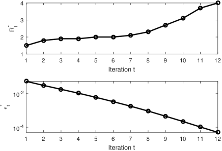
We run our DP scheme on a problem with relatively small desired EMSE, , in the last iteration . The signal is measured in an MP platform with processor nodes according to (2). The measurement rate is , and the noise variance is . The parameter (13). We use ECSQ [26, 25] as the quantizer in each processor node, and use the corresponding relation between the rate and distortion of ECSQ in our DP scheme. Note that we require the quantization bin size to be smaller than , according to Section II-B. Fig. 1 illustrates the optimal coding rate sequence and optimal EMSE given by DP as functions of the iteration number .
It is readily seen that after the first 5–6 iterations the coding rate seems near-linear. The next section proves that any optimal coding rate sequence is approximately linear in the limit of EMSE. However, our proof involves the large limit, and does not provide insights for small . We ran DP for various configurations. Examining all from our DP results, we notice that the coding rate is monotone non-decreasing, i.e., . This seems intuitive, because in early iterations of (MP-)AMP, the scalar channel noise is large, which does not require transmitting (cf. (8)) at high fidelity. Hence, a low rate suffices. As the iterations proceed, the scalar channel noise in (11) decreases, and the large quantization error would be unfavorable for the final MSE. Hence, higher rates are needed in later iterations.
IV Properties of Optimal Coding Rate Sequences
IV-A Intuition
We start this section by providing some brief intuitions about why optimal coding rate sequences are approximately linear when the EMSE is small.
Consider a case where we aim to reach a low EMSE. Montanari [6] provided a geometric interpretation of the relation between the MSE performance of AMP at iteration and the denoiser being used.444We will also provide such an interpretation in Section IV-B. In the limit of small EMSE, the EMSE decreases by a nearly-constant multiplicative factor per AMP iteration, yielding a geometric decay of the EMSE. In MP-AMP, in addition to the equivalent scalar channel noise , we have additive quantization error (11). In order for the EMSE in an MP-AMP system to decay geometrically, the distortion must decay at least as quickly. To obtain this geometric decay in , recall that in the high rate limit, the distortion-rate function typically takes the form [42] for some positive constant . We propose for to have the form, , where and are constants. In the remainder of this section, we first discuss the geometric interpretation of AMP state evolution, followed by our results about the linearity of optimal coding rate sequences. The detailed proofs appear in the appendices.

IV-B Geometric interpretation of AMP state evolution
Centralized SE: The equivalent scalar channel of AMP is given by (5). We re-write the centralized AMP SE (6) as follows [5, 7, 8],
| (19) |
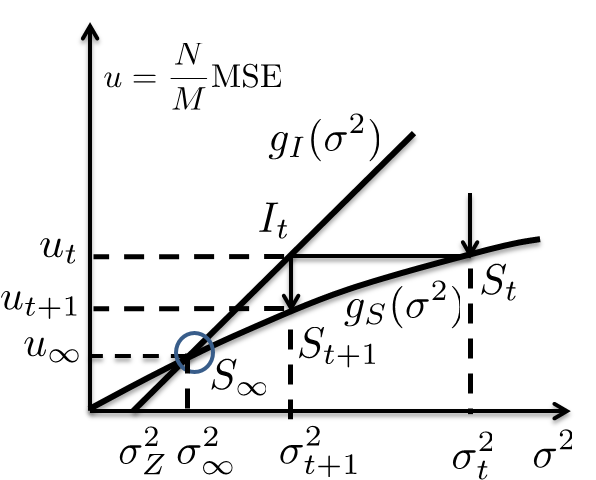
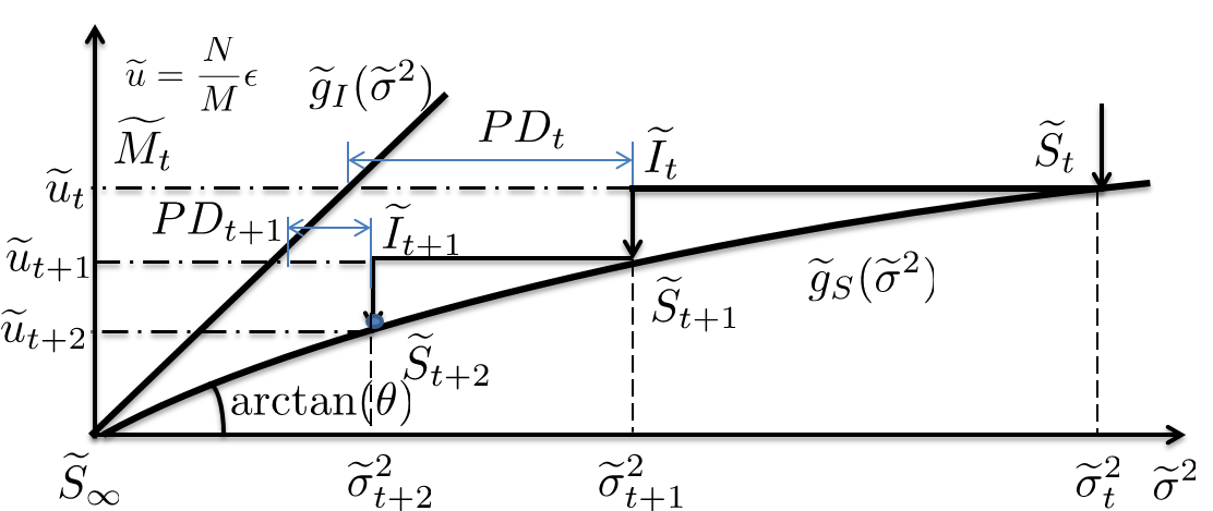
where denotes the MSE after denoising (5) using . The functions and are illustrated in Fig. 2 with solid curves; the meanings of and will become clear below. We see that is an affine function with unit slope, whereas is generally a nonlinear function of (see Fig. 2). The lines with arrows illustrate the state evolution (SE). Details appear below.
In Fig. 2, we present a geometric interpretation of SE. The horizontal axis is the scalar channel noise variance and the vertical axis represents the scaled MSE, . Let be the state point that is reached by SE in iteration . We follow the SE trajectory in Fig. 2, where represents the intermediate point in the transition between states and corresponding to iterations and , respectively. Observe that the points and have the same ordinate (), while and have the same abscissa (), which are related as and . As grows, converges to , which is the abscissa of the point . The ordinate of point is MSE∞, where . If we stop the algorithm at iteration , or equivalently at point , the corresponding MSE, MSET, has an EMSE of .
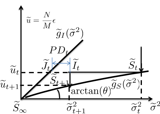
In Fig. 2, we zoom into the neighborhood of point . To make the presentation more concise, we vertically offset and by MMSE and horizontally offset them by ; we call the resulting functions and , respectively. Hence, the vertical axis in Fig. 2 represents the scaled EMSE, , and we have MMSE and MMSE. Observe that . Additionally, the slope of is , where is the first-order derivative of w.r.t. (Fig. 2). Because the MSE function for the MMSE-achieving denoiser is continuous and differentiable twice [43], we can invoke Taylor’s theorem to express
| (20) |
where and and are the first- and second-order derivatives of w.r.t. , respectively. Due to continuity and differentiability of the denoising function, is invertible in a neighborhood around , and its inverse is denoted by Invoking Taylor’s theorem,
| (21) |
where , and and are the first- and second-order derivatives of w.r.t. , respectively. When , and , and the higher-order terms become and . In other words, both and become approximately linear functions, as shown in Fig. 2. We further denote the slope of by , i.e.,
| (22) |
To calculate the slope , we first calculate the scalar channel noise variance for point , , by using replica analysis [14, 15],555The outcome of replica analysis [14, 15] is close to simulating SE (19) with a large number of iterations. and obtain . Moreover, the slope of satisfies ; otherwise, the curves and would not intersect at point .
Lossy SE: Considering lossy SE (12), we have
| (23) |
where is the number of processor nodes in an MP network, and is the expected distortion incurred by each node at iteration . Note that lossy SE has not been rigorously proved in the literature, although we argued in Section II-B that it tracks the evolution of the equivalent scalar channel noise variance when .
We notice the additional term , which corresponds to the distortion at the fusion center. Because the nodes transmit their signals with distortion , and their messages are independent, the fusion center’s signal has distortion . The lines with arrows in Fig. 2 illustrate the lossy SE after vertically offsetting and by MMSE and horizontally offsetting and by . After arriving at point , we move horizontally to , and obtain the ordinate of , , from . Geometrically, SE is dragged to the right by distance from point to , and then SE descends from to .
IV-C Asymptotic linearity of the optimal coding rate sequence
Recall from (20) that . Hence, as grows, (5) converges in distribution to . Therefore, the RD function converges to some fixed function as grows. For large coding rate , this function has the form
| (24) |
for some constant that does not depend on [42]. Note that the assumption of being small implicitly requires the coding rate used in the corresponding iteration to be large.
For an optimal coding rate sequence , we call the distortion , derived from (24), incurred by the optimal code rate at a certain iteration the optimal distortion. Correspondingly, we call the EMSE achieved by MP-AMP with , denoted by , the optimal EMSE at iteration . In the following, we state our main results on the optimal coding rate, the optimal distortion, and the optimal EMSE.
Theorem 1 (Linearity of the coding rate sequence)
Remark 1
Define the additive growth rate of an optimal coding rate sequence at iteration as . Theorem 1 not only shows that any optimal coding rate sequence grows approximately linearly in the low EMSE limit, but also provides a way to calculate its additive growth rate in the low EMSE limit. Hence, if the goal is to achieve a low EMSE, practitioners could simply use a coding rate sequence that has a fixed coding rate in the first few iterations and then increases linearly with additive growth rate .
The following theorem provides (i) the relation between the optimal distortion and the optimal EMSE in the large limit, and (ii) the convergence rate of the optimal EMSE .
Theorem 2
Assuming that lossy SE (23) holds, we have
| (27) |
Furthermore, the convergence rate of the optimal EMSE is
| (28) |
Theorem 2 is proved in Appendix -F. Note that meets the requirement discussed in Section II-B. Extending Theorems 1 and 2, we have the following result.
Corollary 3
Proof:
Remark 2
The key to the proofs of Theorems 1 and 2 is lossy SE (23). We expect that the linearity of the optimal coding rate sequence could be extended to other iterative distributed algorithms provided that (i) they have formulations similar to lossy SE (23) that track their estimation errors and (ii) their estimation errors converge geometrically. Moreover, formulations that track the estimation error in such algorithms might require less restrictive constraints than AMP. For example, consensus averaging [30, 31] only requires i.i.d. entries in the vector that each node in the network averages.
IV-D Comparison of DP results to Theorem 1
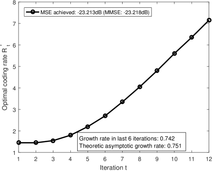
We run DP (cf. Section III) to find an optimal coding rate sequence for the setting of nodes, a Bernoulli Gaussian signal (18) with sparsity rate , measurement rate , noise variance , and parameter . The goal is to achieve a desired EMSE of 0.005 dB, i.e., . We use ECSQ [26, 25] as the quantizer in each processor node and use the corresponding relation between the rate and distortion of ECSQ in the DP scheme. Note that we require the quantization bin size to be smaller than , according to Section II-B. We know that ECSQ achieves a coding rate within an additive constant of the RD function [26]. Therefore, the additive growth rate of the optimal coding rate sequence obtained for ECSQ will be the same as the additive growth rate if the RD relation is modeled by [25, 24, 26, 35].
The resulting optimal coding rate sequence is plotted in Fig. 3. The additive growth rate of the last six iterations is , and the asymptotic additive growth rate according to Theorem 1 is . Note that we use in the discretized search space for . Hence, the discrepancy of 0.009 between the additive growth rate from the simulation and the asymptotic additive growth rate is within our numerical precision. In conclusion, our numerical result matches the theoretical prediction of Theorem 1.
V Achievable Performance Region
Following the discussion of Section II, we can see that the lossy compression of , can reduce communication costs. On the other hand, the greater the savings in the coding rate sequence , the worse the final MSE is expected to be. If a certain level of final MSE is desired despite a small coding rate budget, then more iterations will be needed. As mentioned above, there is a trade-off between , , and the final MSE, i.e., , and there is no solution that minimizes them simultaneously. To deal with such trade-offs, which implicitly correspond to sweeping in (13) in a multi-objective optimization (MOP) problem, it is customary to think about Pareto optimality [29].
V-A Properties of achievable region
For notational convenience, denote the set of all MSE values achieved by the pair for some parameter (13) by . Within , let the smallest MSE be . We now define the achievable set ,
where is the set of non-negative real numbers. That is, contains all tuples for which some instantiation of MP-AMP estimates the signal at the desired MSE level using iterations and aggregate coding rate .
Definition 3
The point is said to dominate another point , denoted by , if , , and . A point is Pareto optimal if there does not exist satisfying . Furthermore, let denote the set of all Pareto optimal points,
| (29) |
In words, the tuple is Pareto optimal if no other tuple exists such that , , and . Thus, the Pareto optimal tuples belong to the boundary of .
We extend the definition of the number of iterations to a probabilistic one. To do so, suppose that the number of iterations is drawn from a probability distribution over , such that . Of course, this definition contains a deterministic as a special case with and for all . Armed with this definition of Pareto optimality and the probabilistic definition of the number of iterations, we have the following lemma.
Lemma 2
For a fixed noise variance , measurement rate , and processor nodes in MP-AMP, the achievable set is a convex set.
Proof:
We need to show that for any , and any ,
| (30) |
This result is shown using time-sharing arguments (see Cover and Thomas [25]). Assume that , are achieved by probability distributions and , respectively. Let us select all parameters of the first tuple with probability and those of the second with probability . Hence, we have . Due to the linearity of expectation, and . Again, due to the linearity of expectation, , implying that (30) is satisfied, and the proof is complete. ∎
Definition 4
Let the function be the Pareto optimal rate function, which is implicitly described as . We further define implicit functions and in a similar way.
Corollary 4
The functions , , and are convex in their arguments.
Note that our proof for the convexity of the set might be extended to other iterative distributed learning algorithms that transmit lossily compressed messages.
V-B Pareto optimal points via DP
After proving that the achievable set is convex, we apply DP in Section III to find the Pareto optimal points, and validate the convexity of the achievable set.
According to Definition 3, the resulting tuple computed using DP (Section III) is Pareto optimal on the discretized search spaces. Hence, in this subsection, we run DP to obtain the Pareto optimal points for a certain distributed linear system by sweeping the parameter (13).
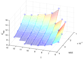
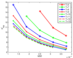
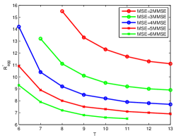
Consider the same setting as in Fig. 1, except that we analyze MP platforms [21, 22, 23] for different (13). Running the DP scheme of Section III, we obtain the optimal coding rate sequence that yields the lowest combined cost while providing a desired EMSE that is at most or equivalently . In Fig. 4, we draw the Pareto optimal surface obtained by our DP scheme, where the circles are Pareto optimal points. Fig. 4 plots the aggregate coding rate as a function of MSE for different optimal numbers of MP-AMP iterations . Finally, Fig. 4 plots the aggregate coding rate as a function of for different optimal MSEs. We can see that the surface comprised of the Pareto optimal points is indeed convex. Note that when running DP to generate Fig. 4, we used the RD function [25, 24, 26, 35] to model the relation between the rate and distortion at each iteration, which could be approached by VQ at sufficiently high rates. We also ignored the constraint on the quantization bin size (Section II-B). Therefore, we only present Fig. 4 for illustration purposes.
When a smaller MSE (or equivalently smaller EMSE) is desired, more iterations and greater aggregate coding rates (14) are needed. Optimal coding rate sequences increase to reduce when communication costs are low (examples are commercial cloud computing systems [23], multi-processor CPUs, and graphic processing units), whereas more iterations allow to reduce the coding rate when communication is costly (for example, in sensor networks [21, 22]). These applications are discussed in Section VI.
Discussion of corner points: We further discuss the corners of the Pareto optimal surface (Fig. 4) below.
-
1.
First, consider the corner points along the MSE coordinate.
-
•
If MSE MMSE (or equivalently ), then MP-AMP needs to run infinite iterations with infinite coding rates. Hence, and . The rate of growth of can be deduced from Theorem 1.
-
•
If MSE∗ (the variance of the signal (18)), then MP-AMP does not need to run any iterations at all. Instead, MP-AMP outputs an all-zero estimate. Therefore, and .
-
•
-
2.
Next, we discuss the corner points along the coordinate.
-
•
If , then the best MP-AMP can do is to output an all-zero estimate. Hence, and .
-
•
The other extreme, , occurs only when we want to achieve an MSE MMSE. Hence, .
-
•
-
3.
We conclude with corner points along the coordinate.
-
•
If , then the best MP-AMP can do is to output an all-zero estimate without running any iterations at all. Hence, and .
-
•
If , then the optimal scheme will use high rates in all iterations, and MP-AMP resembles centralized AMP. Therefore, the MSE∗ as a function of converges to that of centralized AMP SE (6).
-
•
VI Real-world Case Study
To showcase the difference between optimal coding rate sequences in different platforms, this section discusses several MP platforms including sensor networks [21, 22] and large-scale cloud servers [23]. The costs in these platforms are quite different due to the different constraints in these platforms, and we will see how they affect the optimal coding rate sequence . The changes in the optimal highlight the importance of optimizing for the correct costs.
VI-A Sensor networks
In sensor networks [21, 22], distributed sensors are typically dispatched to remote locations where they collect data and communicate with the fusion center. However, distributed sensors may have severe power consumption constraints. Therefore, low power chips such as the CC253X from Texas Instruments [44] are commonly used in distributed sensors. Some typical parameters for such low power chips are: central processing unit (CPU) clock frequency 32MHz, data transmission rate 250Kbps, voltage between 2V-3.6V, and transceiver current 25mA [44], where the CPU current resembles the transceiver current. Because these chips are generally designed to be low power, when transmitting and receiving data, the CPU helps the transceiver and cannot carry out computing tasks. Therefore, the power consumption can be viewed as constant. Hence, in order to minimize the power consumption, we minimize the total runtime when estimating a signal from MP-LS measurements (2) collected by the distributed sensors.
The runtime in each MP-AMP iteration (7)-(10) consists of (i) time for computing (7) and (8), (ii) time for encoding (8), and (iii) data transmission time for (9). As discussed in Section II-B, the fusion center may broadcast (10), and simple compression schemes can reduce the coding rate. Therefore, we consider the data reception time in the processor nodes to be constant. The overall computational complexity for (7) and (8) is . Suppose further that (i) each processor node needs to carry out two matrix-vector products in each iteration, (ii) the overhead of moving data in memory is assumed to be 10 times greater than the actual computation, and (iii) the clock frequency is 32MHz. Hence, we assume that the actual time needed for computing (7) and (8) is sec. Transmitting of length at coding rate requires sec, where the denominator is the data transmission rate of the transceiver. Assuming that the overhead in communication is approximately the same as the communication load caused by the actual messages, we obtain that the time requested for transmitting at coding rate is sec, where . Therefore, the total cost can be calculated from (13) with (13).
Because low power chips equipped in distributed sensors have limited memory (around 10KB, although sometimes external flash is allowed) [44], the signal length and number of measurements cannot be too large. We consider and spread over sensors, sparsity rate , and . We set the desired MSE to be dB above the MMSE, i.e., , and run DP as in Section III.666Throughout Section VI, we use the RD function [25, 24, 26, 35] to model the relation between rate and distortion at each iteration. We also ignore the constraint on the quantizer (Section II-B). Therefore, the optimal coding rate sequences in Section VI are only for illustration purposes. The coding rate sequence provided by DP is , , , , , , , , , , , , , , . In total we have MP-AMP iterations with bits aggregate coding rate (14). The final MSE () is , which is 0.5 dB from the MMSE () [14, 15, 12, 13].
VI-B Large-scale cloud server
Having discussed sensor networks [21, 22], we now discuss an application of DP (cf. Section III) to large-scale cloud servers. Consider the dollar cost for users of Amazon EC2 [23], a commercial cloud computing service. A typical cost for CPU time is /hour, and the data transmission cost is /GB. Assuming that the CPU clock frequency is 2.0GHz and considering various overheads, we need a runtime of sec and the computation cost is per MP-AMP iteration. Similar to Section VI-A, the communication cost for coding rate is . Note that the multiplicative factors of 20 in and 2 in are due to the same considerations as in Section VI-A, and the in is the number of bits per GB. Therefore, the total cost with MP-AMP iterations can still be modeled as in (13), where .
We consider a problem with the same signal and channel model as the setting of Section VI-A, while the size of the problem grows to and spread over computing nodes. Running DP, we obtain the coding rate sequence , , , , , , , , , , for a total of MP-AMP iterations with bits aggregate coding rate. The final MSE is , which is 0.49 dB above the MMSE. Note that this final MSE is 0.01 dB better than our goal of dB above the MMSE due to the discretized search spaces used in DP.
Settings with even cheaper communication costs: Compared to large-scale cloud servers, the relative cost of communication is even cheaper in multi-processor CPU and graphics processing unit (GPU) systems. We reduce by a factor of 100 compared to the large-scale cloud server case above. We rerun DP, and obtain the coding rate sequence , , , , , , , , , for and bits. Note that 10 iterations are needed for centralized AMP to converge in this setting. With the low-cost communication of this setting, DP yields a coding rate sequence within 0.5 dB of the MMSE with the same number of iterations as centralized AMP, while using an average coding rate of only 3.02 bits per iteration.
Remark 3
Let us review the cost tuples for our three cases. For sensor networks, ; for cloud servers, ; and for GPUs, . These cost tuples are different points in the Pareto optimal set (29). We can see for sensor networks that the optimal coding rate sequence reduces while adding iterations, because sensor networks have relatively expensive communications. The optimal coding rate sequences use higher rates in cloud servers and GPUs, because their communication costs are relatively lower. Indeed, different trade-offs between computation and communication lead to different aggregate coding rates and numbers of MP-AMP iterations . Moreover, the optimal coding rate sequences for sensor networks, cloud servers, and GPUs use average coding rates of , , and bits/entry/iteration, respectively. Compared to bits/entry/iteration single-precision floating point communication schemes, optimal coding rate sequences reduce the communication costs significantly.
VII Conclusion
This paper used lossy compression in multi-processor (MP) approximate message passing (AMP) for solving MP linear inverse problems. Dynamic programming (DP) was used to obtain the optimal coding rate sequence for MP-AMP that incurs the lowest combined cost of communication and computation while achieving a desired mean squared error (MSE). We posed the problem of finding the optimal coding rate sequence in the low excess MSE (EMSE=MSE-MMSE, where MMSE refers to the minimum MSE) limit as a convex optimization problem and proved that optimal coding rate sequences are approximately linear when the EMSE is small. Additionally, we obtained that the combined cost of computation and communication scales with . Furthermore, realizing that there is a trade-off among the communication cost, computation cost, and MSE, we formulated a multi-objective optimization problem (MOP) for these costs and studied the Pareto optimal points that exploit this trade-off. We proved that the achievable region of the MOP is convex.
We further emphasize that there is little work in the prior art discussing the optimization of communication schemes in iterative distributed algorithms. Although we focused on the MP-AMP algorithm, our conclusions such as the linearity of the optimal coding rate sequence and the convexity of the achievable set of communication/computation trade-offs could be extended to other iterative distributed algorithms including consensus averaging [30, 31].
Acknowledgments
The authors thank Puxiao Han and Ruixin Niu for numerous discussions about MP settings of linear systems and AMP. Mohsen Sardari and Mihail Sichitiu offered useful information about the practical distributed computing platforms of Section VI, and Cynthia Rush provided useful insights about the proof of AMP SE. The authors also thank Yanting Ma and Ryan Pilgrim for helpful comments about the manuscript.
-A Impact of the quantization error
This appendix provides numerical evidence that (i) the quantization error is independent of the scalar channel noise (11) in the fusion center and (ii) is independent of the signal . In the following, we simulate the AMP equivalent scalar channel in each processor node and in the fusion center. In the interest of simple implementation, we use scalar quantization (SQ) to quantize (8) (in each processor node) and hypothesis testing to evaluate (i) whether and (in the fusion center) are independent and (ii) whether and are independent. Both parts are necessary for lossy SE (12) to hold: part (i) ensures that we can predict the variance of by and part (ii) ensures that lossy MP-AMP falls within the general framework of Bayati and Montanari [7] and Rush and Venkataramanan [8], so that lossy SE (12) holds. Details about our simulation appear below.
Considering (5) and (8), we obtain that the AMP equivalent scalar channel in each processor node can be expressed as
| (31) |
where (5), and the variances of and can be expressed as and , respectively (12). Hence, we obtain . The signal follows (18) with . The entries of are i.i.d. and follow . Next, we apply an SQ to (31),
| (32) |
where denotes the quantization process, is the quantization error in processor node , and recall that the variance of is . We simulate the fusion center by calculating
| (33) |
where . Note that is Gaussian due to properties of AMP [5, 6, 7]. The total quantization error at the fusion center, , is also Gaussian, due to the central limit theorem. Hence, in order to test the independence of and (33), we need only test whether and are uncorrelated. We also test whether and are uncorrelated.
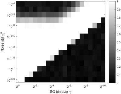
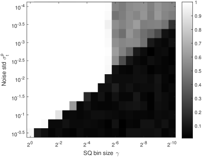
We study the settings and , where denotes the SQ bin size. In each setting, we simulate (31)–(33) 100 times and perform 100 Pearson correlation coefficient (PCC) tests [45] for and , respectively. The null hypothesis of the PCC tests [45] is that and are uncorrelated. The null hypothesis is rejected if the resulting -value is smaller than 0.05.
For each setting, we record the fraction of 100 tests where the null hypothesis is rejected, which is shown by the shades of gray in Fig. 5. The horizontal and vertical axes represent the quantization bin size and the standard deviation (std) , respectively. Similarly, we test and ; results appear in Fig. 5. We can see that when (bottom right corner), (i) and tend to be independent and (ii) and tend to be independent.
Now consider Fig. 5, which provides PCC test results evaluating possible correlations between and . There appears to be a phase transition that separates regions where and seem independent or dependent. We speculate that this phase transition is related to the pdf of . To explain our hypothesis, note that when the noise is low (top part of Fig. 5), the phase transition is less affected by noise, and the role of is smaller. By contrast, large noise (bottom) sharpens the phase transition.
In summary, it appears that when , we can regard (i) and to be independent and (ii) and to be independent. The requirement is motivated by Widrow and Kollár [41]; we leave the study of this phase transition for future work.
-B Numerical evidence for lossy SE
This appendix provides numerical evidence for lossy SE (23). We simulate two signal types, one is the Bernoulli Gaussian signal (18) and the other is a mixture Gaussian.
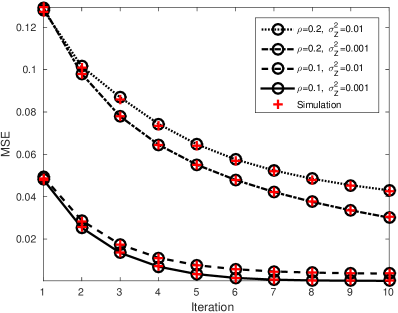
Bernoulli Gaussian signals: We generate 50 signals of length according to (18). These signals are measured by measurements spread over distributed nodes. We estimate each of these signals by running MP-AMP iterations. ECSQ is used to quantize (31), and (32) is encoded at coding rate . We simulate settings with sparsity rate and noise variance . In each setting, we randomly generate the coding rate sequence , s.t. the quantization bin size at each iteration satisfies (details in Appendix -A).777Note that the constraint on implies that is likely monotone non-decreasing. A Bayesian denoiser, , is used in (10). The resulting MSEs from the MP-AMP simulation averaged over the 50 signals, along with MSEs predicted by lossy SE (23), are plotted in Fig. 6. We can see that the simulated MSEs are close to the MSEs predicted by lossy SE.
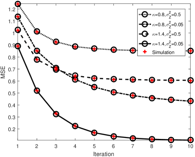
Mixture Gaussian signals: We independently generate 50 signals of length according to where follows a categorical distribution on alphabet , , , and . We simulate settings with , , , and . In each setting, we randomly generate the coding rate sequence , s.t. the quantization bin size at each iteration satisfies . The results are plotted in Fig. 6. The simulation results match well with the lossy SE predictions.
-C Integrity of discretized search space
When a coding rate is selected in MP-AMP iteration , DP calculates the equivalent scalar channel noise variance (11) for the next MP-AMP iteration according to (12). The variance is unlikely to lie on the discretized search space for , denoted by the grid . Therefore, in (17) does not reside in memory. Instead of brute-force calculation of , we estimate it by fitting a function to the closest neighbors of that lie on the grid and finding according to the fit function. We evaluate a linear interpolation scheme.
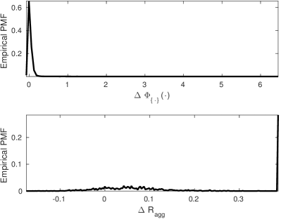
Interpolation in : We run DP over the original coarse grid with resolution dB, and a 4 finer grid with dB. We obtain the cost function with the coarse grid and the cost function with the fine grid . Next, we interpolate over the fine grid and obtain the interpolated . In order to compare with in a comprehensive way, we consider the settings given by the Cartesian product of the following variables: (i) the number of distributed nodes , (ii) sparsity rate , (iii) measurement rate , (iv) EMSE dB, (v) parameter , and (vi) noise variance . In total, there are 64 different settings. We calculate the error and plot the empirical probability mass function (PMF) of over all , , and all 64 settings. The resulting empirical PMF of is plotted in the top panel of Fig. 7. We see that with 99% probability, the error satisfies , which corresponds to an inaccuracy of approximately 0.2 in the aggregate coding rate .888Note that when calculating , we are still using the corresponding interpolation scheme. Although this comparison is not ideal, we believe it still provides the reader with enough insight. In the simulation, we used a resolution of . Hence, the inaccuracy of 0.2 in (over roughly 10 iterations) is negligible. Therefore, we use linear interpolation with a coarse grid with dB.
Integrity of choice of : We tentatively select resolution , and investigate the integrity of this over the 64 different settings above. After the coding rate sequence is obtained by DP for each setting, we randomly perturb by , where is the perturbed coding rate, the bias is , and is called the perturbed coding rate sequence. After randomly generating 100 different perturbed coding rate sequences , we calculate the aggregate coding rate (14), , of each ; we only consider the perturbed coding rate sequences that achieve EMSE no greater than the optimal coding rate sequence given by DP. The bottom panel of Fig. 7 plots the empirical PMF of , where and . Roughly 15% of cases in our simulation yield (meaning that the perturbed coding rate sequence has lower ), while for the other 85% cases, has lower . Considering the resolution , we can see that the perturbed sequences are only marginally better than . Hence, we verified the integrity of .
-D Proof of Lemma 1
Proof:
We show that our DP scheme (17) fits into Bertsekas’ formulation [27], which has been proved to be optimal. Under Bertsekas’ formulation, our decision variable is the coding rate and our state is the scalar channel noise variance . Our next-state function is the lossy SE (12) with the distortion being calculated from the RD function given the decision variable . Our additive cost associated with the dynamic system is . Our control law maps the state to a decision (the coding rate ). Therefore, our DP formulation (17) fits into the optimal DP formulation of Bertsekas [27]. Hence, our DP formulation (17) is also optimal for the discretized search spaces of and . ∎
-E Proof of Theorem 1
Proof:
Our proof is based on the assumption that lossy SE (12) holds. Consider the geometry of the SE incurred by for arbitrary iterations and , as shown in Fig. 8. Let and be the state and the optimal coding rate at iteration , respectively. We know that the slope of is . Hence, the length of line segment is . That is
| (34) |
Similarly, we obtain
| (35) |
where and obey
| (36) |
Recall that, according to Taylor’s theorem (21), we obtain that
| (37) |
with defined in (22). Although depends on , it is uniformly bounded, i.e., for some .
Fixing and , we explore different distortions and that obey (34)–(36). According to Definition 2, among distortions that obey (34)–(36), the optimal and correspond to the smallest aggregate rate at iterations and , . Considering (24), we have
Therefore, in the large limit, minimizing is identical to maximizing the product . Considering (34)–(36), our optimization problem becomes maximization over , where
| (38) |
Invoking Taylor’s theorem (37) and considering that , we solve the optimization problem (38) in two extremes: one with and the other with .
In the case of , we obtain
The maximum of is achieved when . That is,
| (39) |
Considering that , the root of the quadratic equation (39) is
| (40) |
where
| (41) |
We can further simplify (41) as
| (42) |
| (43) |
Plugging (43) into (34) and (35),
which leads to
| (44) |
These steps provided the optimal relation between and when . For the other extreme case, , similar steps will lead to (44), where the differences between the results are higher order terms. Note that for any the higher order term is bounded between the two extremes. Hence, the optimal and follow (44) leading to the first part of the claim (25). Considering (24) and (44),
Therefore, we obtain the second part of the claim (26). ∎
-F Proof of Theorem 2
Proof:
Our proof is based on the assumption that lossy SE (12) holds. Let us focus on an optimal coding rate sequence . Applying Taylor’s theorem to calculate the ordinate of point using its abscissa (Fig. 8), we obtain
| (45) |
Therefore,
| (46) |
Similarly, we obtain
| (47) |
Plugging (44) and (45) into (47), we obtain
| (48) |
On the other hand, . Therefore, considering (46) and (48), we obtain
which leads to . We obtain (27) by noting that the optimal EMSE at iteration t is . Plugging (27) into (46), we obtain (28). ∎
References
- [1] P. Han, J. Zhu, R. Niu, and D. Baron, “Multi-processor approximate message passing using lossy compression,” in Proc. IEEE Int. Conf. Acoustics, Speech, Signal Process. (ICASSP), Shanghai, China, Mar. 2016, pp. 6240–6244.
- [2] J. Zhu, A. Beirami, and D. Baron, “Performance trade-offs in multi-processor approximate message passing,” in Proc. IEEE Int. Symp. Inf. Theory (ISIT), Barcelona, Spain, July 2016, pp. 680–684.
- [3] D. Donoho, “Compressed sensing,” IEEE Trans. Inf. Theory, vol. 52, no. 4, pp. 1289–1306, Apr. 2006.
- [4] E. Candès, J. Romberg, and T. Tao, “Robust uncertainty principles: Exact signal reconstruction from highly incomplete frequency information,” IEEE Trans. Inf. Theory, vol. 52, no. 2, pp. 489–509, Feb. 2006.
- [5] D. L. Donoho, A. Maleki, and A. Montanari, “Message passing algorithms for compressed sensing,” Proc. Nat. Academy Sci., vol. 106, no. 45, pp. 18914–18919, Nov. 2009.
- [6] A. Montanari, “Graphical models concepts in compressed sensing,” Compressed Sensing: Theory and Applications, pp. 394–438, 2012.
- [7] M. Bayati and A. Montanari, “The dynamics of message passing on dense graphs, with applications to compressed sensing,” IEEE Trans. Inf. Theory, vol. 57, no. 2, pp. 764–785, Feb. 2011.
- [8] C. Rush and R. Venkataramanan, “Finite-sample analysis of approximate message passing,” Arxiv preprint arXiv:1606.01800, June 2016.
- [9] T. Tanaka, “A statistical-mechanics approach to large-system analysis of CDMA multiuser detectors,” IEEE Trans. Inf. Theory, vol. 48, no. 11, pp. 2888–2910, Nov. 2002.
- [10] D. Guo and S. Verdú, “Randomly spread CDMA: Asymptotics via statistical physics,” IEEE Trans. Inf. Theory, vol. 51, no. 6, pp. 1983–2010, June 2005.
- [11] D. Guo and C. C. Wang, “Multiuser detection of sparsely spread CDMA,” IEEE J. Sel. Areas Commun., vol. 26, no. 3, pp. 421–431, Apr. 2008.
- [12] D. Guo, D. Baron, and S. Shamai, “A single-letter characterization of optimal noisy compressed sensing,” in Proc. 47th Allerton Conf. Commun., Control, and Comput., Sept. 2009, pp. 52–59.
- [13] S. Rangan, A. K. Fletcher, and V. K. Goyal, “Asymptotic analysis of MAP estimation via the replica method and applications to compressed sensing,” IEEE Trans. Inf. Theory, vol. 58, no. 3, pp. 1902–1923, Mar. 2012.
- [14] J. Zhu and D. Baron, “Performance regions in compressed sensing from noisy measurements,” in Proc. IEEE Conf. Inf. Sci. Syst. (CISS), Baltimore, MD, Mar. 2013.
- [15] F. Krzakala, M. Mézard, F. Sausset, Y. Sun, and L. Zdeborová, “Probabilistic reconstruction in compressed sensing: Algorithms, phase diagrams, and threshold achieving matrices,” J. Stat. Mech. – Theory E., vol. 2012, no. 08, pp. P08009, Aug. 2012.
- [16] J. Mota, J. Xavier, and P. Aguiar, “Distributed basis pursuit,” IEEE Trans. Signal Process., vol. 60, no. 4, pp. 1942–1956, Apr. 2012.
- [17] S. Patterson, Y. C. Eldar, and I. Keidar, “Distributed compressed sensing for static and time-varying networks,” IEEE Trans. Signal Process., vol. 62, no. 19, pp. 4931–4946, Oct. 2014.
- [18] P. Han, R. Niu, M. Ren, and Y. C. Eldar, “Distributed approximate message passing for sparse signal recovery,” in Proc. IEEE Global Conf. Signal Inf. Process. (GlobalSIP), Atlanta, GA, Dec. 2014, pp. 497–501.
- [19] C. Ravazzi, S. M. Fosson, and E. Magli, “Distributed iterative thresholding for -regularized linear inverse problems,” IEEE Trans. Inf. Theory, vol. 61, no. 4, pp. 2081–2100, Apr. 2015.
- [20] P. Han, R. Niu, and Y. C. Eldar, “Communication-efficient distributed IHT,” in Proc. Signal Process. with Adaptive Sparse Structured Representations Workshop (SPARS), Cambridge, United Kingdom, July 2015.
- [21] G. J. Pottie and W. J. Kaiser, “Wireless integrated network sensors,” Commun. ACM, vol. 43, no. 5, pp. 51–58, May 2000.
- [22] D. Estrin, D. Culler, K. Pister, and G. Sukhatme, “Connecting the physical world with pervasive networks,” IEEE Pervasive Comput., vol. 1, no. 1, pp. 59–69, Jan. 2002.
- [23] “Amazon EC2,” https://aws.amazon.com/ec2/.
- [24] T. Berger, Rate Distortion Theory: Mathematical Basis for Data Compression, Prentice-Hall Englewood Cliffs, NJ, 1971.
- [25] T. M. Cover and J. A. Thomas, Elements of Information Theory, New York, NY, USA: Wiley-Interscience, 2006.
- [26] A. Gersho and R. M. Gray, Vector Quantization and Signal Compression, Kluwer, 1993.
- [27] D. P. Bertsekas, Dynamic Programming and Optimal Control, vol. 1, Athena Scientific Belmont, MA, 1995.
- [28] Y. Ma, D. Baron, and D. Needell, “Two-part reconstruction with noisy-sudocodes,” IEEE Trans. Signal Process., vol. 62, no. 23, pp. 6323–6334, Dec. 2014.
- [29] I. Das and J. E. Dennis, “Normal-boundary intersection: A new method for generating the Pareto surface in nonlinear multicriteria optimization problems,” SIAM J. Optimization, vol. 8, no. 3, pp. 631–657, Aug. 1998.
- [30] P. Frasca, R. Carli, F. Fagnani, and S. Zampieri, “Average consensus on networks with quantized communication,” Int. J. Robust Nonlinear Control, vol. 19, no. 16, pp. 1787–1816, Nov. 2008.
- [31] D. Thanou, E. Kokiopoulou, Y. Pu, and P. Frossard, “Distributed average consensus with quantization refinement,” IEEE Trans. Signal Process., vol. 61, no. 1, pp. 194–205, Jan. 2013.
- [32] J. Tan, D. Carmon, and D. Baron, “Signal estimation with additive error metrics in compressed sensing,” IEEE Trans. Inf. Theory, vol. 60, no. 1, pp. 150–158, Jan. 2014.
- [33] Y. Ma, J. Zhu, and D. Baron, “Approximate message passing algorithm with universal denoising and Gaussian mixture learning,” IEEE Trans. Signal Process., vol. 65, no. 21, pp. 5611–5622, Nov. 2016.
- [34] Y. Ma, D. Baron, and A. Beirami, “Mismatched estimation in large linear systems,” in Proc. IEEE Int. Symp. Inf. Theory (ISIT), July 2015, pp. 760–764.
- [35] C. Weidmann and M. Vetterli, “Rate distortion behavior of sparse sources,” IEEE Trans. Inf. Theory, vol. 58, no. 8, pp. 4969–4992, Aug. 2012.
- [36] S. Arimoto, “An algorithm for computing the capacity of an arbitrary discrete memoryless channel,” IEEE Trans. Inf. Theory, vol. 18, no. 1, pp. 14–20, Jan. 1972.
- [37] R. E. Blahut, “Computation of channel capacity and rate-distortion functions,” IEEE Trans. Inf. Theory, vol. 18, no. 4, pp. 460–473, July 1972.
- [38] K. Rose, “A mapping approach to rate-distortion computation and analysis,” IEEE Trans. Inf. Theory, vol. 40, no. 6, pp. 1939–1952, Nov. 1994.
- [39] Y. Linde, A. Buzo, and R. M. Gray, “An algorithm for vector quantizer design,” IEEE Trans. Commun., vol. 28, no. 1, pp. 84–95, Jan. 1980.
- [40] R. M. Gray, “Vector quantization,” IEEE ASSP Mag., vol. 1, no. 2, pp. 4–29, Apr. 1984.
- [41] B. Widrow and I. Kollár, Quantization Noise: Roundoff Error in Digital Computation, Signal Processing, Control, and Communications, Cambridge University press, 2008.
- [42] R. M. Gray and D. L. Neuhoff, “Quantization,” IEEE Trans. Inf. Theory, vol. IT-44, pp. 2325–2383, Oct. 1998.
- [43] Y. Wu and S. Verdú, “MMSE dimension,” IEEE Trans. Inf. Theory, vol. 57, no. 8, pp. 4857–4879, Aug. 2011.
- [44] Texas Instruments, A true system-on-chip solution for 2.4-GHz IEEE 802.15.4 and ZigBee applications, Apr. 2009, Rev. B.
-
[45]
“Pearson product-moment correlation coefficient,”
https://en.wikipedia.
org/wiki/Pearson_product-moment_correlation_coefficient.