Generation of a Supervised Classification Algorithm for Time-Series Variable Stars with an Application to the LINEAR Dataset

Abstract

With the advent of digital astronomy, new benefits and new problems have been presented to the modern day astronomer. While data can be captured in a more efficient and accurate manor using digital means, the efficiency of data retrieval has led to an overload of scientific data for processing and storage. This paper will focus on the construction and application of a supervised pattern classification algorithm for the identification of variable stars. Given the reduction of a survey of stars into a standard feature space, the problem of using prior patterns to identify new observed patterns can be reduced to time tested classification methodologies and algorithms. Such supervised methods, so called because the user trains the algorithms prior to application using patterns with known classes or labels, provide a means to probabilistically determine the estimated class type of new observations. This paper will demonstrate the construction and application of a supervised classification algorithm on variable star data. The classifier is applied to a set of 192,744 LINEAR data points. Of the original samples, 34,451 unique stars were classified with high confidence (high level of probability of being the true class).

1 Introduction

With the advent of digital astronomy, new benefits and new problems have been presented to the modern day astronomer. While data can be captured in a more efficient and accurate manor using digital means, the efficiency of data retrieval has led to an overload of scientific data for processing and storage. Where once the professional astronomer was faced with ten to a hundred data points for a given night, the now more common place “full-sky survey” mission results in millions of data points. This means that more stars, in more detail, are captured per night; but increasing data capture begets exponentially increasing data processing. No longer can the astronomer rely on manual processing, instead the profession as a whole has begun to adopt more advanced computational means. Database management, digital signal processing, automated image reduction, and statistical analysis of data have all made their way to the forefront of tools for the modern astronomer. Astro-statistics and astro-informatics are fields which focus on the application and development of these tools to help aid in the processing of large scale astronomical data resources.

This paper will focus on one facet of this budding area, the construction and application of a supervised pattern classification algorithm for the identification of variable stars. Given the reduction of a survey of stars into a standard feature space, the problem of using prior patterns to identify new observed patterns can be reduced to time tested classification methodologies and algorithms. Such supervised methods, so called because the user trains the algorithms prior to application using patterns with known (hence the supervised) classes or labels, provides a means to probabilistically determine the estimated class type of new observations. These methods have two large advantages over hand-classification procedures: the rate at which new data is processed is dependent only on the computational processing power available and the performance of a supervised classification algorithm is quantifiable and consistent. Thus the algorithm produces rapid, efficient, and consistent results.

This paper will be structured as follows. First, the data and feature space to be implemented for training will be reviewed. Second, we will discuss the class labels to be used and the meaning behind them. Third, a set of classifiers (multi-layer perceptron, random forest, k-nearest neighbor, and support vector machine) will be trained and tested on the extracted feature space. Fourth, performance statistics will be generated for each classifier and a comparing and contrasting of the methods will be discussed with a “champion” classification method being selected. Fifth, the champion classification method will be applied to the new observations to be classified. Sixth, an anomaly detection algorithm will be generated using the so called one-class support vector machine and will be applied to the new observations. Lastly, based on the anomaly detection algorithm and the supervised training algorithm a set of populations per class type will be generated. The result will be a highly reliable set of new populations per class type derived from the LINEAR survey.

1.1 Prior Work

The idea of constructing a supervised classification algorithm for stellar classification is not unique to this paper (see Dubath et al. 17 for a review), nor is the construction of a classifier for time variable stars. Methods pursued include the construction of a detector to determine variability (two-class classifier Barclay et al. 4), the design of random forests for the detection of photometric redshifts in spectra Carliles et al. [11], the detection of transient events Djorgovski et al. [16] and the development of machine-assisted discovery of astronomical parameter relationships Graham et al. [20]. Debosscher [14] explored several classification techniques for the supervised classification of variable stars, quantitatively comparing the performed in terms of computational speed and performance which they took to mean accuracy. Likewise, other efforts have focused on comparing speed and robustness of various methods (e.g. Blomme et al. 7, Pichara et al. 29, Pichara and Protopapas 28). These methods span both different classifiers and different spectral regimes, including IR surveys (Angeloni et al. 2 and Masci et al. 26), RF surveys [31], and optical [33].

2 Data

The procedure outlined in this paper will follow the standard philosophy for the generation of a supervised pattern classification algorithm as professed in Duda et al. [18]andHastie et al. [21], i.e. exploratory data analysis, training and testing of supervised classifier, comparison of classifiers in terms of performance, application of classifier. Our training data is derived from a set of three well known variable star surveys: the ASAS survey [30], the Hipparcos survey [27], and the OGLE dataset [38]. Data used for this study must meet a number of criteria:

1. Each star shall have differential photometric data in the u-g-r-i-z system

2. Each star shall have variability in the optical channel (band) that exceeds some fixed threshold with respect to the error in amplitude measurement

3. Each star shall have a consistent class label, should multiple surveys address the same star

2.1 Sample Representation

These requirements reduce the total training set down to 2054 datasets with 32 unique class labels. The features extracted are based on Fourier frequency domain coefficients[13], statistics associated with the time domain space, and differential photometric metrics; for more information see Richards et al. [33] for a table of all 68 features with descriptions. The 32 unique class labels can be further generalized into four main groups: eruptive, multi-star, pulsating, and “other” [14], the breakdown of characterizations for the star classes follows the following classifications:

• Pulsating

  • Giants: Mira, Semireg RV, Pop. II Cepheid, Multi. Mode Cepheid

  • RR Lyrae: FO, FM, and DM

  • “Others” : Delta Scuti, Lambda Bootis, Beta Cephei, Slowly Pulsating B, Gamma Doradus, SX Phe, Pulsating Be

• Erupting: Wolf-Rayet, Chemically Peculiar, Per. Var. SG, Herbig AE/BE, S Doradus, RCB and Classical T-Tauri

• Multi-Star: Ellipsoidal, Beta Persei, Beta Lyrae, W Ursae Maj.

• Other: Weak-Line T-Tauri, SARG B, SARG A, LSP, RS Cvn

The a priori distribution of stellar classes is given in 1 for the broad classes and in 2 for the unique classes:

Table 1: Broad Classification of Variable Types in the Training and Testing Dataset

Type	Count	% Dist
Multi-Star	514	0.25
Other	135	0.07
Pulsating	1179	0.57
Erupting	226	0.11

Table 2: Unique Classification of Variable Types in the Training and Testing Dataset

Class Type	% Dist	Class Type	% Dist
a. Mira	8.0%	m. Slowly Puls. B	1.5%
b1. Semireg PV	4.9%	n. Gamma Doradus	1.4%
b2. SARG A	0.7%	o. Pulsating Be	2.4%
b3. SARG B	1.4%	p. Per. Var. SG	2.7%
b4. LSP	2.6%	q. Chem. Peculiar	3.7%
c. RV Tauri	1.2%	r. Wolf-Rayet	2.0%
d. Classical Cepheid	9.9%	r1. RCB	0.6%
e. Pop. II Cepheid	1.3%	s1. Class. T Tauri	0.6%
f. Multi. Mode Cepheid	4.8%	s2. Weak-line T Tauri	1.0%
g. RR Lyrae FM	7.2%	s3. RS CVn	0.8%
h. RR Lyrae FO	1.9%	t. Herbig AE/BE	1.1%
i. RR Lyrae DM	2.9%	u. S Doradus	0.3%
j. Delta Scuti	6.5%	v. Ellipsoidal	0.6%
j1. SX Phe	0.3%	w. Beta Persei	8.7%
k. Lambda Bootis	0.6%	x. Beta Lyrae	9.8%
l. Beta Cephei	2.7%	y. W Ursae Maj.	5.9%

It has been shown [34] that how the classification of a multi-class problem is handled can affect the performance of the classifier; i.e. if the classifier is constructed to process all 32 unique classes as the same time, or if 32 different classifiers (detectors) are trained individually and the results are combined after application, or if a staged approach is best where a classifier is trained on the four “broad” classes first then a secondary classifier is trained on the unique class labels in each broad class [14]. The a priori distribution of classes, the number of features to use, and the number of samples in the training set are key factors in determining which classification procedure to use. This dependence is often best generalized as the “curse of dimensionality”[5], a set of problems that arise in machine learning that are tied to attempting to quantify a signature pattern for a given class, when the combination of a low number of training samples and high feature dimensionality results in a sparsity of data. Increasing sparsity results in a number of performance problems with the classifier, most of which amount to decrease generality (over-trained classifier) and decreased performance (low precision or high false alarm rate). Various procedures have been developed to address the curse of dimensionality, most often some form of dimensionality reduction technique is implemented or a general reframing of the classification problem is performed. For this effort, a reframing of the classification problem will be performed to address these issues

2.2 Feature Space

Prior to the generation of the supervised classification algorithm, an analysis of the training dataset is performed. This exploratory data analysis [37], is used here to understand the class separability prior to training, and to help the developer gain some insight into what should be expected in terms of performance of the final product. For example if during the course of the EDA it is found that the classes are linearly separable in the given dimensions using the training data, then we would expect a high performing classifier to be possible. Likewise, initial EDA can be useful in understanding the distribution of the classes in the given feature space answering questions like: are the class distributions multi-dimensional Gaussian? Do the class distributions have erratic shapes? Are they multi-modal? Not all classifiers are good for all situations, and often an initial qualitative EDA can help narrow down the window of which classifiers should be investigated and provide additional intuition to the analyst.

2.2.1 Exploratory Data Analysis

Principle Component Analysis (PCA) is one of many methods [18], and often the one most citied, when EDA of multi-dimensional data is being performed. Via orthogonal transformation, PCA rotates the feature space into a new representation where the feature dimensions are organized such that the first dimension (the principle component) has the largest possible variance, given the feature space. This version of PCA is the most simple and straight-forward; there are numerous variants, all of which attempt a similar maximization process (e.g., of variance, of correlation, of between group variance) but may also employ an additional transformation (e.g., manifold mapping, using the “kernel trick”, etc.). Using the broad categories defined for the variable star populations, PCA is performed in R using the FactoMineR package [23], and the first two components are plotted (see 1)

Figure 1: PCA applied to the ASAS+Hipp+OGLE dataset, with the broad class labels identified and the first two principle components plotted

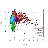
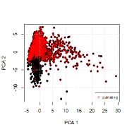
The PCA transformation is not enough to separate out the classes, however the graphical representation of the data does provide some additional insight about the feature space and the distribution of classes. The eruptive and multi-star populations appear to have a single mode in the dimensions presented in Figure 2, while the pulsating and the “other” categories appear to be much more irregular in shape. Further analysis addressing just the pulsating class shows that the distribution of stars with this label is spread across the whole of the feature space (2).

Figure 2: PCA applied to the ASAS+Hipp+OGLE dataset, only the stars classified as "pulsating" are highlighted

2.3 Effectiveness of Feature Space

In this representation of the feature space there is a significant overlap across all classes. Even if other methods of dimensionality reduction were implemented, for example supervised-PCA [3], linear separation of classes without dimensional transformation is not possible. Application of SPCA results in the Figure 4, which is also provided in movie form as digitally accessible media.

Figure 3: SPCA applied to the ASAS+Hipp+OGLE dataset

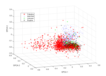
This non-Gaussian, non-linear separable class space requires further transformation to improve separation of classes or a classifier which performs said mapping into a space where the classes have improved separablity. Four classifiers are briefly discussed which address these needs.

3 Supervised Classification Development

All algorithms are implemented in the R language, version 3.1.2 (2014-10-31) – "Pumpkin Helmet", and operations are run on x86_64-w64-mingw32/x64 (64-bit) platform. Four classifiers are initially investigated: k-Nearest Neighbor (kNN), support vector machine (SVM), random forest (RF) and multi-layer perceptron (MLP).

The k-Nearest Neighbor algorithm implemented is based on the kNN algorithm outlined by Duda et al. [18] and Altman [1], with allowance for distance measurements using both $L_{1}$ (“taxi cab”) and $L_{2}$ (Euclidean distance) (see equation 1).

$\|x\|_{p}=(|x_{1}|^{p}+|x_{2}|^{p}+...+|x_{n}|^{n})^{1/p},p=1,2,...,\infty$

The testing set is implemented to determine both optimal distance method to be used and k value, i.e. number of nearest neighbors to count. A number of SVM packages exist [22], the e1071 package [15] is used in this study and was first implementation of SVM in R. It has been shown to perform well and contains a number of additional SVM utilities beyond the algorithm trainer that make it an ideal baseline SVM algorithm for performance testing. SVM decisions lines are hyperplanes, linear cuts that split the feature space into two sections; the optimal hyperplane is the one that has the larger distance to the nearest training data (i.e., maximum margin). Various implementations of the original algorithm exist, including the Kernel SVM [8] used here for this study with the Gaussian (or so called radial) Kernel. KSVM uses the so called “Kernel Trick” to project the original feature space into a higher dimension, resulting in hyperplane decision lines that are non-linear, a beneficial functionality should one find that the classes of interest are not linearly separable.

The multilayer perceptron supervised learning algorithm (MLP) falls into the family of neural network classifiers. The classifier can be simply described as layers (stages) of perceptron (nodes), where each perceptron performs a different transformation on the same dataset. These perceptrons often employ simple transformation (i.e., logit, sigmod, etc.), to go from the original input feature space, into a set of posterior probabilities (likelihoods per estimated class label). The construction of these layer and the transformations is beyond the scope of this article, and for more information on neural networks, back-propagation, error minimization and design of the classifier the reader is invited to review such texts as Rhumelhart et al. [32]. This study makes use of the R library “RSNNS,” for the construction and analysis of the MLP classifer used; see Bergmeir and Benítez [6]. Lastly, random forests are the conglomeration of sets of classification and regression trees (CARTs). The CART algorithm, made popular by Breiman et al. [10], generates decisions spaces by segmenting the feature space dimension by dimension. Given an initial training set, the original CART is trained such that each decision made maximally increases the purity of resulting two new populations. Each subsequent node following either similarly divides the received population into two new populations (with improved class purity) or is a terminal node, where no further splits are made and instead a class estimate is provided.

A detailed discussion of how the CART algorithm is trained, the various varieties of purity (or impurity) that can be used in the decision making process, and the pruning of a constructed tree given testing is beyond the scope of this article but are addressed in Breiman et al. as well as other standard pattern classification text (18, 21). Random Forests are the conglomeration of these CART classification algorithms, trained on variation of the same training set [9]. This ensemble classifier constructs a set of CART algorithms, each one trained on a reduction of the original training set (removal of some data points in the training set), this variation results in each CART algorithm in the set being slightly different. Given a new observed pattern applied to the set of CART classifiers, a set of decisions (estimated class labels) is generated. The Random Forest classifier combines these estimated class labels to generate a unified class estimate. This study makes use of the randomForest package in R, see Liaw and Wiener [25].

3.1 Training and Testing

The training of all four classifier types proceeds with roughly the same procedure; following the “one-vs.all” methodology for multi-class classification, a class type of interest is identified (either broad or unique), the original training set is split equally into a training set and a testing set with the a priori population distributions approximately equal to the population distribution of the combined training set. Adjustable parameters for each classifier are identified (RF: number of trees, kernel SVM: kernel spread, kNN: k value and p value, MLP: number of units in the hidden layers), and then the classifier is initially trained and tested against the testing population. Parameters are then adjusted (and subsequent classifiers are trained), and misclassification error is found as a function of the parameter adjustments. Those parameters resulting in a trained classifier with a minimal amount of error are implemented. For each classifier, two quantifications of performance are generated: a receiver operating curve (ROC) and a precision recall (PR) curve. Fawcett [19] outlines both, and discusses the common uses of each. Both concepts plot two performance statistics for a given classification algorithm, given some changing threshold value, which will for this study be a critical probability that the posterior probability of the class of interest (the target stellar variable) is compared against. These curves can be generated when the classifier is cast as a “two-class” problem, where one of the classes is the target (class of interest) while the other is not.

For any two-class classifier the metrics highlighted here can be generated and are a function of the decision space selected by the analyst. Frequently the acceptance threshold, i.e. the “hypothesized class” must have a posterior probability greater than some $\lambda$, is selected based on the errors of the classifier. Many generic classification algorithms are designed such that the false positive (fp) rate and 1 – true positive (tp) rate are both minimized. Often this practice is ideal; however the problem faced in the instances addressed in this article require additional considerations. We note two points:

1. When addressing the “unique” class types, there are a number of stellar variable populations which are relatively much smaller than others. This so called “class imbalance” has been shown [19] to cause problems with performance analysis if not handled correctly. Some classification algorithms adjust for this imbalance, but often additional considerations must be made, specifically when reporting performance metrics.

2. Minimization of both errors, or minimum-error-rate classification, is often based on the zero-one loss function. In this case, it is assumed that the cost of a false positive (said it was, when it really was not) is the same as a false negative (said it wasn’t, when it really was). If the goal of this study is to produce a classifier that is able to classify new stars from very large surveys, some of which are millions of stars big, the cost of returning a large number of false alarms is much higher than the cost of missing some stars in some classes. Especially when class separation is small (if not non-existent), if the application of the classifier results in significant false alarms the inundation of an analyst with bad decisions will likely result in a general distrust of the classifier algorithm.

The ROC curve expresses the adjustment of the errors as a function of the decision criterion. Likewise, the PR curve expresses the adjustment of precision (the percentage of true positives out of all decisions made) and recall (true positive rate) as a function of the decision criterion. By sliding along the ROC or PR curve, we can change the performance of the classifier. Note that increasing the true positive rate causes an increase in the false positive rate as well (and vice versa). Often a common practice is to fix [35] one of the metrics, false positive rate, of all classifiers used. For example, minimum requirements might be a false positive rate of 5%, if the ROC curve was resulting from a classifier designed; we would expect a 20% true positive rate.

Similar to the ROC curve, the PR curve demonstrates how performance varies between precision and recall for a given value of the threshold. It is apparent that the PR and ROC curves are related [12], both have true-positive rate as an axis (TP Rate and Recall are equivalent), both are functions of the threshold used in the determination of estimated class for a new patter (discrimination), both are based on the confusion matrix and the associated performance metrics. Thus fixing the false alarm rate, not only fixes the true positive rate but also the precision of the classifier. If the interest was a general comparison of classifiers, instead of selecting a specific performance level, Fawcett [19] suggests that the computation of Area-Under-the-Curve quantifies either the PR and ROC curve into a single “performance” estimate that represents the classifier as a whole. The ROC-AUC of a classifier is equivalent to the probability that the classifier will rank a randomly chosen positive instance higher than a randomly chosen negative instance. The PR-AUC of a classifier is roughly the mean precision of the classifier. Both ROC and PR curves should be considered when evaluating a classifier [12], especially when class imbalances exist. For this study, the best performing classifier will be the one that maximizes both the ROC-AUC and the PR-AUC. Likewise, when the final performance of the classifier is proposed, false positive rate and precision will be reported and used to make assumption about the decisions made by the classification algorithm.

3.2 Performance Analysis - Supervised Classification

Based on the foundation of performance analysis methods, ROC and PR curves, and AUC discussed, the study analyzes classification algorithms applied to both the broad and unique (individual) class labels.

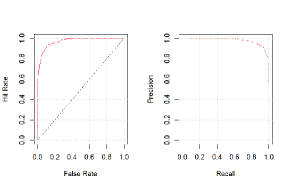
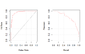
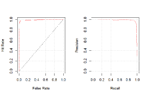
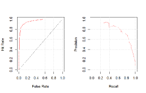
3.2.1 Broad Classes - Random Forest

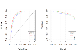
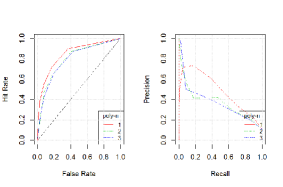
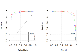
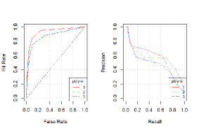
Initially an attempt was made to adjust both the number of trees (ntree) and the number of variables randomly sampled as candidates at each split (mtry). It was found that for the training datasets, that neither resulted in a major difference in performance when adjusted. Based on Breiman et al. [10] recommendation, mtry was set to $\sqrt{M}$, where $M$ is the number of features. The parameters ntree was set to 100, based on the work performed by Debosscher [14]. Classifiers were then generated based on the training sample, and the testing set was used to generate the ROC and PR AUC for each one-vs-all classifier. The associated curves are given in Appendix A, the resulting AUC estimates are in 3:

Table 3: ROC/PR AUC Estimates based on training and testing for the Random Forest Classifier.

AUC	Pulsating	Eruptive	Multi-Star	Other
ROC	0.971	0.959	0.992	0.961
PR	0.979	0.788	0.986	0.800

3.2.2 Broad Classes - Kernel SVM

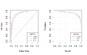
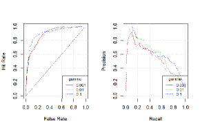
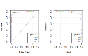
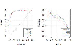
Instead of using the “hard” class estimates, common with SVM usage, the “soft” estimates i.e. posterior probabilities are used. This allows for the thresholding necessary to construct the PR and ROC curves. Kernel spreads of 0.001, 0.01, and 0.1 were tested (set as the variable gamma in R), the associated PR and ROC curve are given in Appendix A. It was found that 0.1 was optimal for the feature space (using Gaussian Kernels). The associated curves are given in Appendix A, the resulting AUC estimates are in 4:

Table 4: ROC/PR AUC Estimates based on training and testing for the Kernel SVM Classifier.

AUC	Pulsating	Eruptive	Multi-Star	Other
ROC	0.938	0.903	0.979	0.954
PR	0.952	0.617	0.968	0.694

3.2.3 Broad Classes - k-NN

It was found, that for the training set used, that increasing performance was gained with increasing values of k (number of nearest neighbors). Gains in performance were limiting after k = 4, and a value of k = 10 was selected to train with. The value of the polynomial defined in the generation of distance (via $L^{p}$-norm) was varied between 1 and 3, with decreasing performance found for p > 3. The associated PR and ROC curves were generated for values of p < 4. The associated curves are given in Appendix A, the resulting AUC estimates for p < 3 are in 5:

Table 5: ROC/PR AUC Estimates based on training and testing for the k-NN Classifier.

	AUC	Pulsating	Eruptive	Multi-Star	Other
p-1	ROC	0.919	0.847	0.980	0.928
	PR	0.931	0.480	0.959	0.597
p-2	ROC	0.901	0.802	0.967	0.877
	PR	0.918	0.368	0.931	0.519

3.2.4 Broad Classes - MLP

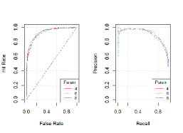
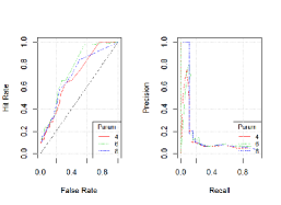
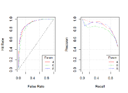
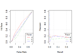
There are two variables associated with MLP algorithm training: the number of units in the hidden layers (size) and the number of parameters for the learning function to use (learnParam). It was found that for the dataset: The learnParam function had little effect on the performance of the classifier, and it was taken to be 0.1 for implementation here. The variable size did have an effect, an initial study of values between 4 and 18 demonstrated that the best performance occurred between 4 and 8. PR and ROC curves for these values were generated and are in Appendix A, the resulting AUC estimates for values 4,6 and 8 are in 6:

Table 6: ROC/PR AUC Estimates based on training and testing for the MLP Classifier.

	AUC	Pulsating	Eruptive	Multi-Star	Other
	ROC	0.928	0.694	0.914	0.585
	PR	0.916	0.120	0.869	0.183
	ROC	0.933	0.751	0.888	0.473
	PR	0.909	0.139	0.797	0.123
	ROC	0.920	0.706	0.914	0.529
	PR	0.903	0.175	0.854	0.159

3.2.5 Unique Classes

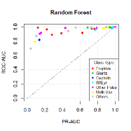
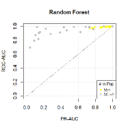
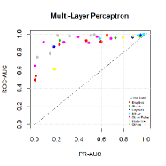
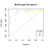
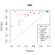
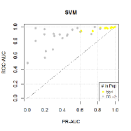
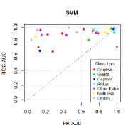
Analysis of the broad classes provided insight into the potential of a staged classifier. The performance of the broad classification algorithms does not suggest that the supervised variable star classification problem would be benefited by a staged design. The RF classifier performed best across all broad classes and against all other classifiers, but still had significant error; had the broad classes perfectly separated further analysis into the staged design would have been warranted. Instead, two-class classifier designed based on the unique classes are explored. Similar to the broad classification methodology, the training sample is separated into a training set and a testing data set for each unique class type for training in a two-class classifier. Again, the testing data is used to minimize the misclassification error, and find optimal parameters for each of the classifiers. Each classifier is then optimal for the particular class of interest. With the change of design, a change of performance analysis is also necessary. With nearly ten times the number of classes, a comparison of ROC and PR curves per classifier type and per class type requires a methodology that allows the information plotted on a single plot (direct comparison). Keeping with the discussion outlined by Davis and Goadrich [12], we plot ROC vs. PR for each classifier (4as an example).

Figure 4: ROC vs. PR AUC Plot for Multi-Layer Perceptron Classifier, generic class types (Eruptive, Giants, Cephids, RRlyr, Other Pulsing, Multi-star, and “other”) are colored. The line y = x is plotted for reference (dashed line)

The set of these performance analysis graphs are in Appendix B. A comparison of the general performance of each classifier can be derived from the generation of AUC for each of the performance curves. Here, the quantification of general performance for a classifier is given as either mean precision across all class types or via non-parametric analysis of the AUC. The non-parametric analysis used is compiled as follows: for each class of stars, the average performance across classifiers is found, if for a classifier the performance is greater than the mean, an assignment of +1 is given, else -1. Over all classes, the summation of assignments is taken and given in 7.

Table 7: Performance Analysis of Individual Classifiers

	ROC-AUC		PR-AUC
	Mean	Non-Para.	Mean	Non-Para.
KNN-Poly-1	0.884	2	0.530	8
SVM	0.905	-4	0.407	-26
MLP	0.894	2	0.470	-8
RF	0.948	22	0.595	14

It is apparent that the RF classifier out-performs the other three classification algorithms, using both the mean of precision as well as a non-parametric comparison of the AUC statistics. The plot comparing ROC-AUC and PR-AUC for the Random Forest classifier is presented in 5.

Figure 5: Random Forest, Individual Classification, Performance Analysis

(a)

(b)

Based on 5, it is observed that star populations of similar class types do not necessarily cluster together. Additionally it is apparent that the original size of the population in the training set, while having some effect on the ROC-AUC, has a major effect on the resulting PR-AUC. Figure 11.b demonstrates that for those classes with an initial population of 55 (empirically guessed value), that the precision is expected to be greater than 70%. Surprisingly though for classes with an initial population of 55 or less, the limits of precision are less predictable and in fact appear to be random with respect to class of interest training size. Thus, without further training data or feature space improvements, the performance statistics graphed in 5 are the statistics that will be used as part of the application of the classifier to the LINEAR dataset.

3.3 Performance Analysis - Anomaly Detection

In addition to the pattern classification algorithm outlined, the procedure outlined here includes the construction of a One-Class Support Vector Machine (OC-SVN) for use as an anomaly detector. The pattern classification algorithms presented and compared as part of this analysis, partition the entire decision space. For the random forest, kNN, MLP and SVM two-class classifier algorithms, there is no consideration for deviations of patterns beyond the training set observed, i.e. absolute distance from population centers. All of the algorithms investigated consider relative distances, i.e. is the new pattern P closer to the class center of B or A? Thus, despite that an anomalous pattern is observed by a new survey, the classifier will attempt to estimate a label for the observed star based on the labels it knows. To address this concern, a one-class support vector machine is implemented as an anomaly detection algorithm. Lee and Scott (2007) describe the design and construction of such an algorithm. Similar to the Kernel-SVM discussed prior, the original dimensionality is expanded using the Kernel trick (Gaussian Kernels) allowing complex regions to be more accurately modeled. For the OC-SVM, the training data labels are adjusted such that all entered data is of class type one (+1). A single input pattern at the origin point is artificially set as class type two (-1). The result is the “lassoing” or dynamic encompassing of “known” data patterns. The lasso boundary represents the division between known (previously observed) regions of feature space and unknown (not-previously observed) regions. New patterns observed with feature vectors occurring in this unknown region are considered anomalies or patterns without support, and the estimated labels returned from the supervised classification algorithms should be questioned, despite the associated posterior probability of the label estimate [36]. The construction of the OC-SVM to be applied as part of this analysis starts with the generation of two datasets (training and testing) from the ASAS + Hipp + OGLE training data. The initial training set is provided to the OC-SVM [24] algorithm which generates the decision space (lasso). This decision space is tested against the training data set; and the fraction of points declared to be anomalous is plotted against the spread of the Kernel used in the OC-SVM (6).

Figure 6: Fraction of Anomalous Points Found in the Training Dataset as a Function of the Gaussian Kernel Spread Used in the Kernel-SVM

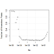
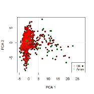
Because of the hyper-dimensionality, the OC-SVM algorithm is unable to perfectly encapsulate the training data; however a minimization can be found and estimated. The first two principle components of the training data feature space are plotted for visual inspection (7), highlighting those points that were called “anomalous” based on a nu value (kernel spread) of 0.001. Less than 5% of the points are referred to as anomalies (~falsely).

Figure 7: Plot of OC-SVM Results Applied to Training Data Only

Further testing is performed on the anomaly space, using the second dataset generated. As both datasets originate from the same parent population, the OC-SVM algorithm parameter (nu) is tuned to a value that maximally accepts the testing points (8).

Figure 8: OC-SVM testing of the Testing data

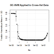
The minimum fraction was found at a nu of 0.03. The OC-SVM was applied to the LINEAR dataset with the optimal kernel spread. All 192,744 datasets were processed, with 58,312 (False, or “anomalous”) and 134,432 (True, or “expected”) decision made, i.e. ~30% of the LINEAR dataset is considered anomalous based on the ASAS+HIPP+OGLE training dataset feature space.

4 Application of Supervised Classifer to LINEAR Dataset

4.1 Analysis and Results

For application to the LINEAR dataset, a RF classifier is constructed based on the training set discussed prior. The classifiers are designed using the one-vs.-all methodology, i.e. each stellar class has its own detector (i.e. overlap in estimated class labels is possible), therefore 32 individual two-class classifiers (detectors) are generated. The individual classification method (one-vs.-all) allows for each given star to have multiple estimated labels (e.g. multiple detectors returning a positive result for the same observation). The one-vs.-all methodology also allows the training step of the classification to be more sensitive to stars who might have been under-represented in the training sample, improving the performance of the detector overall. Based on the testing performance results (ROC and PR curves) presented for the individual classifiers, the critical statistic used for the RF decision process was tuned such that a 0.5% false positive rate is expected when applied to the LINEAR dataset. In addition to the RF classifier, an OC-SVM anomaly detection algorithm was trained, an used to determine if samples from the LINEAR dataset are anomalous with respect to the ASAS+OGLE+HIPP dataset. Applying the RF classifier(s) and the OC-SVM algorithm to the LINEAR dataset the following was found using a threshold setting corresponding to a false alarm rate of 0.5% (see ROC curve analysis). Given an initial set of LINEAR data (192,744 samples), the following table was constructed based on the results of the application of the isolated one-vs.-all RF classifiers only:

Table 8: Initial results from the application of the RF classifier(s)

Class Type	Est. Pop	Class Type	Est. Pop
a. Mira	3256	m. Slowly Puls. B	2
b1. Semireg PV	7	n. Gamma Doradus	2268
b2. SARG A	4291	o. Pulsating Be	14746
b3. SARG B	30	p. Per. Var. SG	284
b4. LSP	10	q. Chem. Peculiar	10
c. RV Tauri	5642	r. Wolf-Rayet	3970
d. Classical Cepheid	31	r1. RCB	1253
e. Pop. II Cepheid	326	s1. Class. T Tauri	17505
f. Multi. Mode Cepheid	556	s2. Weak-line T Tauri	4945
g. RR Lyrae FM	13470	s3. RS CVn	40512
h. RR Lyrae FO	1276	t. Herbig AE/BE	1358
i. RR Lyrae DM	9800	u. S Doradus	2185
j. Delta Scuti	493	v. Ellipsoidal	132
j1. SX Phe	9118	w. Beta Persei	481
k. Lambda Bootis	69	x. Beta Lyrae	2
l. Beta Cephei	2378	y. W Ursae Maj.	1365

103628 stars were not classified (~54%) and of those 11619 were considered “Anomalous”. 57848 stars were classified only once (30%) and of those 23397 were considered “Anomalous”. 31268 stars were classified with multiple labels (~16%) and of those 23296 were considered “Anomalous”. The set of stars that were both classified once and did not have anomalous patterns (34,451), are broken down by class type in 9.

Table 9: Initial results from the application of the RF classifier(s) and the OC-SVM anomaly detection algorithm, classes that are major returned classes (>1% of the total return set) are in bold

Class Type	Est. Pop	% Total	Class Type	Est. Pop	% Total
a. Mira	15	0.04%	m. Slowly Puls. B	2	0.002%
b1. Semireg PV	1	0.002%	n. Gamma Doradus	2268	3.8%
b2. SARG A	1362	4.0%	o. Pulsating Be	14746	0.61%
b3. SARG B	0	0%	p. Per. Var. SG	284	0.26%
b4. LSP	1	0.002%	q. Chem. Peculiar	10	0%
c. RV Tauri	538	1.6%	r. Wolf-Rayet	3970	6.2%
d. Classical Cepheid	2	0.006%	r1. RCB	1253	0.01%
e. Pop. II Cepheid	50	0.15%	s1. Class. T Tauri	17505	5.4%
f. Multi. Mode Cepheid	286	0.83%	s2. Weak-line T Tauri	4945	3.3%
g. RR Lyrae FM	2794	8.1%	s3. RS CVn	40512	46.6%
h. RR Lyrae FO	710	2.1%	t. Herbig AE/BE	1358	0.33%
i. RR Lyrae DM	2350	6.8%	u. S Doradus	2185	1.7%
j. Delta Scuti	8	0.02%	v. Ellipsoidal	132	0.08%
j1. SX Phe	1624	4.7%	w. Beta Persei	481	0.42%
k. Lambda Bootis	1	0.002%	x. Beta Lyrae	2	0.006%
l. Beta Cephei	25	0.07%	y. W Ursae Maj.	1365	3.1%

The listing of individual discovered populations are provided digitally via request (to the author). Two classes were not detected confidently out of the LINEAR dataset: SARG B and Chemically Peculiar. This does not mean that these stars are not contained in the LINEAR dataset. Similarly, those stars that were not classified are not necessarily in a “new” class of stars. There are a number of possibilities why these stars were not found in the survey including:

1. Poor separation between the class of interest (for a given detector) and other stars. Poor separation could result in either the posterior probability not being high enough to detect the star, or more likely the star being classified as two different types at the same time

2. Poor initial quantification of the signature class pattern in the training set feature space. If the training sample representing a given class type spanned only a segment of the signature class pattern region, the potential for an under-sampled or poorly bounding feature space exists. Furthermore, application of the anomaly detection algorithm, or any of the pattern classification algorithms, would result in decision-lines lassoing the under-sampled feature space, cutting through the “true class pattern region”. New observations of that class type, if they occurred outside of the original under-sampled space, would likely be flagged by the anomaly detection algorithm or as a different class.

Thus, those stars positively classified by the set of detectors used represent the set of LINEAR observations that have patterns that are consistent with those observed in the training set. As part of the testing process we estimate both a false alarm rate (FAR) of 0.5% across all classes and a precision rate from the PR curve. Then, each one-vs.-all detector will have a different precision rate, since the FAR is fixed. The precision rate estimates based on testing are given in 10. An adjusted estimate of “true” returned population sizes can be estimated by considering the precision rate, i.e., if 15 Mira stars were detected, and the Mira detector had a precision of ~94% percent, then potentially 1 of those detections is a false positive.

Table 10: Precision Rate Estimates Per Class Type (in fractions), Bolded Classes are those with Precisions < 80%

Class Type	Precision	Class Type	Precision
a. Mira	0.94	m. Slowly Puls. B	0.91
b1. Semireg PV	0.97	n. Gamma Doradus	0.88
b2. SARG A	0.76	o. Pulsating Be	0.91
b3. SARG B	0.94	p. Per. Var. SG	0.94
b4. LSP	0.91	q. Chem. Peculiar	0.94
c. RV Tauri	0.86	r. Wolf-Rayet	0.91
d. Classical Cepheid	0.94	r1. RCB	0.73
e. Pop. II Cepheid	0.87	s1. Class. T Tauri	0.75
f. Multi. Mode Cepheid	0.87	s2. Weak-line T Tauri	0.75
g. RR Lyrae FM	0.91	s3. RS CVn	0.74
h. RR Lyrae FO	0.88	t. Herbig AE/BE	0.86
i. RR Lyrae DM	0.73	u. S Doradus	0.67
j. Delta Scuti	0.95	v. Ellipsoidal	0.78
j1. SX Phe	0.73	w. Beta Persei	0.97
k. Lambda Bootis	0.91	x. Beta Lyrae	0.97
l. Beta Cephei	0.91	y. W Ursae Maj.	0.91

Table 11: True Recovery Estimates based on Precision Estimates and the Number of Stars Detected by the RF classifier

Class Type	Est. Pop	Class Type	Est. Pop
a. Mira	14	m. Slowly Puls. B	0
b1. Semireg PV	0	n. Gamma Doradus	1159
b2. SARG A	1035	o. Pulsating Be	192
b3. SARG B	0	p. Per. Var. SG	85
b4. LSP	0	q. Chem. Peculiar	0
c. RV Tauri	462	r. Wolf-Rayet	1939
d. Classical Cepheid	1	r1. RCB	2
e. Pop. II Cepheid	43	s1. Class. T Tauri	1383
f. Multi. Mode Cepheid	248	s2. Weak-line T Tauri	843
g. RR Lyrae FM	2542	s3. RS CVn	11850
h. RR Lyrae FO	624	t. Herbig AE/BE	96
i. RR Lyrae DM	1715	u. S Doradus	387
j. Delta Scuti	7	v. Ellipsoidal	21
j1. SX Phe	1185	w. Beta Persei	138
k. Lambda Bootis	0	x. Beta Lyrae	1
l. Beta Cephei	22	y. W Ursae Maj.	986

5 Conclusions

With the onset of large scale stellar surveys, methods such as the supervised classifier are becoming more and more necessary. The volume of data returned by these surveys has exceeded the amount that can be hand processed in any reasonable amount of time. Data science, statistics, digital signal processing, and other exploratory data analysis methods are then necessary to produce at a minimum the actionable information demonstrated in this paper. This paper outlines the application of one of these tools, supervised classification algorithms, to be used in the identification of stellar variables. Variable stars provide an opportunity to observe not only differential photometric features, but also single (or multi-band) time-domain feature, providing a large feature space with which stellar classes can be separated. Time domain features can include descriptive statistics associated with the time domain variability, or the transformation of the time domain feature into a basis representation that is constant over the life-time of observations of the star. Accurate handling of these features can provide separablity in classes, allowing machine operations to rapidly categorize new observations.

This paper has demonstrated the construction and application of a supervised classification algorithm on variable star data. Such an algorithm, will process observed stellar features and produce quantitative estimates of stellar class label. Using a hand-process (verified) dataset derived from the ASAS, OGLE, and Hipparcos survey, an initial training and testing set was derived. The trained one-vs.-all algorithms were optimized using the testing data via minimization of the misclassification rate. From application of the trained algorithm to the testing data, performance estimates can be quantified for each one-vs.-all algorithm. The Random Forest supervised classification algorithm was found to be superior for the feature space and class space operated in. Similarly, a one-class support vector machine was trained in a similar manor, and designed as an anomaly detector.

With the classifier and anomaly detection algorithm constructed, both were applied to a set of 192744 LINEAR data points. Of the original samples, Setting the threshold of the RF classifier using a false alarm rate of 0.5%, 34,451 unique stars were classified only once in the one-vs.-all scheme and were not identified by the anomaly detection algorithm. The total population is partitioned into the individual stellar variable classes; each subset of LINEAR ID corresponding to the matched patterns is stored in a separate file and accessible to the reader. While less than 18% of the LINEAR data was classified, the class labels estimated have a high level of probability of being the true class based on the performance statistics generated for the classifier, and the threshold applied to the classification process.

Further improvement in both the initial training dataset is necessary, if the requirements of the supervised classification algorithm are to be met (100% classification of new data). Larger training data, with more representation (support) is needed to improve the class space representation used by the classifier, and reduce the size of the “anomalous” decision region. Specifically, additional example of the under-sampled variable stars, enough to perform k-fold cross-validation would yield improved performance and increased generality of the classifier. An improved feature space could also benefit the process, if new features were found to provide additional linear separation for certain classes. However, additional dimensionality without reduction of superfluous features is warned against as it may only worsen the performance issues of the classifier. Instead, investigation into the points found to be anomalous in under-sampled classes, and determination if they are indeed of the class reported by the classifier designed here would be of benefit, as this points would serve to not only bolster the number of training points used in the algorithm, but they would also increase the size (and support) of the individual class spaces. Implementation of these concepts, with a mindfulness of the changing performance of the supervised classification algorithm, could result in performance improvements across the class space.

Appendix A Broad Class Performance Results

Figure 9: Random Forest, mtry = 8, ntree = 100, (a) Pulsating, (b) Erupting, (c) Multi-Star, (d) Other

(a)	(b)
(c)	(d)

Figure 10: SVM, (a) Pulsating, (b) Erupting, (c) Multi-Star, (d) Other

(a)	(b)
(c)	(d)

Figure 11: kNN, (a) Pulsating, (b) Erupting, (c) Multi-Star, (d) Other

(a)	(b)
(c)	(d)

Figure 12: MLP, (a) Pulsating, (b) Erupting, (c) Multi-Star, (d) Other

(a)	(b)
(c)	(d)

Figure 13: MLP, Individual Classification, Performance Analysis

(a)

(b)

Figure 14: kNN, Individual Classification, Performance Analysis

(a)

(b)

Figure 15: SVM, Individual Classification, Performance Analysis

(a)

(b)

References

- Altman [1992] Naomi S Altman. An introduction to kernel and nearest-neighbor nonparametric regression. The American Statistician, 46(3):175–185, 1992.
- Angeloni et al. [2014] R Angeloni, R Contreras Ramos, M Catelan, I Dékány, F Gran, J Alonso-García, M Hempel, C Navarrete, H Andrews, A Aparicio, et al. The vvv templates project towards an automated classification of vvv light-curves-i. building a database of stellar variability in the near-infrared. Astronomy & Astrophysics, 567:A100, 2014.
- Bair et al. [2006] Eric Bair, Trevor Hastie, Debashis Paul, and Robert Tibshirani. Prediction by supervised principal components. Journal of the American Statistical Association, 101(473), 2006.
- Barclay et al. [2011] Thomas Barclay, Gavin Ramsay, Pasi Hakala, Ralf Napiwotzki, Gijs Nelemans, Stephen Potter, and Ian Todd. Stellar variability on time-scales of minutes: results from the first 5 yr of the rapid temporal survey. Monthly Notices of the Royal Astronomical Society, 413(4):2696–2708, 2011.
- Bellman et al. [1961] Richard Bellman, Richard Ernest Bellman, Richard Ernest Bellman, and Richard Ernest Bellman. Adaptive control processes: a guided tour, volume 4. Princeton university press Princeton, 1961.
- Bergmeir and Benítez [2012] Christoph Bergmeir and José M Benítez. Neural networks in r using the stuttgart neural network simulator: Rsnns. Journal of Statistical Software, 46(7):1–26, 2012.
- Blomme et al. [2011] Jonas Blomme, LM Sarro, FT ODonovan, Jonas Debosscher, T Brown, M Lopez, P Dubath, L Rimoldini, D Charbonneau, E Dunham, et al. Improved methodology for the automated classification of periodic variable stars. Monthly Notices of the Royal Astronomical Society, 418(1):96–106, 2011.
- Boser et al. [1992] Bernhard E Boser, Isabelle M Guyon, and Vladimir N Vapnik. A training algorithm for optimal margin classifiers. In Proceedings of the fifth annual workshop on Computational learning theory, pages 144–152. ACM, 1992.
- Breiman [2001] Leo Breiman. Random forests. Machine learning, 45(1):5–32, 2001.
- Breiman et al. [1984] Leo Breiman, Jerome Friedman, Charles J Stone, and Richard A Olshen. Classification and regression trees. CRC press, 1984.
- Carliles et al. [2010] Samuel Carliles, Tamás Budavári, Sébastien Heinis, Carey Priebe, and Alexander S Szalay. Random forests for photometric redshifts. The Astrophysical Journal, 712(1):511, 2010.
- Davis and Goadrich [2006] Jesse Davis and Mark Goadrich. The relationship between precision-recall and roc curves. In Proceedings of the 23rd international conference on Machine learning, pages 233–240. ACM, 2006.
- Deb and Singh [2009] Sukanta Deb and Harinder P Singh. Light curve analysis of variable stars using fourier decomposition and principal component analysis. Astronomy & Astrophysics, 507(3):1729–1737, 2009.
- Debosscher [2009] Jonas Debosscher. Automated classification of variable stars: Application to the ogle and corot databases. status: published, 2009.
- Dimitriadou et al. [2008] Evgenia Dimitriadou, Kurt Hornik, Friedrich Leisch, David Meyer, and Andreas Weingessel. Misc functions of the department of statistics (e1071), tu wien. R package, pages 1–5, 2008.
- Djorgovski et al. [2012] S George Djorgovski, Ashish Mahabal, Ciro Donalek, Matthew J Graham, Alan J Drake, Baback Moghaddam, Michael Turmon, et al. Flashes in a star stream: Automated classification of astronomical transient events. In E-Science (e-Science), 2012 IEEE 8th International Conference on, pages 1–8. IEEE, 2012.
- Dubath et al. [2011] P Dubath, L Rimoldini, M Süveges, Jonas Blomme, M López, LM Sarro, Joris De Ridder, J Cuypers, L Guy, I Lecoeur, et al. Random forest automated supervised classification of hipparcos periodic variable stars. Monthly Notices of the Royal Astronomical Society, 414(3):2602–2617, 2011.
- Duda et al. [2012] Richard O Duda, Peter E Hart, and David G Stork. Pattern classification. John Wiley & Sons, 2012.
- Fawcett [2006] Tom Fawcett. An introduction to roc analysis. Pattern recognition letters, 27(8):861–874, 2006.
- Graham et al. [2013] Matthew J Graham, SG Djorgovski, Ashish A Mahabal, Ciro Donalek, and Andrew J Drake. Machine-assisted discovery of relationships in astronomy. Monthly Notices of the Royal Astronomical Society, 431(3):2371–2384, 2013.
- Hastie et al. [2004] Trevor Hastie, Saharon Rosset, Robert Tibshirani, and Ji Zhu. The entire regularization path for the support vector machine. The Journal of Machine Learning Research, 5:1391–1415, 2004.
- Karatzoglou et al. [2005] Alexandros Karatzoglou, David Meyer, and Kurt Hornik. Support vector machines in r. 2005.
- Lê et al. [2008] Sébastien Lê, Julie Josse, François Husson, et al. Factominer: an r package for multivariate analysis. Journal of statistical software, 25(1):1–18, 2008.
- Lee and Scott [2007] Gyemin Lee and Clayton D Scott. The one class support vector machine solution path. In Acoustics, Speech and Signal Processing, 2007. ICASSP 2007. IEEE International Conference on, volume 2, pages II–521. IEEE, 2007.
- Liaw and Wiener [2002] Andy Liaw and Matthew Wiener. Classification and regression by randomforest. R news, 2(3):18–22, 2002.
- Masci et al. [2014] Frank J Masci, Douglas I Hoffman, Carl J Grillmair, and Roc M Cutri. Automated classification of periodic variable stars detected by the wide-field infrared survey explorer. The Astronomical Journal, 148(1):21, 2014.
- Perryman et al. [1997] Michael AC Perryman, L Lindegren, J Kovalevsky, E Hoeg, U Bastian, PL Bernacca, M Crézé, F Donati, M Grenon, M Grewing, et al. The hipparcos catalogue. Astronomy and Astrophysics, 323:L49–L52, 1997.
- Pichara and Protopapas [2013] Karim Pichara and Pavlos Protopapas. Automatic classification of variable stars in catalogs with missing data. The Astrophysical Journal, 777(2):83, 2013.
- Pichara et al. [2012] Karim Pichara, Pavlos Protopapas, D-W Kim, J-B Marquette, and Patrick Tisserand. An improved quasar detection method in eros-2 and macho lmc data sets. Monthly Notices of the Royal Astronomical Society, 427(2):1284–1297, 2012.
- Pojmanski et al. [2005] G Pojmanski, B Pilecki, and D Szczygiel. The all sky automated survey. the catalog of variable stars. v. declinations 0 deg-28 deg of the northern hemisphere. arXiv preprint astro-ph/0508017, 2005.
- Rebbapragada et al. [2011] Umaa Rebbapragada, Kitty Lo, Kiri L Wagstaff, Tara Murphy, and David R Thompson. Classification of askap vast radio light curves. Proceedings of the International Astronomical Union, 7(S285):397–399, 2011.
- Rhumelhart et al. [1986] DE Rhumelhart, JE McClelland, PDP Research Group, et al. Parallel distributed processing: Exploration in the microstructure of cognition, 1986.
- Richards et al. [2012] Joseph W Richards, Dan L Starr, Adam A Miller, Joshua S Bloom, Nathaniel R Butler, Henrik Brink, and Arien Crellin-Quick. Construction of a calibrated probabilistic classification catalog: Application to 50k variable sources in the all-sky automated survey. The Astrophysical Journal Supplement Series, 203(2):32, 2012.
- Rifkin and Klautau [2004] Ryan Rifkin and Aldebaro Klautau. In defense of one-vs-all classification. The Journal of Machine Learning Research, 5:101–141, 2004.
- Scharf [1991] Louis L Scharf. Statistical signal processing, volume 98. Addison-Wesley Reading, MA, 1991.
- Schölkopf et al. [2001] Bernhard Schölkopf, John C Platt, John Shawe-Taylor, Alex J Smola, and Robert C Williamson. Estimating the support of a high-dimensional distribution. Neural computation, 13(7):1443–1471, 2001.
- Tukey [1977] John W Tukey. Exploratory data analysis. 1977.
- Udalski et al. [2002] A Udalski, B Paczynski, K Zebrun, M Szymanski, M Kubiak, I Soszynski, O Szewczyk, L Wyrzykowski, and G Pietrzynski. The optical gravitational lensing experiment. search for planetary and low-luminosity object transits in the galactic disk. results of 2001 campaign. arXiv preprint astro-ph/0202320, 2002.