11email: warnecke@mps.mpg.de 22institutetext: ReSoLVE Centre of Excellence, Department of Computer Science, Aalto University, PO Box 15400, FI-00 076 Aalto, Finland 33institutetext: Physics Department, Gustaf Hällströmin katu 2a, P.O. Box 64, FI-00014 University of Helsinki, Finland 44institutetext: Leibniz-Institut für Astrophysik Potsdam, An der Sternwarte 16, D-14482 Potsdam, Germany 55institutetext: Nordita, KTH Royal Institute of Technology and Stockholm University, Roslagstullsbacken 23, SE-10691 Stockholm, Sweden 66institutetext: Department of Astronomy, AlbaNova University Center, Stockholm University, SE-10691 Stockholm, Sweden 77institutetext: JILA and Department of Astrophysical and Planetary Sciences, Box 440, University of Colorado, Boulder, CO 80303, USA 88institutetext: Laboratory for Atmospheric and Space Physics, 3665 Discovery Drive, Boulder, CO 80303, USA
Turbulent transport coefficients in spherical wedge
dynamo
simulations of solar-like stars
Abstract
Aims. We investigate dynamo action in global compressible solar-like convective dynamos in the framework of mean-field theory.
Methods. We simulate a solar-type star in a wedge-shaped spherical shell, where the interplay between convection and rotation self-consistently drives a large-scale dynamo. To analyze the dynamo mechanism we apply the test-field method for azimuthally () averaged fields to determine the 27 turbulent transport coefficients of the electromotive force, of which six are related to the tensor. This method has previously been used either in simulations in Cartesian coordinates or in the geodynamo context and is applied here for the first time to fully compressible simulations of solar-like dynamos.
Results. We find that the -component of the tensor does not follow the profile expected from that of kinetic helicity. The turbulent pumping velocities significantly alter the effective mean flows acting on the magnetic field and therefore challenge the flux transport dynamo concept. All coefficients are significantly affected by dynamically important magnetic fields. Quenching as well as enhancement are being observed. This leads to a modulation of the coefficients with the activity cycle. The temporal variations are found to be comparable to the time-averaged values and seem to be responsible for a nonlinear feedback on the magnetic field generation. Furthermore, we quantify the validity of the Parker-Yoshimura rule for the equatorward propagation of the mean magnetic field in the present case.
Key Words.:
Magnetohydrodynamics (MHD) – turbulence – dynamo – Sun: magnetic fields – Sun: rotation– Sun: activity1 Introduction
The magnetic field in the Sun undergoes a cyclic modulation with a reversal typically every eleven years. One of the prominent features indicating the corresponding activity variation are sunspots visible on the solar surface. In the beginning of the cycle they occur predominantly at higher latitudes, but appear progressively at lower latitudes as the cycle unfolds. This is likely to be caused by a dynamo mechanism operating in the convection zone below the surface, where, due to the interaction of highly turbulent flows and rotation, a large-scale magnetic field is generated which propagates from high latitudes to the equator over the course of the cycle. Increasing computing power and access to highly parallelized numerical codes has made it possible to reproduce some of the features of the equatorward propagating solar magnetic field in global three-dimensional convective dynamo simulations (e.g., Ghizaru et al. 2010; Käpylä et al. 2012; Warnecke et al. 2014; Augustson et al. 2015; Duarte et al. 2016; Guerrero et al. 2016; Käpylä et al. 2016a). However, none of these are operating in the parameter regime of the Sun. The ratios of advective (or inductive) and diffusive terms in the evolution equations of fluid velocity, magnetic field, and specific entropy in the Sun are several orders of magnitude larger than even in the highest resolution simulations available today. Nevertheless, these simulations are able to provide fundamental insights into the dynamo mechanisms acting in them and therefore possibly also in the Sun and solar-like stars.
As the flows in the solar convection zone are highly turbulent, a large number of turbulence effects are able to operate. For example, differential rotation is believed to be generated by turbulent redistribution of angular momentum and heat (see e.g., Rüdiger 1989). Mean-field theory has been successful in describing large-scale dynamos operating in the Sun and other astrophysical objects (e.g., Brandenburg & Subramanian 2005). Here, small-scale contributions to the magnetic field evolution are parameterized in terms of the mean magnetic field via turbulent transport coefficients (e.g., Krause & Rädler 1980), giving rise to, for example, the well-known effect (Steenbeck et al. 1966). Using this approach made it possible to reproduce and understand some of the key magnetic features observed in the Sun (e.g., Choudhuri et al. 1995; Dikpati & Charbonneau 1999; Käpylä et al. 2006b). However, we can only obtain an order of magnitude estimate for the turbulent diffusion coefficient from solar observations. This means that the turbulent transport coefficients are therefore drastically simplified and/or adjusted so that the resulting mean-field solutions reproduce the observed properties of the large-scale magnetic field.
Combining the global convective dynamo simulations with the descriptive and potentially predictive power of the mean-field approach is a promising path towards identifying and understanding astrophysical dynamo mechanisms. The first steps in determining the coefficient and the turbulent pumping velocity from local convection simulations with an imposed-field method were made some time ago (Brandenburg et al. 1990; Ossendrijver et al. 2001, 2002; Käpylä et al. 2006a). The coefficients computed in the latter work have also been used in global mean-field models (Käpylä et al. 2006b). The main caveat of the imposed-field method is that it only allows the tensor and the pumping velocity to be obtained, but no higher-order terms such as turbulent diffusion. Furthermore, the mean magnetic field needs to be uniform to allow a unique determination of these quantities which is violated by the fact that the interaction of the imposed field with the flow leads to additional mean constituents. This can be avoided by resetting the magnetic field before significant gradients develop (Ossendrijver et al. 2002; Hubbard et al. 2009). Otherwise the values of the coefficient can be very misleading (Käpylä et al. 2010, and references therein).
As an alternative, yielding also the turbulent diffusivity tensor, Brandenburg & Sokoloff (2002) and Kowal et al. (2006) used a multidimensional regression method which exploits the time-varying property of the mean fields. A simplified version of it, which does not yield the turbulent diffusivity tensor, and employs the singular value decomposition, was used first by Racine et al. (2011) and later also by, for example, Simard et al. (2013) and Augustson et al. (2013). Simard et al. (2016) have recently relaxed this simplification.
Schrinner et al. (2005, 2007) developed a general and accurate method to determine the full tensorial representation of the turbulent transport coefficients for arbitrary velocity fields, in particular those from global convective dynamo simulations, using so-called test fields. This test-field method proved very successful in determining the dynamo mechanisms in simulations of planetary interiors (Schrinner et al. 2005, 2007, 2012; Schrinner 2011), Cartesian convection (e.g., Käpylä et al. 2009), accretion discs (e.g., Brandenburg 2005b; Gressel & Pessah 2015), Roberts flows (e.g., Tilgner & Brandenburg 2008; Devlen et al. 2013), and other setups (see Sur et al. 2008; Brandenburg et al. 2008a, 2010, and references therein). In Schrinner et al. (2011), the method was applied to analyze the induction mechanisms in stellar-type oscillatory dynamos found in a Boussinesq model. Remarkably, it was shown that the effect does not fully explain the existence of a dynamo wave as the tensor alone already gives rise to one. However, the tensor alone produces an equatorward migration of the mean magnetic field, whereas the addition of an effect leads to poleward migration.
In this work we apply the test-field method to fully compressible solar-like global convective dynamo simulations determining full tensorial expressions of the transport coefficients.
2 Model and setup
For the simulations performed here, the solar convection zone was modeled as a spherical wedge defined in spherical polar coordinates by , and , where is the radial coordinate (with being the radius of the star), is the colatitude and is the longitude. We solve the compressible magnetohydrodynamic (MHD) equations for the density , the velocity , the magnetic field in terms of the vector potential , and the specific entropy . The pressure is defined via the ideal gas equation , where and are the specific heats at constant pressure and constant volume, respectively, and is the temperature. We employ stress-free conditions for the flow on the latitudinal and radial boundaries. For the magnetic field, perfect conductor conditions are applied on the lower radial and both latitudinal boundaries, but radial field conditions on the upper radial boundary. The thermal properties of the systems are constrained by prescribing the energy flux on the lower radial boundary and setting vanishing energy fluxes on the latitudinal boundaries. At the upper radial boundary, we apply a blackbody condition for the temperature at . All quantities are assumed to be periodic in the direction. The details of the models and their initial conditions can be found in Käpylä et al. (2013) and Warnecke et al. (2014, 2016a) and will not be repeated here.
Our simulations are controlled by the fluid and magnetic Prandtl numbers , , and , respectively, where is the kinematic viscosity, is the thermal diffusivity, is the density, and is the subgrid scale (SGS) heat diffusivity, the latter three evaluated at . Furthermore, is the magnetic diffusivity, the Taylor number is given by , with being the rotation rate of the star, and the Rayleigh number by evaluated for the thermally equilibrated hydrostatic state (hs) where is Newton’s gravitational constant, is the mass of the star, and is the depth of the convection zone. Important diagnostic parameters of our simulations are the Coriolis number, , along with the fluid and magnetic Reynolds numbers, and , respectively. Here, is the wavenumber of the largest vertical scale in the convection zone and is the rms velocity without the component, which is dominated by the differential rotation. The 3/2 factor is employed so as to have a diagnostic parameter comparable to that of earlier work (e.g., Sur et al. 2008).
Our model is similar to Run I of Warnecke et al. (2014), except that there instead of . The run is therefore almost identical to Runs B4m and C1 of Käpylä et al. (2012) and Käpylä et al. (2013), respectively. A very similar run was also discussed in Warnecke et al. (2016a) (their Run A1) and Käpylä et al. (2017) (their Run D3), with slightly different stratification. We also refer to the hydrodynamic counterpart of our model labeled as HD (instead of MHD). An overview of the parameters of the runs is shown in Table LABEL:runs. A comparison of typical parameters of solar-like dynamo simulations by other authors can be found in Appendix A of Käpylä et al. (2017). For the saturated state of the run, the radial profiles of –averaged temperature , density , and turbulent rms velocity can be found in Fig. 1 of Warnecke et al. (2014) (with Run I). On average, the density contrast between bottom and top is roughly 22.
Run Pr Ta[] Ra[] Co Re MHD 2.0 60 1 1.3 4.2 8.3 34 HD 2.0 60 – 1.3 4.2 8.2 34
The slightly lower compared to Run I of Warnecke et al. (2014) does not have a strong influence on differential rotation and magnetic field evolution (Warnecke et al. 2016a). Even a simulation with as in Käpylä et al. (2016a) shows no significant qualitative difference. The adopted Rayleigh number of is around times the critical value.
Throughout this paper, we will invoke the mean-field approach, within which we decompose quantities such as and into mean and fluctuating parts, and as well as and , respectively. We define the mean as the azimuthal (i.e., ) average. Thus, as is well known, dynamos with azimuthal order , as found in Cole et al. (2014), cannot be described by such averaging. Here we often use additional temporal or spatial averages denoted as , with . One important quantity defined this way is the meridional distribution of the turbulent velocity which takes all velocity components into account. When presenting the results, we often use a normalization for the transport coefficients motivated by the first-order-smoothing approximation (FOSA), employing and with an estimate of the convective turnover time , where is the pressure scale height and is the mixing length parameter chosen here to have the value . We note that these normalization quantities depend on radius and latitude.
The results below are either presented as normalized quantities or in physical units by choosing a normalized rotation rate ==5, where s-1 is the solar rotation rate, and assuming the density at the base of the convection zone () to have the solar value kg m-3; see more details and discussion about the relation of the simulations to real stars in Käpylä et al. (2013, 2014), Warnecke et al. (2014) and Käpylä et al. (2016a). The simulations were performed with the Pencil Code222http://github.com/pencil-code/, which uses a high-order finite difference method for solving the compressible equations of MHD.
3 Test-field method
3.1 Theoretical background
We consider the induction equation in the mean-field approach
| (1) |
where
| (2) |
is the mean (or turbulent) electromotive force arising from the correlation of the fluctuating velocity and magnetic fields. We note that Eq. (1) is an exact equation in MHD, where no assumptions have been made except that the average must obey the Reynolds rules, which the azimuthal average does. At this stage no scale separation is required. The can be expanded in terms of the mean magnetic field ,
| (3) |
where in the following we truncate the expansion after the first-order spatial derivatives of and disregard any temporal derivatives. This, however, does require scale separation, hence only the effects of the magnetic field at the larger scales will be captured by this approach. Likewise, a proper representation of by Eq. (3) can be expected only for slowly varying mean magnetic fields. We emphasize that this is not a principal restriction and that it has been relaxed in earlier applications of the test-field method (Brandenburg et al. 2008b; Hubbard & Brandenburg 2009; Chatterjee et al. 2011; Rheinhardt & Brandenburg 2012). In Eq. (3), and are tensors of rank two and three, respectively. Dividing these, as well as the derivative tensor into symmetric and antisymmetric parts, we can rewrite Eq. (3) as (neglecting higher order terms indicated by …)
| (4) |
where is the symmetric part of giving rise to the effect (Steenbeck et al. 1966), characterizes the antisymmetric part of and describes changes of the mean magnetic field due to an effective velocity (also: “turbulent pumping”) (e.g., Ossendrijver et al. 2002), is the symmetric part of the rank two tensor acting upon , which characterizes the turbulent diffusion, quantifies its antisymmetric part and enables what is known as the Rädler effect (Rädler 1969), is the symmetric part of the derivative tensor and is a rank-three tensor, whose interpretation has yet to be established. Detailed descriptions of these tensors are provided in Sections 4.1, 4.3 and 4.4.
Calculating these transport coefficients will enable the identification of the physical processes which are responsible for the evolution and generation of the mean magnetic field. The test-field method (Schrinner et al. 2005, 2007, 2012) is one way to calculate these coefficients from global dynamo simulations. To compute , we solve
| (5) | ||||
for with a chosen test field , while taking and from the global simulation (the “main run”), and employ Eq. (2). By choosing nine linearly independent test fields, we have a sufficient number of realizations of Eq. (3) to solve for all coefficients of Eq. (4). A detailed description and discussion, in particular for spherical coordinates, can be found in Schrinner et al. (2005, 2007).
The test-field method in the presented form is only valid in the absence of a “primary magnetic turbulence”, that is, if the magnetic fluctuations vanish for . However, for sufficiently high magnetic Reynolds numbers, a small-scale dynamo may exist which creates magnetic fluctuations also in the absence of . For the simulation considered here, this can be ruled out: a test run, where has been removed in each time step shows no magnetic field growth.
3.2 Implementation
The implementation of the test-field method follows the lines described in Schrinner et al. (2005, 2007): The nine test fields were specified such that each has only one non-vanishing spherical component and is either constant or depends linearly on or , see Table 1 of Schrinner et al. (2007). We note that some of these fields are not solenoidal or become irregular at the axis, and that none of them obey the boundary conditions posed in the main run, but these properties have been shown by the same authors not to exclude the suitability of such fields. Clearly, they form a linearly independent function system. The nine test problems resulting from Eq. (5) are integrated along with the main run while simultaneously forming the mean electromotive forces out of their solutions and inverting nine disjoint equation systems of rank three to obtain three of the 27 transport coefficients by each. At higher , some of the eigensolutions of the homogeneous parts of the test problems can become unstable. To suppress their influence, the test solutions are re-initialized to zero in regular time intervals (Mitra et al. 2009; Hubbard et al. 2009). Their length is typically chosen to be at least 30 turnover times. As the transport coefficients are also required to reflect the temporal changes in the turbulence due to the magnetic cycle, an upper bound is set by a sufficiently small fraction (say, one tenth) of the cycle period.
To obtain the coefficients , and in the non-covariant relation,
| (6) |
we filter out the initial, transient epochs and those contaminated by the unstable eigensolutions, and perform a reliability check of statistical (quasi-) stationarity. The (covariant) coefficient tensors in Eq. (4) are then obtained from the non-covariant ones employing the relations (18) of Schrinner et al. (2007). We note that their sign conventions for and are different from ours. The implementation has been validated using a simple model of a forced turbulent dynamo and comparing it with a corresponding mean-field model; see Appendix B. We have also verified it using a stationary laminar flow; see Appendix C.
4 Results
In Sections 4.1–4.4 we focus on the analysis of the time-averaged transport coefficients, for simplicity and compactness leaving out indicating time averaging, while in Section 4.5 we discuss the variations in time. In Sections 4.6 and 4.7 we investigate the magnetic quenching and cyclic variation of the transport coefficients due to the mean magnetic field. In Section 4.8 we discuss the mean magnetic field propagation by applying a similar technique as in Warnecke et al. (2014). Finally, in Section 4.9 we compare the results from the test-field method with results obtained from the multidimensional regression method used by Brandenburg & Sokoloff (2002) and later by, for example, Racine et al. (2011), Augustson et al. (2015), and Simard et al. (2016).
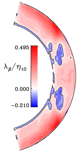
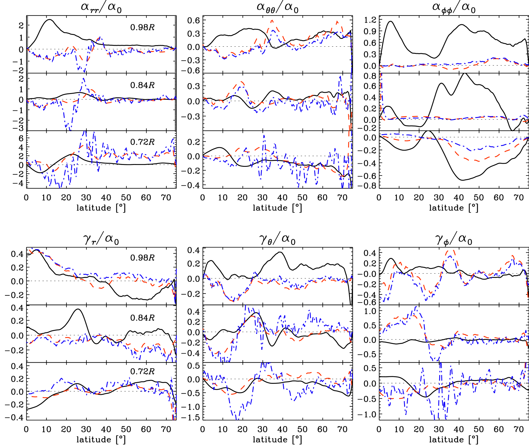
4.1 Meridional profiles of

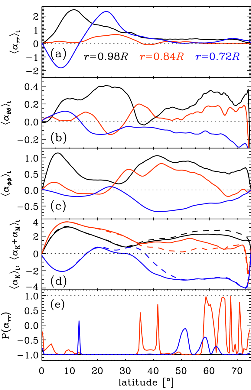
In Fig. 1 we plot the time averages of all components of . All three diagonal components of are mainly positive in the north and negative in the south, but have a sign reversal in the lower layers of the convection zone (except ). This behavior is similar to that of for isotropic and homogeneous turbulence in the low-dissipation limit (Pouquet et al. 1976) via
| (7) |
where and are the kinetic and magnetic coefficients, respectively, is the fluctuating vorticity, is the small-scale kinetic helicity, is the fluctuating current density, is the small-scale current helicity, and is the mean density. For a direct comparison we plot the meridional distributions of and in Fig. 1 as well as the latitudinal profiles of the diagonal components of together with those of and + at three different depths in Fig. 2.
It turns out that is the strongest of all components of , in particular in concentrations near the surface at low latitudes; see Figs. 1 and 2. The same has been found previously for Cartesian shear flows using both multidimensional regression methods (Brandenburg & Sokoloff 2002; Kowal et al. 2006) as well as the test-field method (Brandenburg 2005b). Unfortunately, a comparison with Käpylä et al. (2009), where transport coefficients for convection in a Cartesian box have been obtained by the test-field method, is not possible as was not determined there. In the middle of the convection zone, is much weaker than above and below; but compared to the other components of the values are still high or similar (). The latitudinal dependency shows a steep decrease from low to high latitudes.
Next, is around six and two times weaker than and , respectively, and shows multiple sign reversals on cylindrical contours; see Fig. 1. A region of negative (positive) at mid-latitudes in the northern (southern) hemisphere coincides with a local minimum of the rotation rate as seen in Fig. 1 and a maximum of negative radial and latitudinal shear (, ); see bottom row of Fig. 3. In the results of Schrinner et al. (2007, 2012) and Schrinner (2011), and have opposite signs in comparison to the present work. In their results, the and components are negative (positive) near the surface in the northern (southern) hemisphere and positive (negative) deeper down and therefore do not show a pattern similar to and as in our work. Furthermore, their and are around four times weaker than , whereas in our work is the largest.
Further, shows concentrations at low and mid to high latitudes near the surface, but also in deeper layers, where its sign is opposite to that near the surface. This sign reversal with depth is most pronounced in , but also visible in . The meridional profile of is roughly similar to that of , although its strength is smaller, see Figs. 1 and 2. This is consistent with the finding of Schrinner et al. (2007), where was similar to . Therefore a mean-field model using was not able to reproduce the magnetic field, while a model using was. The latitudinal dependencies of and follow neither a typical cosine distribution as found by, for example, Käpylä et al. (2006a) for moderate rotation, nor a distribution as often assumed in Babcock-Leighton dynamo models (e.g., Dikpati & Charbonneau 1999). In Käpylä et al. (2009), an increase of and from the equator to the poles was found, but the functional form is not clear.
The off-diagonal components of have strengths similar to and and are therefore significantly weaker than . Though of opposite sign, and have similar equatorially symmetric profiles, with positive and negative values, respectively, in the upper 75% of the convection zone – in particular below mid-latitudes. Finally, is similar to , but the sign reversal in the region of minimum at mid-latitudes is more pronounced in and at high latitudes the sign is the same. While and have the same sign, has the opposite sign compared to Schrinner et al. (2007). In general, the coefficients obtained in the present paper are less “cylindrical” than in the work of Schrinner et al. (2007, 2012) and Schrinner (2011), probably because in our simulation, rotation is slower and convection is more supercritical.
Inspection by eye already suggests that the components of are almost fully equatorially symmetric or antisymmetric333For the special solutions of the full MHD problem in a model with only -dependent coefficients, given by equatorially symmetric velocity, density and entropy with an either symmetric or antisymmetric magnetic field, it can be shown that the main diagonal components of , as well as are antisymmetric, all other components symmetric.. In order to study these symmetries quantitatively we define the pointwise parity of a quantity, for example, , as
| (8) |
where are the equatorially symmetric and antisymmetric parts of , respectively. In the bottom panel of Fig. 2, we exemplarily plot . As expected, its value is in most of the meridional plane , corresponding to antisymmetry. This is particularly valid near the surface (black line). The locations, where the parity is different coincide with values of being close to zero, and are of low significance. All other components show the same small deviations from the pure parity state and . To describe the overall parity of a coefficient by a single number , we also employed Eq. (8) with additional volume integrations in numerator and denominator; see Figs. 1, 4, 7, 9, and 16 for these values. For we have which is consistent with the almost pure overall equatorial symmetry of the velocity field444We note that the symmetric (antisymmetric) part of a vector field is constituted by the symmetric (antisymmetric) parts of , but the antisymmetric (symmetric) part of .: , , and .
4.2 Magnetic field generators
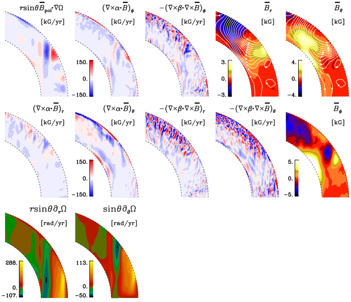
Top row, from left to right: effect , toroidal effect , toroidal turbulent diffusion , mean radial and latitudinal field , . White: Field lines of mean poloidal field . Middle row: Radial and latitudinal effect , radial and latitudinal turbulent diffusion , mean toroidal field . Bottom row: Components of . We note that the effects are computed with at the halfway point of a typical activity cycle with positive (cf. Fig. 13, top), but with the time-averaged transport coefficients (see Section 4.2).
To investigate the relative importance of the main contributions to mean magnetic field evolution in detail, we plot those from the and effects as well as from the turbulent diffusion in Fig. 3 along with the components of and the shear. Contributions from the meridional circulation have turned out to be significantly weaker; see the dynamo number calculations in Käpylä et al. (2013) and Käpylä et al. (2016a). We also do not show the contributions related to , or . Here, , and shear have been time-averaged over all cycles in the saturated stage. For we first constructed a typical magnetic cycle by folding all magnetic cycles on top of one another and averaging. Then we selected the instant at the half of the activity cycle with positive toroidal magnetic field near the surface at low latitudes and used the corresponding for the calculations.
We employ here the poloidal-toroidal decomposition of the mean magnetic field with , and being the unit vector in the direction . The effect shears the mean poloidal field, generating mean toroidal field via (top row of Fig. 3). At mid latitudes we find two distinct contributions: Outside the tangent cylinder555The cylinder aligned with the rotation axis and tangent to the sphere bounding the domain from below. the negative radial shear (see bottom row of Fig. 3) generates a negative toroidal field from the positive radial field. Further away from the tangent cylinder the sign of the radial shear changes and it produces positive toroidal field. These two regions of field production coincide well with those of strong as shown in the middle row of Fig. 3. Inside the tangent cylinder, the positive latitudinal shear generates positive toroidal field again, but weaker than the radial shear does, and we find a corresponding region of positive toroidal field. Beside these pronounced regions, there is also negative toroidal field production near the surface due to radial shear at high latitudes. However, for these regions, there seems to be no clear relation to toroidal field concentrations at this instant of the cycle.
At the same time, the effect can also generate toroidal magnetic field via ; see the top row of Fig. 3. This involves radial derivatives of and latitudinal derivatives of . One finds that the effect generates toroidal field of the same sign as the effect at mid latitudes just outside the tangent cylinder, therefore enhancing its negative toroidal field production. However, the contribution from has only one third of the strength of the effect. Directly next to this region, further away from the tangent cylinder, the effect generates positive toroidal field similar to the effect, but again weaker. Additionally, the effect is strong close to the surface, producing positive toroidal field at mid- to high latitudes (at high latitudes mostly opposite to the effect). Close to the surface at high latitudes it is comparable to the effect, while at low latitudes in the upper half of the convection zone it is locally stronger. This is suggestive of an dynamo being dominant near the surface, while the dynamo dominates in deeper layers which is supported by phase relation measurements of Käpylä et al. (2013): Equatorward migration is explained by an dynamo wave in the bulk of the convection zone (Warnecke et al. 2014), while near the surface the phase relation is consistent with an dynamo. Here, Käpylä et al. (2012) found a high-frequency dynamo mode in addition to the main mode as discussed in detail in Warnecke et al. (2014) and Käpylä et al. (2016a) for similar runs. However, the hypothetical dynamo has to be verified in a mean-field model. This result seems to be consistent with the conclusion presented in Schrinner et al. (2011), where the authors show that also has a strong contribution to the magnetic field evolution and actually sets the cycle period. However, in our simulation, the main generator of toroidal magnetic field is still the effect, in particular for the equatorward migrating field. The toroidal effect also shows negative contributions at high latitudes in the upper half of the convection zone, where it takes part in the generation of toroidal field; see top and middle rows of Fig. 3.
In the third panel of the top row of Fig. 3 we plot the toroidal contribution of the turbulent diffusion using the full , which is discussed in detail in Section 4.4. It has roughly the same strength as the main toroidal field generators, but shows the opposite sign in the mid-latitude regions of strong field production. However, it exhibits far stronger spatial variations than the corresponding and effects and thus does not match up well with the production terms. The structures at small spatial scales can be taken as indications of poor scale separation between mean and fluctuating quantities, pointing to the need of scale-dependent transport coefficients; see Section 3.1. We note here that a simplified treatment with yields excess values by a factor of three and an incorrect distribution.
We also investigated the effect generating from via ; see middle row of Fig. 3. The effect contribution to the poloidal field seems to be weaker than that of the effect to the toroidal one giving an indication of the weaker poloidal than toroidal field at mid and lower latitudes. However, in the deeper convection zone at mid to high latitudes, is comparable with . The positive radial contribution of the effect fits well with the positive radial field at mid latitudes outside the tangent cylinder. However, it generates negative radial field slightly toward higher latitudes, which has no correspondence in the radial field. At high latitudes the radial effect shows strong spatial variations producing mostly positive radial field. At low latitudes, one finds small patches of positive and negative radial field generation.
The latitudinal effect also shows field generation at mid-latitudes outside the tangent cylinder coinciding well with positive latitudinal field there. Interestingly, the latitudinal effect is particularly pronounced close to the surface, similar to the azimuthal effect. This might be an indication of a possible dynamo operating in these regions. However, the radial effect does not show such a profile. For the poloidal field, we also calculated the turbulent diffusion; see middle row of Fig. 3. As for the toroidal field, the diffusion shows strong spatial variations. At the surface the latitudinal diffusion seems to counteract the latitudinal effect. The production sites of toroidal field seem to match with the contributions shown in Fig. 3, but there are still some differences. The poloidal field production, however, cannot be linked directly to the shown production and diffusion terms, due to the phase-shift between and as shown in Warnecke et al. (2014). That is why the latitudinal effect produces negative latitudinal field, where this is positive. Furthermore, there are additional effects in the mean electromotive force (Sections 4.3–4.7), which together with the meridional flow affect the mean field.

4.3 Turbulent pumping
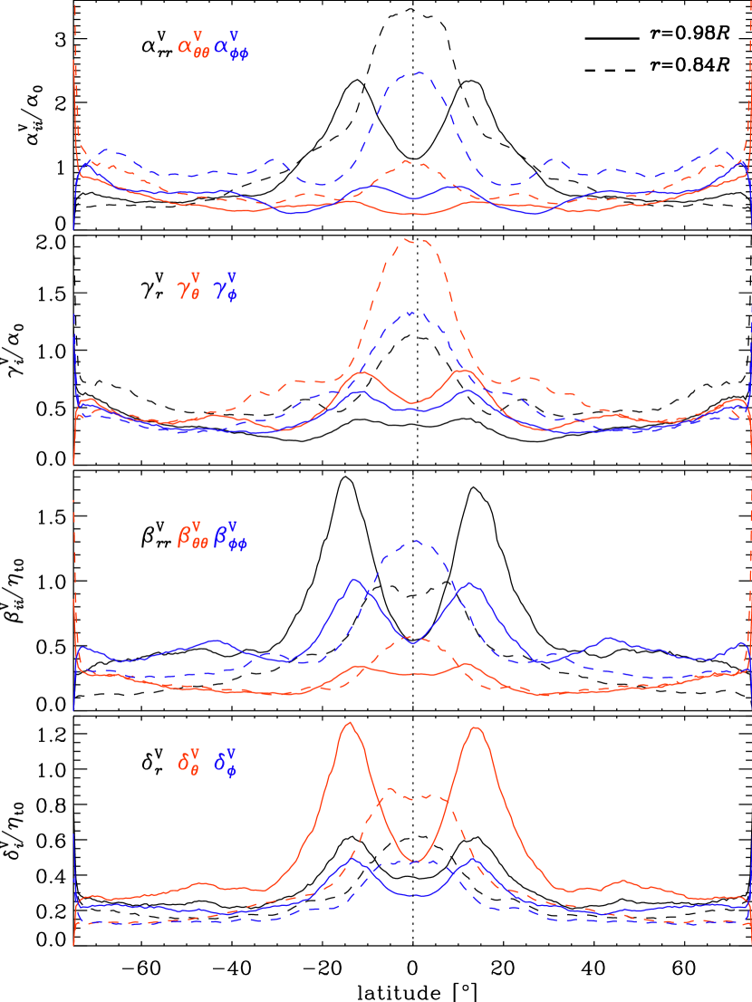
In Fig. 4, we plot the time-averaged components of the turbulent pumping velocity . The latitudinal component is the strongest with extrema of around of the turbulent velocity . The other components have a half () and a third () of the values. Hence all components are comparable to the off-diagonal components of , while being three () to ten () times weaker than .
For there are two distinct regions: Inside and close to the tangent cylinder, is mainly negative (except at high latitudes in the middle of the convection zone), whereas further outside it is mainly positive. Close to the surface, at low and mid-latitudes, is positive indicating outward pumping of magnetic field. This is at odds with downward pumping found in local simulations of the near-surface layers (e.g., Nordlund et al. 1992; Ossendrijver et al. 2002), but in agreement with what is expected from SOCA or even earlier calculations, where the pumping is proportional to the negative gradient of the turbulence intensity () (e.g., Kichatinov 1991). In a study using scale-dependent one-dimensional test fields in Cartesian convection simulations, Käpylä et al. (2009) found that downwards pumping occurs only for uniform () mean fields and outward pumping for all other field scales (). We find, however, that at high latitudes near the surface downward radial pumping dominates. The difference between high and low latitudes can be due to rotational influence. The negative extrema of occur near the bottom of the convection zone close to the tangent cylinder. The positive extrema seem to be correlated with negative radial shear (bottom row of Fig. 3) or appear close to the surface in the equatorial region. With overall parity , the equatorial symmetry of is close to perfect.
The latitudinal component is antisymmetric with respect to the equator (). It is negative (positive) in the northern (southern) hemisphere in the lower half of the convection zone, with extrema close to the tangent cylinder, while in the upper half of the convection zone its sign is mostly opposite. This means that turbulent pumping is poleward in the lower half of the convection zone and equatorward in the upper half, as also indicated by the streamlines of in Fig. 4. Interestingly, the pumping is strongly equatorward in the same region where equatorward migration of the toroidal field is caused by the negative shear; see Figs. 1, 3 and 4 and compare with Figs. 3 and 4 of Warnecke et al. (2014).
The azimuthal component is close to being equatorially symmetric (). It is positive near the surface at low to mid latitudes as well as near the tangent cylinder at low latitudes, otherwise negative with minima just inside the latter (see Fig. 5 for in physical units). All components show strong similarity with the turbulent pumping coefficients presented in Schrinner et al. (2007, 2012); only in the upper half of the convection zone and in particular near the surface do we find a different behavior.
To understand the effects of the off-diagonal components of , Kichatinov (1991), Ossendrijver et al. (2002) and, for example, Käpylä et al. (2006a) have advocated a view of component-wise pumping in which three different pumping velocities , acting on the Cartesian component fields666No summation over is applied here. , are identified. Under the condition that the latter are all solenoidal and the former are spatially constant, it can be shown that each component field is advected as . In the present context, however, neither of the stated conditions is satisfied. Given that the poloidal and toroidal constituents of are solenoidal, we consider their evolution separately, focussing on the terms related to turbulent pumping and mean velocities
| (9) | ||||
Thus, in the absence of all other effects, both and are frozen into (but not advected by) the “effective” mean poloidal velocity , while the toroidal field is, in addition, subject to the source term , , representing the winding-up of the poloidal field by the simultaneous effect of differential rotation and toroidal pumping .
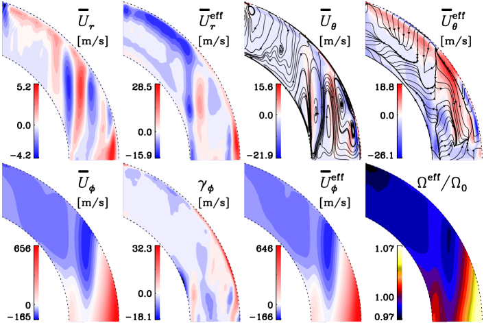
We show the temporally averaged effective mean velocities in comparison to alone in Fig. 5. For (upper row), turbulent pumping has a significant impact: at high (low) latitudes its radial component is dominated by the strong downward (upward) pumping such that there, , while at the tangent cylinder, , and the equatorward flow in the upper half of the convection zone is also significantly enhanced. Close to the surface the effective velocity has a strong equatorward component. As a consequence, the whole meridional circulation pattern, as shown by the streamlines in Fig. 5 is changed: The three meridional flow cells aligned with the rotation vector outside the tangent cylinder are no longer present in . We note that, while at least is solenoidal, no such constraint applies to and, hence, neither to . Near-surface patches of poloidal flux may, in principle, be able to reach the bottom of the convection zone when transported by the meridional circulation , albeit on a rather involved route. However, this can hardly be accomplished by the effective meridional circulation mainly due to its massive deviations from solenoidality. Consequently, the flux transport dynamo paradigm seems to be inconsistent with the presented simulations. Even if helioseismic inversion were to determine accurately the meridional circulation inside the solar convection zone, the effective meridional velocity would still be unknown, because one cannot measure inside the Sun.
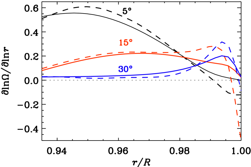
The azimuthal flow and hence the differential rotation is only marginally modified by (see Fig. 5, bottom row). However, at the surface it affects the radial shear significantly, as shown in Fig. 6, where we plot the radial derivatives of the rotation rate and its effective counterpart . At low latitudes, the effective radial derivative becomes negative whereas at mid latitudes it is weakly enhanced. We note that simulations of the type employed here do not produce a negative radial derivative as found in the Sun (Käpylä et al. 2013; Warnecke et al. 2016a) where near the surface (e.g., Barekat et al. 2014) being possibly responsible for the equatorward migration of the toroidal field (e.g., Brandenburg 2005a). Also, at this location the toroidal turbulent pumping can modify the effective radial shear and thus the magnetic field generation. Schrinner et al. (2012) concluded that their radial and latitudinal turbulent pumping show a strong influence on the magnetic field generation. This effect was reported to become stronger for faster rotation. However, the authors did not consider the effect of azimuthal turbulent pumping, which can modify the effect.


4.4 Turbulent diffusion , effect, and term
In Fig. 7 we plot all components of the time-averaged and tensors. All diagonal components of are mostly positive. Overall, the values of are significantly smaller than the turbulent diffusivity estimate with the exception of reaching 1.37 at the tangent cylinder near the surface. These regions are also pronounced in , but its values are only around half as large. With values still five times smaller than , is strongest at high latitudes. The apparent dominance of amongst the diagonal components is partly an artefact of the ambiguity in defining the tensors in Eq. (4) based on those in Eq. (6); see Schrinner et al. (2005). Effectively, and should be multiplied by a factor of two for comparison with ; see the discussion of at the end of this section. The overall parities of the diagonal components approach the ideal value (), while those of the off-diagonal components are still close () with and being close to antisymmetric and close to symmetric. In the northern hemisphere, is negative in the lower half of the convection zone and positive in the upper half. The contours of are approximately aligned with the rotation axis, showing a clear sign reversal outside the tangent cylinder such that the sign of is anti-correlated with that of the latitudinal shear; see bottom row of Fig. 3. is particularly strong (positive) only near the equator. In the geodynamo model of Schrinner et al. (2007), the diagonal components show a strong alignment and concentration near the tangent cylinders, while in our work the components are most prominent at high latitudes and around the local minimum of . Of the non-diagonal components, () is similar outside the tangent cylinder, () is similar in the lower half of the convection zone, and () shows the opposite sign with a similar pattern.
For inspecting the energetics of the system, it is interesting to study whether or not is positive definite, that is, whether or not the effect of the term onto is exclusively dissipative. We note that such a study was not performed in previous works (Schrinner et al. 2007, 2011, 2012). To this end, we calculated the eigenvalues of and depict the third root of their product in Fig. 8. It is predominantly positive, adopting negative values only at lower latitudes, and with less than half the moduli compared to the maximum. We note that this finding is not contradictory to any basic principle as negative turbulent diffusivities have been conclusively demonstrated to exist, albeit in laminar model flows only (Devlen et al. 2013). Comparison with the field generators in Fig. 3 suggests that a possible generative effect from the negative definite is most likely weak.
The coefficient is known to parameterize the “ effect” appearing already in homogeneous anisotropic non-helical turbulence (Rädler 1969, 1976) when the preferred direction is given by that of the global rotation. may also contain a contribution from the “shear-current effect” which occurs already in homogeneous non-helical turbulence under the influence of large-scale shear (see, e.g., Rogachevskii & Kleeorin 2003, 2004). We note that the major physical difference between turbulent diffusion and the effect is that the latter does not lead to a change in mean field energy as .
The coefficient shows no preferred sign for any of its components; has the same pattern as (contours aligned with the rotation axis, sign reversal), but opposite values. is strongest close to the equator with negative values near the bottom and the upper part of the convection zone and positive values in between and near the surface. and are around two times larger than , which is mostly negative (positive) in the northern (southern) hemisphere outside the tangent cylinder and positive (negative) inside. The overall parities of () are comparable with those of the off-diagonal components of with being symmetric and and antisymmetric. We find that the contribution of the effect on the generation and amplification of the magnetic field is small compared to the other terms discussed in Section 4.2. Similarly as for , all components are consistent with previous studies (Schrinner et al. 2007); is similar outside the tangent cylinder, while and are only similar in the lower half of the convection zone.
The components of the rank-three tensor can be reduced from 27 to 15 independent components777By adopting symmetry in the last two indices and dropping .; see Fig. 9 for the results of the current simulation. All components are below with the most dominant ones being , , , , . Several of the profiles show alignment with the rotation axis. The parity of all components of () is similar to those of the off-diagonal components of . We note here that considerable dissipative effects are “hidden” in the term. This can be seen by exploiting the freedom in defining the components ; see Eq. (3): They can be chosen such that and adopt twice their values. One can even go further and employ a choice by which all off-diagonal components of disappear. The corresponding value of has then a maximum; of 1.7 instead of 0.495 (cf. Fig. 8), indicating that the turbulent diffusion is actually stronger by a factor . Of course, changes in the choice of the influence, in general, all transport coefficients.
4.5 Variations in time
The transport coefficients show a strong variability in time and can hence be divided into a constant (= time-averaged) part and a part with temporal average zero, called variation (indicated by superscript ), such as
| (10) |
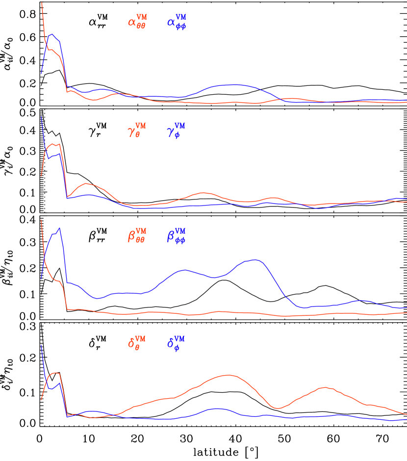
In Fig. 10, we plot the rms values of the variations, defined as
| (11) |
(we emphasize the capital V in the symbol). For all shown coefficients these are stronger at lower- than at higher latitudes. Near the surface () the variations have their maxima around latitude. This distribution indicates a strong influence of the mentioned poleward migrating high-frequency constituent. However, in the middle of the convection zone () the maxima are around the equator, where the high-frequency constituent is not present (Käpylä et al. 2016a). In addition, at mid to high latitudes, the variations also show significant values. The variations of and are roughly equal to their time averages near the surface, but significantly bigger in the middle of the convection zone near the equator. Furthermore, and are significantly stronger than and , respectively, but is only about one half of . The variations of the also exceed their time-averages by several times. In his PhD thesis, Schrinner (2005) also presented the standard deviations of the transport coefficients for a time-dependent dynamo. There, he found values of a relative strength of 0.4 to 0.7 for the diagonal components, which is somewhat lower than what we find. However, the convection in his simulation was not as vigorous as in ours. Thus, we can conclude that the time variation of the coefficients may play an important role in the evolution of the magnetic field. Further analysis shows that the variation distributions can be modeled by Lorentzian profiles and are therefore consistent with a random process. However, the variations also have non-random contributions, which show tight relations to the mean magnetic field evolution. This is discussed further in Section 4.7.
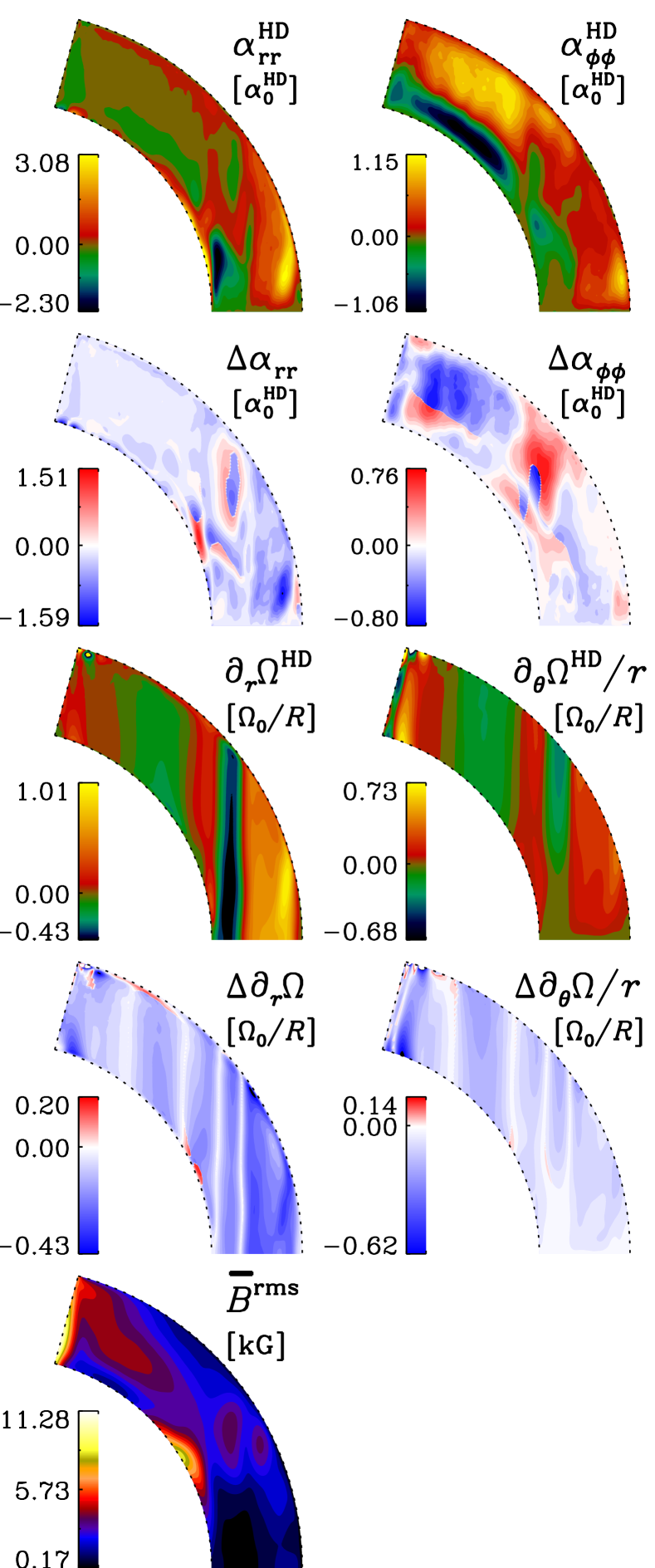
from HD, from MHD and HD, radial and latitudinal shear , from HD, , from MHD and HD, (rms over full time series). The quantities contain the sign of the corresponding HD quantities to highlight enhancement (red) and quenching (blue).
4.6 Magnetic quenching
To investigate the alteration of the transport coefficients by the mean field, we first compare the MHD run to the corresponding HD run. In Fig. 11, we show the absolute differences of the time-averaged dominant diagonal components and , employing the quantity . Here, multiplying with the sign allows to distinguish between enhancement (red) and quenching (blue). is mostly quenched, in particular at low latitudes. shows enhancement in the region of strong negative latitudinal shear, and also in the lower half of the convection zone at high latitudes. Strong quenching of occurs mostly at high latitudes, where the rms value of the mean field is particularly strong; see the last row of Fig. 11.
The other quantities also exhibit alterations due to the presence of the magnetic field (not shown here). The upward pumping near the surface is much stronger in the MHD case compared to the HD one whereas at high latitudes is suppressed. and are also suppressed in the region of strong negative radial shear and strong toroidal field at mid and high latitudes. and are, in general, suppressed compared to the HD case, in particular near the surface at mid-latitudes. However, they exhibit enhancement in the regions with strong toroidal field and negative shear at mid-latitudes where and are suppressed while being enhanced everywhere else. turns out to be enhanced everywhere. In comparison with the HD case, is suppressed in the proximity of the tangent cylinder and at high latitudes. Similarly to , is suppressed near the surface at low latitudes and in the region of negative shear.
As indicated by the quantities , defined analogously to , the shear is also quenched, similar to what is seen in, for example, Brun et al. (2005), Busse & Simitev (2006), Aubert (2005), Gastine et al. (2012) and in particular recently for models of solar-like stars (e.g., Fan & Fang 2014; Karak et al. 2015; Käpylä et al. 2016a, 2017). This means that the quenching of the turbulence by the mean field results in the modification of both the differential rotation generators (Karak et al. 2015) and the mean . Therefore, along with its direct influence via the fluctuating velocity, the mean field also has a more indirect effect on the transport coefficients via the mean flows.
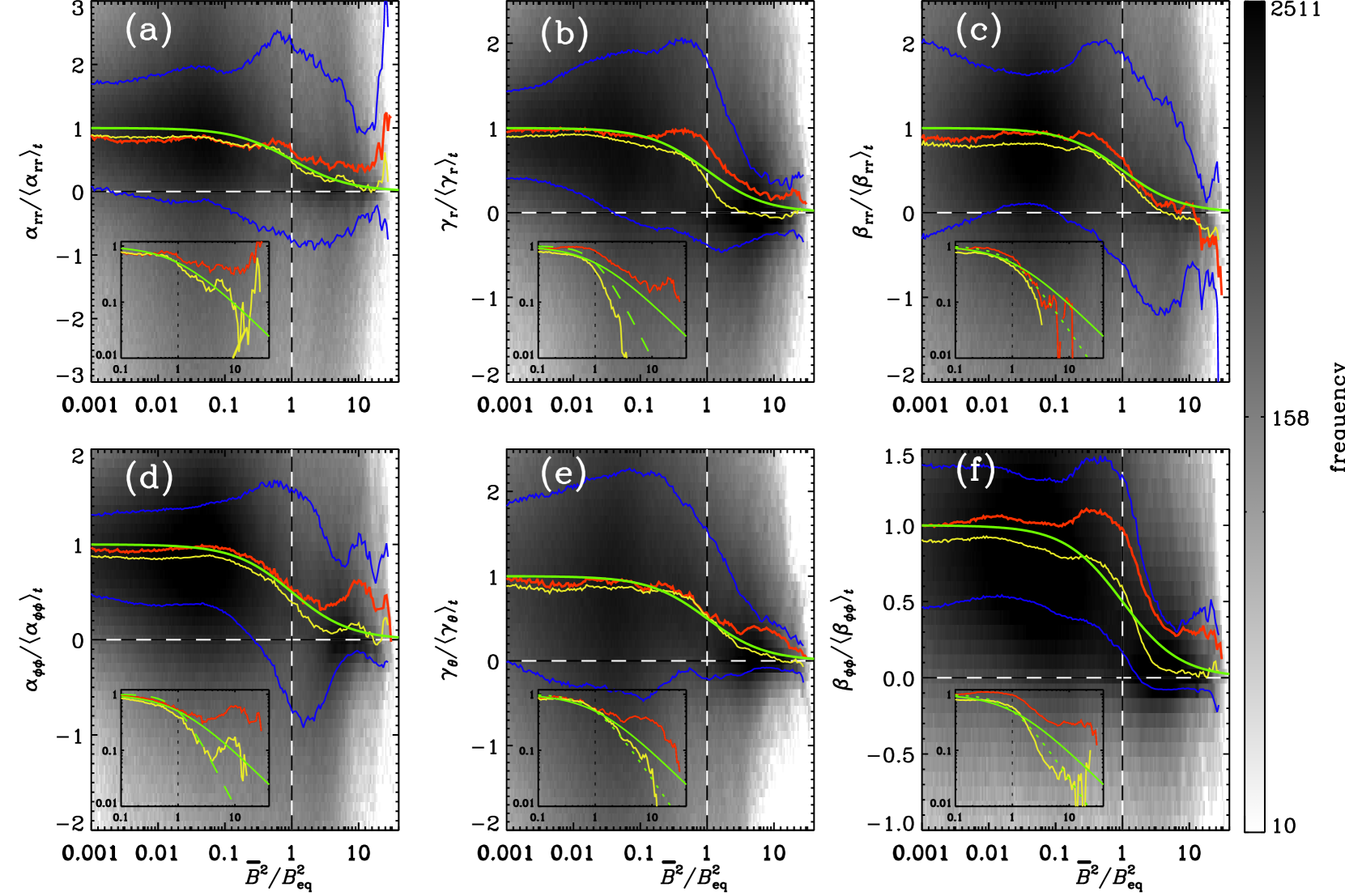
Given the strong variability of the mean field both in space and time, we suggest using the corresponding variability of the transport coefficients for deriving their functional dependencies on the mean field, thus opening the gateway to predictive mean-field models. Unfortunately, we have to expect that these dependencies involve complex and nonlocal relations not only with the mean field, but also with its derivatives, for example, the mean current density. Currently, no appropriate mathematical model and hence no numerical scheme identifying these relations is available. However, a starting point could be the model of Rheinhardt & Brandenburg (2012) with - and -dependent coefficients in the evolution equation for . Here we restrict ourselves to establishing a rough relationship between the magnitudes of the transport coefficients and the modulus of the mean field including all points in the domain and all instants in time. Of course we cannot hope to find anything close to unique functional dependencies. Instead, for a certain field strength many different values of a transport coefficient are found across the spatio-temporal domain. Hence, if at all, relationships can only be identified in a statistical sense.
In Fig. 12, we plot 2D histograms of some of the most important coefficients depending on the energy density of the mean field, normalized by its equipartition value . For this, the whole saturated stage (18 activity cycles) was considered, while smoothing the coefficients over six points in space and time ( a tenth of an activity cycle). We use 200 bins for both the normalized coefficients (in the interval ) and the normalized field (in the interval . Although the scatter is large, in most of the coefficients there is significant quenching detectable where the mean field becomes dynamically important (). The average and median values for weak mean field are slightly below the time-averaged quantities, but we still use the latter as proxies for the unquenched values.

The coefficient in Fig. 12(a) is quenched for , with the median following approximately a quadratic characteristic . For stronger fields, median and mean show inconclusive behavior, including both enhancement and quenching, and hence do not follow any simple analytic dependency. For , Fig. 12(d), the behavior is similar, albeit with a median closer to quartic behavior . , Fig. 12(b), shows even enhancement until , but then a decrease in mean and median with a less-than-quadratic and stronger-than-quartic characteristic, respectively. The median of the latitudinal pumping , Fig. 12(e), follows a cubic characteristic relatively closely, but with a much shallower-than-quadratic mean. For the turbulent diffusion, Fig. 12(c) and (f), the coefficients are enhanced below and decrease then with quadratic or even cubic decline (in the medians). To summarize, none of the coefficients follow exactly one single analytical quenching formula.
Schrinner et al. (2007) studied the quenching of the turbulent transport coefficients not by comparing with a purely hydrodynamic run or employing a time-dependent magnetic field, but used a series of simulations with increasing magnetic field strengths. They found that and all diagonal components first increase with growing magnetic field, but decrease when the Lorentz force becomes comparable to the Coriolis force.
4.7 Cyclic variation
As a consequence of the cyclic variation of the mean field, the transport coefficients also vary cyclically. In Fig. 13, we plot the cyclic variations of the diagonal components of and , along with , and the corresponding toroidal and radial mean field for a typical cycle, the definition and computation of which was described in Section 4.2. By folding the cycles on top of one another, one basically filters out the variation based on the cyclic magnetic field. To distinguish the cyclic variations from the time variations discussed in Section 4.5, we add the superscript “M” to the symbols; for example, . All coefficients show clear cyclic variations with the activity cycle period (= half the magnetic cycle period), owed to the quadratic effect of the mean field on the velocity fluctuations. In many cases, this is clearly visible at high latitudes. and seem to be predominantly quenched by the toroidal field, while , , , , and the shown components of seem to be predominantly quenched by the radial field as indicated by the pattern at high latitudes. At lower latitudes, the variations exhibit time scales shorter than the activity cycle, which cause a noisy signal when folding the cycles. The fast poleward migrating constituent of near the surface at low latitudes (ghosts of which are visible in Fig. 13), discussed in Warnecke et al. (2014) and Käpylä et al. (2016a), is one candidate for causing such a signal. As discussed in Käpylä et al. (2016a) for a similar run, this high-frequency dynamo mode is highly incoherent over time, that is, cycle length and phase change on short time scales, which could well be the cause of the noisy appearance when averaged over several cycles.
To quantify the variations further, in Fig. 14 we plot their rms values, defined analogously to Eq. (11). For all shown coefficients, the cyclic variations are around four times smaller than the non-cyclic variations; they are, however, still comparable with the time-averaged values. Also here the coefficients vary more strongly at lower than at higher latitudes. The variation in the components of and are stronger than in the other components. Otherwise, the behavior and values of all components seem to be similar. Given that the relative cyclic variations in the mean flows are at most around 10 (see the discussion in Käpylä et al. (2016a)), we conclude that the back-reaction of the mean field onto the terms generating it is predominately via the variation of the transport coefficients.
4.8 Magnetic field propagation
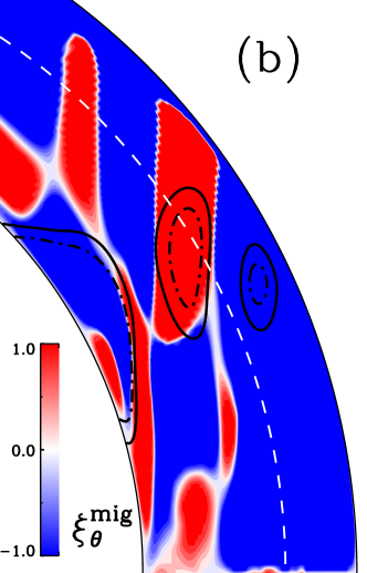

(b) and c): Latitudinal propagation direction of the mean field as predicted by the Parker-Yoshimura rule (12), using (b) and (c, see Section 4.9), together with as black contours for 3 (solid) and 3.5 kG (broken). The color scale is truncated between and 1 to emphasize the sign of . The dashed white lines indicate .
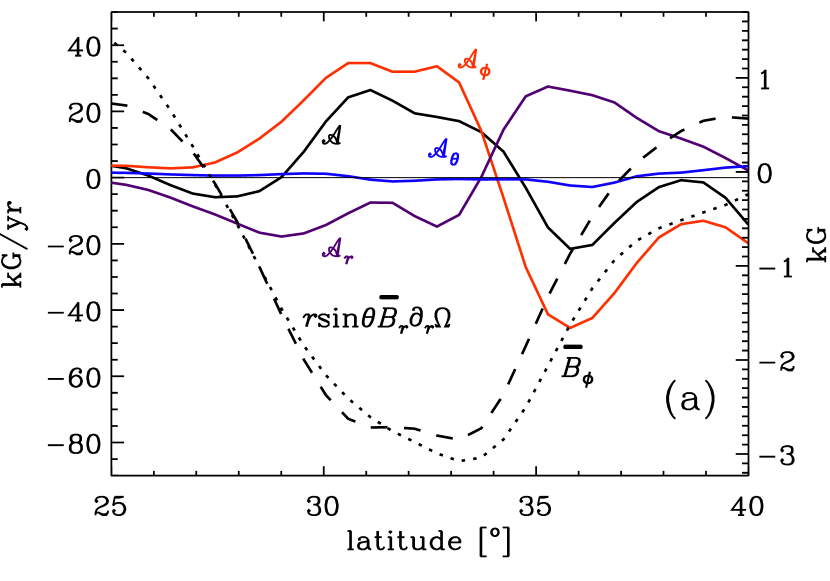
As discussed in Warnecke et al. (2014), the occurrence of the equatorward-propagating magnetic field found in Käpylä et al. (2012) can be well explained by the Parker-Yoshimura rule (Parker 1955; Yoshimura 1975) using as the relevant scalar . For the rule to be applicable, the effect must be dominant over the toroidal effect, and the poloidal effect must be expressible with a single (possibly position-dependent) scalar by . Having now all transport coefficients at hand allows us to investigate why the Parker-Yoshimura rule provides such a good description. To show this, we focus on the mid-latitude region where the shear is negative, causing the generation of equatorward migrating toroidal field . There, the contribution to the effect dominates the generation of the toroidal field. So the radial component is the important part of the poloidal field in the dynamo wave. In Fig. 15(a) we plot the contributions to the radial effect , named , , and and defined in the caption. The latitudinal effect shows a similar behavior. Obviously, the contribution related to (, red line) is indeed dominant in the region where the toroidal field and the negative shear are strong. Consequently, we now use to determine the equatorward propagation direction:
| (12) |
Figure 15(b) shows that the result is consistent with the actual propagation direction.888The rule does not exclude dynamo waves propagating along directions inclined with regards to the isocontours of . The highest growth rate, however, occurs for aligned propagation. We note that in the saturated nonlinear stage, a kinematically subdominant mode may nevertheless be prevalent. Using instead of works for this run only by chance as their signs are the same in the region of interest. However, in general, the Parker-Yoshimura rule using will not always work as other components of may give more important contributions. Parker dynamo waves have also been found in numerous Boussinesq (e.g., Busse & Simitev 2006; Schrinner et al. 2012) and anelastic dynamo simulations (e.g., Gastine et al. 2012). In particular, in these studies it was found that the oscillation frequency can be well described by a simplified dispersion relation of the Parker dynamo wave. To show that the magnetic field propagation in our simulation is consistent with a Parker dynamo wave, we estimate its period, as described by Parker (1955) and Yoshimura (1975), using a wave ansatz which leads to the frequency
| (13) |
where we only consider latitudinal propagation. With , we obtain periods of two to four years in the region of interest, which is close to the actual period of around five years. As investigated in detail by Käpylä et al. (2016a) and Olspert et al. (2016) for a similar run, the main dynamo mode, present in the upper and middle part of the convection zone, shows a strongly variable cycle period that remains coherent only over two to five cycles, with values of between four and eight years. The value of is a lower limit and a higher one might be more reasonable, which would lead to a shorter period, while still retaining the correct order of magnitude. Taking into account the strong simplifications leading to Eq. (13), for example the neglect of anisotropic contributions to , the predicted period fits the actual one rather well.
4.9 Comparison with multidimensional regression method
In Brandenburg & Sokoloff (2002), a method for determining the transport coefficients has been used which is based on the temporally varying mean magnetic field of the dynamo (the main run) alone (called BS method in the following). Instead of solving additional test problems with predefined mean fields as described in Section 3, the method exploits the fact that at different times at a given position has, in general, different directions. So using sufficiently many time instants, the underdetermination of Eq. (6) can be overcome. One can go further and employ any available instant ending up with a (usually heavily) overdetermined system which can be solved approximately by the least-squares technique or singular value decomposition. An intrinsic problem emerges when reaches dynamically relevant strengths: Then the transport coefficients become dependent on and would be determined in a temporally averaged sense where, however, it remains unclear to which strength of their values correspond. Clearly, the BS method does not allow to obtain information on the time evolution of the transport coefficients. Furthermore, some of the coefficients calculated in Brandenburg & Sokoloff (2002) have turned out not to be in agreement with test-field results. This especially concerns the components of the turbulent diffusivity tensor acting on currents along and perpendicular to the shear, which are correctly obtained only with the test-field method (Brandenburg 2005b).
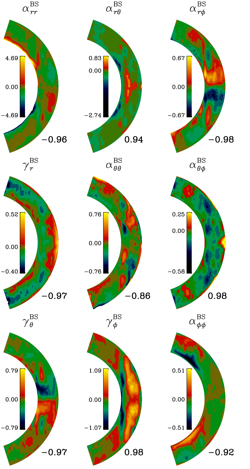
In several papers (Racine et al. 2011; Simard et al. 2013; Nelson et al. 2013; Augustson et al. 2013, 2015), the BS method was severely simplified in that in Eq. (6) the contributions with derivatives of were dropped, that is, , and were set to zero (called reduced BS method in the following). Such a modeling can hardly be expected to offer any predictive power as already turbulent diffusion is not modeled in a proper way. Accordingly, when employing the coefficients found in this way, one has to add turbulent diffusion by hand in order to obtain reasonable growth rates. With respect to descriptive power, this method must also fail as the individual, interpretable turbulent effects are all subsumed in one tensor. Recently, Simard et al. (2016) used the full BS method and compared the coefficients for one of their simulations with the reduced BS method. They found the and tensors to be nearly the same in both cases and their values of to be much smaller than their .
Here we demonstrate that indeed the and coefficients derived with the (reduced) BS method do not show correspondences to those derived by the test-field method; see Fig. 16 and for more details Fig. 17. Comparison reveals that in many cases not even the signs are correct, for example, is negative in the northern hemisphere, close to the equator, where is strongly positive; see Fig. 1. We also note the much smaller spatial structures in Fig. 16 compared to Figs. 1 and 4. Furthermore, we also find that the reduced and the full BS give very similar results for the and tensor. This confirms their limited use for modeling and analysis purposes. It also indicates that the significantly smaller values of , compared to , found by Racine et al. (2011) and Simard et al. (2013, 2016) with the setup of Ghizaru et al. (2010) (see a comparison in Appendix A of Käpylä et al. 2017), are not due to particularities of the latter, but are a particular outcome of this method. Therefore most of the conclusions derived from and in the papers cited above are to be considered misleading. In particular, the conclusion of Augustson et al. (2015) that their equatorward migrating field is not well explained by the Parker-Yoshimura rule is most likely unreliable. As becomes obvious from Fig. 15(c), using instead of in Eq. (12) will lead to an incorrect prediction of the propagation direction.
5 Conclusions
We have determined the full tensorial expressions of the transport coefficients relevant for the evolution of large-scale magnetic fields from a solar-like fully compressible global convective dynamo simulation using the test-field method. The simulation used here exhibits a large-scale magnetic field with solar-like equatorward propagation similar to the runs of Käpylä et al. (2012, 2013, 2016a, 2017). This behavior can be well explained with the Parker-Yoshimura rule of an dynamo wave, where the negative shear at mid latitudes generates the mean toroidal magnetic field (Warnecke et al. 2014). However, we find indications that, locally, the effect is comparable to or stronger than the effect in generating toroidal magnetic field. This suggests an dynamo operating locally in addition to the dynamo. This is mostly due to the dominance of among all coefficients of . The meridional profiles of the coefficients do not agree with estimates based on helicities or simple profiles.
The most interesting results come from the turbulent pumping velocities. They significantly alter the effective meridional circulation and shear acting on the mean magnetic field. Most strikingly, the pattern of three meridional flow cells outside the tangent cylinder disappears completely. Furthermore, the radial turbulent pumping at the surface is upward near the equator and downward at higher latitudes and therefore in agreement with test-field results of Cartesian convection (Käpylä et al. 2009) near the equator. This has consequences also for possible dynamo mechanisms in the Sun. Even if helioseismic measurements revealed a meridional circulation pattern in favor of the flux transport dynamo (see e.g., Hazra et al. 2014), the unknown turbulent pumping velocity would be able to completely change the effective meridional circulation, in particular as the effective velocities do not have to obey the conservation of mass. Also the shear is altered by the presence of turbulent pumping, however the effect is not as strong as for the meridional flow.
For the turbulent diffusion, we find that also has a small negative definite contribution, which can potentially lead to dynamo action. However, in this particular simulation, it seems to play only a minor role. In general, the equatorial symmetry of all time-averaged coefficients agrees well with what is expected from equatorial symmetric flows.
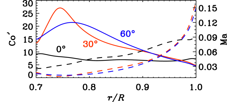
If we compare the transport coefficients determined in this work with those of previous studies of the geodynamo (Schrinner et al. 2007, 2012; Schrinner 2011), we find that most of the components agree well in the lower part of the convection zone, but disagree in the upper part. We highlight that the time-averaged and have the opposite sign and are stronger everywhere. We associate the agreement in the lower part of the convection zone of our simulation with stronger rotational influence and weaker effects of compressibility and stratification than in the upper part and surface region; hence the better fit with the mentioned studies. In Fig. 18 we plot the radius- and latitude-dependent Coriolis and Mach numbers; this clearly shows the presence of two regimes: For mid and high latitudes, the rotational influence is significantly stronger in the lower part of the convection zone than near the surface. In that region, Coriolis numbers999 We use with and from Schrinner et al. (2012). This gives for their models 4, 29, 31, and 34. estimated from Schrinner et al. (2012) fit well with our values for most of their models. Furthermore, the Mach number decreases by about one order of magnitude from the surface to the bottom of the convection zone; see Fig. 18. This indicates that in its lower part, compressibility is less important than near the surface.
The coefficients are altered by the presence of the magnetic field. Comparison with a non-magnetic simulation reveals a quenching for most of the coefficients and for the differential rotation. However, there exist also enhancements at some localized regions for some of the coefficients. In the magnetic simulation itself, we found that the coefficients are altered at the locations where the magnetic field is dynamically important. Most of the coefficients are quenched for strong magnetic fields, but for example and also show enhancements, when the field is in equipartition with the turbulent flow. No simple algebraic expression that depends on the magnetic field strength would be able to reproduce this kind of behavior. Furthermore, we find a clear cyclic modulation of all coefficients, in particular at high latitudes where the magnetic field is the strongest. Some of the coefficients seem to be quenched predominantly via the toroidal magnetic field (e.g., , ) and others via the radial field (e.g., , , , , ).
The overall strength of the temporal variations is comparable with or even larger than the time-averages of the quantities, suggesting a strong contribution to the magnetic field evolution via these variations; they are predominantly random, but also show some response to the activity cycle, that is, the cyclic change in the magnetic field. These cyclic variations are significantly stronger than those of the mean flows indicating that the nonlinear feedback occurs predominantly via the transport coefficients and not via the mean flows.
The finding of Warnecke et al. (2014, 2016a) that the Parker-Yoshimura rule can well predict the propagation direction of the magnetic field can be verified because (1) the radial effect dominates the toroidal field generation, (2) has the strongest contribution to the radial effect, and (3) has the same sign as in the region of interest. However, we find that the latitudinal derivative of also plays a significant role. Therefore, a detailed analysis for every simulation is necessary.
We also compare the test-field method with the one used by Racine et al. (2011) and Simard et al. (2013), which is based on a multidimensional regression method introduced by Brandenburg & Sokoloff (2002). Their method gives incorrect results leading to, for example, the opposite sign of and the incorrect propagation direction from the Parker-Yoshimura rule.
For followup work, we plan to use the determined transport coefficients in mean-field simulations to investigate in detail their effect and their descriptive power for the magnetic field evolution. We also plan to investigate how the coefficients, and therefore the dynamo mechanism, change by changing rotation, stratification and magnetic, fluid, and entropy diffusivities. Furthermore, it would be interesting to study the effects of a realistic treatment of the outer magnetic boundary (Warnecke et al. 2011, 2012, 2013a, 2016a) as well as the effect of the spontaneous formation of magnetic flux concentrations (e.g., Brandenburg et al. 2013; Warnecke et al. 2013b, 2016b; Käpylä et al. 2016b).
Appendix A Reconstruction of the electromotive force
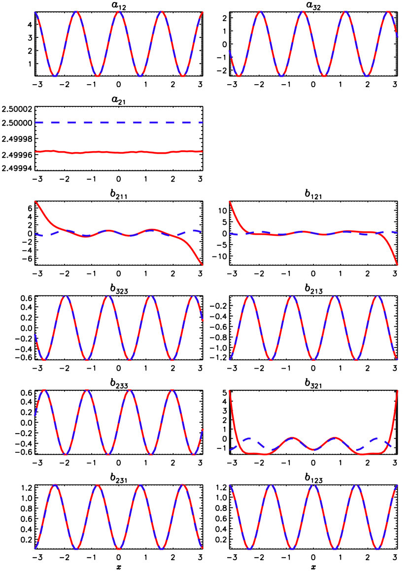
To show that the reconstruction of the turbulent electromotive force, employing the turbulent transport coefficients and here being labeled , agrees reasonably well with the directly obtained (“original” ), we plot in Fig. 19 both quantities in the middle of the convection zone. The location of strong activity at around latitudes is well reproduced in all components. Furthermore the polarity reversals at high latitude agree well in the original and reconstructed . Close to the equator, the agreement degrades: In the original we find a stationary positive pattern in the radial component and an asymmetry across the equator in the latitudinal one, but this pattern is not reproduced in . Furthermore, the absolute strength of the original is only nearly half of that of . If we reconstruct the electromotive force from the time-averaged turbulent transport coefficients (), the absolute values are closer to the original ones, but still around 30% larger. In all, seems to give a better reconstruction than , but the large random variations in time might blur the comparison (see Section 4.5). We associate the differences between reconstructed and original with lack of scale separation, that is, non-locality in space and time (Brandenburg et al. 2008b; Hubbard & Brandenburg 2009; Rheinhardt & Brandenburg 2012) and will address these issues in forthcoming publications.
Appendix B Comparison with mean-field model
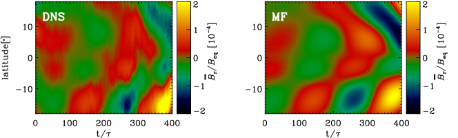
To show how well the transport coefficients describe and predict the mean magnetic field, we performed additional direct numerical simulations (DNS) producing an oscillating spherical dynamo from forced turbulence. The setup is similar to Mitra et al. (2010), but with forcing wavenumber , where corresponds to the shell thickness, and , . We computed the turbulent transport coefficients using the presented method and solved a corresponding mean-field model, which reproduces three key features of the field evolution in the DNS: (1) The growth rate of the magnetic field (, for the volume averaged rms field), (2) its oscillation period (, ) and (3) its complex latitudinal distribution. Fig. 20 shows the radial mean magnetic field as a function of time and latitude from both the DNS and the mean-field model. It is rather expected that the correspondence is very good in this case, as the scale separation is high and the Reynolds numbers are small. In our compressible convection simulations these conditions are no longer fulfilled, hence non-local effects in space and time likely play an important role. Therefore, comparison to mean-field models is less trivial and will be addressed in detail in a forthcoming publication.
Appendix C Comparison with analytical results
For comparison with analytic results we have chosen the flow
| (14) |
in a Cartesian () domain, out of a family of three, introduced by Roberts (1970); see Rheinhardt et al. (2014) for comparison. Here, and are constant prefactors and is the horizontal wavenumber of the flow. Under SOCA and for , we obtain, with averaging over , for the coefficients of Eq. (3),
| (15) | ||||
| (16) | ||||
| (17) | ||||
| (18) | ||||
| (19) | ||||
| (20) | ||||
| (21) |
Figure 21 shows these profiles in comparison with the results of the test-field method applied in Cartesian geometry. To enable maximal agreement, the non-SOCA term of Eq. (5) was switched off in the code.
Acknowledgements.
The authors thank the referee Ludovic Petitdemange for numerous useful comments and suggestions, which improved the paper. The simulations have been carried out on supercomputers at GWDG, on the Max Planck supercomputer at RZG in Garching, in the HLRS High Performance Computing Center Stuttgart, Germany through the PRACE allocation “SOLDYN” and in the facilities hosted by the CSC—IT Center for Science in Espoo, Finland, which are financed by the Finnish ministry of education. J.W. acknowledges funding by the Max-Planck/Princeton Center for Plasma Physics and from the People Programme (Marie Curie Actions) of the European Union’s Seventh Framework Programme (FP7/2007-2013) under REA grant agreement No. 623609. This work was partially supported by the University of Colorado through its support of the George Ellery Hale visiting faculty appointment, the Swedish Research Council grants No. 621-2011-5076 and 2012-5797 (A.B.), and the Academy of Finland Centre of Excellence ReSoLVE 272157 (J.W., M.R., S.T., P.J.K., M.J.K.) and grants 136189, 140970, 272786 (P.J.K).References
- Aubert (2005) Aubert, J. 2005, J. Fluid Mech., 542, 53
- Augustson et al. (2015) Augustson, K., Brun, A. S., Miesch, M., & Toomre, J. 2015, ApJ, 809, 149
- Augustson et al. (2013) Augustson, K. C., Brun, A. S., & Toomre, J. 2013, ApJ, 777, 153
- Barekat et al. (2014) Barekat, A., Schou, J., & Gizon, L. 2014, A&A, 570, L12
- Brandenburg (2005a) Brandenburg, A. 2005a, ApJ, 625, 539
- Brandenburg (2005b) Brandenburg, A. 2005b, Astron. Nachr., 326, 787
- Brandenburg et al. (2010) Brandenburg, A., Chatterjee, P., Del Sordo, F., et al. 2010, Phys. Scripta Vol. T, 142, 014028
- Brandenburg et al. (2013) Brandenburg, A., Kleeorin, N., & Rogachevskii, I. 2013, ApJ, 776, L23
- Brandenburg et al. (2008a) Brandenburg, A., Rädler, K.-H., Rheinhardt, M., & Subramanian, K. 2008a, ApJ, 687, L49
- Brandenburg et al. (2008b) Brandenburg, A., Rädler, K.-H., & Schrinner, M. 2008b, A&A, 482, 739
- Brandenburg & Sokoloff (2002) Brandenburg, A. & Sokoloff, D. 2002, Geophys. Astrophys. Fluid Dyn., 96, 319
- Brandenburg & Subramanian (2005) Brandenburg, A. & Subramanian, K. 2005, Phys. Rep, 417, 1
- Brandenburg et al. (1990) Brandenburg, A., Tuominen, I., Nordlund, A., Pulkkinen, P., & Stein, R. F. 1990, A&A, 232, 277
- Brun et al. (2005) Brun, A. S., Browning, M. K., & Toomre, J. 2005, ApJ, 629, 461
- Busse & Simitev (2006) Busse, F. H. & Simitev, R. D. 2006, Geophys. Astrophys. Fluid Dyn., 100, 341
- Chatterjee et al. (2011) Chatterjee, P., Mitra, D., Rheinhardt, M., & Brandenburg, A. 2011, A&A, 534, A46
- Choudhuri et al. (1995) Choudhuri, A. R., Schussler, M., & Dikpati, M. 1995, A&A, 303, L29
- Cole et al. (2014) Cole, E., Käpylä, P. J., Mantere, M. J., & Brandenburg, A. 2014, ApJ, 780, L22
- Devlen et al. (2013) Devlen, E., Brandenburg, A., & Mitra, D. 2013, MNRAS, 432, 1651
- Dikpati & Charbonneau (1999) Dikpati, M. & Charbonneau, P. 1999, ApJ, 518, 508
- Duarte et al. (2016) Duarte, L. D. V., Wicht, J., Browning, M. K., & Gastine, T. 2016, MNRAS, 456, 1708
- Fan & Fang (2014) Fan, Y. & Fang, F. 2014, ApJ, 789, 35
- Gastine et al. (2012) Gastine, T., Duarte, L., & Wicht, J. 2012, A&A, 546, A19
- Ghizaru et al. (2010) Ghizaru, M., Charbonneau, P., & Smolarkiewicz, P. K. 2010, ApJ, 715, L133
- Gressel & Pessah (2015) Gressel, O. & Pessah, M. E. 2015, ApJ, 810, 59
- Guerrero et al. (2016) Guerrero, G., Smolarkiewicz, P. K., de Gouveia Dal Pino, E. M., Kosovichev, A. G., & Mansour, N. N. 2016, ApJ, 819, 104
- Hazra et al. (2014) Hazra, G., Karak, B. B., & Choudhuri, A. R. 2014, ApJ, 782, 93
- Hubbard & Brandenburg (2009) Hubbard, A. & Brandenburg, A. 2009, ApJ, 706, 712
- Hubbard et al. (2009) Hubbard, A., Del Sordo, F., Käpylä, P. J., & Brandenburg, A. 2009, MNRAS, 398, 1891
- Käpylä et al. (2016a) Käpylä, M. J., Käpylä, P. J., Olspert, N., et al. 2016a, A&A, 589, A56
- Käpylä et al. (2016b) Käpylä, P. J., Brandenburg, A., Kleeorin, N., Käpylä, M. J., & Rogachevskii, I. 2016b, A&A, 588, A150
- Käpylä et al. (2014) Käpylä, P. J., Käpylä, M. J., & Brandenburg, A. 2014, A&A, 570, A43
- Käpylä et al. (2017) Käpylä, P. J., Käpylä, M. J., Olspert, N., Warnecke, J., & Brandenburg, A. 2017, A&A, 599, A4
- Käpylä et al. (2009) Käpylä, P. J., Korpi, M. J., & Brandenburg, A. 2009, A&A, 500, 633
- Käpylä et al. (2010) Käpylä, P. J., Korpi, M. J., & Brandenburg, A. 2010, MNRAS, 402, 1458
- Käpylä et al. (2006a) Käpylä, P. J., Korpi, M. J., Ossendrijver, M., & Stix, M. 2006a, A&A, 455, 401
- Käpylä et al. (2006b) Käpylä, P. J., Korpi, M. J., & Tuominen, I. 2006b, Astron. Nachr., 327, 884
- Käpylä et al. (2012) Käpylä, P. J., Mantere, M. J., & Brandenburg, A. 2012, ApJ, 755, L22
- Käpylä et al. (2013) Käpylä, P. J., Mantere, M. J., Cole, E., Warnecke, J., & Brandenburg, A. 2013, ApJ, 778, 41
- Karak et al. (2015) Karak, B. B., Käpylä, P. J., Käpylä, M. J., et al. 2015, A&A, 576, A26
- Kichatinov (1991) Kichatinov, L. L. 1991, A&A, 243, 483
- Kowal et al. (2006) Kowal, G., Otmianowska-Mazur, K., & Hanasz, M. 2006, A&A, 445, 915
- Krause & Rädler (1980) Krause, F. & Rädler, K.-H. 1980, Mean-field Magnetohydrodynamics and Dynamo Theory (Oxford: Pergamon Press)
- Mitra et al. (2009) Mitra, D., Käpylä, P. J., Tavakol, R., & Brandenburg, A. 2009, A&A, 495, 1
- Mitra et al. (2010) Mitra, D., Tavakol, R., Käpylä, P. J., & Brandenburg, A. 2010, ApJ, 719, L1
- Nelson et al. (2013) Nelson, N. J., Brown, B. P., Brun, A. S., Miesch, M. S., & Toomre, J. 2013, ApJ, 762, 73
- Nordlund et al. (1992) Nordlund, Å., Brandenburg, A., Jennings, R. L., et al. 1992, ApJ, 392, 647
- Olspert et al. (2016) Olspert, N., Käpylä, M. J., & Pelt, J. 2016, in 2016 IEEE Int. Conf. Big Data, BigData 2016, Washington DC, USA, December 5-8, 2016, 3214–3223
- Ossendrijver et al. (2001) Ossendrijver, M., Stix, M., & Brandenburg, A. 2001, A&A, 376, 713
- Ossendrijver et al. (2002) Ossendrijver, M., Stix, M., Brandenburg, A., & Rüdiger, G. 2002, A&A, 394, 735
- Parker (1955) Parker, E. N. 1955, ApJ, 122, 293
- Pouquet et al. (1976) Pouquet, A., Frisch, U., & Léorat, J. 1976, J. Fluid Mech., 77, 321
- Racine et al. (2011) Racine, É., Charbonneau, P., Ghizaru, M., Bouchat, A., & Smolarkiewicz, P. K. 2011, ApJ, 735, 46
- Rädler (1969) Rädler, K.-H. 1969, Veröffentl. Geod. Geophys, 13, 131
- Rädler (1976) Rädler, K.-H. 1976, in Basic Mechanisms of Solar Activity, ed. V. Bumba & J. Kleczek (D. Reidel Publishing Company Dordrecht Holland), 323–344
- Rheinhardt & Brandenburg (2012) Rheinhardt, M. & Brandenburg, A. 2012, Astron. Nachr., 333, 71
- Rheinhardt et al. (2014) Rheinhardt, M., Devlen, E., Rädler, K.-H., & Brandenburg, A. 2014, MNRAS, 441, 116
- Roberts (1970) Roberts, G. O. 1970, Philosophical Transactions of the Royal Society of London Series A, 266, 535
- Rogachevskii & Kleeorin (2003) Rogachevskii, I. & Kleeorin, N. 2003, Phys. Rev. E, 68, 036301
- Rogachevskii & Kleeorin (2004) Rogachevskii, I. & Kleeorin, N. 2004, Phys. Rev. E, 70, 046310
- Rüdiger (1989) Rüdiger, G. 1989, Differential Rotation and Stellar Convection. Sun and Solar-type Stars (Berlin: Akademie Verlag)
- Schrinner (2005) Schrinner, M. 2005, PhD thesis, George-August-Universität zu Göttingen
- Schrinner (2011) Schrinner, M. 2011, A&A, 533, A108
- Schrinner et al. (2011) Schrinner, M., Petitdemange, L., & Dormy, E. 2011, A&A, 530, A140
- Schrinner et al. (2012) Schrinner, M., Petitdemange, L., & Dormy, E. 2012, ApJ, 752, 121
- Schrinner et al. (2005) Schrinner, M., Rädler, K.-H., Schmitt, D., Rheinhardt, M., & Christensen, U. 2005, Astron. Nachr., 326, 245
- Schrinner et al. (2007) Schrinner, M., Rädler, K.-H., Schmitt, D., Rheinhardt, M., & Christensen, U. R. 2007, Geophys. Astrophys. Fluid Dyn., 101, 81
- Simard et al. (2013) Simard, C., Charbonneau, P., & Bouchat, A. 2013, ApJ, 768, 16
- Simard et al. (2016) Simard, C., Charbonneau, P., & Dubé, C. 2016, Adv. Spa. Res., 58, 1522
- Steenbeck et al. (1966) Steenbeck, M., Krause, F., & Rädler, K.-H. 1966, Zeitschrift Naturforschung Teil A, 21, 369
- Sur et al. (2008) Sur, S., Brandenburg, A., & Subramanian, K. 2008, MNRAS, 385, L15
- Tilgner & Brandenburg (2008) Tilgner, A. & Brandenburg, A. 2008, MNRAS, 391, 1477
- Warnecke et al. (2011) Warnecke, J., Brandenburg, A., & Mitra, D. 2011, A&A, 534, A11
- Warnecke et al. (2014) Warnecke, J., Käpylä, P. J., Käpylä, M. J., & Brandenburg, A. 2014, ApJ, 796, L12
- Warnecke et al. (2016a) Warnecke, J., Käpylä, P. J., Käpylä, M. J., & Brandenburg, A. 2016a, A&A, 596, A115
- Warnecke et al. (2012) Warnecke, J., Käpylä, P. J., Mantere, M. J., & Brandenburg, A. 2012, Sol. Phys., 280, 299
- Warnecke et al. (2013a) Warnecke, J., Käpylä, P. J., Mantere, M. J., & Brandenburg, A. 2013a, ApJ, 778, 141
- Warnecke et al. (2013b) Warnecke, J., Losada, I. R., Brandenburg, A., Kleeorin, N., & Rogachevskii, I. 2013b, ApJ, 777, L37
- Warnecke et al. (2016b) Warnecke, J., Losada, I. R., Brandenburg, A., Kleeorin, N., & Rogachevskii, I. 2016b, A&A, 589, A125
- Yoshimura (1975) Yoshimura, H. 1975, ApJ, 201, 740