On the conditional small ball property of multivariate Lévy-driven moving average processes

Abstract.

We study whether a multivariate Lévy-driven moving average process can shadow arbitrarily closely any continuous path, starting from the present value of the process, with positive conditional probability, which we call the conditional small ball property. Our main results establish the conditional small ball property for Lévy-driven moving average processes under natural non-degeneracy conditions on the kernel function of the process and on the driving Lévy process. We discuss in depth how to verify these conditions in practice. As concrete examples, to which our results apply, we consider fractional Lévy processes and multivariate Lévy-driven Ornstein–Uhlenbeck processes.

1. Introduction

We consider multivariate Lévy-driven moving average processes, i.e., $\mathbb{R}^{d}$-valued stochastic processes $\boldsymbol{X}=(\boldsymbol{X}_{t})_{t\geqslant 0}$ defined by the stochastic integral

$$\boldsymbol{X}_{t}\,=\,\int_{-\infty}^{t}\big{(}\Phi(t-u)-\Psi(-u)\big{)}\mathrm{d}\boldsymbol{L}_{u},\quad t\geqslant 0.$$ (1.1)

Here the driving process $\boldsymbol{L}=(\boldsymbol{L}_{t})_{t\in\mathbb{R}}$ is a two-sided, $d$-dimensional Lévy process; and $\Phi$ and $\Psi$ are deterministic functions that take values in the space of $d\times d$ matrices. Under some integrability conditions, which will be made precise in Section 2.2 below, the stochastic integral in (1.1) exists in the sense of Rajput and Rosiński [37] as a limit in probability.

The process $\boldsymbol{X}$ is infinitely divisible and has stationary increments; in the case $\Psi=0$ the process is also stationary. Several interesting processes are special cases of $\boldsymbol{X}$, including fractional Brownian motion [31], fractional Lévy processes [33], and Lévy-driven Ornstein–Uhlenbeck (OU) processes [6, 42]. Various theoretical aspects of Lévy-driven and Brownian moving average processes, such as semimartingale property, path regularity, stochastic integration, maximal inequalities, and asymptotic behavior of power variations, have attracted a lot of attention recently; see, e.g., [7, 8, 10, 12, 13, 14, 19].

We study in this paper the following theoretical question regarding the infinite-dimensional conditional distributions of the process $\boldsymbol{X}$. Suppose that $0\leqslant t_{0}<T<\infty$ and take a continuous path $\boldsymbol{f}:[t_{0},T]\rightarrow\mathbb{R}^{d}$ such that $\boldsymbol{f}(t_{0})=\boldsymbol{X}_{t_{0}}$. Can $\boldsymbol{X}$ shadow $\boldsymbol{f}$ within $\varepsilon$ distance on the interval $[t_{0},T]$ with positive conditional probability, given the history of the process up to time $t_{0}$, for any $\varepsilon>0$ and any choice of $\boldsymbol{f}$? If the answer is affirmative, we say that $\boldsymbol{X}$ has the conditional small ball property (CSBP). When $\boldsymbol{X}$ is continuous, the CSBP is equivalent to the conditional full support (CFS) property, originally introduced by Guasoni et al. [25], in connection with no-arbitrage and superhedging results for asset pricing models with transaction costs. For recent results on the CFS property, see, e.g., [16, 20, 23, 35, 36].

In particular, Cherny [20] has proved the CFS property for univariate Brownian moving average processes. The main results of this paper, stated in Section 2, provide a multivariate generalization of Cherny’s result and allow for a non-Gaussian multivariate Lévy process as the driving process. Our first main result, Theorem 2.7, treats the multivariate Gaussian case (where it leads to no loss of generality if we assume that $\boldsymbol{X}$ is continuous). Namely, when $\boldsymbol{L}$ is a multivariate Brownian motion, we show that $\boldsymbol{X}$ has CFS provided that the convolution determinant of $\Phi$ (see Definition 2.5) does not vanish in a neighborhood of zero. The proof of Theorem 2.7 is based on a multivariate generalization of Titchmarsh’s convolution theorem [44], due to Kalisch [26].

Our second main result, Theorem 2.9, covers the case where $\boldsymbol{L}$ is purely non-Gaussian. Under some regularity conditions, we show that $\boldsymbol{X}$ has the CSBP if the non-degeneracy condition on the convolution determinant of $\Phi$, as seen in the Gaussian case, holds and if $\boldsymbol{L}$ satisfies a small jumps condition on its Lévy measure: for any $\varepsilon>0$, the origin of $\mathbb{R}^{d}$ is in the interior of the convex hull of the support of the Lévy measure, restricted to the origin-centric ball with radius $\varepsilon$. Roughly speaking, this ensures that the Lévy process $\boldsymbol{L}$ can move arbitrarily close to any point in $\mathbb{R}^{d}$ with arbitrarily small jumps. We prove Theorem 2.9 building on a small deviations result for Lévy processes due to Simon [43].

In Section 3, we discuss in detail how to check the assumptions of Theorems 2.7 and 2.9 for concrete processes. First, we provide tools for checking the non-degeneracy condition on the convolution determinant of $\Phi$ under various assumption on $\Phi$, including the cases where the components of $\Phi$ are regularly varying at zero and where $\Phi$ is of exponential form, respectively. As a result, we can show CFS for (univariate) fractional Lévy processes and the CSBP for multivariate Lévy-driven OU processes. Second, we introduce methods of checking the small jumps condition in Theorem 2.9, concerning the driving Lévy process $\boldsymbol{L}$. We show how to establish the small jumps condition via the polar decomposition of the Lévy measure of $\boldsymbol{L}$. Moreover, we check the condition for driving Lévy processes whose dependence structure is specified using multivariate subordination [4], Lévy copulas [28], or Lévy mixing [5].

We present the proofs of Theorems 2.7 and 2.9 in Section 4. Additionally, we include Appendices A and B, where we review (and prove) Kalisch’s multivariate extension of Titchmarsh’s convolution theorem and prove two ancillary results on regularly varying functions, respectively. Finally, in Appendix C we comment on a noteworthy consequence of the CSBP in relation to hitting times.

2. Preliminaries and main results

2.1. Notation and conventions

Throughout the paper, we use the convention that $\mathbb{R}_{+}\mathrel{\mathop{:}}=[0,\infty)$, $\mathbb{R}_{++}\mathrel{\mathop{:}}=(0,\infty)$, and $\mathbb{N}\mathrel{\mathop{:}}=\{1,2,\ldots\}$. For any $m\in\mathbb{N}$ and $n\in\mathbb{N}$, we write $\mathbb{M}_{m,n}$ for the space of real $m\times n$-matrices, using the shorthand $\mathbb{M}_{n}$ for $\mathbb{M}_{n,n}$, and $\mathbb{S}^{+}_{n}$ for the cone of symmetric positive semidefinite matrices in $\mathbb{M}_{n}$. As usual, we identify $\mathbb{M}_{n,1}$ with $\mathbb{R}^{n}$. We denote by $\langle\cdot,\cdot\rangle$ the Euclidean inner product in $\mathbb{R}^{n}$. For $A\in\mathbb{M}_{m,n}$, the notation $\|A\|$ stands for the Frobenius norm of $A$, given by $\big{(}\sum_{i=1}^{m}\sum_{j=1}^{n}A^{2}_{i,j}\big{)}^{1/2}$, and $A^{\top}$ for the transpose of $A$.

When $E$ is a subset of some topological space $\mathbb{X}$, we write $\partial E$ for the boundary of $E$, $\operatorname{int}E$ for the interior of $E$, and $\operatorname{cl}E$ for the closure of $E$ in $\mathbb{X}$. When $E\subset\mathbb{R}^{d}$, we use $\operatorname{conv}E$ for the convex hull of $E$, which is the convex set obtained as the intersection of all convex subsets of $\mathbb{R}^{n}$ that contain $E$ as a subset. For any $\boldsymbol{x}\in\mathbb{R}^{n}$ and $\varepsilon>0$, we write $B(\boldsymbol{x},\varepsilon)\mathrel{\mathop{:}}=\{\boldsymbol{y}\in\mathbb{R}^{n}:\|\boldsymbol{x}-\boldsymbol{y}\|<\varepsilon\}$. Moreover, $\mathscr{S}^{n-1}\mathrel{\mathop{:}}=\{\boldsymbol{y}\in\mathbb{R}^{n}:\|\boldsymbol{y}\|=1\}$ stands for the unit sphere in $\mathbb{R}^{n}$. For measurable $\boldsymbol{f}:\mathbb{R}\rightarrow\mathbb{R}^{n}$, we write $\operatorname{ess\,supp}\boldsymbol{f}$ for the essential support of $f$, which is the smallest closed subset of $\mathbb{R}$ such that $\boldsymbol{f}=\boldsymbol{0}$ almost everywhere in its complement.

We denote, for any $p>0$, by $L^{p}_{\mathrm{loc}}(\mathbb{R}_{+},\mathbb{R})$ the family of real-valued measurable functions $g$ defined on $\mathbb{R}_{+}$ such that

$$\int_{0}^{t}|g(u)|^{p}\mathrm{d}u<\infty\quad\textrm{for all $t\geqslant 0$},$$

extending them to the real line by $g(u)\mathrel{\mathop{:}}=0$, $u<0$, when necessary. Moreover, we denote by $L^{p}_{\mathrm{loc}}(\mathbb{R}_{+},\mathbb{M}_{m,n})$ the family of measurable functions $G:\mathbb{R}_{+}\rightarrow\mathbb{M}_{m,n}$, where the $(i,j)$-th component function $u\mapsto G_{i,j}(u)$ of $G$ belongs to $L^{p}_{\mathrm{loc}}(\mathbb{R}_{+},\mathbb{R})$ for any $i=1,\ldots,m$ and $j=1,\ldots,n$. Similarly, we write $G\in L^{p}(\mathbb{R}_{+},\mathbb{M}_{m,n})$ if each of the component functions of $G$ belongs to $L^{p}(\mathbb{R}_{+},\mathbb{R})$. Note that $L^{2}(\mathbb{R}_{+},\mathbb{M}_{m,n})\subset L^{1}_{\mathrm{loc}}(\mathbb{R}_{+},\mathbb{M}_{m,n})$.

Recall that the convolution of $g\in L^{1}_{\mathrm{loc}}(\mathbb{R}_{+},\mathbb{R})$ and $h\in L^{1}_{\mathrm{loc}}(\mathbb{R}_{+},\mathbb{R})$, denoted by $g*h$, is a function on $\mathbb{R}_{+}$ defined via

$$(g*h)(t)\mathrel{\mathop{:}}=\int_{0}^{t}g(t-u)h(u)\mathrm{d}u,\quad t\geqslant 0,$$

and that $(g,h)\mapsto g*h$ is an associative and commutative binary operation on $L^{1}_{\mathrm{loc}}(\mathbb{R}_{+},\mathbb{R})$. We additionally extend the convolution to matrix-valued functions $G\in L^{1}_{\mathrm{loc}}(\mathbb{R}_{+},\mathbb{M}_{m,r})$ and $H\in L^{1}_{\mathrm{loc}}(\mathbb{R}_{+},\mathbb{M}_{r,n})$, for any $r\in\mathbb{N}$, by defining

$$(G*H)_{i,j}(t)\mathrel{\mathop{:}}=\sum_{k=1}^{r}(G_{i,k}*H_{k,j})(t),\quad t\geqslant 0,$$

for all $i=1,\ldots,m$ and $j=1,\ldots,n$. It follows from the properties of the convolution of scalar-valued functions that $G*H\in L^{1}_{\mathrm{loc}}(\mathbb{R}_{+},\mathbb{M}_{m,n})$.

When $\mathbb{X}$ is a Polish space (separable topological space with complete metrization), we write $\mathscr{B}(\mathbb{X})$ for the Borel $\sigma$-algebra of $\mathbb{X}$. When $\mu$ is a Borel measure on $\mathbb{X}$, we denote by $\operatorname{supp}\mu$ the support of $\mu$, which is the set of points $x\in\mathbb{X}$ such that $\mu(A)>0$ for any open $A\subset\mathbb{X}$ such that $x\in A$. Moreover, if $-\infty<u<v<\infty$ and $\boldsymbol{x}\in\mathbb{R}^{n}$, then $C_{\boldsymbol{x}}([u,v],\mathbb{R}^{n})$ (resp. $C^{1}_{\boldsymbol{x}}([u,v],\mathbb{R}^{n})$) stands for the family of continuous (resp. continuously differentiable) functions $\boldsymbol{f}:[u,v]\rightarrow\mathbb{R}^{n}$ such that $\boldsymbol{f}(u)=\boldsymbol{x}$. We equip $C_{\boldsymbol{x}}([u,v],\mathbb{R}^{n})$ with the uniform topology induced by the sup norm. Finally, $D([u,v],\mathbb{R}^{n})$ denotes the space of càdlàg (right continuous with left limits) functions $\boldsymbol{f}:[u,v]\rightarrow\mathbb{R}^{n}$, equipped with the Skorohod topology, and $D_{\boldsymbol{x}}([u,v],\mathbb{R}^{n})$ its subspace of functions $\boldsymbol{f}\in D([u,v],\mathbb{R}^{n})$ such that $\boldsymbol{f}(u)=\boldsymbol{x}$.

2.2. Lévy-driven moving average processes

Fix $d\in\mathbb{N}$ and let $(\boldsymbol{L}_{t})_{t\geqslant 0}$ be a Lévy process in $\mathbb{R}^{d}$, defined on a probability space $(\Omega,\mathscr{F},\mathbf{P})$, with characteristic triplet $(\boldsymbol{b},\mathfrak{S},\Lambda)$, where $\boldsymbol{b}\in\mathbb{R}^{d}$, $\mathfrak{S}\in\mathbb{S}_{d}^{+}$, and $\Lambda$ is a Lévy measure on $\mathbb{R}^{d}$, that is, a Borel measure on $\mathbb{R}^{d}$ that satisfies $\Lambda(\{\boldsymbol{0}\})=0$ and

$$\int_{\mathbb{R}^{d}}\min\{1,\|\boldsymbol{x}\|^{2}\}\,\Lambda(\mathrm{d}\boldsymbol{x})<\infty.$$ (2.1)

Recall that the process $\boldsymbol{L}$ has the Lévy–Itô representation

$$\boldsymbol{L}_{t}\mathrel{\mathop{:}}=\boldsymbol{b}t+\Xi^{\top}\boldsymbol{W}_{t}+\int_{0}^{t}\int_{\{\|\boldsymbol{x}\|\leqslant 1\}}\boldsymbol{x}\,\widetilde{N}(\mathrm{d}\boldsymbol{x},\mathrm{d}u)+\int_{0}^{t}\int_{\{\|\boldsymbol{x}\|>1\}}\boldsymbol{x}\,N(\mathrm{d}\boldsymbol{x},\mathrm{d}u),\quad t\geqslant 0,$$

where $\Xi\in\mathbb{M}_{d}$ is such that $\mathfrak{S}=\Xi^{\top}\Xi$, $\boldsymbol{W}=(\boldsymbol{W}_{t})_{t\geqslant 0}$ is a standard Brownian motion in $\mathbb{R}^{d}$, $N$ is a Poisson random measure on $\mathbb{R}^{d}\times[0,\infty)$ with compensator $\nu(\mathrm{d}\boldsymbol{x},\mathrm{d}u)\mathrel{\mathop{:}}=\Lambda(\mathrm{d}\boldsymbol{x})\mathrm{d}u$ and $\widetilde{N}\mathrel{\mathop{:}}=N-\nu$ is the compensated Poisson random measure corresponding to $N$. The Brownian motion $\boldsymbol{W}$ and the Poisson random measure $N$ are mutually independent. For a comprehensive treatment of Lévy processes, we refer the reader to the monograph by Sato [41].

Let $(\boldsymbol{L}^{\prime}_{t})_{t\geqslant 0}$ be an independent copy of $(\boldsymbol{L}_{t})_{t\geqslant 0}$. It is well-known that both $(\boldsymbol{L}_{t})_{t\geqslant 0}$ and $(\boldsymbol{L}^{\prime}_{t})_{t\geqslant 0}$ admit càdlàg modifications (see, e.g., [27, Theorem 15.1]) and we tacitly work with these modifications. We can then extend $\boldsymbol{L}$ to a càdlàg process on $\mathbb{R}$ by

$$\tilde{\boldsymbol{L}}_{t}\mathrel{\mathop{:}}=\boldsymbol{L}_{t}\mathbf{1}_{[0,\infty)}(t)+\boldsymbol{L}^{\prime}_{-t-}\mathbf{1}_{(-\infty,0)}(t),\quad t\in\mathbb{R}.$$ (2.2)

In what follows we will, for the sake of simplicity, identify $\boldsymbol{L}_{t}$ with $\tilde{\boldsymbol{L}}_{t}$ even when $t<0$.

Let $\Phi:\mathbb{R}\rightarrow\mathbb{M}_{d}$ and $\Psi:\mathbb{R}\rightarrow\mathbb{M}_{d}$ be measurable matrix-valued functions such that $\Phi(t)=0=\Psi(t)$ for all $t<0$. Define a kernel function

$$K(t,u)\mathrel{\mathop{:}}=\Phi(t-u)-\Psi(-u),\quad(t,u)\in\mathbb{R}^{2}.$$

The key object we study in this paper is a causal, stationary-increment moving average process $\boldsymbol{X}=(\boldsymbol{X}_{t})_{t\geqslant 0}$ driven by $\boldsymbol{L}$, which is defined by

$$\boldsymbol{X}_{t}\mathrel{\mathop{:}}=\int^{t}_{-\infty}K(t,u)\mathrm{d}\boldsymbol{L}_{u},\quad t\geqslant 0.$$ (2.3)

The stochastic integral in (2.3) is defined in the sense of Rajput and Rosiński [37] (see also Basse-O’Connor et al. [9]) as a limit in probability, provided that (see [9, Corollary 4.1]) for any $i=1,\ldots,d$ and $t\geqslant 0$,

$$\int_{-\infty}^{t}\langle\boldsymbol{k}_{i}(t,u),\mathfrak{S}\,\boldsymbol{k}_{i}(t,u)\rangle\mathrm{d}u<\infty,$$ (2.4a)

$$\int_{-\infty}^{t}\int_{\mathbb{R}^{d}}\min\big{\{}1,\langle\boldsymbol{k}_{i}(t,u),\boldsymbol{x}\rangle^{2}\big{\}}\Lambda(\mathrm{d}\boldsymbol{x})\mathrm{d}u<\infty,$$ (2.4b)

$$\int_{-\infty}^{t}\bigg{|}\langle\boldsymbol{k}_{i}(t,u),\boldsymbol{b}\rangle+\int_{\mathbb{R}^{d}}\big{(}\tau_{1}\big{(}\langle\boldsymbol{k}_{i}(t,u),\boldsymbol{x}\rangle\big{)}-\langle\boldsymbol{k}_{i}(t,u),\tau_{d}(\boldsymbol{x})\rangle\big{)}\Lambda(\mathrm{d}\boldsymbol{x})\bigg{|}\mathrm{d}u<\infty,$$ (2.4c)

where $\boldsymbol{k}_{i}(t,u)\in\mathbb{R}^{d}$ is the $i$-th row vector of $K(t,u)$, $\tau_{1}(x)\mathrel{\mathop{:}}=x\mathbf{1}_{\{|x|\leqslant 1\}}$, and $\tau_{d}(\boldsymbol{x})\mathrel{\mathop{:}}=\boldsymbol{x}\mathbf{1}_{\{\|\boldsymbol{x}\|\leqslant 1\}}$.

Remark 2.1.

When $\boldsymbol{L}$ is a driftless Brownian motion (that is, $\boldsymbol{b}=\boldsymbol{0}$ and $\Lambda=0$), the conditions (2.4b) and (2.4c) become vacuous. When $\det(\mathfrak{S})\neq 0$, the condition (2.4a) implies that $\int_{0}^{t}\|K(t,u)\|^{2}\mathrm{d}u<\infty$, which in turn implies that $\Phi\in L^{2}_{\mathrm{loc}}(\mathbb{R}_{+},\mathbb{M}_{d})$.

In the case where $\mathbf{E}[\|\boldsymbol{L}_{1}\|^{2}]<\infty$, which is equivalent to the condition (2.5) below, we find a more convenient sufficient condition for integrability:

Lemma 2.2 (Square-integrable case).

Suppose that the Lévy measure $\Lambda$ satisfies

$$\int_{\|\boldsymbol{x}\|>1}\|\boldsymbol{x}\|^{2}\Lambda(\mathrm{d}\boldsymbol{x})<\infty.$$ (2.5)

Then conditions (2.4a), (2.4b), and (2.4c) are satisfied provided that

$$\int_{-\infty}^{t}(\|K(t,u)\|+\|K(t,u)\|^{2})\mathrm{d}u<\infty\quad\textrm{for any $t\geqslant 0$.}$$ (2.6)

Proof.

It suffices to only check conditions (2.4b) and (2.4c), condition (2.4a) being evident. Note that (2.5), together with (2.1), implies that $\int_{\mathbb{R}^{d}}\|\boldsymbol{x}\|^{2}\Lambda(\mathrm{d}\boldsymbol{x})<\infty$. Thus, by the Cauchy–Schwarz inequality and (2.6),

$$\int_{-\infty}^{t}\int_{\mathbb{R}^{d}}\min\big{\{}1,\langle\boldsymbol{k}_{i}(t,u),\boldsymbol{x}\rangle^{2}\big{\}}\Lambda(\mathrm{d}\boldsymbol{x})\mathrm{d}u\leqslant\int_{-\infty}^{t}\|\boldsymbol{k}_{i}(t,u)\|^{2}\mathrm{d}u\int_{\mathbb{R}^{d}}\|x\|^{2}\Lambda(\mathrm{d}\boldsymbol{x})<\infty,$$

so (2.4b) is satisfied. To verify (2.4c), we can estimate

$$\int_{-\infty}^{t}\bigg{|}\langle\boldsymbol{k}_{i}(t,u),\boldsymbol{b}\rangle+\int_{\mathbb{R}^{d}}\big{(}\tau_{1}\big{(}\langle\boldsymbol{k}_{i}(t,u),\boldsymbol{x}\rangle\big{)}-\langle\boldsymbol{k}_{i}(t,u),\tau_{d}(\boldsymbol{x})\rangle\big{)}\Lambda(\mathrm{d}\boldsymbol{x})\bigg{|}\mathrm{d}u\\ \begin{aligned} &\leqslant\|\boldsymbol{b}\|\int_{-\infty}^{t}\|\boldsymbol{k}_{i}(t,u)\|\mathrm{d}u+\int_{-\infty}^{t}\int_{\{\|\boldsymbol{x}\|>1\}}\big{|}\tau_{1}\big{(}\langle\boldsymbol{k}_{i}(t,u),\boldsymbol{x}\rangle\big{)}\big{|}\Lambda(\mathrm{d}\boldsymbol{x})\mathrm{d}u\\ &\quad+\int_{-\infty}^{t}\int_{\{\|\boldsymbol{x}\|\leqslant 1\}}\big{|}\tau_{1}\big{(}\langle\boldsymbol{k}_{i}(t,u),\boldsymbol{x}\rangle\big{)}-\langle\boldsymbol{k}_{i}(t,u),\boldsymbol{x}\rangle\big{|}\Lambda(\mathrm{d}\boldsymbol{x})\mathrm{d}u,\end{aligned}$$ (2.7)

where the first term on the r.h.s. is finite under (2.6). The second term on the r.h.s. of (2.7) can be shown to be finite using Cauchy–Schwarz, viz.,

$$\int_{-\infty}^{t}\int_{\{\|\boldsymbol{x}\|>1\}}\big{|}\tau_{1}\big{(}\langle\boldsymbol{k}_{i}(t,u),\boldsymbol{x}\rangle\big{)}\big{|}\Lambda(\mathrm{d}\boldsymbol{x})\mathrm{d}u\leqslant\int_{-\infty}^{t}\|\boldsymbol{k}_{i}(t,u)\|\mathrm{d}u\int_{\{\|\boldsymbol{x}\|>1\}}\|x\|\Lambda(\mathrm{d}\boldsymbol{x})<\infty,$$

since (2.5) implies that $\int_{\{\|\boldsymbol{x}\|>1\}}\|x\|\Lambda(\mathrm{d}\boldsymbol{x})<\infty$. Finally, to treat the third term on the r.h.s. of (2.7), note that $|\tau_{1}(x)-x|=|x|\mathbf{1}_{\{|x|>1\}}\leqslant x^{2}$ for any $x\in\mathbb{R}$. Hence,

$$\int_{-\infty}^{t}\int_{\{\|\boldsymbol{x}\|\leqslant 1\}}\big{|}\tau_{1}\big{(}\langle\boldsymbol{k}_{i}(t,u),\boldsymbol{x}\rangle\big{)}-\langle\boldsymbol{k}_{i}(t,u),\boldsymbol{x}\rangle\big{|}\Lambda(\mathrm{d}\boldsymbol{x})\mathrm{d}u\\ \begin{aligned} &\leqslant\int_{-\infty}^{t}\int_{\{\|\boldsymbol{x}\|\leqslant 1\}}\langle\boldsymbol{k}_{i}(t,u),\boldsymbol{x}\rangle^{2}\Lambda(\mathrm{d}\boldsymbol{x})\mathrm{d}u\\ &\leqslant\int_{-\infty}^{t}\|\boldsymbol{k}_{i}(t,u)\|^{2}\mathrm{d}u\int_{\{\|\boldsymbol{x}\|\leqslant 1\}}\|\boldsymbol{x}\|^{2}\Lambda(\mathrm{d}\boldsymbol{x})<\infty,\end{aligned}$$

by Cauchy–Schwarz and (2.5). ∎

In the sequel, unless we are considering some specific examples of $K$, we shall tacitly assume that the integrability conditions (2.4a), (2.4b), and (2.4c) are satisfied.

The following decomposition of $\boldsymbol{X}$ is fundamental; our technical arguments and some of our assumptions rely on it. For any $t_{0}\geqslant 0$,

$$\boldsymbol{X}_{t}=\boldsymbol{X}_{t_{0}}+\bar{\boldsymbol{X}}^{t_{0}}_{t}+\boldsymbol{A}^{t_{0}}_{t},\quad t\geqslant t_{0},$$ (2.8)

where

$$\bar{\boldsymbol{X}}^{t_{0}}_{t} \mathrel{\mathop{:}}=\int_{t_{0}}^{t}\Phi(t-u)\mathrm{d}\boldsymbol{L}_{u},$$

$$\boldsymbol{A}^{t_{0}}_{t} \mathrel{\mathop{:}}=\int_{-\infty}^{t_{0}}\big{(}\Phi(t-u)-\Phi(t_{0}-u)\big{)}\mathrm{d}\boldsymbol{L}_{u}.$$

Note that for $t_{0}\geqslant 0$ it holds that

$$\Phi(t-u)\mathbf{1}_{(t_{0},t)}(u)=K(t,u)\mathbf{1}_{(t_{0},t)}(u)\quad\textrm{for any $t\geqslant t_{0}$ and $u\in\mathbb{R}$.}$$

Thus the integrability conditions (2.4a), (2.4b), and (2.4c) ensure that the stochastic integral defining $\bar{\boldsymbol{X}}^{t_{0}}_{t}$ exists in the sense of [37] and, consequently, $\boldsymbol{A}^{t_{0}}_{t}$ is well-defined as well.

2.3. The conditional small ball property

To formulate our main results, we introduce the conditional small ball property (cf. [15, p. 459]):

Definition 2.3.

A càdlàg process $\boldsymbol{Y}=(\boldsymbol{Y}_{t})_{t\in[0,T]}$, with values in $\mathbb{R}^{d}$, has the conditional small ball property (CSBP) with respect to filtration $\mathscr{F}=(\mathscr{F}_{t})_{t\in[0,T]}$, if

1. $\boldsymbol{Y}$ is adapted to $\mathscr{F}$,

2. for any $t_{0}\in[0,T)$, $\boldsymbol{f}\in C_{\boldsymbol{0}}([t_{0},T],\mathbb{R}^{d})$, and $\varepsilon>0$,

   $$\mathbf{P}\bigg{[}\sup_{t\in[t_{0},T]}\|\boldsymbol{Y}_{t}-\boldsymbol{Y}_{t_{0}}-\boldsymbol{f}(t)\|<\varepsilon\,\bigg{|}\,\mathscr{F}_{t_{0}}\bigg{]}>0\quad\textrm{almost surely.}$$ (2.9)

If the process $\boldsymbol{Y}$ is continuous and satisfies (i) and (ii), then we say that $\boldsymbol{Y}$ has conditional full support (CFS) with respect to $\mathscr{F}$.

Remark 2.4.

1. The condition (ii) of Definition 2.3 has an equivalent formulation (cf. [15, p. 459]), where the deterministic time $t_{0}\in[0,T)$ in (2.9) is replaced with any stopping time $\tau$ such that $\mathbf{P}[\tau<T]>0$ . The equivalence of this, seemingly stronger, formulation with the original one can be shown adapting the proof of [25, Lemma 2.9].

2. More commonly, the CFS property is defined via the condition

   $$\operatorname{supp}\mathrm{Law}_{\mathbf{P}}\big{(}(\boldsymbol{Y}_{t})_{t\in[t_{0},T]}\big{|}\mathscr{F}_{t_{0}}\big{)}=C_{\boldsymbol{Y}_{0}}([t_{0},T],\mathbb{R}^{d})\quad\textrm{a.s.\ for any $t_{0}\in[0,T)$,}$$ (2.10)

   where $\mathrm{Law}_{\mathbf{P}}\big{(}(\boldsymbol{Y}_{t})_{t\in[t_{0},T]}\big{|}\mathscr{F}_{t_{0}}\big{)}$ stands for the regular conditional law of $(\boldsymbol{Y}_{t})_{t\in[t_{0},T]}$ on $C([t_{0},T],\mathbb{R}^{d})$ under $\mathbf{P}$, given $\mathscr{F}_{t_{0}}$. The equivalence of condition (ii) of Definition 2.3 and (2.10) is an obvious extension of [35, Lemma 2.1]. We argue that for discontinuous $\boldsymbol{Y}$, the natural generalization of the CFS property would be

   $$\operatorname{supp}\mathrm{Law}_{\mathbf{P}}\big{(}(\boldsymbol{Y}_{t})_{t\in[t_{0},T]}\big{|}\mathscr{F}_{t_{0}}\big{)}=D_{\boldsymbol{Y}_{0}}([t_{0},T],\mathbb{R}^{d})\quad\textrm{a.s.\ for any $t_{0}\in[0,T)$,}$$ (2.11)

   where the regular conditional law is now defined on the Skorohod space $D([t_{0},T],\mathbb{R}^{d})$. The condition (ii) in Definition 2.3 does not imply (2.11), which is why we refer to the property introduced in Definition 2.3 as the CSBP, instead of CFS. The CFS property for discontinuous processes, defined by (2.11), appears to be considerably more difficult to check than the CSBP; and the question whether (discontinuous) Lévy-driven moving average processes have CFS is beyond the scope of the present paper. However, in the context of Lévy processes, the CFS property could be studied using a Skorohod-space support theorem due to Simon [43, Corollaire 1], relying on the independence and stationarity of increments.

3. Suppose that $\boldsymbol{Y}$ has the CSBP (resp. CFS) with respect to $\mathscr{F}$. If $\bar{\boldsymbol{Y}}=\big{(}\bar{\boldsymbol{Y}}_{t}\big{)}_{t\in[0,T]}$ is a continuous process independent of $\boldsymbol{Y}$, then the process

   $$\boldsymbol{Z}_{t}\mathrel{\mathop{:}}=\boldsymbol{Y}_{t}+\bar{\boldsymbol{Y}}_{t},\quad t\in[0,T],$$

   has the CSBP (resp. CFS) with respect to its natural filtration. This is a straightforward extension of [23, Lemma 3.2].

4. If $\boldsymbol{Y}=(\boldsymbol{Y}_{t})_{t\in[0,T]}$ has the CSBP with respect to $\mathscr{F}$, then $\boldsymbol{Y}_{t}$, for any $t\in(0,T]$, has full support in $\mathbb{R}^{d}$, in the sense that

   $$\operatorname{supp}\mathrm{Law}_{\mathbf{P}}(\boldsymbol{Y}_{t})=\mathbb{R}^{d}.$$

   It is also possible to show that $\boldsymbol{Y}$ is then able to hit any open subset of $\mathbb{R}^{d}$ arbitrarily fast after any stopping time with positive conditional probability. We elaborate on this property in Appendix C.

5. The CSBP implies the so-called stickiness property, introduced by Guasoni [24], which is a sufficient condition for some no-arbitrage results on market models with frictions. Guasoni [24, Proposition 2.1] showed that any univariate, sticky càdlàg process is arbitrage-free (as a price process) under proportional transaction costs. More recently, Ràsonyi and Sayit [38, Proposition 5.3] have shown that multivariate, sticky càdlàg processes are arbitrage-free under superlinear frictions.

In what follows, we work with the increment filtration $\mathscr{F}^{\boldsymbol{L},\mathrm{inc}}=\big{(}\mathscr{F}^{\boldsymbol{L},\mathrm{inc}}_{t}\big{)}_{t\in\mathbb{R}}$, given by

$$\mathscr{F}^{\boldsymbol{L},\mathrm{inc}}_{t}\mathrel{\mathop{:}}=\sigma(\boldsymbol{L}_{u}-\boldsymbol{L}_{v}:-\infty<v<u\leqslant t).$$

If we prove that the moving average process $\boldsymbol{X}$ has the CSBP (resp. CFS) with respect to $\mathscr{F}^{\boldsymbol{L},\mathrm{inc}}$, then also the CSBP (resp. CFS) with respect to the (smaller) augmented natural filtration of $\boldsymbol{X}$ follows, by [35, Lemma 2.2 and Corollary 2.1]. However, we are unable to work with the larger filtration

$$\mathscr{F}^{\boldsymbol{L}}_{t}\mathrel{\mathop{:}}=\sigma(\boldsymbol{L}_{u}:-\infty<u\leqslant t),\quad t\in\mathbb{R},$$

since the increments $\boldsymbol{L}_{u}-\boldsymbol{L}_{v}$, $t\leqslant u<v$, are typically not independent of $\mathscr{F}^{\boldsymbol{L}}_{t}$; see [9] for a discussion. (This independence property is essential in our arguments.)

It is convenient to treat separately the two cases where the Lévy process $\boldsymbol{L}$ is Gaussian ($\Lambda=0$) and purely non-Gaussian ($\mathfrak{S}=0$), respectively. However, we stress that our results make it possible to establish the CSBP/CFS also in the general (mixed) case, where the process $\boldsymbol{X}$ can be expressed as a sum of two mutually independent moving average processes, with a Brownian motion and a purely non-Gaussian Lévy processes as the respective drivers; see Remark 2.4(iii).

Let us consider the Gaussian case first. In this case we may assume, without loss of generality, that the moving average process $\boldsymbol{X}$ is continuous — if $\boldsymbol{X}$ were discontinuous, it would have almost surely unbounded trajectories by a result of Belyaev [11].

In his paper [20], Cherny considered the univariate Brownian moving average process

$$Z_{t}\mathrel{\mathop{:}}=\int_{-\infty}^{t}\big{(}f(t-s)-f(-s)\big{)}\mathrm{d}B_{s},\quad t\geqslant 0,$$

where $f$ is a measurable function on $\mathbb{R}_{+}$ that satisfies $\int_{-\infty}^{t}\big{(}f(t-s)-f(-s)\big{)}^{2}\mathrm{d}s<\infty$ for any $t\geqslant 0$ and $(B_{t})_{t\in\mathbb{R}}$ is a two-sided standard Brownian motion. He showed, see [20, Theorem 1.1], that $(Z_{t})_{t\in[0,T]}$ has CFS for any $T>0$, as long as

$$\operatorname{ess\,supp}f\neq\varnothing.$$ (2.12)

A naive attempt to generalize Cherny’s result to the multivariate moving average process $\boldsymbol{X}$ in the Gaussian case would be build on the assumption that the components of the kernel function $\Phi$ satisfy individually the univariate condition (2.12). However, this would fail to account for the possibility that the components of $\boldsymbol{X}$ may become perfectly dependent, which would evidently be at variance with the CFS property.

It turns out that a suitable multivariate generalization of the condition (2.12) can be formulated using the following concept:

Definition 2.5.

The convolution determinant of $G\in L^{1}_{\mathrm{loc}}(\mathbb{R}_{+},\mathbb{M}_{n})$ is a real-valued function given by

$$\mathrm{det}^{*}(G)(t)\mathrel{\mathop{:}}=\sum_{\sigma\in S_{n}}\mathrm{sgn}(\sigma)\big{(}G_{1,\sigma(1)}*\cdots*G_{n,\sigma(n)}\big{)}(t),\quad t\geqslant 0,$$ (2.13)

where $S_{n}$ stands for the group of permutations of the set $\{1,\ldots,n\}$ and $\mathrm{sgn}(\sigma)$ for the signature of $\sigma\in S_{n}$. We note that $\mathrm{det}^{*}(G)\in L^{1}_{\mathrm{loc}}(\mathbb{R}_{+},\mathbb{R})$ and that the formula (2.13) is in fact identical to the definition of the ordinary determinant, except that products of scalars are replaced with convolutions of functions therein.

Remark 2.6.

Unfortunately, the literature on convolution determinants is rather scarce, but convolution determinants are discussed in some books on integral equations; see, e.g., [1]. We review some pertinent properties of the convolution determinant in Appendix A.

In the Gaussian case we obtain the following result, which says that the process $\boldsymbol{X}$ has CFS, provided that the convolution determinant of the kernel function $\Phi$ does not vanish near zero. We defer the proof of this result to Section 4.1.

Theorem 2.7 (Gaussian case).

Suppose that the driving Lévy process $\boldsymbol{L}$ is a non-degenerate Brownian motion, that is, $\det(\mathfrak{S})\neq 0$ and $\Lambda=0$. Assume, further, that the processes $\boldsymbol{X}$ and $\boldsymbol{A}^{t_{0}}$, for any $t_{0}\geqslant 0$, are continuous (modulo taking modifications). If

$$0\in\operatorname{ess\,supp}\mathrm{det}^{*}(\Phi),$$ (DET-*)

then $(\boldsymbol{X}_{t})_{t\in[0,T]}$ has CFS with respect to $\big{(}\mathscr{F}^{\boldsymbol{L},\mathrm{inc}}_{t}\big{)}_{t\in[0,T]}$ for any $T>0$.

Remark 2.8.

1. One might wonder if it is possible to replace the condition (DET-*) in Theorem 2.7 with a slightly weaker condition, analogous to (2.12), namely, that

   $$\operatorname{ess\,supp}\mathrm{det}^{*}(\Phi)\neq\varnothing.$$ (2.14)

   Unfortunately, (2.14) does not suffice in general. For example, let $\Phi(t)=\mathbf{1}_{[1,2]}(t)I_{d}$ and $\Psi(t)=\mathbf{1}_{[0,1]}(t)I_{d}$ for $t\in\mathbb{R}_{+}$, where $I_{d}\in\mathbb{M}_{d}$ is the identity matrix. Then

   $$\mathrm{det}^{*}(\Phi)=\underbrace{\mathbf{1}_{[1,2]}*\cdots*\mathbf{1}_{[1,2]}}_{d},$$

   which follows immediately from the definition (2.13). One can now show, e.g., using Titchmarsh’s convolution theorem (Lemma A.1, below) and induction in $d$, that (2.14) holds. However,

   $$\boldsymbol{X}_{1}=\int_{-\infty}^{1}\big{(}\mathbf{1}_{[1,2]}(1-s)I_{d}-\mathbf{1}_{[0,1]}(-s)I_{d}\big{)}\mathrm{d}\boldsymbol{L}_{s}=\int_{-1}^{0}\mathrm{d}\boldsymbol{L}_{s}-\int_{-1}^{0}\mathrm{d}\boldsymbol{L}_{s}=\boldsymbol{0},$$

   which indicates that $(\boldsymbol{X}_{t})_{t\in[0,T]}$ cannot have CFS for any $T\geqslant 1$.

2. Theorem 2.7 can be generalized to multivariate Brownian semistationary ($\mathcal{BSS}$) processes, extending [36, Theorem 3.1], as follows. Let $\boldsymbol{Y}=(\boldsymbol{Y}_{t})_{t\geqslant 0}$ be a continuous process in $\mathbb{R}^{d}$ and let $\Sigma=(\Sigma_{t})_{t\in\mathbb{R}}$ be a measurable process in $\mathbb{M}_{d}$ such that $\sup_{t\in\mathbb{R}}\mathbf{E}[\|\Sigma_{t}\|^{2}]<\infty$, both independent of the driving Brownian motion $\boldsymbol{L}$. Then

   $$\boldsymbol{Z}_{t}\mathrel{\mathop{:}}=\boldsymbol{Y}_{t}+\int_{-\infty}^{t}\Phi(t-s)\Sigma_{s}\mathrm{d}\boldsymbol{L}_{s},\quad t\geqslant 0,$$

   defines a $\mathcal{BSS}$ process in $\mathbb{R}^{d}$, which has a continuous modification if $Q^{\Phi}_{1}(h)+Q^{\Phi}_{2}(h)=O(h^{r})$, $h\rightarrow 0+$ for some $r>0$, where $Q^{\Phi}_{1}(h)$ and $Q^{\Phi}_{2}(h)$ are quantities related to the $L^{2}$ norm and $L^{2}$ modulus of continuity of $\Phi$, respectively, defined by (3.1) and (3.2) below. In this setting we could show, by adapting the proof of Theorem 2.7 and the arguments in [36, pp. 583–585], that if

   $$\mathrm{Leb}(\{t\in[0,T]:\det(\Sigma_{t})=0\})=0\quad\textrm{a.s.,}$$

   then the process $(\boldsymbol{Z}_{t})_{t\in[0,T]}$ has CFS with respect to its natural filtration for any $T>0$. The assumption that $\Sigma$ and $\boldsymbol{Y}$ are independent of $\boldsymbol{L}$ could be relaxed somewhat by an obvious multivariate extension of the factor decomposition used in [36, p. 582].

Let us then look into the non-Gaussian case with a pure jump process as the driver $\boldsymbol{L}$. In addition to that the condition (DET-*) continues to hold, it is essential that the gamut of possible jumps of $\boldsymbol{L}$ is sufficiently rich. Consider for instance the case where the components of $\boldsymbol{L}$ have only positive jumps, $\Psi=0$, and the elements of $\Phi$ are non-negative. It is not difficult to see that the components of the resulting moving average process $\boldsymbol{X}$ will then be always non-negative — an obvious violation of the CSBP.

To avoid such scenarios, we need to ensure, in particular, that $\boldsymbol{L}$ can move close to any point in $\mathbb{R}^{d}$ with arbitrarily small jumps. To formulate this small jumps condition rigorously, we introduce, for any $\varepsilon>0$, the restriction of the Lévy measure $\Lambda$ to the ball $B\big{(}\boldsymbol{0},\varepsilon)$ by

$$\Lambda_{\varepsilon}(A)\mathrel{\mathop{:}}=\Lambda\big{(}A\cap B\big{(}\boldsymbol{0},\varepsilon)\big{)},\quad A\in\mathscr{B}(\mathbb{R}^{d}).$$

We obtain the following result, which we shall prove in Section 4.2.

Theorem 2.9 (Non-Gaussian case).

Suppose that the driving Lévy process $\boldsymbol{L}$ is purely non-Gaussian, that is, $\mathfrak{S}=0$, and that the components of $\Phi$ are of finite variation. Assume, further, that $\boldsymbol{X}$ is càdlàg and $\boldsymbol{A}^{t_{0}}$, for any $t_{0}\geqslant 0$, is continuous (modulo taking modifications). If $\Phi$ satisfies (DET-*), and if

$$\boldsymbol{0}\in\operatorname{int}\operatorname{conv}\operatorname{supp}\Lambda_{\varepsilon}\quad\textrm{for any $\varepsilon>0$,}$$ (JUMPS)

then $(\boldsymbol{X}_{t})_{t\in[0,T]}$ has the CSBP with respect to $\big{(}\mathscr{F}^{\boldsymbol{L},\mathrm{inc}}_{t}\big{)}_{t\in[0,T]}$ for any $T>0$.

Remark 2.10.

1. The proof of Theorem 2.9 hinges on the assumption that the components of $\Phi$ are of finite variation. However, we believe that it should be possible to weaken this assumption to boundedness. Rosiński [39] has shown that the fine properties of the sample paths of $\boldsymbol{X}$ are inherited from the fine properties of $\Phi$. As the fine properties of $\boldsymbol{X}$ are not actually “seen” by the sup norm used in the definition of the CSBP, it seems plausible that the finite variation assumption is immaterial and merely a limitation of the machinery used in the present proof.

2. In the univariate case, $d=1$, the condition (JUMPS) reduces to the simple requirement (cf. [2, Proposition 1.1]) that

   $$\Lambda\big{(}(-\varepsilon,0)\big{)}>0\quad\textrm{and}\quad\Lambda\big{(}(0,\varepsilon)\big{)}>0\quad\textrm{for any $\varepsilon>0$,}$$ (JUMPS₁)

   which evidently rules out all processes with only positive jumps (e.g., Poisson processes) as drivers.

3. The condition (JUMPS) could be replaced with a weaker, but more technical, condition that would require a similar support property to hold merely in the subspace

   $$\mathbb{H}_{\Lambda}\mathrel{\mathop{:}}=\bigg{\{}\boldsymbol{y}\in\mathbb{R}^{d}:\int_{\{\|\boldsymbol{x}\|\leqslant 1\}}|\langle\boldsymbol{x},\boldsymbol{y}\rangle|\Lambda(\mathrm{d}\boldsymbol{x})<\infty\bigg{\}},$$

   where the jump activity of $\boldsymbol{L}$ has finite variation. In particular, if $\boldsymbol{L}$ has infinite variation in all directions in $\mathbb{R}^{d}$ in the sense that $\mathbb{H}_{\Lambda}=\{\boldsymbol{0}\}$, then (JUMPS) can be dropped altogether. (In fact, $\mathbb{H}_{\Lambda}=\{\boldsymbol{0}\}$ can be shown to imply (JUMPS).)

3. Applications and examples

In this section, we discuss how to verify the conditions (DET-*) and (JUMPS) that appear in Theorems 2.7 and 2.9, and provide some concrete examples of processes, to which these results can be applied. However, first we look into the path regularity conditions of Theorems 2.7 and 2.9.

3.1. Regularity conditions

We have assumed in Theorems 2.7 and 2.9 that the process $\boldsymbol{A}^{t_{0}}$ is continuous for any $t_{0}\geqslant 0$ and that $\boldsymbol{X}$ is continuous (resp. càdlàg) in Theorem 2.7 (resp. Theorem 2.9). Unfortunately, there are no easily applicable, fully general results that could be used to check these conditions, and they need to be established more-or-less on a case-by-case basis.

In the case where $\mathbf{E}[\|\boldsymbol{L}_{1}\|^{2}]<\infty$ and $\mathbf{E}[\boldsymbol{L}_{1}]=0$, fairly tractable sufficient criteria for these regularity conditions can be given. To this end, define

$$Q^{\Phi}_{1}(h) \mathrel{\mathop{:}}=\int_{0}^{h}\|\Phi(u)\|^{2}\mathrm{d}u,$$ (3.1)

$$Q^{\Phi}_{2}(h) \mathrel{\mathop{:}}=\int_{0}^{\infty}\|\Phi(u+h)-\Phi(u)\|^{2}\mathrm{d}u.$$ (3.2)

Using [33, Proposition 2.1], we find that for any $t_{0}\geqslant 0$,

$$\mathbf{E}[\|\boldsymbol{X}_{t+h}-\boldsymbol{X}_{t}\|^{2}] \leqslant\mathbf{E}[\|\boldsymbol{L}_{1}\|^{2}]\big{(}Q^{\Phi}_{1}(h)+Q^{\Phi}_{2}(h)\big{)}, t \geqslant 0,\quad h\geqslant 0,$$ (3.3)

$$\mathbf{E}\big{[}\big{\|}\boldsymbol{A}^{t_{0}}_{t+h}-\boldsymbol{A}^{t_{0}}_{t}\big{\|}^{2}\big{]} \leqslant\mathbf{E}[\|\boldsymbol{L}_{1}\|^{2}]Q^{\Phi}_{2}(h), t \geqslant t_{0},\quad h\geqslant 0.$$ (3.4)

Thus, $\boldsymbol{A}^{t_{0}}$ has a continuous modification by the Kolmogorov–Chentsov criterion if $Q^{\Phi}_{2}(h)=O(h^{r_{2}})$, $h\rightarrow 0+$, for some $r_{2}>1$. If additionally $Q^{\Phi}_{1}(h)=O(h^{r_{1}})$, $h\rightarrow 0+$, for some $r_{1}>1$, then $\boldsymbol{X}$ has a continuous modification as well. (When $\boldsymbol{L}$ is Gaussian, $r_{i}>0$, $i=1,2$, suffices.)

When $\boldsymbol{A}^{t_{0}}$ is known, a priori, to be continuous for any $t_{0}\geqslant 0$, it follows from (2.8), with $t_{0}=0$, that the process $\boldsymbol{X}$ is continuous (resp. càdlàg) provided that

$$\bar{\boldsymbol{X}}^{0}_{t}=\int_{0}^{t}\Phi(t-u)\mathrm{d}\boldsymbol{L}_{u},\quad t\geqslant 0,$$

is continuous (resp. càdlàg). The path regularity of $\bar{\boldsymbol{X}}^{0}$ becomes an intricate question when $\boldsymbol{L}$ is purely non-Gaussian. Then, a necessary condition for $\bar{\boldsymbol{X}}^{0}$ to have almost surely bounded trajectories — which is also necessary for the càdlàg property — is that $\Phi$ is bounded [39, Theorem 4]. For $\bar{\boldsymbol{X}}^{0}$ to be continuous, it is necessary that $\Phi$ is continuous and that $\Phi(0)=0$ [39, Theorem 4]. While necessary, these two conditions are not sufficient for the continuity of $\bar{\boldsymbol{X}}^{0}$, however; see [29, Theorem 3.1].

Basse and Pedersen [8] have obtained sufficient conditions for the continuity of the process $\bar{\boldsymbol{X}}^{0}$. In particular, their results ensure that, in the case where the components of $\boldsymbol{L}$ are of finite variation ($\mathfrak{S}=0$ and $\mathbb{H}_{\Lambda}=\mathbb{R}^{d}$; see Remark 2.10(iii)), $\bar{\boldsymbol{X}}^{0}$ is càdlàg (and of finite variation) if the elements of $\Phi$ are of finite variation (which is one of the assumptions used in Theorem 2.9). In the case where $\boldsymbol{L}$ is of infinite variation, the corresponding sufficient condition is more subtle; we refer to [8, Theorem 3.1] for details. Finally, we mention the results of Marcus and Rosiński [32] concerning the continuity of infinitely divisible processes using majorizing measures and metric entropy conditions, which could be applied to study the continuity of $\boldsymbol{X}$, $\bar{\boldsymbol{X}}^{t_{0}}$, and $\boldsymbol{A}^{t_{0}}$, $t_{0}\geqslant 0$.

3.2. Kernel functions that satisfy (DET-*)

3.2.1. The Mandelbrot–Van Ness kernel function

Consider the univariate case, $d=1$, where the processes $\boldsymbol{X}$ and $\boldsymbol{L}$ reduce to univariate processes $X$ and $L$ and the kernel functions $\Phi$ and $\Psi$ to real-valued functions $\phi$ and $\psi$, respectively. Define, for any $H\in(0,1)$,

$$\phi(t)\mathrel{\mathop{:}}=\psi(t)\mathrel{\mathop{:}}=C_{H}t^{H-\frac{1}{2}}_{+},\quad t\in\mathbb{R},$$ (3.5)

where $x_{+}\mathrel{\mathop{:}}=\max\{x,0\}$ for any $x\in\mathbb{R}$ and

$$C_{H}\mathrel{\mathop{:}}=\frac{\sqrt{2H\sin(\pi H)\Gamma(2H)}}{\Gamma(H+\frac{1}{2})},$$

which is defined using the gamma function $\Gamma(t)\mathrel{\mathop{:}}=\int_{0}^{\infty}x^{t-1}e^{-x}\mathrm{d}x$, $t>0$. Then

$$k(t,s)\mathrel{\mathop{:}}=\phi(t-s)-\psi(-s)=C_{H}\Big{(}(t-s)^{H-\frac{1}{2}}_{+}-(-s)^{H-\frac{1}{2}}_{+}\Big{)},\quad(t,s)\in\mathbb{R}^{2},$$

is the so-called Mandelbrot–Van Ness kernel function (introduced in [31]) of fractional Brownian motion (fBm). That is, with a standard Brownian motion as the driver $L$, the univariate moving average process

$$X_{t}=\int_{-\infty}^{t}k(t,s)\mathrm{d}L_{s},\quad t\geqslant 0,$$ (3.6)

is an fBm with Hurst index $H\in(0,1)$.

Eschewing the fBm, which is already known to have CFS (see [20]), we consider the process (3.6) in the case where the driver $L$ is purely non-Gaussian. Such a process $X$ is called a fractional Lévy process, introduced by Marquardt [33]. It was shown in [33], that if $H\in(\frac{1}{2},1)$, $\mathbf{E}[L^{2}_{1}]<\infty$ and $\mathbf{E}[L_{1}]=0$, then the fractional Lévy process is well-defined (conditions (2.4a), (2.4b), and (2.4c) are satisfied) and has a continuous modification. As a consequence of Theorem 2.9, we obtain:

Corollary 3.1 (Fractional Lévy process).

Let $(X_{t})_{t\in\mathbb{R}_{+}}$ be a fractional Lévy process, given by (3.6), with $H\in(\frac{1}{2},1)$ and a purely non-Gaussian driving Lévy process $L$ such that $\mathbf{E}[L^{2}_{1}]<\infty$ and $\mathbf{E}[L_{1}]=0$. If the Lévy measure $\Lambda$ of $L$ satisfies (JUMPS₁), then $(X_{t})_{t\in[0,T]}$ has CFS with respect to $\big{(}\mathscr{F}^{L,\mathrm{inc}}_{t}\big{)}_{t\in[0,T]}$ for any $T>0$.

Proof.

The kernel function $\phi$, given by (3.5), is monotonic and, thus, of finite variation. Additionally, it clearly satisfies the univariate version of the condition (DET-*), namely,

$$0\in\operatorname{ess\,supp}\phi.$$ (3.7)

The path regularity conditions of Theorem 2.9 can be checked via the criteria (3.3) and (3.4) using [33, Theorem 4.1].∎

3.2.2. Regularly varying kernel functions

The Mandelbrot–Van Ness kernel function can be generalized by retaining the power-law behavior of $\phi$ near zero, but allowing for more general behavior near infinity. This makes it possible to define processes that, say, behave locally like the fBm, in terms of Hölder regularity, but are not long-range dependent. (In effect, this amounts to dispensing with the self-similarity property of the fBm.)

A convenient way to construct such generalizations is to use the concept of regular variation (see [17] for a treatise on the theory of regular variation). Let us recall the basic definitions:

Definition 3.2.

1. A measurable function $h:\mathbb{R}_{+}\rightarrow\mathbb{R}_{+}$ is slowly varying at zero if

   $$\lim_{t\rightarrow 0+}\frac{h(\ell t)}{h(t)}=1,\quad\textrm{for all $\ell>0$.}$$

2. A measurable function $f:\mathbb{R}_{+}\rightarrow\mathbb{R}_{+}$ is regularly varying at zero, with index $\alpha\in\mathbb{R}$, if

   $$\lim_{t\rightarrow 0+}\frac{f(\ell t)}{f(t)}=\ell^{\alpha},\quad\textrm{for all $\ell>0$.}$$

   We write then $f\in\mathscr{R}_{0}(\alpha)$.

Remark 3.3.

Clearly, $f\in\mathscr{R}_{0}(\alpha)$ if and only if $f(t)=t^{\alpha}h(t)$, $t>0$, for some slowly varying function $h$. Intuitively, $f$ behaves then near zero essentially like the power function $t\mapsto t^{\alpha}$, as the slowly varying function $h$ varies “less” than any power function near zero, in view of Potter’s bounds (Lemma B.1 in Appendix B).

We discuss now, how to check the condition (DET-*) for a multivariate kernel function $\Phi$, whose components are regularly varying at zero. Checking (DET-*) is then greatly facilitated by the fact that convolution and addition preserve the regular variation property at zero. We prove the first of the following two lemmas in Appendix B, while the second follows from an analogous result for regular variation at infinity [17, Proposition 1.5.7(iii)], since $f\in\mathscr{R}_{0}(\alpha)$ if and only if $x\mapsto f(1/x)$ is regularly varying at infinity with index $-\alpha$; see [17, pp. 17–18].

Lemma 3.4 (Convolution and regular variation at zero).

Suppose that $f\in\mathscr{R}_{0}(\alpha)\cap L^{1}_{\mathrm{loc}}(\mathbb{R}_{+},\mathbb{R}_{+})$ and $g\in\mathscr{R}_{0}(\beta)\cap L^{1}_{\mathrm{loc}}(\mathbb{R}_{+},\mathbb{R}_{+})$ for some $\alpha>-1$ and $\beta>-1$. Then,

$$(f*g)(t)\sim\mathrm{B}(\alpha+1,\beta+1)tf(t)g(t),\quad t\rightarrow 0+,$$ (3.8)

where $\mathrm{B}(t,u)\mathrel{\mathop{:}}=\int_{0}^{1}s^{u-1}(1-s)^{t-1}\mathrm{d}s$, $(t,u)\in\mathbb{R}^{2}_{++}$, is the beta function. Consequently, $f*g\in\mathscr{R}_{0}(\alpha+\beta+1)$.

Lemma 3.5 (Addition and regular variation at zero).

If $f\in\mathscr{R}_{0}(\alpha)$ and $g\in\mathscr{R}_{0}(\beta)$ for some $\alpha\in\mathbb{R}$ and $\beta\in\mathbb{R}$, then $f+g\in\mathscr{R}_{0}(\min\{\alpha,\beta\})$.

Using Lemmas 3.4 and 3.5, we can establish (DET-*) for regularly varying multivariate kernel functions under an algebraic constraint on the indices of regular variation.

Proposition 3.6 (Regularly varying kernels).

Let $d\geqslant 2$ and let $\Phi=[\Phi_{i,j}]_{(i,j)\in\{1,\ldots,d\}^{2}}\in L^{1}_{\mathrm{loc}}(\mathbb{R}_{+},\mathbb{M}_{d})$ be such that $\Phi_{i,j}\in\mathscr{R}_{0}(\alpha_{i,j})$ for some $\alpha_{i,j}>-1$ for all $(i,j)\in\{1,\ldots,d\}^{2}$. Define

$$\alpha^{\pm}\mathrel{\mathop{:}}=\min\{\alpha_{1,\sigma(1)}+\cdots+\alpha_{d,\sigma(d)}:\sigma\in S_{d},\,\mathrm{sgn}(\sigma)=\pm 1\}.$$

If $\alpha^{+}\neq\alpha^{-}$, then $\Phi$ satisfies (DET-*).

Remark 3.7.

1. In the bivariate case, $d=2$, the condition $\alpha^{+}\neq\alpha^{-}$ simplifies to

   $$\alpha_{1,1}+\alpha_{2,2}\neq\alpha_{1,2}+\alpha_{2,1}.$$ (3.9)

2. The condition $\alpha^{+}\neq\alpha^{-}$ is far from optimal, as it relies on fairly crude information (the indices of regular variation) on the components of $\Phi$. To illustrate this, consider for example

   $$\Phi(t)\mathrel{\mathop{:}}=\begin{bmatrix}t^{\alpha_{1,1}}&t^{\alpha_{1,2}}\\ t^{\alpha_{2,1}}&t^{\alpha_{2,2}}\end{bmatrix},\quad t>0,$$

   where $\alpha_{1,1},\alpha_{1,2},\alpha_{2,1},\alpha_{2,2}>-1$. We have

   $$\begin{split}\mathrm{det}^{*}(\Phi)(t)&=\mathrm{B}(\alpha_{1,1}+1,\alpha_{2,2}+1)t^{\alpha_{1,1}+\alpha_{2,2}+1}\\ &\qquad-\mathrm{B}(\alpha_{2,1}+1,\alpha_{1,2}+1)t^{\alpha_{2,1}+\alpha_{1,2}+1},\quad t\geqslant 0.\end{split}$$

   Take, say, $\alpha_{1,1}=2$, $\alpha_{1,2}=1$, $\alpha_{2,1}=3$, and $\alpha_{2,2}=2$. Then (3.9) does not hold but (DET-*) holds since $\mathrm{B}(3,3)\neq\mathrm{B}(2,4)$.

3. The definition of regular variation dictates that, under the assumptions of Proposition 3.6, the elements of $\Phi$ must be non-negative, which may be too restrictive. To remove this constraint, it is useful to note that if $\Phi$ satisfies $\eqref{detstar}$ then the kernel $A\Phi(t)$, $t\in\mathbb{R}_{+}$, for any invertible $A\in\mathbb{M}_{d}$ also satisfies $\eqref{detstar}$; see Lemma A.3(i).

Proof of Proposition 3.6.

Write first

$$\mathrm{det}^{*}(\Phi)=\underbrace{\sum_{\sigma\in S_{d}:\mathrm{sgn}(\sigma)=1}\Phi_{1,\sigma(1)}*\cdots*\Phi_{d,\sigma(d)}}_{=\mathrel{\mathop{:}}\phi^{+}}-\underbrace{\sum_{\sigma\in S_{d}:\mathrm{sgn}(\sigma)=-1}\Phi_{1,\sigma(1)}*\cdots*\Phi_{d,\sigma(d)},}_{=\mathrel{\mathop{:}}\phi^{-}}$$

and note that, by Lemmas 3.4 and 3.5, we have $\phi^{\pm}\in\mathscr{R}_{0}(\alpha^{\pm}+d-1)$. As a difference of two functions that are regularly varying at zero with different indices, the convolution determinant $\mathrm{det}^{*}(\Phi)$ cannot vanish in a neighborhood of zero, in view of Potter’s bounds (Lemma B.1, below). Thus, $\Phi$ satisfies (DET-*). ∎

3.2.3. Triangular kernel functions

When the kernel function $\Phi$ is upper or lower triangular, the condition (DET-*) becomes very straightforward to check. In fact, it suffices that the diagonal elements of $\Phi$ satisfy the univariate counterpart of (DET-*).

Proposition 3.8 (Triangular kernel functions).

Let $d\geqslant 2$ and let $\Phi=[\Phi_{i,j}]_{(i,j)\in\{1,\ldots,d\}^{2}}\in L^{1}_{\mathrm{loc}}(\mathbb{R}_{+},\mathbb{M}_{d})$ be such that $i<j\Rightarrow\Phi_{i,j}=0$ or $i>j\Rightarrow\Phi_{i,j}=0$. If

$$0\in\operatorname{ess\,supp}\Phi_{i,i}\quad\textrm{for any $i=1,\ldots,d$,}$$ (3.10)

then $\Phi$ satisfies (DET-*).

Proof.

When $\Phi$ is upper or lower triangular, we find that

$$\mathrm{det}^{*}(\Phi)=\Phi_{1,1}*\cdots*\Phi_{d,d},$$

since, in the definition (2.13), any summand corresponding to a non-identity permutation $\sigma$ equals zero, as such a summand involves components of $\Phi$ above and below the diagonal. The condition (DET-*) can then be shown to follow from (3.10) using Titchmarsh’s convolution theorem (Lemma A.1, below) and induction in $d$. ∎

3.2.4. Exponential kernel functions

In the univariate case, $d=1$ (adopting the notation of Section 3.2.1), by setting $\psi=0$ and

$$\phi(t)\mathrel{\mathop{:}}=e^{at},\quad t\geqslant 0,$$ (3.11)

for some $a<0$, the moving average process $X$ becomes an Ornstein–Uhlenbeck (OU) process. It is then clear that $\phi$ satisfies the univariate counterpart (3.7) of the condition $\eqref{detstar}$.

Multivariate OU processes are defined using the matrix exponential

$$e^{A}\mathrel{\mathop{:}}=\sum_{j=0}^{\infty}\frac{1}{j!}A^{j},$$

where $A^{0}\mathrel{\mathop{:}}=I_{d}$. (The matrix exponential $e^{A}\in\mathbb{M}_{d}$ is well-defined for any $A\in\mathbb{M}_{d}$.) More precisely, we define a matrix-valued kernel function $\Phi$ by replacing the parameter $a<0$ in (3.11) with a matrix $A\in\mathbb{M}_{d}$ whose eigenvalues have strictly negative real parts. Recall that such matrices are called stable. We find that such a kernel function $\Phi$ satisfies (DET-*) as well:

Proposition 3.9 (Exponential kernels).

Suppose that

$$\Phi(t)=e^{At},\quad t\geqslant 0,$$ (3.12)

for some stable $A\in\mathbb{M}_{d}$. Then $\Phi\in L^{p}(\mathbb{R}_{+},\mathbb{M}_{d})$ for any $p>0$, and $\Phi$ satisfies (DET-*).

Proof.

The assumption that $A$ is stable implies (see [45, pp. 972–973]) that there exist constants $c=c(A)>0$ and $\beta=\beta(A)>0$ such that

$$\|\Phi(t)\|=\|e^{At}\|\leqslant ce^{-\beta t}\quad\textrm{for all $t\geqslant 0$,}$$

which clearly implies that $\Phi\in L^{p}(\mathbb{R}_{+},\mathbb{M}_{d})$ for any $p>0$.

To show that $\Phi$ satisfies (DET-*), we consider the Laplace transform $\mathscr{L}[\mathrm{det}^{*}(\Phi)]$. Note first that since $\Phi\in L^{1}(\mathbb{R}_{+},\mathbb{M}_{d})$, each of the components of $\Phi$ belongs to $L^{1}(\mathbb{R}_{+},\mathbb{R})$, whence $\mathrm{det}^{*}(\Phi)\in L^{1}(\mathbb{R}_{+},\mathbb{R})$. Thus, $\mathscr{L}[\mathrm{det}^{*}(\Phi)](s)$ exists for any $s\geqslant 0$. By the convolution theorem for the Laplace transform, we have

$$\mathscr{L}[\mathrm{det}^{*}(\Phi)](s)=\det\big{(}\mathscr{L}[\Phi](s)\big{)},\quad s\geqslant 0.$$ (3.13)

We can now use the well-known fact that the Laplace transform of a matrix-valued function of the form (3.12) can be expressed using the resolvent of $A$, namely,

$$\mathscr{L}[\Phi](s)=(sI_{d}-A)^{-1},\quad s\geqslant 0.$$ (3.14)

Applying (3.14) to (3.13), we get

$$\det\big{(}\mathscr{L}[\Phi](s)\big{)}=\frac{1}{s^{d}\det(I_{d}-s^{-1}A)},\quad s>0,$$

whence

$$\mathscr{L}[\mathrm{det}^{*}(\Phi)](s)\sim\frac{1}{s^{d}},\quad s\rightarrow\infty.$$ (3.15)

Suppose now that $\Phi$ does not satisfy (DET-*), which entails that there is $\varepsilon>0$ such that $\mathrm{det}^{*}(\Phi)(t)=0$ for almost every $t\in[0,\varepsilon]$. Thus, for any $s\geqslant 0$,

$$\begin{split}|\mathscr{L}[\mathrm{det}^{*}(\Phi)](s)|&\leqslant\int_{\varepsilon}^{\infty}e^{-st}|\mathrm{det}^{*}(\Phi)(t)|\mathrm{d}t\\ &=e^{-s\varepsilon}\int_{0}^{\infty}e^{-su}|\mathrm{det}^{*}(\Phi)(u+\varepsilon)|\mathrm{d}u\\ &\leqslant e^{-s\varepsilon}\int_{0}^{\infty}|\mathrm{det}^{*}(\Phi)(u)|\mathrm{d}u.\end{split}$$

As $\mathrm{det}^{*}(\Phi)\in L^{1}(\mathbb{R}_{+},\mathbb{R})$, we find that its Laplace transform decays exponentially fast, which contradicts (3.15). ∎

Corollary 3.10 (Lévy-driven OU process).

Suppose that $\boldsymbol{L}$ satisfies $\mathbf{E}[\|\boldsymbol{L}_{1}\|^{2}]<\infty$ and $\mathbf{E}[\boldsymbol{L}_{1}]=\boldsymbol{0}$. Let $\boldsymbol{X}$ be a stationary Lévy-driven OU process given by

$$\boldsymbol{X}_{t}\mathrel{\mathop{:}}=\int_{-\infty}^{t}e^{A(t-s)}\Sigma\mathrm{d}\boldsymbol{L}_{s},\quad t\geqslant 0,$$

for some stable $A\in\mathbb{M}_{d}$ and $\Sigma\in\mathbb{M}_{d}$ such that $\det(\Sigma)\neq 0$.

1. If $\mathfrak{S}=0$ and $\Lambda$ satisfies (JUMPS), then $(\boldsymbol{X}_{t})_{t\in[0,T]}$ has the CSBP with respect to $\big{(}\mathscr{F}^{\boldsymbol{L},\mathrm{inc}}_{t}\big{)}_{t\in[0,T]}$ for any $T>0$.

2. If $\Lambda=0$ and $\det(\mathfrak{S})\neq 0$, then $(\boldsymbol{X}_{t})_{t\in[0,T]}$ has CFS with respect to $\big{(}\mathscr{F}^{\boldsymbol{L},\mathrm{inc}}_{t}\big{)}_{t\in[0,T]}$ for any $T>0$

Proof.

(i) The kernel function $\Phi(t)\mathrel{\mathop{:}}=e^{At}\Sigma$, $t\geqslant 0$, is clearly of finite variation and, by Proposition 3.9 and Lemma A.3(i), it satisfies (DET-*). For any $t_{0}\geqslant 0$, we have the decomposition

$$\boldsymbol{X}_{t}-\boldsymbol{X}_{t_{0}}=\underbrace{(e^{A(t-t_{0})}-I_{d})\boldsymbol{X}_{t_{0}}}_{=\boldsymbol{A}^{t_{0}}_{t}}+\underbrace{e^{At}\int_{t_{0}}^{t}e^{-As}\Sigma\mathrm{d}\boldsymbol{L}_{s}}_{=\bar{\boldsymbol{X}}^{t_{0}}_{t}},\quad t\geqslant t_{0}.$$ (3.16)

Since the map $t\mapsto e^{At}$ is continuous, $\boldsymbol{A}^{t_{0}}$ is a continuous process. Moreover, as a product of a continuous function and a càdlàg martingale, $\bar{\boldsymbol{X}}^{t_{0}}$ is càdlàg, so $\boldsymbol{X}$ is càdlàg as well. The assertion follows then from Theorem 2.9.

(ii) Theorem 2.7 can be applied here; the continuity of $\boldsymbol{X}$ and $\boldsymbol{A}^{t_{0}}$ for any $t_{0}\geqslant 0$ can deduced from the decomposition (3.16). ∎

3.3. Lévy measures that satisfy (JUMPS)

3.3.1. Polar decomposition

When $d\geqslant 2$, the Lévy measure $\Lambda$ has a polar decomposition (see [40, Proposition 4.1] and [3, Lemma 2.1]),

$$\Lambda(A)=\int_{\mathscr{S}^{d-1}}\int_{\mathbb{R}_{++}}\mathbf{1}_{A}(r\boldsymbol{u})\rho_{\boldsymbol{u}}(\mathrm{d}r)\zeta(\mathrm{d}\boldsymbol{u}),\quad A\in\mathscr{B}(\mathbb{R}^{d}),$$ (3.17)

where $\zeta$ is a finite measure on the unit sphere $\mathscr{S}^{d-1}\subset\mathbb{R}^{d}$ and $\{\rho_{\boldsymbol{u}}:\boldsymbol{u}\in\mathscr{S}^{d-1}\}$ is a family of Lévy measures on $\mathbb{R}_{++}$ such that the map $\boldsymbol{u}\mapsto\rho_{\boldsymbol{u}}(A)$ is measurable for any $A\in\mathscr{B}(\mathbb{R}_{++})$. Referring to (3.17), we say that $\Lambda$ admits a polar decomposition $\{\zeta,\rho_{\boldsymbol{u}}:\boldsymbol{u}\in\mathscr{S}^{d-1}\}$.

The condition (JUMPS) can be established via a polar decomposition as follows:

Proposition 3.11 (Polar decomposition).

Suppose that $d\geqslant 2$ and that the Lévy measure $\Lambda$ admits a polar decomposition $\{\zeta,\rho_{\boldsymbol{u}}:\boldsymbol{u}\in\mathscr{S}^{d-1}\}$. If

1. $\boldsymbol{0}\in\operatorname{int}\operatorname{conv}\operatorname{supp}\zeta$,

2. $\rho_{\boldsymbol{u}}\big{(}(0,\varepsilon)\big{)}>0$ for $\zeta$-almost any $\boldsymbol{u}\in\mathscr{S}^{d-1}$ and for any $\varepsilon>0$,

then $\Lambda$ satisfies (JUMPS).

Proof.

Suppose that $\Lambda$ does not satisfy (JUMPS). Then there exists $\varepsilon>0$ such that either $\boldsymbol{0}\in\partial\operatorname{conv}\operatorname{supp}\Lambda_{\varepsilon}$ or $\boldsymbol{0}\notin\operatorname{conv}\operatorname{supp}\Lambda_{\varepsilon}$. Invoking the supporting hyperplane theorem in the former case and the separating hyperplane theorem in the latter case, we can find a hyperplane $P$, passing through $\boldsymbol{0}$, that divides $\mathbb{R}^{d}$ into two closed half-spaces $E_{1}$ and $E_{2}$ such that $E_{1}\cap E_{2}=P$ and that $\operatorname{supp}\Lambda_{\varepsilon}\subset E_{2}$, say. (See Figure 1 for an illustration.) By property (i), we can find $\boldsymbol{v}\in\operatorname{supp}\zeta$ such that $\boldsymbol{v}\in\operatorname{int}E_{1}$. Moreover, we can find an open neighbourhood $U\subset\mathscr{S}^{d-1}$ of $\boldsymbol{v}$ such that $U\subset\operatorname{int}E_{1}$ and $\zeta(U)>0$. Consider now the truncated cone

$$C\mathrel{\mathop{:}}=\{r\boldsymbol{u}:r\in(0,\varepsilon),\,\boldsymbol{u}\in U\}\subset B(\boldsymbol{0},\varepsilon),$$

Clearly, $\mathbf{1}_{C}(r\boldsymbol{u})=\mathbf{1}_{(0,\varepsilon)}(r)\mathbf{1}_{U}(\boldsymbol{u})$ for any $r>0$ and $\boldsymbol{u}\in\mathscr{S}^{d-1}$. Thus, by the polar decomposition, we have that

$$\begin{split}\Lambda_{\varepsilon}(C)=\Lambda(C)&=\int_{\mathscr{S}^{d-1}}\int_{(0,\infty)}\mathbf{1}_{(0,\varepsilon)}(r)\mathbf{1}_{U}(\boldsymbol{u})\rho_{\boldsymbol{u}}(\mathrm{d}r)\zeta(\mathrm{d}\boldsymbol{u})\\ &=\int_{U}\rho_{\boldsymbol{u}}\big{(}(0,\varepsilon)\big{)}\zeta(\mathrm{d}\boldsymbol{u})>0,\end{split}$$

where the final inequality follows from property (ii). As the set $C$ has positive $\Lambda_{\varepsilon}$-measure, it must intersect $\operatorname{supp}\Lambda_{\varepsilon}$, which is a contradiction since $C\subset\operatorname{int}E_{1}$ and $\operatorname{supp}\Lambda_{\varepsilon}\subset E_{2}$, while $E_{2}\cap\,\operatorname{int}E_{1}=\varnothing$. ∎

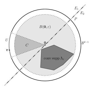
Figure 1. The sets defined in the proof of Proposition 3.11.

Example 3.12.

Suppose that $\boldsymbol{L}$ is a pure jump Lévy process with mutually independent, non-degenerate components $(L^{i}_{t})_{t\in\mathbb{R}}$, $i=1,\ldots,d$. Then the Lévy measure $\Lambda$ of $\boldsymbol{L}$ is concentrated on the coordinate axes of $\mathbb{R}^{d}$; see, e.g., [41, Exercise 12.10, p. 67]. More concretely, $\Lambda$ admits then a polar decomposition $\{\zeta,\rho_{\boldsymbol{u}}:\boldsymbol{u}\in\mathscr{S}^{d-1}\}$, with

$$\zeta=\sum_{i=1}^{d}(\delta_{\boldsymbol{e}_{i}}+\delta_{-\boldsymbol{e}_{i}}),$$

where $\delta_{\boldsymbol{x}}$ denotes the Dirac measure at $\boldsymbol{x}\in\mathbb{R}^{d}$ and $\boldsymbol{e}_{i}$ is the $i$-th canonical basis vector of $\mathbb{R}^{d}$, and for any $i=1,\ldots,d$ and $A\in\mathscr{B}(\mathbb{R}_{++})$,

$$\rho_{\boldsymbol{e}_{i}}(A)=\lambda_{i}(A)\quad\textrm{and}\quad\rho_{-\boldsymbol{e}_{i}}(A)=\lambda_{i}(-A),$$

where $\lambda_{i}$ denotes the the Lévy measure of the component $(L^{i}_{t})_{t\in\mathbb{R}}$.

Clearly, $\zeta$ satisfies the condition (i) of Proposition 3.11 and (ii) holds provided that the Lévy measure $\lambda_{i}$, for any $i=1,\ldots,d$, satisfies the condition (JUMPS₁), namely, $\lambda_{i}\big{(}(-\varepsilon,0)\big{)}>0$ and $\lambda_{i}\big{(}(0,\varepsilon)\big{)}>0$ for any $\varepsilon>0$.

Example 3.13.

It is well known that the Lévy process $\boldsymbol{L}$ is self-decomposable (see [41, Section 3.15] for the usual definition) if and only if its Lévy measure $\Lambda$ admits a polar decomposition $\{\zeta,\rho_{\boldsymbol{u}}:\boldsymbol{u}\in\mathscr{S}^{d-1}\}$, where

$$\rho_{\boldsymbol{u}}(\mathrm{d}r)=\frac{\mathscr{K}({\boldsymbol{u}},r)}{r}\mathrm{d}r,\quad\textrm{$\zeta$-almost every $\boldsymbol{u}\in\mathscr{S}^{d-1}$,}$$

for some function $\mathscr{K}:\mathscr{S}^{d-1}\times\mathbb{R}_{++}\rightarrow\mathbb{R}_{+}$ such that $\mathscr{K}({\boldsymbol{u}},r)$ is measurable in $\boldsymbol{u}$ and decreasing in $r$ [41, Theorem 15.10, p. 95]. For example, for $\alpha\in(0,2)$, setting $\mathscr{K}({\boldsymbol{u}},r)\mathrel{\mathop{:}}=r^{-\alpha}$ for all $\boldsymbol{u}\in\mathscr{S}^{d-1}$ and $r>0$, we recover the subclass of $\alpha$-stable processes [41, Theorem 14.3, pp. 77–78]. Clearly, the condition (ii) in Proposition 3.11 is then met if $\sup_{r>0}\mathscr{K}({\boldsymbol{u}},r)>0$ for $\zeta$-almost every $\boldsymbol{u}\in\mathscr{S}^{d-1}$.

3.3.2. Multivariate subordination

Subordination is a classical method of constructing a new Lévy process by time-changing an existing Lévy process with an independent subordinator, a Lévy process with non-decreasing trajectories; see, e.g., [41, Chapter 6]. Barndorff-Nielsen et al. [4] have introduced a multivariate extension of this technique, which, in particular, provides a way of constructing multivariate Lévy processes with dependent components (starting from Lévy processes whose components are mutually independent).

We discuss now, how the condition (JUMPS) can be checked when $\Lambda$ is the Lévy measure of a Lévy process $\boldsymbol{L}$ that has been constructed by multivariate subordination. For simplicity, we consider only a special case of the rather general framework introduced in [4]. As the key ingredient in multivariate subordination we take a family of $d\geqslant 2$ mutually independent, univariate Lévy processes $\big{(}\widetilde{L}^{i}_{t}\big{)}_{t\geqslant 0}$, $i=1,\ldots,d$, with respective triplets $\big{(}\tilde{b}_{i},0,\tilde{\lambda}_{i}\big{)}$, $i=1,\ldots,d$. (We eschew Gaussian parts here, as they would be irrelevant in the context of Theorem 2.9.) Additionally, we need a $d$-dimensional subordinator $(\boldsymbol{T}_{t})_{t\geqslant 0}$, independent of $\big{(}\widetilde{L}^{i}_{t}\big{)}_{t\geqslant 0}$, $i=1,\ldots,d$, which is a Lévy process whose triplet $(\boldsymbol{c},0,\rho)$ satisfies $\boldsymbol{c}=(c_{1},\ldots,c_{d})\in\mathbb{R}^{d}_{+}$ and $\operatorname{supp}\rho\subset\mathbb{R}^{d}_{+}$. We denote the components of $\boldsymbol{T}_{t}$ by $T^{1}_{t},\ldots,T^{d}_{t}$ for any $t\geqslant 0$.

By [4, Theorem 3.3], the time-changed process

$$\boldsymbol{L}_{t}\mathrel{\mathop{:}}=\Big{(}\widetilde{L}^{1}_{T^{1}_{t}},\ldots,\widetilde{L}^{d}_{T^{d}_{t}}\Big{)},\quad t\geqslant 0,$$ (3.18)

is a Lévy process with triplet $(\boldsymbol{b},0,\Lambda)$ given by

$$\boldsymbol{b} \mathrel{\mathop{:}}=\int_{\mathbb{R}_{+}^{d}}\rho(\mathrm{d}\boldsymbol{s})\int_{\{\|\boldsymbol{x}\|\leqslant 1\}}\boldsymbol{x}\mu_{\boldsymbol{s}}(\mathrm{d}\boldsymbol{x})+(c_{1}\tilde{b}_{1},\ldots,c_{d}\tilde{b}_{d}),$$

$$\Lambda(B) \mathrel{\mathop{:}}=\int_{\mathbb{R}_{+}^{d}}\mu_{\boldsymbol{s}}(B)\rho(\mathrm{d}\boldsymbol{s})+\int_{B}\big{(}c_{1}\mathbf{1}_{\mathscr{A}_{1}}(\boldsymbol{x})\tilde{\lambda}_{1}(\mathrm{d}x_{1})+\cdots+c_{d}\mathbf{1}_{\mathscr{A}_{d}}(\boldsymbol{x})\tilde{\lambda}_{d}(\mathrm{d}x_{d})\big{)},\,\,B\in\mathscr{B}(\mathbb{R}^{d}),$$ (3.19)

where

$$\mu_{\boldsymbol{s}}(\mathrm{d}\boldsymbol{x})\mathrel{\mathop{:}}=\mathbf{P}\Big{[}\widetilde{L}^{1}_{s_{1}}\in\mathrm{d}x_{1},\ldots,\widetilde{L}^{d}_{s_{d}}\in\mathrm{d}x_{d}\Big{]}=\prod_{j=1}^{d}\mathbf{P}\Big{[}\widetilde{L}^{j}_{s_{j}}\in\mathrm{d}x_{j}\Big{]},\quad\boldsymbol{s}\in\mathbb{R}_{+}^{d},$$

and $\mathscr{A}_{i}\mathrel{\mathop{:}}=\{\boldsymbol{x}\in\mathbb{R}^{d}:x_{j}=0,\,j\neq i\}$ is the $i$-th coordinate axis for any $i=1,\ldots,d$. (While (3.18) defines only a one-sided process $\boldsymbol{L}$, it can obviously be extended to a two-sided Lévy process using the construction (2.2).)

Proposition 3.14 (Multivariate subordination).

Suppose that the Lévy measure $\Lambda$ is given by (3.19) and that

$$\tilde{\lambda}_{i}\big{(}(-\varepsilon,0)\big{)}>0\quad\textrm{and}\quad\tilde{\lambda}_{i}\big{(}(0,\varepsilon)\big{)}>0\quad\textrm{for any $i=1,\ldots,d$ and $\varepsilon>0$.}$$ (3.20)

If $\boldsymbol{c}\in\mathbb{R}^{d}_{++}$ or $\mathbb{R}^{d}_{++}\cap\operatorname{supp}\rho=\varnothing$, then $\Lambda$ satisfies (JUMPS).

Proof.

Let $\boldsymbol{i}=(i_{1},\ldots,i_{d})\in\{0,1\}^{d}$, $\varepsilon>0$, and $B=B_{1}\times\cdots\times B_{d}\subset B(\boldsymbol{0},\varepsilon)$, where

$$B_{j}\mathrel{\mathop{:}}=\begin{cases}\big{(}0,\frac{\varepsilon}{\sqrt{d}}\big{)},&i_{j}=1,\\ \big{(}-\frac{\varepsilon}{\sqrt{d}},0\big{)},&i_{j}=0,\\ \end{cases}$$

for any $j=1,\ldots,d$. We observe that

$$\Lambda_{\varepsilon}(B)=\Lambda(B)\geqslant\int_{B}\big{(}c_{1}\mathbf{1}_{\mathscr{A}_{1}}(\boldsymbol{x})\tilde{\lambda}_{1}(\mathrm{d}x_{1})+\cdots+c_{d}\mathbf{1}_{\mathscr{A}_{d}}(\boldsymbol{x})\tilde{\lambda}_{d}(\mathrm{d}x_{d})\big{)}=\sum_{i=1}^{d}c_{i}\tilde{\lambda}(B_{i})>0,$$ (3.21)

when $\boldsymbol{c}\in\mathbb{R}^{d}_{++}$. The assumption (3.20) implies, by Lemma 4.5 below, that $\operatorname{supp}\mu_{\boldsymbol{s}}=\mathbb{R}^{d}$, and consequently $\mu_{\boldsymbol{s}}(B)>0$, for any $\boldsymbol{s}\in\mathbb{R}^{d}_{++}$. Thus,

$$\Lambda_{\varepsilon}(B)=\Lambda(B)\geqslant\int_{\mathbb{R}_{++}^{d}}\mu_{\boldsymbol{s}}(B)\rho(\mathrm{d}\boldsymbol{s})>0,$$ (3.22)

when $\mathbb{R}^{d}_{++}\cap\operatorname{supp}\rho=\varnothing$. It follows from (3.21) and (3.22), that $\operatorname{supp}\Lambda_{\varepsilon}$ intersects with any open orthant of $\mathbb{R}^{d}$, which in turn implies that $\Lambda$ satisfies (JUMPS). ∎

3.3.3. Lévy copulas

Let $d\geqslant 2$. The Lévy measure $\Lambda$ on $\mathbb{R}^{d}$ can be defined by specifying $d$ one-dimensional marginal Lévy measures and describing the dependence structure through a Lévy copula, a concept introduced by Kallsen and Tankov [28]. We provide first a very brief introduction to Lévy copulas, following [28].

Below, $\overline{\mathbb{R}}\mathrel{\mathop{:}}=(-\infty,\infty]$. Moreover, for $\boldsymbol{a}=(a_{1},\ldots,a_{d}),\,\boldsymbol{b}=(b_{1},\ldots,b_{d})\in\overline{\mathbb{R}}^{d}$, we write $\boldsymbol{a}\leqslant\boldsymbol{b}$ (resp. $\boldsymbol{a}<\boldsymbol{b}$) if $a_{i}\leqslant b_{i}$ (resp. $a_{i}<b_{i}$) for any $i=1,\ldots,d$. For any $\boldsymbol{a}\leqslant\boldsymbol{b}$ we denote by $(\boldsymbol{a},\boldsymbol{b}]$ the hyperrectangle $\prod_{i=1}^{d}(a_{i},b_{i}]$.

Definition 3.15.

Let $F:\overline{\mathbb{R}}^{d}\rightarrow\overline{\mathbb{R}}^{d}$ and let $\boldsymbol{a},\,\boldsymbol{b}\in\overline{\mathbb{R}}^{d}$ be such that $\boldsymbol{a}\leqslant\boldsymbol{b}$. The rectangular increment of $F$ over the hyperrectangle $(\boldsymbol{a},\boldsymbol{b}]\subset\overline{\mathbb{R}}^{d}$ is defined by

$$F\big{(}(\boldsymbol{a},\boldsymbol{b}]\big{)}\mathrel{\mathop{:}}=\sum_{\boldsymbol{i}\in\{0,1\}^{d}}(-1)^{d-\sum_{j=1}^{d}i_{j}}F\big{(}(1-i_{1})a_{1}+i_{1}b_{1},\ldots,(1-i_{d})a_{d}+i_{d}b_{d}\big{)}.$$

We say that $F$ is $d$-increasing if $F\big{(}(\boldsymbol{a},\boldsymbol{b}]\big{)}\geqslant 0$ for any $\boldsymbol{a},\,\boldsymbol{b}\in\overline{\mathbb{R}}^{d}$ such that $\boldsymbol{a}\leqslant\boldsymbol{b}$. Further, we say that $F$ is strictly $d$-increasing if $F\big{(}(\boldsymbol{a},\boldsymbol{b}]\big{)}>0$ for any $\boldsymbol{a},\,\boldsymbol{b}\in\overline{\mathbb{R}}^{d}$ such that $\boldsymbol{a}<\boldsymbol{b}$.

Definition 3.16.

Let $F:\overline{\mathbb{R}}^{d}\rightarrow\overline{\mathbb{R}}^{d}$ be $d$-increasing, with $F(x_{1},\ldots,x_{d})=0$ whenever $x_{i}=0$ for some $i=1,\ldots,d$. For any non-empty $I\subset\{1,\ldots,d\}$, the $I$-margin of $F$ is a function $F^{I}:\overline{\mathbb{R}}^{|I|}\rightarrow\overline{\mathbb{R}}$ given by

$$F^{I}\big{(}(x_{i})_{i\in I}\big{)}\mathrel{\mathop{:}}=\lim_{u\rightarrow-\infty}\sum_{(x_{i})_{i\in I^{c}}\in\{u,\infty\}^{|I^{c}|}}F(x_{1},\ldots,x_{d})\prod_{i\in I^{c}}\mathrm{sgn}(x_{i}),$$

where $\mathrm{sgn}(x)\mathrel{\mathop{:}}=-\mathbf{1}_{(-\infty,0)}(x)+\mathbf{1}_{[0,\infty)}(x)$, $x\in\mathbb{R}$, and $I^{c}$ stands for the complement $\{1,\ldots,d\}\setminus I$.

Definition 3.17.

A $d$-dimensional Lévy copula is a function $C:\overline{\mathbb{R}}^{d}\rightarrow\overline{\mathbb{R}}$ such that

1. $C(x_{1}\ldots,x_{d})<\infty$ when $x_{i}<\infty$ for all $i=1\ldots,d$,

2. $C(x_{1}\ldots,x_{d})=0$ when $x_{i}=0$ for some $i=1\ldots,d$,

3. $C$ is $d$-increasing,

4. $C^{\{i\}}(x)=x$ for all $x\in\mathbb{R}$ and $i=1\ldots,d$.

Remark 3.18.

The properties (ii), (iii), and (iv) of a Lévy copula are analogous to the defining properties of a classical copula; see, e.g., [34, Definition 2.10.6].

Recall that a classical copula describes a probability measure on $\mathbb{R}^{d}$ through its cumulative distribution function, by Sklar’s theorem [34, Theorem 2.10.9]. In the context of Lévy copulas, the cumulative distribution function is replaced with the tail integral of the Lévy measure, which is defined as follows.

Definition 3.19.

The tail integral of the Lévy measure $\Lambda$ is a function $J_{\Lambda}:(\mathbb{R}\setminus\{0\})^{d}\rightarrow\mathbb{R}$ given by

$$J_{\Lambda}(x_{1},\ldots,x_{d})\mathrel{\mathop{:}}=\Lambda\bigg{(}\prod_{j=1}^{d}\mathscr{I}(x_{j})\bigg{)}\prod_{i=1}^{d}\mathrm{sgn}(x_{i}),$$

where

$$\mathscr{I}(x)\mathrel{\mathop{:}}=\begin{cases}(x,\infty),&x\geqslant 0,\\ (-\infty,x],&x<0.\end{cases}$$

Definition 3.20.

Let $I\subset\{1,\ldots,d\}$ be non-empty. The $I$-marginal tail integral of the Lévy measure $\Lambda$, denoted by $J^{I}_{\Lambda}$, is the tail integral of the Lévy measure $\Lambda^{I}$ of the process $\boldsymbol{L}^{I}\mathrel{\mathop{:}}=(L^{i})_{i\in I}$, which consists of components of the Lévy process $\boldsymbol{L}$ with Lévy measure $\Lambda$.

Kallsen and Tankov [28, Lemma 3.5] have shown that the Lévy measure $\Lambda$ is fully determined by its marginal tail integrals $J^{I}_{\Lambda}$, $I\subset\{1,\ldots,d\}$ is non-empty. Moreover, they have proved a Sklar’s theorem for Lévy copulas [28, Theorem 3.6], which says that for any Lévy measure $\Lambda$ on $\mathbb{R}^{d}$, there exists a Lévy copula $C$ that satisfies

$$J^{I}_{\Lambda}\big{(}(x_{i})_{i\in I}\big{)}=C^{I}\Big{(}\big{(}J_{\Lambda}^{\{i\}}(x_{i})\big{)}_{i\in I}\Big{)}$$

for any non-empty $I\subset\{1,\ldots,d\}$ and any $(x_{i})_{i\in I}\in(\mathbb{R}\setminus\{0\})^{|I|}$. Conversely, we can construct $\Lambda$ from a Lévy copula $C$ and (one-dimensional) marginal Lévy measures $\lambda_{i}$, $i=1,\ldots,d$, by defining

$$J^{I}_{\Lambda}\big{(}(x_{i})_{i\in I}\big{)}\mathrel{\mathop{:}}=C^{I}\Big{(}\big{(}J_{\lambda_{i}}(x_{i})\big{)}_{i\in I}\Big{)}$$

for any non-empty $I\subset\{1,\ldots,d\}$ and any $(x_{i})_{i\in I}\in(\mathbb{R}\setminus\{0\})^{|I|}$. Then we say that $\Lambda$ has Lévy copula $C$ and marginal Lévy measures $\lambda_{i}$, $i=1,\ldots,d$.

We can now show that $\Lambda$ satisfies (JUMPS) if it has strictly $d$-increasing Lévy copula and marginal Lévy measures such that each of them satisfies (JUMPS₁).

Proposition 3.21 (Lévy copula).

Suppose that the Lévy measure $\Lambda$ has Lévy copula $C$ and marginal Lévy measures $\lambda_{i}$, $i=1,\ldots,d$. If

1. $C$ is strictly $d$-increasing,

2. $\lambda_{i}\big{(}(-\varepsilon,0)\big{)}>0$ and $\lambda_{i}\big{(}(0,\varepsilon)\big{)}>0$ for any $i=1,\ldots,d$ and $\varepsilon>0$,

then $\Lambda$ satisfies (JUMPS).

Remark 3.22.

Proposition 3.21 has the caveat that its assumptions do not cover the case where $\Lambda$ is the Lévy measure of a Lévy process with independent components, discussed in Example 3.12. Indeed, the corresponding “independence Lévy copula”, characterized in [28, Proposition 4.1], is not strictly $d$-increasing. However, it is worth pointing out that it is not sufficient in Proposition 3.21 that $C$ is merely $d$-increasing, as this requirement is met by all Lévy copulas, including those that give rise to Lévy processes with perfectly dependent components; see, e.g., [28, Theorem 4.4].

Proof of Proposition 3.21.

Let $\boldsymbol{a},\,\boldsymbol{b}\in\overline{\mathbb{R}}^{d}$ be such that $\boldsymbol{a}\leqslant\boldsymbol{b}$ and $a_{i}b_{i}>0$ for any $i=1,\ldots,d$. Then

$$J_{\Lambda}((\boldsymbol{a},\boldsymbol{b}])=\sum_{\boldsymbol{i}\in\{0,1\}^{d}}(-1)^{d-\sum_{j=1}^{d}i_{j}}J_{\Lambda}\big{(}(1-i_{1})a_{1}+i_{1}b_{1},\ldots,(1-i_{d})a_{d}+i_{d}b_{d}\big{)},$$ (3.23)

where

$$J_{\Lambda}\big{(}(1-i_{1})a_{1}+i_{1}b_{1},\ldots,(1-i_{d})a_{d}+i_{d}b_{d}\big{)}\\ \begin{aligned} &=C\big{(}J_{\lambda_{1}}\big{(}(1-i_{1})a_{1}+i_{1}b_{1}\big{)},\ldots,J_{\lambda_{d}}\big{(}(1-i_{d})a_{d}+i_{d}b_{d}\big{)}\big{)}\\ &=C\big{(}i_{1}J_{\lambda_{1}}(b_{1})+(1-i_{1})J_{\lambda_{1}}(a_{1}),\ldots,i_{d}J_{\lambda_{d}}(b_{d})+(1-i_{d})J_{\lambda_{d}}(a_{d})\big{)}.\end{aligned}$$ (3.24)

It follows from Definition 3.19 that $x\mapsto J_{\lambda_{i}}(x)$ is non-increasing on the intervals $(-\infty,0)$ and $(0,\infty)$ for any $i=1,\ldots,d$. Thus,

$$\tilde{\boldsymbol{b}}\mathrel{\mathop{:}}=\big{(}J_{\lambda_{1}}(b_{1}),\ldots,J_{\lambda_{d}}(b_{d})\big{)}\leqslant\big{(}J_{\lambda_{1}}(a_{1}),\ldots,J_{\lambda_{d}}(a_{d})\big{)}=\mathrel{\mathop{:}}\tilde{\boldsymbol{a}}.$$ (3.25)

Furthermore, by (3.23) and (3.24),

$$(-1)^{d}J_{\nu}((\boldsymbol{a},\boldsymbol{b}])=C\big{(}(\tilde{\boldsymbol{b}},\tilde{\boldsymbol{a}}]\big{)}.$$

We establish (JUMPS) by showing that the intersection of each open orthant of $\mathbb{R}^{d}$ with $\operatorname{supp}\Lambda_{\varepsilon}$ is non-empty for any $\varepsilon>0$. To this end, let $\varepsilon>0$, $n\in\mathbb{N}$, and $\boldsymbol{i}\in\{0,1\}^{d}$. Define $\boldsymbol{a},\,\boldsymbol{b}\in\mathbb{R}^{d}$ by

$$\boldsymbol{a} \mathrel{\mathop{:}}=\frac{\varepsilon}{\sqrt{d+1}}\bigg{(}\frac{i_{1}}{n}-(1-i_{1}),\ldots,\frac{i_{d}}{n}-(1-i_{d})\bigg{)},$$

$$\boldsymbol{b} \mathrel{\mathop{:}}=\frac{\varepsilon}{\sqrt{d+1}}\bigg{(}i_{1}-\frac{1-i_{1}}{n},\ldots,i_{d}-\frac{1-i_{d}}{n}\bigg{)}.$$

Note that $\boldsymbol{a}\leqslant\boldsymbol{b}$ and that $(\boldsymbol{a},\boldsymbol{b}]\subset B(\boldsymbol{0},\varepsilon)$. Moreover, $(\boldsymbol{a},\boldsymbol{b}]$ belongs to the open orthant

$$\{(x_{1},\ldots,x_{d})\in\mathbb{R}^{d}:(-1)^{1-i_{j}}x_{j}>0,\,j=1,\ldots,d\},$$

It suffices now to show that $\Lambda((\boldsymbol{a},\boldsymbol{b}])>0$ for some $n\in\mathbb{N}$. Since $a_{i}b_{i}>0$ for any $i=1,\ldots,d$, we have (cf. the proof of [28, Lemma 3.5])

$$\Lambda((\boldsymbol{a},\boldsymbol{b}])=(-1)^{d}J_{\Lambda}((\boldsymbol{a},\boldsymbol{b}])=C\big{(}(\tilde{\boldsymbol{b}},\tilde{\boldsymbol{a}}]\big{)},$$

where $\tilde{\boldsymbol{a}}$ and $\tilde{\boldsymbol{b}}$ are derived from $\boldsymbol{a}$ and $\boldsymbol{b}$ via (3.25). Observe that for any $j=1,\ldots,d$,

$$\tilde{a}_{j}-\tilde{b}_{j}=J_{\lambda_{j}}(a_{j})-J_{\lambda_{j}}(b_{j})=\begin{cases}\lambda_{j}\big{(}\big{(}\frac{\varepsilon}{n\sqrt{d+1}},\frac{\varepsilon}{\sqrt{d+1}}\big{]}\big{)},&i_{j}=1,\\ \lambda_{j}\big{(}\big{(}\frac{-\varepsilon}{\sqrt{d+1}},\frac{-\varepsilon}{n\sqrt{d+1}}\big{]}\big{)},&i_{j}=0.\end{cases}$$

It follows now from the assumption (ii) that for some sufficiently large $n\geq 2$, we have $\tilde{b}_{j}<\tilde{a}_{j}$ for any $j=1,\ldots,d$, that is, $\tilde{\boldsymbol{b}}<\tilde{\boldsymbol{a}}$. Thanks to the assumption (i), we can then conclude that $\Lambda((\boldsymbol{a},\boldsymbol{b}])=C\big{(}(\tilde{\boldsymbol{b}},\tilde{\boldsymbol{a}}]\big{)}>0$. ∎

Example 3.23.

We provide here a simple example of a $d$-strictly increasing Lévy copula, following the construction — which parallels that of Archimedean copulas [34, Chapter 4] in the classical setting — given by Kallsen and Tankov [28, Theorem 6.1]. Suppose that $\varphi:[-1,1]\rightarrow[-\infty,\infty]$ is some strictly increasing continuous function such that $\varphi(1)=\infty$, $\varphi(0)=0$, and $\varphi(-1)=-\infty$. Assume, moreover, that $\varphi$ is $d$ times differentiable on $(-1,0)$ and $(0,1)$, so that

$$\frac{\mathrm{d}^{d}\varphi(e^{x})}{\mathrm{d}x^{d}}>0\quad\textrm{and}\quad\frac{\mathrm{d}^{d}\varphi(-e^{x})}{\mathrm{d}x^{d}}<0\quad\textrm{for any $x\in(-\infty,0)$.}$$ (3.26)

In [28, Theorem 6.1] it has been shown that the function

$$C(x_{1},\ldots,x_{d})\mathrel{\mathop{:}}=\varphi\Bigg{(}\prod_{i=1}^{d}\tilde{\varphi}^{-1}(x_{i})\Bigg{)},\quad(x_{1},\ldots,x_{d})\in\overline{\mathbb{R}}^{d},$$

where $\tilde{\varphi}(x)\mathrel{\mathop{:}}=2^{d-2}\big{(}\varphi(x)-\varphi(-x)\big{)}$, $x\in[-1,1]$, is a Lévy copula. (In fact, in [28] the Lévy copula property is shown under weaker assumptions with non-strict inequalities in (3.26).) The argument used in the proof of [28, Theorem 6.1] to show that $C$ is $d$-increasing translates easily to a proof that $C$ is also strictly $d$-increasing under (3.26). One can take, e.g., $\varphi(x)\mathrel{\mathop{:}}=\frac{x}{1-|x|}$, $x\in[-1,1]$, which satisfies the conditions above. In particular,

$$\frac{\mathrm{d}^{d}\varphi(x)}{\mathrm{d}x^{d}} =\frac{d!}{(1-x)^{d+1}}>0,\quad x\in(0,1),$$

$$(-1)^{d}\frac{\mathrm{d}^{d}\varphi(x)}{\mathrm{d}x^{d}} =-\frac{d!}{(1+x)^{d+1}}<0,\quad x\in(-1,0),$$

which ensure that (3.26) holds.

3.3.4. Lévy mixing

It is also possible to define new Lévy measures on $\mathbb{R}^{d}$, for $d\geqslant 2$, by mixing suitable transformations of a given Lévy measure on $\mathbb{R}^{d}$ — a technique that is called Lévy mixing. We focus here on a particular type of Lévy mixing, the so-called Upsilon transformation, introduced by Barndorff-Nielsen et al. [5] in the multivariate setting.

The Upsilon transformation amounts to mixing linear transformations of a Lévy measure on $\mathbb{R}^{d}$. To state the definition of the Upsilon transformation, let $(S,\mathscr{S},\rho)$ be a $\sigma$-finite measure space that parametrizes a family of linear transformations $\mathbb{R}^{d}\rightarrow\mathbb{R}^{d}$ via a measurable function $A:S\rightarrow\mathbb{M}_{d}$. The Upsilon transformation of a Lévy measure $\Gamma$ on $\mathbb{R}^{d}$ under $A$, denoted $\Upsilon^{0}_{A}[\Gamma]$, is then a Borel measure on $\mathbb{R}^{d}$ defined by

$$\Upsilon^{0}_{A}[\Gamma](B)\mathrel{\mathop{:}}=\int_{S}\int_{\mathbb{R}^{d}}\mathbf{1}_{B\setminus\{\boldsymbol{0}\}}(A(s)\boldsymbol{x})\Gamma(\mathrm{d}\boldsymbol{x})\rho(\mathrm{d}s),\quad B\in\mathscr{B}(\mathbb{R}^{d}).$$

Barndorff-Nielsen et al. [5, Theorem 3.3] have shown that the Upsilon transformation $\Upsilon^{0}_{A}$ maps Lévy measures to Lévy measures, a crucial property for the validity of this approach, if and only if

$$\rho(\{s\in S:A(s)\neq 0\})<\infty,\quad\int_{S}\|A(s)\|^{2}\rho(\mathrm{d}s)<\infty.$$ (3.27)

We show here that the Upsilon transformation preserves the property (JUMPS), provided that the function $A$ has a natural non-degeneracy property: the matrix $A(s)$ is invertible for any $s$ in a set with positive $\rho$-measure. This result can be applied to construct multivariate Lévy processes with dependent components for example by applying the Upsilon transformation to the Lévy measure of a Lévy process with independent components, which satisfies (JUMPS) under mild conditions that are easy to check; see Example 3.12.

Proposition 3.24 (Upsilon transformation).

Let $(S,\mathscr{S},\rho)$ be a $\sigma$-finite measure space and let $A:(S,\mathscr{S})\rightarrow\mathbb{M}_{d}$ be measurable function such that (3.27) holds and

$$\rho(\{s\in S:\det(A(s))\neq 0\})>0.$$

Moreover, let $\Gamma$ be a Lévy measure on $\mathbb{R}^{d}$ that satisfies (JUMPS). Then the Upsilon transformation $\Lambda\mathrel{\mathop{:}}=\Upsilon^{0}_{A}[\Gamma]$ defines a Lévy measure satisfying (JUMPS).

Proof.

Suppose that $\Lambda=\Upsilon^{0}_{A}[\Gamma]$ does not satisfy (JUMPS). Then, adapting the early steps seen in the proof of Proposition 3.11, we may find an open half-ball $H(\boldsymbol{c},\varepsilon)\mathrel{\mathop{:}}=\{\boldsymbol{x}\in\mathbb{R}^{d}:\langle\boldsymbol{x},\boldsymbol{c}\rangle>0,\,\|\boldsymbol{x}\|<\varepsilon\}$, for some $\boldsymbol{c}\in\mathbb{R}^{d}\setminus\{\boldsymbol{0}\}$ and $\varepsilon>0$, such that $\Lambda\big{(}H(\boldsymbol{c},\varepsilon)\big{)}=0$.

Assume for now that $s\in S_{A}\mathrel{\mathop{:}}=\{s\in S:\det(A(s))\neq 0\}$. Then $\|A(s)\boldsymbol{x}\|\leqslant\|A(s)\|\|\boldsymbol{x}\|$ for any $\boldsymbol{x}\in\mathbb{R}^{d}$, where $\|A(s)\|>0$. So we can deduce that if

$$\boldsymbol{x}\in H\bigg{(}A(s)^{\top}\boldsymbol{c},\frac{\varepsilon}{\|A(s)\|}\bigg{)}=\bigg{\{}\boldsymbol{x}\in\mathbb{R}^{d}:\langle\boldsymbol{x},A(s)^{\top}\boldsymbol{c}\rangle>0,\,\|\boldsymbol{x}\|<\frac{\varepsilon}{\|A(s)\|}\bigg{\}},$$

then $A(s)\boldsymbol{x}\in H(\boldsymbol{c},\varepsilon)$. Observe also that $H\big{(}A(s)^{\top}\boldsymbol{c},\frac{\varepsilon}{\|A(s)\|}\big{)}$ is an open half-ball since $A(s)^{\top}\boldsymbol{c}\in\mathbb{R}^{d}\setminus\{\boldsymbol{0}\}$, due to the property $\det(A(s)^{\top})=\det(A(s))\neq 0$.

Noting that $\boldsymbol{0}\notin H(\boldsymbol{c},\varepsilon)$, we have thus

$$\begin{split}0=\Lambda\big{(}H(\boldsymbol{c},\varepsilon)\big{)}=\Upsilon^{0}_{A}[\Gamma]\big{(}H(\boldsymbol{c},\varepsilon)\big{)}&=\int_{S}\int_{\mathbb{R}^{d}}\mathbf{1}_{H(\boldsymbol{c},\varepsilon)\setminus\{\boldsymbol{0}\}}(A(s)\boldsymbol{x})\Gamma(\mathrm{d}\boldsymbol{x})\rho(\mathrm{d}s)\\ &\geqslant\int_{S_{A}}\int_{\mathbb{R}^{d}}\mathbf{1}_{H(\boldsymbol{c},\varepsilon)}(A(s)\boldsymbol{x})\Gamma(\mathrm{d}\boldsymbol{x})\rho(\mathrm{d}s)\\ &\geqslant\int_{S_{A}}\Gamma\Bigg{(}H\bigg{(}A(s)^{\top}\boldsymbol{c},\frac{\varepsilon}{\|A(s)\|}\bigg{)}\Bigg{)}\rho(\mathrm{d}s).\end{split}$$ (3.28)

Now for any $s\in S_{A}$, the open half-ball $H\big{(}A(s)^{\top}\boldsymbol{c},\frac{\varepsilon}{\|A(s)\|}\big{)}$ has positive $\Gamma$-measure since $\Gamma$ satisfies (JUMPS). But $\rho(S_{A})>0$, by assumption, so in view of (3.28) we have a contradiction. ∎

4. Proofs of the main results

4.1. Proof of Theorem 2.7

The proof of the CFS property in the Gaussian case follows the strategy used by Cherny [20], but adapts it to a multivariate setting.

We start with a multivariate extension of a result [20, Lemma 2.1] regarding density of convolutions. The proof of [20, Lemma 2.1] is based on Titchmarsh’s convolution theorem (see Lemma A.1 in Appendix A), whereas we use a multivariate extension of Titchmarsh’s convolution theorem (Lemma A.2 in Appendix A), which is due to Kalisch [26], to prove the following result.

Lemma 4.1.

Let $\Phi=[\Phi_{i,j}]_{i,j\in\{1,\ldots,d\}^{2}}\in L^{2}_{\mathrm{loc}}(\mathbb{R}_{+},\mathbb{M}_{d})$ satisfy (DET-*) and let $0\leqslant t_{0}<T<\infty$. Then the linear operator $T_{\Phi}:L^{2}([t_{0},T],\mathbb{R}^{d})\rightarrow C_{\boldsymbol{0}}([t_{0},T],\mathbb{R}^{d})$, given by

$$(T_{\Phi}\boldsymbol{f})(t)\mathrel{\mathop{:}}=\int_{t_{0}}^{t}\Phi(t-s)\boldsymbol{f}(s)\mathrm{d}s,\quad t\in[t_{0},T],\quad\boldsymbol{f}\in L^{2}([t_{0},T],\mathbb{R}^{d}),$$

has dense range.

Proof.

By a change of variable, we may assume that $t_{0}=0$, in which case $T_{\Phi}\boldsymbol{f}=\Phi*\boldsymbol{f}$. Analogously to the proof of [20, Lemma 2.1], it suffices to show that the range of $T_{\Phi}$, denoted $\operatorname{ran}T_{\Phi}$, is dense in $L^{2}([0,T],\mathbb{R}^{d})$.

Suppose that, instead, $\operatorname{cl}\operatorname{ran}T_{\Phi}$, is a strict subset of $L^{2}([0,T],\mathbb{R}^{d})$. Since $\operatorname{cl}\operatorname{ran}T_{\Phi}$ is a closed linear subspace of $L^{2}([0,T],\mathbb{R}^{d})$, its orthogonal complement $(\operatorname{cl}\operatorname{ran}T_{\Phi})^{\perp}$ is non-trivial. Thus, there exist $\boldsymbol{h}=(h_{1},\ldots,h_{d})\in(\operatorname{cl}\operatorname{ran}T_{\Phi})^{\perp}$ such that

$$\operatorname{ess\,supp}\boldsymbol{h}\neq\varnothing.$$ (4.1)

Take arbitrary $\boldsymbol{f}=(f_{1},\ldots,f_{d})\in L^{2}([0,T],\mathbb{R}^{d})$. On the one hand, using Fubini’s theorem and substitutions $u\mathrel{\mathop{:}}=T-s$ and $v\mathrel{\mathop{:}}=T-t$, we get

$$\begin{split}\int_{0}^{T}\langle(\Phi*\boldsymbol{f})(t),\boldsymbol{h}(t)\rangle\mathrm{d}t&=\int_{0}^{T}\sum_{i=1}^{n}\bigg{(}\sum_{j=1}^{n}\int_{0}^{t}\Phi_{i,j}(t-s)f_{j}(s)\mathrm{d}s\bigg{)}h_{i}(t)\mathrm{d}t\\ &=\int_{0}^{T}\sum_{j=1}^{n}f_{j}(T-u)\bigg{(}\sum_{i=1}^{n}\int_{0}^{u}\Phi_{i,j}(u-v)h_{i}(T-v)\mathrm{d}v\bigg{)}\mathrm{d}u\\ &=\int_{0}^{T}\langle\boldsymbol{f}(T-u),(\Phi^{\top}*\boldsymbol{h}(T-\cdot))(u)\rangle\mathrm{d}u.\end{split}$$

On the other hand, as $\boldsymbol{h}\in(\operatorname{cl}\operatorname{ran}T_{\Phi})^{\perp}$,

$$\int_{0}^{T}\langle(\Phi*\boldsymbol{f})(t),\boldsymbol{h}(t)\rangle\mathrm{d}t=\boldsymbol{0}.$$

Thus, $(\Phi^{\top}*\boldsymbol{h}(T-\cdot))(u)=\mathbf{0}$ for almost all $u\in[0,T]$. Since $\mathrm{det}^{*}(\Phi^{\top})=\mathrm{det}^{*}(\Phi)$, by Lemma A.3(ii), it follows from Lemma A.2 that $\boldsymbol{h}(T-t)=\boldsymbol{0}$ for almost all $t\in[0,T]$, contradicting (4.1). ∎

Next we prove a small, but important, result that enables us to deduce the conclusion of Theorem 2.7 by establishing an unconditional small ball property for the auxiliary process $\bar{\boldsymbol{X}}^{t_{0}}$ for any $t_{0}\in[0,T)$. Here, neither Gaussianity nor continuity of $\boldsymbol{X}$ is assumed as the result will also be used later in the proof of Theorem 2.9. We remark that a similar result, albeit less general, is essentially embedded in the argument that appears in the proof of [20, Theorem 1.1].

Lemma 4.2.

Let $T>0$. Suppose that $\boldsymbol{X}$ is càdlàg and $\boldsymbol{A}^{t_{0}}$ is continuous for any $t_{0}\in[0,T)$. If

$$\mathbf{P}\bigg{[}\sup_{t\in[t_{0},T]}\big{\|}\bar{\boldsymbol{X}}^{t_{0}}_{t}-\boldsymbol{f}(t)\big{\|}<\varepsilon\bigg{]}>0\quad\textrm{for any $t_{0}\in[0,T)$, $\boldsymbol{f}\in C_{\boldsymbol{0}}([t_{0},T],\mathbb{R}^{d})$ and $\varepsilon>0$,}$$ (4.2)

then $(\boldsymbol{X}_{t})_{t\in[0,T]}$ has the CSBP with respect to $\big{(}\mathscr{F}^{\boldsymbol{L},\mathrm{inc}}_{t}\big{)}_{t\in[0,T]}$.

Proof.

By construction, $(\boldsymbol{X}_{t})_{t\in[0,T]}$ is adapted to $\big{(}\mathscr{F}^{\boldsymbol{L},\mathrm{inc}}_{t}\big{)}_{t\in[0,T]}$. We have, by (2.8), for any $t_{0}\in[0,T)$, $\boldsymbol{f}\in C_{\boldsymbol{0}}([t_{0},T],\mathbb{R}^{d})$, and $\varepsilon>0$,

$$\begin{split}\mathbf{P}\bigg{[}\sup_{t\in[t_{0},T]}\|\boldsymbol{X}_{t}-\boldsymbol{X}_{t_{0}}-\boldsymbol{f}(t)\|<\varepsilon\,\bigg{|}\,\mathscr{F}_{t_{0}}\bigg{]}&=\mathbf{P}\bigg{[}\sup_{t\in[t_{0},T]}\big{\|}\bar{\boldsymbol{X}}^{t_{0}}_{t}+\mathbf{A}^{t_{0}}_{t}-\boldsymbol{f}(t)\big{\|}<\varepsilon\,\bigg{|}\,\mathscr{F}_{t_{0}}\bigg{]}\\ &=\mathbf{E}\big{[}U\big{(}\bar{\boldsymbol{X}}^{t_{0}},\boldsymbol{f}-\mathbf{A}^{t_{0}}\big{)}\big{|}\mathscr{F}_{t_{0}}\big{]},\end{split}$$ (4.3)

where

$$U(\boldsymbol{g},\boldsymbol{h})\mathrel{\mathop{:}}=\mathbf{1}_{\{\sup_{t\in[t_{0},T]}\|\boldsymbol{g}(t)-\boldsymbol{h}(t)\|<\varepsilon\}},\quad\boldsymbol{g}\in D([t_{0},T],\mathbb{R}^{d}),\quad\boldsymbol{h}\in C([t_{0},T],\mathbb{R}^{d}).$$

(Note that $\bar{\boldsymbol{X}}^{t_{0}}$ is càdlàg since $\boldsymbol{X}$ is càdlàg and $\boldsymbol{A}^{t_{0}}$ is continuous.) The space $D([t_{0},T],\mathbb{R}^{d})$ is Polish, so the random element $\bar{\boldsymbol{X}}^{t_{0}}$ in $D([t_{0},T],\mathbb{R}^{d})$ has a regular conditional law given $\mathscr{F}_{t_{0}}^{\boldsymbol{L},\mathrm{inc}}$. However, as $\bar{\boldsymbol{X}}^{t_{0}}$ is independent of $\mathscr{F}_{t_{0}}^{\boldsymbol{L},\mathrm{inc}}$, this conditional law coincides almost surely with the unconditional law $\mathbf{P}\big{[}\bar{\boldsymbol{X}}^{t_{0}}\in\mathrm{d}\boldsymbol{x}\big{]}$. By the $\mathscr{F}_{t_{0}}^{\boldsymbol{L},\mathrm{inc}}$-measurability of the random element $\mathbf{A}^{t_{0}}$, the disintegration formula [27, Theorem 6.4] yields

$$\mathbf{E}\big{[}U\big{(}\bar{\boldsymbol{X}}^{t_{0}},\boldsymbol{f}-\mathbf{A}^{t_{0}}\big{)}\big{|}\mathscr{F}_{t_{0}}\big{]}=\int_{D([t_{0},T],\mathbb{R}^{d})}U\big{(}\boldsymbol{x},\boldsymbol{f}-\mathbf{A}^{t_{0}}\big{)}\mathbf{P}\big{[}\bar{\boldsymbol{X}}^{t_{0}}\in\mathrm{d}\boldsymbol{x}\big{]}\quad\textrm{almost surely.}$$

Evidently,

$$\mathbf{P}\bigg{[}\sup_{t\in[t_{0},T]}\big{\|}\bar{\boldsymbol{X}}^{t_{0}}_{t}-\boldsymbol{h}(t)\big{\|}<\varepsilon\bigg{]}=\int_{D([t_{0},T],\mathbb{R}^{d})}U\big{(}\boldsymbol{x},\boldsymbol{h}\big{)}\mathbf{P}\big{[}\bar{\boldsymbol{X}}^{t_{0}}\in\mathrm{d}\boldsymbol{x}\big{]},\quad\boldsymbol{h}\in C([t_{0},T],\mathbb{R}^{d}).$$

So, as $\boldsymbol{f}-\mathbf{A}^{t_{0}}\in C_{\boldsymbol{0}}([t_{0},T],\mathbb{R}^{d})$, the property (4.2) ensures that the conditional probability (4.3) is positive almost surely.∎

Proof of Theorem 2.7.

Let $T>0$. Note that when $\boldsymbol{X}$ and $\mathbf{A}^{t_{0}}$ for $t_{0}\in[0,T)$ are continuous, then so is $\bar{\boldsymbol{X}}^{t_{0}}$. Thus, the condition (4.2) in Lemma 4.2 is equivalent to

$$\operatorname{supp}\mathrm{Law}_{\mathbf{P}}\big{(}\bar{\boldsymbol{X}}^{t_{0}}\big{)}=C_{\boldsymbol{0}}([t_{0},T],\mathbb{R}^{d})\quad\textrm{for any $t_{0}\geqslant 0$.}$$ (4.4)

where $\mathrm{Law}_{\mathbf{P}}\big{(}\bar{\boldsymbol{X}}^{t_{0}}\big{)}$ is understood as the law of $\bar{\boldsymbol{X}}^{t_{0}}$ in $C([t_{0},T],\mathbb{R}^{d})$. To prove (4.4), define $\boldsymbol{f}\in C_{\boldsymbol{0}}([t_{0},T],\mathbb{R}^{d})$ by

$$\boldsymbol{f}(t)\mathrel{\mathop{:}}=\int_{t_{0}}^{T}\Phi(t-s)\boldsymbol{h}(s)\mathrm{d}s,$$ (4.5)

for some $\boldsymbol{h}\in L^{2}([t_{0},T],\mathbb{R}^{d})$. By Girsanov’s theorem, there exists $\mathbf{Q}\sim\mathbf{P}$ such that

$$\mathrm{Law}_{\mathbf{P}}\big{(}\bar{\boldsymbol{X}}^{t_{0}}\big{)}=\mathrm{Law}_{\mathbf{Q}}\big{(}\bar{\boldsymbol{X}}^{t_{0}}-\boldsymbol{f}\big{)}.$$ (4.6)

The support of a probability law on a separable metric space is always non-empty, so there exists $\boldsymbol{g}\in\operatorname{supp}\mathrm{Law}_{\mathbf{P}}\big{(}\bar{\boldsymbol{X}}^{t_{0}}\big{)}$, that is,

$$\mathbf{P}\bigg{[}\sup_{t\in[t_{0},T]}\big{\|}\bar{\boldsymbol{X}}^{t_{0}}_{t}-\boldsymbol{g}(t)\big{\|}<\varepsilon\bigg{]}>0\quad\textrm{for any $\varepsilon>0$.}$$

By (4.6) and the property $\mathbf{Q}\sim\mathbf{P}$, we deduce that

$$\mathbf{P}\bigg{[}\sup_{t\in[t_{0},T]}\big{\|}\bar{\boldsymbol{X}}^{t_{0}}_{t}-\boldsymbol{f}(t)-\boldsymbol{g}(t)\big{\|}<\varepsilon\bigg{]}>0\quad\textrm{for any $\varepsilon>0$,}$$

whence $\boldsymbol{f}+\boldsymbol{g}\in\operatorname{supp}\mathrm{Law}_{\mathbf{P}}\big{(}\bar{\boldsymbol{X}}^{t_{0}}\big{)}$. By Lemma 4.1, functions $\boldsymbol{f}$ of the form (4.5) are dense in $C_{\boldsymbol{0}}([t_{0},T],\mathbb{R}^{d})$ under (DET-*), so the claim (4.4) follows, as $\operatorname{supp}\mathrm{Law}_{\mathbf{P}}\big{(}\bar{\boldsymbol{X}}^{t_{0}}\big{)}$ is a closed subset of $C_{\boldsymbol{0}}([t_{0},T],\mathbb{R}^{d})$. ∎

4.2. Proof of Theorem 2.9

Let us first recall a result due to Simon [43], which describes the small deviations of a general Lévy process. In relation to the linear space $\mathbb{H}_{\Lambda}\subset\mathbb{R}^{d}$, defined in Remark 2.10(iii), we denote by $\mathrm{pr}_{\mathbb{H}_{\Lambda}}:\mathbb{R}^{d}\rightarrow\mathbb{H}_{\Lambda}$ the orthogonal projection onto $\mathbb{H}_{\Lambda}$. Further, we set

$$\boldsymbol{a}_{\mathbb{H}_{\Lambda}}\mathrel{\mathop{:}}=\int_{\{\|\boldsymbol{x}\|\leqslant 1\}}\mathrm{pr}_{\mathbb{H}_{\Lambda}}(\boldsymbol{x})\Lambda(\mathrm{d}\boldsymbol{x})\in\mathbb{H}_{\Lambda}.$$

We also recall that the convex cone generated by a non-empty set $A\subset\mathbb{R}^{d}$ is given by

$$\operatorname{cone}A\mathrel{\mathop{:}}=\{\alpha_{1}\boldsymbol{x}^{1}+\cdots+\alpha_{k}\boldsymbol{x}^{k}:\alpha_{i}\geqslant 0,\,\boldsymbol{x}^{i}\in A,\,i=1,\ldots,k,\,k\in\mathbb{N}\}.$$

Theorem 4.3 (Simon [43]).

Let $\bar{\boldsymbol{L}}=\big{(}\bar{\boldsymbol{L}}_{t}\big{)}_{t\geqslant 0}$ be a Lévy process in $\mathbb{R}^{d}$ with characteristic triplet $\big{(}\bar{\boldsymbol{b}},0,\Lambda\big{)}$ for some $\bar{\boldsymbol{b}}\in\mathbb{R}^{d}$. Then,

$$\mathbf{P}\bigg{[}\sup_{t\in[0,T]}\big{\|}\bar{\boldsymbol{L}}_{t}\big{\|}<\varepsilon\bigg{]}>0\quad\textrm{for any $\varepsilon>0$ and $T>0$,}$$

if and only if

$$\boldsymbol{a}_{\mathbb{H}_{\Lambda}}-\mathrm{pr}_{\mathbb{H}_{\Lambda}}(\bar{\boldsymbol{b}})\in\operatorname{cl}\mathscr{B}^{\varepsilon}_{\mathbb{H}_{\Lambda}}\quad\textrm{for any $\varepsilon>0$,}$$ (4.7)

where

$$\mathscr{B}^{\varepsilon}_{\mathbb{H}_{\Lambda}}\mathrel{\mathop{:}}=\mathrm{pr}_{\mathbb{H}_{\Lambda}}(\mathscr{B}^{\varepsilon}),\quad\mathscr{B}^{\varepsilon}\mathrel{\mathop{:}}=\operatorname{cl}\operatorname{cone}\operatorname{supp}\Lambda_{\varepsilon}.$$

Remark 4.4.

Simon [43] allows for a Gaussian part in his result, but we have removed it here, as it would be superfluous for our purposes and as removing it leads to a slightly simpler formulation of the result.

Theorem 4.3 implies that a pure-jump Lévy process whose Lévy measure satisfies (JUMPS) has the unconditional small ball property. While Simon presents a closely related result [43, Corollaire 1] that describes explicitly the support of a Lévy process in the space of càdlàg functions, it seems more convenient for our needs to use the following formulation:

Corollary 4.5.

Suppose that the Lévy process $\boldsymbol{L}$ has no Gaussian component, i.e., $\mathfrak{S}=0$, and that its Lévy measure $\Lambda$ satisfies (JUMPS). Then, for any $T>0$, $\boldsymbol{f}\in C_{\boldsymbol{0}}([0,T],\mathbb{R}^{d})$, and $\varepsilon>0$,

$$\mathbf{P}\bigg{[}\sup_{t\in[0,T]}\|\boldsymbol{L}_{t}-\boldsymbol{f}(t)\|<\varepsilon\bigg{]}>0.$$

Proof.

Similarly to the proof of [43, Corollaire 1], by considering a piecewise affine approximation of $\boldsymbol{f}\in C_{\boldsymbol{0}}([0,T],\mathbb{R}^{d})$ and invoking the independence and stationarity of the increments of $\boldsymbol{L}$, it suffices to show that

$$\mathbf{P}\bigg{[}\sup_{t\in[0,T]}\|\boldsymbol{L}_{t}-\boldsymbol{c}t\|<\varepsilon\bigg{]}>0\quad\textrm{for any $\boldsymbol{c}\in\mathbb{R}^{d}$, $\varepsilon>0$, and $T>0$.}$$

When $\Lambda$ satisfies (JUMPS), there exists $\delta>0$ such that $B(\boldsymbol{0},\delta)\subset\operatorname{conv}\operatorname{supp}\Lambda_{\varepsilon}$. Since $\operatorname{conv}\operatorname{supp}\Lambda_{\varepsilon}\subset\operatorname{cone}\operatorname{supp}\Lambda_{\varepsilon}$, it follows that

$$\mathscr{B}^{\varepsilon}=\mathbb{R}^{d}.$$ (4.8)

(In fact, the conditions (JUMPS) and (4.8) can be shown to be equivalent.) Consequently, $\mathscr{B}^{\varepsilon}_{\mathbb{H}_{\Lambda}}=\mathbb{H}_{\Lambda}$, and (4.7) holds for any $\bar{\boldsymbol{b}}\in\mathbb{R}^{d}$. Applying Theorem 4.3 to the Lévy process $\bar{\boldsymbol{L}}_{t}\mathrel{\mathop{:}}=\boldsymbol{L}_{t}-\boldsymbol{c}t$, $t\geqslant 0$, which has triplet $(\bar{\boldsymbol{b}},0,\Lambda)$ with $\bar{\boldsymbol{b}}=\boldsymbol{b}-\boldsymbol{c}$, completes the proof. ∎

Proof of Theorem 2.9.

By Lemma 4.2, it suffices to show that (4.2) holds. Let $T>0$, $t_{0}\in[0,T)$, $\boldsymbol{f}\in C_{\boldsymbol{0}}([t_{0},T],\mathbb{R}^{d})$, and $\varepsilon>0$. Thanks to Lemma 4.1, we may in fact take

$$\boldsymbol{f}(t)\mathrel{\mathop{:}}=\int_{t_{0}}^{t}\Phi(t-s)\boldsymbol{h}(s)\mathrm{d}s,\quad t\in[t_{0},T],$$ (4.9)

for some $\boldsymbol{h}\in L^{2}([t_{0},T],\mathbb{R}^{d})$, as such functions are dense in $C_{\boldsymbol{0}}([t_{0},T],\mathbb{R}^{d})$.

Since the components of $\Phi$ are of finite variation, the stochastic integral

$$\bar{\boldsymbol{X}}^{t_{0}}_{t}=\int_{t_{0}}^{t}\Phi(t-u)\mathrm{d}\boldsymbol{L}_{u}$$ (4.10)

coincides almost surely for any $t\in[t_{0},T]$ with an Itô integral. The integration by parts formula [27, Lemma 26.10], applied to both (4.9) and (4.10) yields for fixed $t\in[t_{0},T]$,

$$\bar{\boldsymbol{X}}^{t_{0}}_{t}-\boldsymbol{f}(t)=\Phi_{t}(t)\boldsymbol{L}^{\boldsymbol{h}}_{t}-\Phi_{t}(t_{0})\underbrace{\boldsymbol{L}^{\boldsymbol{h}}_{t_{0}}}_{=\boldsymbol{0}}-\int_{t_{0}}^{t}\mathrm{d}\Phi_{t}(u)\boldsymbol{L}^{\boldsymbol{h}}_{u-},$$

where $\boldsymbol{L}^{\boldsymbol{h}}_{u}\mathrel{\mathop{:}}=\boldsymbol{L}_{u}-\boldsymbol{L}_{t_{0}}-\int_{t_{0}}^{u}\boldsymbol{h}(s)\mathrm{d}s$, $u\in[t_{0},T]$ and $\Phi_{t}(u)\mathrel{\mathop{:}}=\Phi(t-u)$, $u\in[t_{0},T]$. Thus, by a standard estimate for Stieltjes integrals,

$$\begin{split}\big{\|}\bar{\boldsymbol{X}}^{t_{0}}_{t}-\boldsymbol{f}(t)\big{\|}&\leqslant\big{(}\mathscr{V}(\Phi_{t};[t_{0},t])+\|\Phi_{t}(t)\|\big{)}\sup_{u\in[t_{0},t]}\big{\|}\boldsymbol{L}^{\boldsymbol{h}}_{u}\big{\|}\\ &\leqslant\big{(}\mathscr{V}(\Phi;[0,T])+\|\Phi(0)\|\big{)}\sup_{u\in[t_{0},T]}\big{\|}\boldsymbol{L}^{\boldsymbol{h}}_{u}\big{\|},\end{split}$$ (4.11)

where $\mathscr{V}(G;I)$ denotes the sum of the total variations of the components of a matrix-valued function $G$ on an interval $I\subset\mathbb{R}$. (The assumption that the components of $\Phi$ are of finite variation ensures that both $\mathscr{V}(\Phi;[0,T])$ and $\|\Phi(0)\|$ are finite.)

Finally, by (4.11) and the stationarity of the increments of $\boldsymbol{L}$, we have

$$\begin{split}\mathbf{P}\bigg{[}\sup_{t\in[t_{0},T]}\big{\|}\bar{\boldsymbol{X}}^{t_{0}}_{t}-\boldsymbol{f}(t)\big{\|}<\varepsilon\bigg{]}&\geqslant\mathbf{P}\bigg{[}\sup_{t\in[t_{0},T]}\big{\|}\boldsymbol{L}^{\boldsymbol{h}}_{u}\big{\|}<\tilde{\varepsilon}\bigg{]}\\ &=\mathbf{P}\bigg{[}\sup_{t\in[0,T-t_{0}]}\bigg{\|}\boldsymbol{L}_{t}-\int_{t_{0}}^{t_{0}+t}\boldsymbol{h}(s)\mathrm{d}s\bigg{\|}<\tilde{\varepsilon}\bigg{]}>0,\end{split}$$

where $\tilde{\varepsilon}\mathrel{\mathop{:}}=\frac{\varepsilon}{\mathscr{V}(\Phi;[0,T])+\|\Phi(0)\|}>0$ and where the final inequality follows from Lemma 4.5. ∎

Appendix A Multivariate extension of Titchmarsh’s convolution theorem

Titchmarsh’s convolution theorem is a classical result that describes a connection between the support of a convolution and the supports of the convolved functions:

Theorem A.1 (Titchmarsh [44]).

Suppose that $f\in L^{1}_{\mathrm{loc}}(\mathbb{R}_{+},\mathbb{R})$, $g\in L^{1}_{\mathrm{loc}}(\mathbb{R}_{+},\mathbb{R})$, and $T>0$. If $(f*g)(t)=0$ for almost every $t\in[0,T]$, then there exist $\alpha\geqslant 0$ and $\beta\geqslant 0$ such that $\alpha+\beta\geqslant T$, $f(t)=0$ for almost every $t\in[0,\alpha]$, and $g(t)=0$ for almost every $t\in[0,\beta]$.

Titchmarsh’s [44] own proof of this result is based on complex analysis; for more elementary proofs relying on real analysis, we refer to [21, 46].

In the proof of the crucial Lemma 4.1 above, we use the following multivariate extension of Theorem A.1 that was stated by Kalisch [26, p. 5], but without a proof. For the convenience of the reader, we provide a proof below.

Lemma A.2 (Kalisch [26]).

Suppose that $\Phi=[\Phi_{i,j}]_{(i,j)\in\{1,\ldots,d\}^{2}}\in L^{1}_{\mathrm{loc}}(\mathbb{R}_{+},\mathbb{M}_{d})$ satisfies (DET-*). If $T>0$ and $\boldsymbol{f}=(f_{1},\ldots,f_{d})\in L^{1}_{\mathrm{loc}}(\mathbb{R}_{+},\mathbb{R}^{d})$ is such that $(\Phi*\boldsymbol{f})(t)=\boldsymbol{0}$ for almost every $t\in[0,T]$, then $\boldsymbol{f}(t)=\boldsymbol{0}$ for almost every $t\in[0,T]$.

For the proof of Theorem A.2, we review some properties of the convolution determinant. Formally, we may view the convolution determinant as an “ordinary” determinant for square matrices whose elements belong to the space $L^{1}_{\mathrm{loc}}(\mathbb{R}_{+},\mathbb{R})$, equipped with binary operations $+$ and $*$. The triple $\big{(}L^{1}_{\mathrm{loc}}(\mathbb{R}_{+},\mathbb{R}),+,*\big{)}$ satisfies all the axioms of a commutative ring except the requirement that there is a multiplicative identity (the identity element for convolution would be the Dirac delta function). However, any result that has been shown for determinants of matrices whose elements belong to a commutative ring without relying on a multiplicative identity applies to convolution determinants as well. See, e.g., [30] for a textbook where the theory of determinants is developed for matrices whose elements belong to a commutative ring.

Using the aforementioned connection with ordinary determinants, we can deduce some crucial properties of the convolution determinant. Below, $\mathrm{co}^{*}(\Phi;i,j)\in L^{1}_{\mathrm{loc}}(\mathbb{R}_{+},\mathbb{R}^{d})$ for $(i,j)\in\{1,\ldots,d\}^{2}$ denotes the $(i,j)$-convolution cofactor of $\Phi\in L^{1}_{\mathrm{loc}}(\mathbb{R}_{+},\mathbb{M}_{d})$, given by the convolution determinant of the $(d-1)\times(d-1)$ matrix obtained from $\Phi$ by deleting the $i$-th row and the $j$-th column, multiplied with the factor $(-1)^{i+j}$.

Lemma A.3 (Convolution determinants).

Let $\Phi\in L^{1}_{\mathrm{loc}}(\mathbb{R}_{+},\mathbb{M}_{d})$ and $A\in\mathbb{M}_{d}$. Then,

1. $\mathrm{det}^{*}(A\Phi)=\mathrm{det}(A)\mathrm{det}^{*}(\Phi)=\mathrm{det}^{*}(\Phi A)$,

2. $\mathrm{det}^{*}(\Phi)=\mathrm{det}^{*}\big{(}\Phi^{\top}\big{)}$,

3. for any $j$, $k=1,\ldots,d$,

   $$\sum_{i=1}^{n}\Phi_{i,j}*\mathrm{co}^{*}(\Phi;i,k)=\begin{cases}\mathrm{det}^{*}(\Phi),&j=k,\\ 0,&j\neq k.\end{cases}$$

Proof.

Property (i) can be shown adapting [30, Section 5.13]; in the proof it is vital to note the distributive property:

$$\begin{split}(A\Phi)_{1,\sigma(1)}*\cdots*(A\Phi)_{d,\sigma(d)}&=\Bigg{(}\sum_{k_{1}=1}^{d}A_{1,k_{1}}\Phi_{k_{1},\sigma(j)}\Bigg{)}\,*\cdots*\,\Bigg{(}\sum_{k_{d}=1}^{d}A_{d,k_{d}}\Phi_{k_{d},\sigma(d)}\Bigg{)}\\ &=\sum_{k_{1}=1}^{d}\cdots\sum_{k_{d}=1}^{d}(A_{1,k_{1}}\cdots A_{d,k_{d}})(\Phi_{k_{1},\sigma(1)}*\cdots*\Phi_{k_{d},\sigma(d)})\end{split}$$

for any $\sigma\in S_{d}$.

Properties (ii) and (iii) can be shown following [30, Section 5.5] and [30, Section 5.11], respectively. We note that while an identity matrix appears in [30, Section 5.11], in the relevant part of [30, Section 5.11] it is merely used to express the property (iii) in a matrix form. ∎

Proof of Lemma A.2.

Consider the convolution adjugate matrix of $\Phi$,

$$\mathrm{adj}^{*}(\Phi)\mathrel{\mathop{:}}=\begin{bmatrix}\mathrm{co}^{*}(\Phi;1,1)&\cdots&\mathrm{co}^{*}(\Phi;d,1)\\ \vdots&\ddots&\vdots\\ \mathrm{co}^{*}(\Phi;1,d)&\cdots&\mathrm{co}^{*}(\Phi;d,d)\end{bmatrix}\in L^{1}_{\mathrm{loc}}(\mathbb{R}_{+},\mathbb{M}_{d}).$$

On the one hand, the $r$-th row of $\mathrm{adj}^{*}(\Phi)*(\Phi*\boldsymbol{f})$, for any $r=1,\ldots,d$, can be calculated as

$$\begin{split}\sum_{i=1}^{n}\mathrm{co}^{*}(\Phi;i,r)*\bigg{(}\sum_{j=1}^{n}\Phi_{i,j}*f_{j}\bigg{)}&=\sum_{j=1}^{n}\bigg{(}\sum_{i=1}^{n}\Phi_{i,j}*\mathrm{co}^{*}(\Phi;i,r)\bigg{)}*f_{j}\\ &=\mathrm{det}^{*}(\Phi)*f_{r},\end{split}$$

using associativity and commutativity of convolutions and invoking Lemma A.3(iii). On the other hand, since $(\Phi*\boldsymbol{f})(t)=\boldsymbol{0}$ for almost every $t\in[0,T]$, we have that

$$\big{(}\mathrm{adj}^{*}(\Phi)*(\Phi*\boldsymbol{f})\big{)}(t)=\boldsymbol{0}\quad\textrm{for all $t\in[0,T]$.}$$

Thus, $\big{(}\mathrm{det}^{*}(\Phi)*f_{r}\big{)}(t)=0$ for any $t\in[0,T]$ and $r=1,\ldots,d$. In view of Theorem A.1, we can then conclude that $\boldsymbol{f}(t)=\mathbf{0}$ for almost every $t\in[0,T]$. ∎

Remark A.4.

The condition (DET-*) is, in general, unrelated with the similar condition

$$0\in\operatorname{ess\,supp}\mathrm{det}(\Phi),$$ (A.1)

where $\mathrm{det}(\Phi)$ stands for the function $\det\big{(}\Phi(t)\big{)}$, $t\geqslant 0$. Remark 3.7(ii) provides an example of a function $\Phi$ that satisfies (DET-*) but not (A.1). For an example that satisfies (A.1) but not (DET-*), consider

$$\Phi(t)\mathrel{\mathop{:}}=\begin{bmatrix}2t&t^{2}\\ 3t^{2}&t^{3}\end{bmatrix},\quad t\geqslant 0.$$

We have $\mathrm{det}\big{(}\Phi(t)\big{)}=2t^{4}-3t^{4}=-t^{4}<0$ for $t>0$, while (cf. Remark 3.7(ii))

$$\mathrm{det}^{*}(\Phi)(t)=\big{(}2\,\mathrm{B}(2,4)-3\,\mathrm{B}(3,3)\big{)}t^{5}=0,\quad t\geqslant 0,$$

where the beta function $\mathrm{B}$ satisfies $2\,\mathrm{B}(2,4)=3\,\mathrm{B}(3,3)$ by [22, Equation 1.5(6)].

Appendix B Proof of Lemma 3.4

Let us first recall Potter’s bounds, which enable us to estimate the behavior of a regularly varying function near zero.

Lemma B.1 (Potter).

Let $f\in\mathscr{R}_{0}(\alpha)$ for some $\alpha\in\mathbb{R}$. Then for any $\varepsilon>0$ and $c>0$ there exists $t_{0}=t_{0}(c,\varepsilon)>0$ such that

$$\frac{f(t)}{f(u)}\leqslant c\max\bigg{\{}\bigg{(}\frac{t}{u}\bigg{)}^{\alpha+\varepsilon},\,\bigg{(}\frac{t}{u}\bigg{)}^{\alpha-\varepsilon}\bigg{\}}\quad\textrm{for all $t\in(0,t_{0})$ and $u\in(0,t_{0})$.}$$

Proof.

We have $f\in\mathscr{R}_{0}(\alpha)$ if and only if $x\mapsto f(1/x)$ is regularly varying at infinity with index $-\alpha$ (see [17, pp. 17–18]). The assertion follows then from the Potter’s bounds for regular variation at infinity [17, Theorem 1.5.6(iii)]. ∎

Proof of Lemma 3.4.

We can write

$$(f*g)(t)=\int_{0}^{t}f(t-u)g(u)\mathrm{d}u=\int_{0}^{1}tf\big{(}t(1-s)\big{)}g(ts)\mathrm{d}s,\quad t>0,$$

where we have made the substitution $s\mathrel{\mathop{:}}=u/t$. Thus,

$$\frac{(f*g)(t)}{tf(t)g(t)}=\int_{0}^{1}\frac{f\big{(}t(1-s)\big{)}}{f(t)}\frac{g(ts)}{g(t)}\mathrm{d}s,\quad t>0,$$

where the integrand satisfies, for any $s\in(0,1)$,

$$\frac{f\big{(}t(1-s)\big{)}}{f(t)}\frac{g(ts)}{g(t)}\xrightarrow[t\rightarrow 0+]{}(1-s)^{\alpha}s^{\beta}.$$ (B.1)

Using Lemma B.1, we can find for any $\varepsilon\in(0,\alpha+1)$ and $\delta\in(0,\beta+1)$, a threshold $t_{0}>0$ such that

$$\frac{f\big{(}t(1-s)\big{)}}{f(t)} \leqslant 2\max\big{\{}(1-s)^{\alpha-\varepsilon},(1-s)^{\alpha+\varepsilon}\big{\}}\leqslant 2(1-s)^{(\alpha-\varepsilon)_{-}},$$

$$\frac{g(ts)}{g(t)} \leqslant 2\max\big{\{}s^{\beta-\delta},s^{\beta+\delta}\big{\}}\leqslant 2s^{(\beta-\delta)_{-}},$$

for all $t\in(0,t_{0})$ and $s\in(0,1)$, where $x_{-}\mathrel{\mathop{:}}=\min\{x,0\}$ for all $x\in\mathbb{R}$. This yields the dominant

$$\frac{f\big{(}t(1-s)\big{)}}{f(t)}\frac{g(ts)}{g(t)}\leqslant 4s^{(\beta-\delta)_{-}}(1-s)^{(\alpha-\varepsilon)_{-}},$$

valid for all $t\in(0,t_{0})$ and $s\in(0,1)$, which satisfies

$$4\int_{0}^{1}s^{(\beta-\delta)_{-}}(1-s)^{(\alpha-\varepsilon)_{-}}\mathrm{d}s=4\,\mathrm{B}\big{(}1+(\beta-\delta)_{-},1+(\alpha-\varepsilon)_{-}\big{)}<\infty,$$

since $\alpha-\varepsilon>-1$ and $\beta-\delta>-1$. The asserted convergence (3.8) follows now from (B.1) by Lebesgue’s dominated convergence theorem.

Finally, $f*g\in\mathscr{R}_{0}(\alpha+\beta+1)$, since $f*g\geqslant 0$ and for any $\ell>0$,

$$\frac{(f*g)(\ell t)}{(f*g)(t)}=\frac{(f*g)(\ell t)}{\ell tf(\ell t)g(\lambda t)}\frac{\ell f(\ell t)g(\ell t)}{f(t)g(t)}\frac{tf(t)g(t)}{(f*g)(t)}\xrightarrow[t\rightarrow 0+]{}\ell^{\alpha+\beta+1},$$

as implied by the limits

$$\lim_{t\rightarrow 0+}\frac{(f*g)(\ell t)}{\ell tf(\ell t)g(\ell t)} =\mathrm{B}(\alpha+1,\beta+1), \lim_{t\rightarrow 0+}\frac{\ell f(\ell t)g(\ell t)}{f(t)g(t)} =\ell^{\alpha+\beta+1},$$

$$\lim_{t\rightarrow 0+}\frac{tf(t)g(t)}{(f*g)(t)} =\frac{1}{\mathrm{B}(\alpha+1,\beta+1)},$$

which follow from (3.8) and from the definition of regular variation at zero. ∎

Appendix C Conditional small ball property and hitting times

Bruggeman and Ruf [18] have recently studied the ability of a one-dimensional diffusion to hit arbitrarily fast any point of its state space. We remark that a similar property can be deduced for possibly non-Markovian processes directly from the CSBP. More precisely, in the multivariate case, any process that has the CSBP is able to hit arbitrarily fast any (non-empty) open set in $\mathbb{R}^{d}$ with positive conditional probability, even after any stopping time. While the following result is similar in spirit to some existing results in the literature (see, e.g., [25, Lemma A.2]), it is remarkable enough that it deserves to be stated (and proved) here in a self-contained fashion.

Proposition C.1 (Hitting times, multivariate case).

Suppose that $(\boldsymbol{Y}_{t})_{t\in[0,T]}$ has the CSBP with respect to some filtration $(\mathscr{F}_{t})_{t\in[0,T]}$. Then for any stopping time $\tau$ such that $\mathbf{P}[\tau<T]>0$ and for any non-empty open set $A\subset\mathbb{R}^{d}$, the stopping time

$$H^{A}_{\tau}\mathrel{\mathop{:}}=\inf\{t\in[\tau,T]:\boldsymbol{Y}_{t}\in A\}$$

satisfies for any $\delta>0$,

$$\mathbf{P}\big{[}H^{A}_{\tau}<\tau+\delta\,\big{|}\,\mathscr{F}_{\tau}\big{]}>0\quad\textrm{almost surely on $\{\tau<T\}$.}$$

Proof.

Let $\delta>0$ and let $E\in\mathscr{F}_{\tau}$ be such that $E\subset\{\tau<T\}$ and $\mathbf{P}[E]>0$. Clearly, it suffices to show that

$$\begin{split}\mathbf{E}\Big{[}\mathbf{1}_{E}\mathbf{P}\big{[}H^{A}_{\tau}<\tau+\delta\,\big{|}\,\mathscr{F}_{\tau}\big{]}\Big{]}&=\mathbf{E}\Big{[}\mathbf{1}_{E}\mathbf{1}_{\{H^{A}_{\tau}<\tau+\delta\}}\Big{]}\\ &=\mathbf{P}\big{[}E\cap\big{\{}H^{A}_{\tau}<\tau+\delta\big{\}}\big{]}>0.\end{split}$$

By the assumption that the set $A$ is non-empty and open in $\mathbb{R}^{d}$, there exist $\boldsymbol{x}_{A}\in\mathbb{R}^{d}$ and $\varepsilon>0$ such that $B(\boldsymbol{x}_{A},\varepsilon)\subset A$. We can write $E=\bigcup_{\boldsymbol{z}\in\mathbb{Q}^{d}}\bigcup_{q\in[0,T)\cap\mathbb{Q}}E_{q,\boldsymbol{z}}$ with

$$E_{q,\boldsymbol{z}}\mathrel{\mathop{:}}=E\cap\bigg{\{}q-\frac{\delta}{2}<\tau\leqslant q\bigg{\}}\cap\bigg{\{}\|\boldsymbol{Y}_{q}-\boldsymbol{z}\|<\frac{\varepsilon}{2}\bigg{\}}\in\mathscr{F}_{q}.$$

It follows then that $\mathbf{P}[E_{q_{0},\boldsymbol{z}_{0}}]>0$ for some $q_{0}\in[0,T)\cap\mathbb{Q}$ and $\boldsymbol{z}_{0}\in\mathbb{Q}^{d}$, as $\mathbf{P}[E]>0$.

Define now $\boldsymbol{f}\in C_{\boldsymbol{0}}([q_{0},T],\mathbb{R}^{d})$ by

$$\boldsymbol{f}(t)\mathrel{\mathop{:}}=\frac{t-q_{0}}{T^{\prime}-q_{0}}(\boldsymbol{x}_{A}-\boldsymbol{z}_{0}),\quad t\in[q_{0},T],$$

where $T^{\prime}\mathrel{\mathop{:}}=\min\{q_{0}+\frac{\delta}{2},T\}$. Since

$$\begin{split}\|\boldsymbol{Y}_{T^{\prime}}-\boldsymbol{x}_{A}\|&\leqslant\|\boldsymbol{Y}_{T^{\prime}}-\boldsymbol{Y}_{q_{0}}-\boldsymbol{f}(T^{\prime})\|+\|\boldsymbol{Y}_{q_{0}}-\boldsymbol{z}_{0}\|\\ &\leqslant\sup_{t\in[q_{0},T]}\|\boldsymbol{Y}_{t}-\boldsymbol{Y}_{q_{0}}-\boldsymbol{f}(t)\|+\|\boldsymbol{Y}_{q_{0}}-\boldsymbol{z}_{0}\|,\end{split}$$

we find that $\|\boldsymbol{Y}_{T^{\prime}}-\boldsymbol{x}_{A}\|<\varepsilon$ on $E^{\prime}\mathrel{\mathop{:}}=E_{q_{0},\boldsymbol{z}_{0}}\cap\{\sup_{t\in[q_{0},T]}\|\boldsymbol{Y}_{t}-\boldsymbol{Y}_{q_{0}}-\boldsymbol{f}(t)\|<\frac{\varepsilon}{2}\}$ and, a fortiori, that

$$H^{A}_{\tau}\leqslant T^{\prime}\leqslant q_{0}+\frac{\delta}{2}<\tau+\delta\quad\textrm{on $E^{\prime}$.}$$

Finally, as $E^{\prime}\subset E$, we have

$$\mathbf{P}\big{[}E\cap\big{\{}H^{A}_{\tau}<\tau+\delta\big{\}}\big{]}\geqslant\mathbf{P}[E^{\prime}]\geqslant\mathbf{E}\bigg{[}\mathbf{1}_{E_{q_{0},\boldsymbol{z}_{0}}}\mathbf{P}\bigg{[}\sup_{t\in[q_{0},T]}\|\boldsymbol{Y}_{t}-\boldsymbol{Y}_{q_{0}}-\boldsymbol{f}(t)\|<\frac{\varepsilon}{2}\,\bigg{|}\,\mathscr{F}_{q_{0}}\bigg{]}\bigg{]}>0,$$

where the ultimate inequality follows from the CSBP. ∎

In the univariate case, a continuous process with CFS is able to hit any point in $\mathbb{R}$ arbitrarily fast. This is a straightforward corollary of Proposition C.1.

Corollary C.2 (Hitting times, univariate continuous case).

Suppose that a univariate continuous process $(Y_{t})_{t\in[0,T]}$ has CFS with respect to some filtration $(\mathscr{F}_{t})_{t\in[0,T]}$. Then for any stopping time $\tau$ such that $\mathbf{P}[\tau<T]>0$ and for any $x\in\mathbb{R}$, the stopping time

$$H^{x}_{\tau}\mathrel{\mathop{:}}=\inf\{t\in[\tau,T]:Y_{t}=x\}$$

satisfies for any $\delta>0$,

$$\mathbf{P}\big{[}H^{x}_{\tau}<\tau+\delta\,\big{|}\,\mathscr{F}_{\tau}\big{]}>0\quad\textrm{almost surely on $\{\tau<T\}$.}$$

References

- [1] A. Asanov, Regularization, uniqueness and existence of solutions of Volterra equations of the first kind, Inverse and Ill-posed Problems Series, VSP, Utrecht, 1998.
- [2] F. Aurzada and S. Dereich, Small deviations of general Lévy processes, Ann. Probab., 37 (2009), pp. 2066–2092.
- [3] O. E. Barndorff-Nielsen, M. Maejima, and K. Sato, Some classes of multivariate infinitely divisible distributions admitting stochastic integral representations, Bernoulli, 12 (2006), pp. 1–33.
- [4] O. E. Barndorff-Nielsen, J. Pedersen, and K. Sato, Multivariate subordination, self-decomposability and stability, Adv. in Appl. Probab., 33 (2001), pp. 160–187.
- [5] O. E. Barndorff-Nielsen, V. Pérez-Abreu, and S. Thorbjørnsen, Lévy mixing, ALEA Lat. Am. J. Probab. Math. Stat., 10 (2013), pp. 1013–1062.
- [6] O. E. Barndorff-Nielsen and N. Shephard, Non-Gaussian Ornstein-Uhlenbeck-based models and some of their uses in financial economics, J. R. Stat. Soc. Ser. B Stat. Methodol., 63 (2001), pp. 167–241.
- [7] A. Basse, Gaussian moving averages and semimartingales, Electron. J. Probab., 13 (2008), pp. no. 39, 1140–1165.
- [8] A. Basse and J. Pedersen, Lévy driven moving averages and semimartingales, Stochastic Process. Appl., 119 (2009), pp. 2970–2991.
- [9] A. Basse-O’Connor, S.-E. Graversen, and J. Pedersen, Stochastic integration on the real line, Theory Probab. Appl., 58 (2014), pp. 193–215.
- [10] A. Basse-O’Connor, R. Lachièze-Rey, and M. Podolskij, Limit theorems for stationary increments Lévy driven moving averages. Preprint (available as arXiv:1506.06679), 2015.
- [11] Y. K. Belyaev, Continuity and Hölder’s conditions for sample functions of stationary Gaussian processes, in Proc. 4th Berkeley Sympos. Math. Statist. and Prob., Vol. II, Univ. California Press, Berkeley, Calif., 1961, pp. 23–33.
- [12] C. Bender, R. Knobloch, and P. Oberacker, A generalised Itō formula for Lévy-driven Volterra processes, Stochastic Process. Appl., 125 (2015), pp. 2989–3022.
- [13] C. Bender, R. Knobloch, and P. Oberacker, Maximal Inequalities for Fractional Lévy and Related Processes, Stoch. Anal. Appl., 33 (2015), pp. 701–714.
- [14] C. Bender and T. Marquardt, Stochastic calculus for convoluted Lévy processes, Bernoulli, 14 (2008), pp. 499–518.
- [15] C. Bender, T. Sottinen, and E. Valkeila, Pricing by hedging and no-arbitrage beyond semimartingales, Finance Stoch., 12 (2008), pp. 441–468.
- [16] C. Bender, T. Sottinen, and E. Valkeila, Fractional processes as models in stochastic finance, in Advanced mathematical methods for finance, Springer, Heidelberg, 2011, pp. 75–103.
- [17] N. H. Bingham, C. M. Goldie, and J. L. Teugels, Regular variation, vol. 27 of Encyclopedia of Mathematics and its Applications, Cambridge University Press, Cambridge, 1987.
- [18] C. Bruggeman and J. Ruf, A one-dimensional diffusion hits points fast, Electron. Comm. Probab., 21 (2016), paper no. 22 (7 pages).
- [19] A. Cherny, When is a moving average a semimartingale? MaPhySto Report MPS-RR 2001-28, 2001.
- [20] A. Cherny, Brownian moving averages have conditional full support, Ann. Appl. Probab., 18 (2008), pp. 1825–1830.
- [21] R. Doss, An elementary proof of Titchmarsh’s convolution theorem, Proc. Amer. Math. Soc., 104 (1988), pp. 181–184.
- [22] A. Erdélyi, W. Magnus, F. Oberhettinger, and F. G. Tricomi, Higher transcendental functions. Vol. I, McGraw-Hill Book Company, Inc., New York-Toronto-London, 1953.
- [23] D. Gasbarra, T. Sottinen, and H. van Zanten, Conditional full support of Gaussian processes with stationary increments, J. Appl. Probab., 48 (2011), pp. 561–568.
- [24] P. Guasoni, No arbitrage under transaction costs, with fractional Brownian motion and beyond, Math. Finance, 16 (2006), pp. 569–582.
- [25] P. Guasoni, M. Rásonyi, and W. Schachermayer, Consistent price systems and face-lifting pricing under transaction costs, Ann. Appl. Probab., 18 (2008), pp. 491–520.
- [26] G. K. Kalisch, Théorème de Titchmarsh sur la convolution et opérateurs de Volterra, in Séminaire d’Analyse, dirigé par P. Lelong, 1962/63, No. 5, Secrétariat mathématique, Paris, 1963, pp. 1–6.
- [27] O. Kallenberg, Foundations of modern probability, Probability and its Applications (New York), Springer-Verlag, New York, second ed., 2002.
- [28] J. Kallsen and P. Tankov, Characterization of dependence of multidimensional Lévy processes using Lévy copulas, J. Multivariate Anal., 97 (2006), pp. 1551–1572.
- [29] S. Kwapień, M. B. Marcus, and J. Rosiński, Two results on continuity and boundedness of stochastic convolutions, Ann. Inst. H. Poincaré Probab. Statist., 42 (2006), pp. 553–566.
- [30] N. Loehr, Advanced Linear Algebra, Textbooks in Mathematics, CRC Press, Boca Raton, FL, 2014.
- [31] B. B. Mandelbrot and J. W. Van Ness, Fractional Brownian motions, fractional noises and applications, SIAM Rev., 10 (1968), pp. 422–437.
- [32] M. B. Marcus and J. Rosiński, Continuity and boundedness of infinitely divisible processes: a Poisson point process approach, J. Theoret. Probab., 18 (2005), pp. 109–160.
- [33] T. Marquardt, Fractional Lévy processes with an application to long memory moving average processes, Bernoulli, 12 (2006), pp. 1099–1126.
- [34] R. B. Nelsen, An introduction to copulas, Springer Series in Statistics, Springer, New York, second ed., 2006.
- [35] M. S. Pakkanen, Stochastic integrals and conditional full support, J. Appl. Probab., 47 (2010), pp. 650–667.
- [36] M. S. Pakkanen, Brownian semistationary processes and conditional full support, Int. J. Theor. Appl. Finance, 14 (2011), pp. 579–586.
- [37] B. S. Rajput and J. Rosiński, Spectral representations of infinitely divisible processes, Probab. Theory Related Fields, 82 (1989), pp. 451–487.
- [38] M. Rásonyi and H. Sayit, Sticky processes, local and true martingales. Preprint (available as arXiv:1509.08280), 2015.
- [39] J. Rosiński, On path properties of certain infinitely divisible processes, Stochastic Process. Appl., 33 (1989), pp. 73–87.
- [40] J. Rosiński, On series representations of infinitely divisible random vectors, Ann. Probab., 18 (1990), pp. 405–430.
- [41] K. Sato, Lévy processes and infinitely divisible distributions, vol. 68 of Cambridge Studies in Advanced Mathematics, Cambridge University Press, Cambridge, 1999.
- [42] K. Sato and M. Yamazato, Operator-self-decomposable distributions as limit distributions of processes of Ornstein-Uhlenbeck type, Stochastic Process. Appl., 17 (1984), pp. 73–100.
- [43] T. Simon, Sur les petites déviations d’un processus de Lévy, Potential Anal., 14 (2001), pp. 155–173.
- [44] E. C. Titchmarsh, The zeros of certain integral functions., Proc. Lond. Math. Soc. (2), 25 (1926), pp. 283–302.
- [45] C. Van Loan, The sensitivity of the matrix exponential, SIAM J. Numer. Anal., 14 (1977), pp. 971–981.
- [46] K. Yosida, Functional analysis, vol. 123 of Grundlehren der Mathematischen Wissenschaften [Fundamental Principles of Mathematical Sciences], Springer-Verlag, Berlin-New York, sixth ed., 1980.