Non-adiabatic dynamics of molecules in optical cavities

Abstract

Strong coupling of molecules to the vacuum field of micro cavities can modify the potential energy surfaces opening new photophysical and photochemical reaction pathways. While the influence of laser fields is usually described in terms of classical field, coupling to the vacuum state of a cavity has to be described in terms of dressed photon-matter states (polaritons) which require quantized fields. We present a derivation of the non-adiabatic couplings for single molecules in the strong coupling regime suitable for the calculation of the dressed state dynamics. The formalism allows to use quantities readily accessible from quantum chemistry codes like the adiabatic potential energy surfaces and dipole moments to carry out wave packet simulations in the dressed basis. The implications for photochemistry are demonstrated for a set of model systems representing typical situations found in molecules.

I Introduction

The fate of a molecule after excitation with light is determined by its excited (bare) state potential energy surface. While most molecules make their way back to the ground state by spontaneous emission or non-radiative relaxation, some dissociate, isomerize, or are funneled through conical intersections (CoIn) Domcke et al. (2011). The reactivity can be manipulated either by chemical modification, changing the environment, or by using photons to interact with the molecule while it evolves in an excited states. It has been shown theoretically Gollub et al. (2010) and experimentally Sussman et al. (2006); Kim et al. (2012) that light can actively influence the molecular reactivity. The modified photonic vacuum in nano scale fabricated cavities allows for influencing molecular potential energy surfaces in a nondestructive manner and without the use of external laser fields. Substantial couplings can be induced between electronic states with just a single photon Hutchison et al. (2012). The radiation matter coupling is enhanced in small cavity modes Purcell (1946) and the strong coupling regime may be realized even when the field is in the vacuum state Morigi et al. (2007); Kowalewski et al. (2011). The strongly coupled molecule+field states are known as dressed atomic states Haroche and Raimond (2006) or polaritons Hopfield (1958). Recent experimental developments show promising results, paving the way for strong coupling in the single molecule regime. Strong coupling can be achieved in nano cavities Tomljenovic-Hanic et al. (2006), nano plasmon antennas Kim et al. (2015a), and nano guides Faez et al. (2014). Chemical reactivity can be influenced in a very distinct way in this regime. This provides great potential for the manipulation and control of e.g. the photo-stability of molecules, novel types of light induced CoIns, or modifying existing CoIns. Specially tailored nano structured materials may then serve as a photonic catalysts that can be used instead of chemical catalysts. In a recent theoretical paper Galego et al. Galego et al. (2015) pointed out the impact of strong coupling on the absorption spectrum of molecules.

In the strong coupling regime the molecular and the photon degrees of freedom are heavily entangled and the molecular bare states do not provide a good basis. The quantization of the radiation field has to be taken into account. This has been first described theoretically in the Jaynes-Cummings model Jaynes and Cummings (1963) which assumes an electronic two level system coupled to a single field mode and has been experimentally applied to atoms Hood et al. (1998) In molecules the nuclear degrees of freedom must be taken into account as well Galego et al. (2015). The product basis of electronic and photonic states is not adequate in the strong coupling regime. Diagonalizing the system to the dressed basis recovers potential energy surfaces but also leads to light induced avoided crossing and actual curve crossings between the dressed states, analogous to avoided crossings and CoIns. The dynamics of the nuclei, electrons, and photons are strongly coupled in the vicinity of these crossings and pose formidable computational challenge.

Strong coupling to one or more radiation field modes can alter the molecular levels, profoundly affecting the basic photophysical and photochemical processes. The obvious way to achieve this regime is by subjecting the molecule to strong laser fields Kim et al. (2012, 2015b); von den Hoff et al. (2011); Pritchard et al. (2013). Alternatively the coupling can be enhanced by placing the molecule in a cavity and letting it interact with the localized cavity modes. The coupling increases with $1/\sqrt{V}$, where $V$ is the mode volume. Strong fields are not necessary in this case and the field can be even in the vacuum state. The former scenario can be realized with classical fields. This paper focuses on this latter, which involves quantum fields Jaynes and Cummings (1963). A major difference between the two scenarios is the number of photons available in the dressing field. A strong laser field can give rise to multiphoton absorption and multiphoton ionization pathways that can interfere with the intended manipulation of the quantum system.

We develop a formalism, which allows to express the dressed states and the non-adiabatic couplings in terms of readily accessible molecular properties like the bare state potential energy surfaces and the transition dipole moments that can be extracted from standard quantum chemistry calculations. We demonstrate how chemical reactions can be modified by applying this theoretical framework to typical model systems. We focus on a moderate coupling strength where the dressed state energies are not well separated but experience curve crossings giving rise to non-adiabatic dynamics.

The paper is structured as follows. In section II we present the formalism by including the nuclear degrees of freedom into the Jaynes-Cummings model. In section III we present three models of molecular systems strongly coupled to the cavity. The photonic catalyst model couples a bound state to a dissociative state, effectively opening a decay channel, decreasing its lifetime. The photonic bound state model demonstrates how stimulated emission from the vacuum state can increase the lifetime of a otherwise unbound state. Finally, forming light induced conical intersections in a cavity mode is demonstrated on the formaldehyde molecule.

II Theoretical Framework

We use the Jaynes-Cummings (JC) model Jaynes and Cummings (1963) to describe the coupling of the resonator to the molecular dipole transition.

$$H_{JC}=H_{M}+H_{C}+H_{I}\,,$$ (1)

where $H_{M}$ is the molecular Hamiltonian representing two electronic states

$$H_{M}=\frac{\hbar}{2}\omega_{0}\left(\sigma^{\dagger}\sigma-\sigma\sigma^{\dagger}\right)\,,$$ (2)

$H_{C}$ is cavity Hamiltonian of a single quantized photon mode

$$H_{C}=\hbar\omega_{c}\left(a^{\dagger}a+\frac{1}{2}\right)\,,$$ (3)

and $H_{I}$ describes the interaction between the photon mode and the molecule

$$H_{I}=\hbar g\left(a^{\dagger}\sigma+a\sigma^{\dagger}\right)\,.$$ (4)

Here $\sigma^{\dagger}=|e\rangle\langle g|$ and $\sigma=|g\rangle\langle e|$ are the creation and annihilation of a molecular excitation of the molecular eigenstates in the electronic subspace $|g\rangle$ and $|e\rangle$. The excitation energy between the bare eigenvalues $\omega_{g}$ and $\omega_{e}$ is $\omega_{0}=\omega_{e}-\omega_{g}$. The cavity mode with frequency $\omega_{c}$ is described by the eigenstates $|n_{c}\rangle\equiv|0\rangle$, $|1\rangle$, … . $a^{\dagger}$ and $a$ are the bosonic creation and annihilation operators of the cavity mode. The interaction $H_{I}$ is given in the rotating wave approximation (RWA), where $g=\varepsilon_{c}\mu_{eg}/2\hbar$ is the coupling strength. The RWA holds when $\delta_{c}\ll\omega_{0}$ and $g\ll\omega_{0}$. $\mu_{eg}$ is the molecular transition dipole moment and $\varepsilon_{c}$ is the cavity vacuum field,

$$\varepsilon_{c}=\sqrt{\frac{\hbar\omega_{c}}{V\epsilon_{0}}}\,,$$ (5)

where $V$ is the resonator mode volume.

The eigenstates of $H_{JC}$ are the dressed (polariton) states $|\pm,n_{c}\rangle$:

$$|+,n_{c}\rangle= \cos{\theta}|e,n_{c}\rangle+\sin{\theta}|g,n_{c}+1\rangle$$ (6)

$$|-,n_{c}\rangle= -\sin{\theta}|e,n_{c}\rangle+\cos{\theta}|g,n_{c}+1\rangle\,,$$ (7)

where the mixing angle $\theta$ is

$$\cos{\theta}=\sqrt{\dfrac{\Omega_{n}-\delta_{c}}{2\Omega_{n}}},~{}~{}~{}\sin{\theta}=\sqrt{\dfrac{\Omega_{n}+\delta_{c}}{2\Omega_{n}}}$$ (8)

with the corresponding eigenvalues

$$E_{\pm,n}=\dfrac{\hbar}{2}\omega_{0}+\hbar\omega_{c}\left(n_{c}+\dfrac{1}{2}\right)\pm\dfrac{\hbar}{2}\Omega_{n}\,,$$ (9)

and $\Omega_{n}$ is the Rabi-frequency

$$\Omega_{n}=\sqrt{4g^{2}(n_{c}+1)+\delta_{c}^{2}}\,.$$ (10)

The molecule-cavity detuning

$$\delta_{c}=\omega_{0}-\omega_{c}=(V_{e}-V_{g})/\hbar-\omega_{c}$$ (11)

represents the frequency miss-match between the molecular transition and the cavity mode. Here $E_{e}$ and $E_{g}$ are the eigenvalues of the bares states. We assume that the cavity is initially in the vacuum state (i.e. $n_{c}=0$) and omit the photon number $n_{c}$ in the following.

II.1 The molecular Hamiltonian in the strong coupling regime

The original JC model was developed for atomic transitions and does not include nuclear degrees of freedom. The molecular potential energy surfaces become coupled when the electronic ground and excited state get into resonance with the cavity mode. The nuclear and electronic motions will then be coupled and the Born-Oppenheimer approximation breaks down.

To obtain the couplings in the dressed state basis we include the dependence of the nuclear coordinates $q=(q_{1},\dots,q_{N})$ into the JC model. The quantities $\delta_{c}$, $\Omega_{n}$, $g$ depend parametrically on $q$, and the mixing angle $\theta$ (Eq. 8) also becomes a function of the nuclear coordinates. The new dressed potential energy surfaces can then be expressed in terms of the dressed state eigenvalues of Eq. 9:

$$V_{\pm,0} =\dfrac{1}{2}(V_{e}+V_{g})\pm\dfrac{\hbar}{2}\Omega_{0}$$ (12)

$$V_{g,0} =V_{g}$$ (13)

where $V_{g}\equiv V_{g}(q)$ and $V_{e}\equiv V_{e}(q)$ are the bare state potential energy surfaces of the free molecule.

We follow the standard procedure to derive the non-adiabatic coupling terms in the adiabatic basis Domcke et al. (2011); Hofmann and de Vivie-Riedle (2001); Martínez et al. (1997). Atomic units are used in the following ($\hbar=m_{e}=4\pi\epsilon_{0}=1$). Instead of the bare adiabatic electronic states, we use the dressed states from Eqs. 6 denoted $|\phi_{k}\rangle\equiv|\phi_{k}(r,q)\rangle$, where $r=(r_{1},\dots,r_{M})$ are the electronic coordinates. The total wave function is expanded in the adiabatic basis:

$$\Psi=\sum_{k}\psi_{k}(q)\phi_{k}(r,q)$$ (14)

where $k$ runs over the set of dressed states ($|g,0\rangle,|\pm,0\rangle,|e,1\rangle$). The full molecular Hamiltonian

$$\hat{H}=\hat{T}+\hat{H}_{el}$$ (15)

consists of the nuclear kinetic energy term

$$\hat{T}=-\sum_{i}\dfrac{1}{2m_{i}}\dfrac{\partial^{2}}{\partial q_{i}^{2}}$$ (16)

and the electronic part $\hat{H}_{el}$ with the parametric eigenvalues $V_{g}(q)$ and $V_{e}(q)$. Taking the matrix elements $\langle\Psi|\hat{H}|\Psi\rangle$ and integrating over $r$ yields:

$$\hat{H_{kl}}=\hat{T}+\delta_{kl}\hat{V}_{kl}+\sum_{i}\dfrac{1}{m_{i}}\left(f_{kl}^{(i)}\dfrac{\partial}{\partial q_{i}}+\dfrac{1}{2}h_{kl}^{(i)}\right)$$ (17)

where $f$ and $h$ recover the derivative coupling term and the scalar coupling as they appear in the theory of CoIns:

$$f_{kl}^{(i)}(q) =\langle\phi_{k}(q)|{\partial_{q_{i}}}|\phi_{l}(q)\rangle_{r}$$ (18)

$$h_{kl}^{(i)}(q) =\langle\phi_{k}(q)|{\partial^{2}_{q_{i}^{2}}}|\phi_{l}(q)\rangle_{r}$$ (19)

No assumptions have been made on the bare electronic states. This result holds even if $V_{g}$ and $V_{e}$ undergo a crossing. In the following we discuss the relevant matrix elements of $f$ and $h$ in the dressed states basis and show how the cavity affects the non-adiabatic couplings.

Inserting the definitions of the dressed states (Eqs. 6) into Eq. 18 yields the derivative coupling term between $|-,0\rangle$ and $|+,0\rangle$:

$$f_{-,+}^{(i)}=\dfrac{\Delta G_{i}}{4g}\left(1-\dfrac{\delta_{c}^{2}}{4g^{2}+\delta_{c}^{2}}\right)-\dfrac{\delta_{c}}{4g^{2}+\delta_{c}^{2}}\dfrac{\partial g}{\partial q_{i}}$$ (20)

where $\Delta G_{i}={\partial_{q_{i}}}(V_{e}-V_{g})$ is the gradient difference. The dressed state coupling has two contributions: The first term is governed by the gradient difference of the two bare states PESs, whereas the second term depends on the gradient of the transition dipole moment through ${\partial_{q_{i}}}g$. The latter vanishes in the Condon approximation but may be substantial in regions where the transition dipole varies rapidly with $q$. Note that Eq. 20 does not contain any coupling terms involving the bare state crossings ($f_{g,e}^{(i)}$) since these couplings vanish due to the orthogonality of the photon states. This is in contrast to the couplings between the ground and the dressed states which solely contain the bare state derivative couplings but no contribution from the cavity:

$$f_{g,+}^{(i)} =f_{g,e}^{(i)}\cos\theta$$ (21)

$$f_{g,-}^{(i)} =-f_{g,e}^{(i)}\sin\theta$$ (22)

These terms may be safely neglected when the bare state energies are well separated. Note that all diagonal matrix elements of $f$ vanish ($f_{kk}=0$).

To evaluate the scalar coupling terms $h$ of the second derivatives we introduce the following decomposition, which breaks down the equations and simplifies the results.

$$h_{kl}^{(i)}={\partial_{q_{i}}}f_{kl}^{(i)}-F_{k,l}^{(i)}$$ (23)

The second term $F_{k,l}^{(i)}=\langle{\partial_{q_{i}}}\phi_{k}|{\partial_{q_{i}}}\phi_{l}\rangle$ now contains also diagonal contributions:

$$F_{+,+}^{(i)} =F_{g,g}^{(i)}\sin^{2}\theta+F_{e,e}^{(i)}\cos^{2}\theta+\dfrac{\Lambda_{i}^{2}}{4}+\dfrac{\delta_{c}^{2}\Lambda_{i}^{2}}{16g^{2}}$$ (24)

$$F_{-,-}^{(i)} =F_{g,g}^{(i)}\cos^{2}\theta+F_{e,e}^{(i)}\sin^{2}\theta+\dfrac{\Lambda_{i}^{2}}{4}+\dfrac{\delta_{c}^{2}\Lambda_{i}^{2}}{16g^{2}}$$ (25)

$$F_{-,+}^{(i)} =\sin\theta\cos\theta\left(F_{g,g}^{(i)}-F_{e,e}^{(i)}\right)$$ (26)

$$F_{g,+}^{(i)} =F_{g,e}^{(i)}\cos\theta+\dfrac{\Lambda_{i}f_{ge}^{(i)}}{4\cos\theta}$$ (27)

$$F_{g,-}^{(i)} =-F_{g,e}^{(i)}\sin\theta+\dfrac{\Lambda_{i}f_{ge}^{(i)}}{4\sin\theta}$$ (28)

with

$$\Lambda_{i}=\dfrac{\delta_{c}}{\Omega^{3}}\left(4g\dfrac{\partial g}{\partial q_{i}}+\delta_{c}\Delta G_{i}\right)-\dfrac{\Delta G_{i}}{\Omega}$$ (29)

$f_{kl}^{(i)}$ and $F_{kl}^{(i)}$ contain all possible couplings: intrinsic non-adiabatic couplings of the bare states and cavity induced non-adiabatic couplings. The Hamiltonian eq. 17 thus describes the dynamics in the most general case. The only approximation made is the RWA and the condition that the system can not access higher photon states during the time evolution. For very large detunings $\delta_{c}$ higher photon states ($n_{c}>1$) must be taken into account.

The non-adiabatic couplings may be further simplified in specific parameter regimes. Assuming that the bare states are well separated in energy and do not undergo any curve crossings, all terms $f_{g,e}^{(i)}$, $F_{g,g}^{(i)}$, $F_{e,e}^{(i)}$, and $F_{g,e}^{(i)}$ may be neglected. The $F_{g,e}^{(i)}$ terms are usually neglected in molecular dynamics simulations and quantum dynamics of the bare states. Note that $F_{-,+}$ does not contain any contribution from the cavity. $F_{\pm,\pm}^{(i)}$ vanishes for small gradient differences and in the Condon approximation and may also be neglected in most cases, since they only make a minor contribution to the shape of the PESs. Dropping all $F$ terms leads to the approximate Hamiltonian:

$$\hat{H_{kl}}=\hat{T}+\delta_{kl}\hat{V}_{kl}+\sum_{i}\dfrac{1}{2m_{i}}\left(2f_{kl}^{(i)}\dfrac{\partial}{\partial q_{i}}+\dfrac{\partial}{\partial q_{i}}f_{kl}^{(i)}\right)$$ (30)

The hermitian Hamilton operator (Eq. 30) will be used in the following to calculate the wave packet dynamics. Hamiltonians with this structure are commonly used to simulate the dynamics in the vicinity of Conical intersections Hofmann and de Vivie-Riedle (2001) by numerical propagation of the wave function. This is done by using a grid in the nuclear coordinates, rather than expanding in nuclear eigenstates which scales unfavorably with the number of nuclear modes. Hereafter we use this approach.

Operators which represent molecular properties can be expressed in the bare state basis by transforming them into the dressed state basis using Eqs. 6 to 8. The transition dipole moments then read:

$$\langle+,0|\hat{\mu}|g,0\rangle = \cos{\theta}\mu_{eg}$$ (31)

$$\langle-,0|\hat{\mu}|g,0\rangle = -\sin{\theta}\mu_{eg}$$ (32)

$$\langle+,0|\hat{\mu}|-,0\rangle = \cos{\theta}\sin{\theta}\left(\mu_{ee}-\mu_{gg}\right)\,,$$ (33)

where $\mu_{eg}$ is the bare state electronic transition dipole moment and $\mu_{gg}$ and $\mu_{ee}$ are dipole moments of the ground and excited state respectively.

III Photochemistry in the Strong Coupling Regime

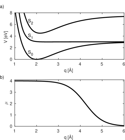
Figure 1: (a) Bare state PESs used for the photonic catalyst model as well as the photonic bound state model. The minimum of the S₂ state is displaced by 0.3 $\mathrm{\AA}$ with respect to the ground state. (b) Transition dipole curve used in the different models. The parameters for the model are given in Appendix A.

In the following we present calculations on three simple model systems to illustrate the basic possibilities of the cavity coupling and the effects on the non-adiabatic couplings. The level structure of the dressed states creates new pathways for the nuclear dynamics and new transitions for spectroscopic measurements. Our goal is to use the influence of the cavity to modify the reactivity of a molecule. Photodissociation in the dressed state basis can then be enhanced or suppressed.

III.1 Photonic Catalyst

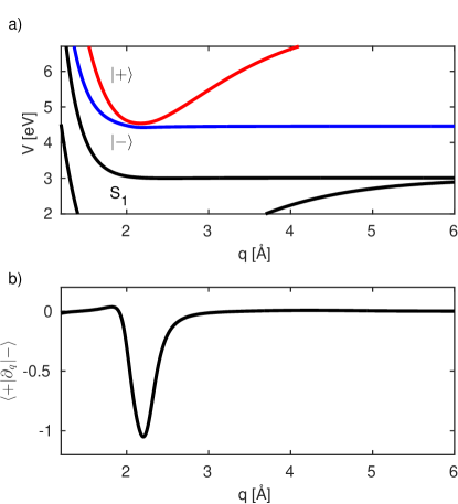
Figure 2: (a) Dressed state PESs for the photonic catalyst model. The $S_{2}$ state is now coupled to the dissociative state. (b) Non-adiabatic coupling matrix element for the polariton states. Dominated by the gradient difference term of eq. 20. Parameters: $g=54$ meV

In the first model (Fig. 1(a)) we assume that a bound state S₂ is accessible by a dipole transition from the ground state S₀. The dissociative state S₁ does not have a transition dipole moment with the ground state, but is accessible from S₂. The cavity couples the states S₂ and S₁ through the transition dipole moment shown in Fig. 1(b). The cavity mode frequency $\omega_{c}$ is set be in resonance at the minimum of S₂ (1.45 eV) and with a maximum cavity coupling of $g=54$ meV. The states $|g\rangle\equiv\mathrm{S}_{1}$ and $|e\rangle\equiv\mathrm{S}_{2}$ are used along with Eq. 13 to form the dressed states, shown in Fig. 2(a). The resulting dressed states $|\mathrm{S}_{1}\rangle$, $|-\rangle$, and $|+\rangle$ undergo an avoided crossing close to resonance, while their shape remains similar to the bare states. The corresponding non-adiabatic coupling matrix element $f_{+,-}$ (Eq. 18), which is responsible for the transition between the dressed states is shown in Fig. 2(b). The initially dark state S₁ now becomes radiatively accessible from S₀ through the non-adiabatic couplings via the S₂ state. It is evident that the dressed states are coupled to each other in the region where the bare states are close to resonance with the cavity mode. The upper dressed state – whose shape still resembles the shape of the S₂ state – is thus not stable anymore and the molecule can dissociate through the non-adiabatic coupling to the unbound lower dressed state.

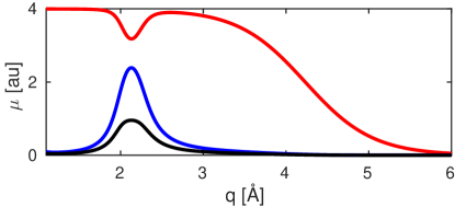
Figure 3: Transition dipole moments in the dressed state basis for the photonic catalyst model: $\mu_{g+}$ (red), $\mu_{g-}$ (blue),$\mu_{-+}$ (black).

Figure 3 displays the relevant transformed transition dipole moments calculated from Eqs. 31 to 33. All curves show a dip around 2.2 $\mathrm{\AA}$ where the non-adiabatic coupling and thus the mixing between the molecular states and the photon states is strongest. The transition dipole between the dressed states vanishes if the cavity coupling vanishes. The coupling to the cavity creates a new transition and modified dynamics which can be probed with time resolved spectroscopy.

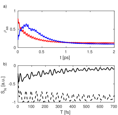
Figure 4: (a) Populations of the dressed states $|+\rangle$ (red) and $|-\rangle$ (blue) in the photonic catalyst model vs. time. The decay of the $|+\rangle$ state can be fitted to a bi-exponential model yielding the time constants 228 fs and 42 ps. (b) Transient absorption signal in depenence of the probe delay $T$ and. The laser is set to be resonant between S₁ and the $|\pm\rangle$ state (1.5 eV) and has a pulse length of 10 fs (FWHM). The dashed line is the signal for a wave packet in the S₂ bare state potential.

The excited state evolution was simulated by wave packet dynamics on a spatial grid (for details see Appendix B). Figure 4(a) depicts the dynamics after impulsive excitation from the ground state (S₀) to the dressed states $|\pm\rangle$. The initial population pattern is caused by the mixing of the transition dipole moments, followed by a rapid decay of the upper dressed state caused by the dissociative/unbound character of the lower dressed state. The oscillation pattern is caused by the wave packet oscillation in the $|+\rangle$ state, passing through the coupling region. Figure 4(b) shows the transient absorption signal (see Appendix C) probing the system via the $|g\rangle$ state. The signal shows a clear decay of stimulated emission modulated by the wave packet motion in the $|+\rangle$ state.

III.2 Photonic Bound States

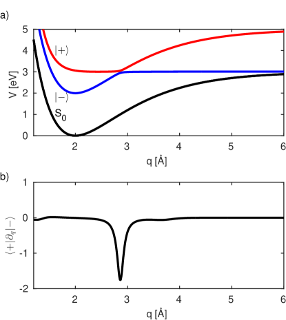
Figure 5: (a) Dressed state PESs for the photonic bound state model. (b) Non-adiabatic coupling matrix element causing transition between the dressed states.

In the second model, we reverse the roles of bound and unbound states to create a situation where a purely dissociative state can be stabilized (i.e. increase its lifetime) via cavity coupling to a bound state. We use the model from Fig. 1, but only considering states S₀ and S₁. An excitation from S₀ to S₁ causes immediate dissociation of the molecule in the bare state model. Setting the cavity mode on resonance with S₀ and S₁ at $\approx 2$ eV creates a set of dressed states, which experience an avoided crossing (Fig. 5(a)) with a non-adiabatic coupling matrix element (Fig. 5(b)) peaking at the crossing at 2.9 $\mathrm{\AA}$. The lower dressed state resembles the ground state around the Franck-Condon point and forms a bound state potential. The upper dressed state now also appears as a partially bound state potential, which is coupled to the dissociative curve by the avoided crossing.

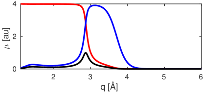
Figure 6: Tranistion dipole moments in the dressed state basis: $\mu_{g+}$ (red), $\mu_{g-}$ (blue), $\mu_{-+}$ (black).

The transition dipole moments are shown in Fig. 6. Due to the large detuning $\delta_{c}$ in the Franck-Condon region, the lower dressed state has a weak transition dipole moment with respect to the S₀ state. The state character change at the crossing at 2.9 $\mathrm{\AA}$ manifests itself in the rapid change of the transition dipole moments (the crossing of the red and blue curve in Fig. 6.).

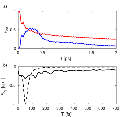
Figure 7: (a) Population of the dressed states $|+\rangle$ (red) and $|-\rangle$ (blue) in the photonic catalyst model vs. time. The decay of the $|+\rangle$ state can be fitted to a bi-exponential model yielding the time constants 234 fs and 5.2 ps. (b) Transient absorption signal. Laser is set to be resonant between S₁ and the $|\pm\rangle$ state (1.5 eV) and has a pulse length of 10 fs (FWHM). The dashed line is the signal for a wave packet in the S₁ bare state potential

The population dynamics after excitation is shown in Fig. 7(a)). The clear distribution of the dipole moments between ground state and the dressed states leads to the upper dressed state population upon impulsive excitation. The quasi-bound character of the upper dressed state becomes clear from Fig. 7(a)): Instead of immediate dissociation the upper dressed state acquires a significant lifetime. The population of $|+\rangle$ leaks into $|-\rangle$ on a picosecond time scale. The corresponding transient absorption signal is shown in Fig. 7(b)) along with the signal for the bare state system (dashed curve).

III.3 Photoninduced Conical Intersections

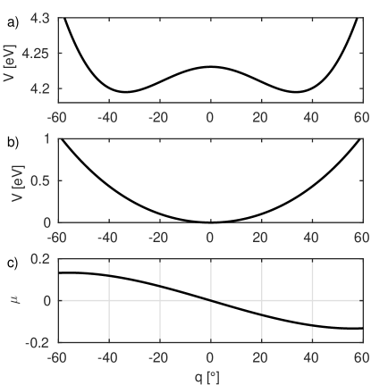
Figure 8: Bare state PESs for the photoninduced CoIn model calculated at the CAS(4/4)/MRCI/6-311G* level of theory with the program package MOLPRO Werner et al. (2010): (a) The double minimum of the $S_{1}$ state. (b) The ground $S_{0}$ ground state of formaldehyde. $q$ is the angle of the out-of-plane motion. The cavity is set in resonance at $q=0$. (c) Transition dipole moment $S_{0}\rightarrow S_{1}$.

So far we have demonstrated the non-adiabatic couplings induced by the cavity in terms avoided curve crossings, which stem from the fact that a non-vanishing dipole in the coupling region creates a splitting between the dressed states (see Eq. 9). However, by choosing a point of vanishing transition dipole moments one can in principle also create a crossing, which exhibits a degeneracy between the dressed states. This is the basic requirement to obtain a CoIn, i.e. the coupling between the adiabatic electronic states has to vanish at the intersection point Domcke et al. (2011). In our third example of light-induced CoIns Demekhin and Cederbaum (2013); Kim et al. (2015b) this condition is fulfilled by rotating the molecule with respect to the polarization vector of the driving field. By inspecting Eq. 13 we identify another type of light induced CoIn: Setting the cavity on resonance at a nuclear configuration where the transition dipole moments vanishes yields a degenerate point in the dressed state basis. This can be achieved by choosing an electronic transition which is dipole forbidden at a certain configuration of high symmetry and becomes allowed as the symmetry is lowered. We now demonstrate this case for formaldehyde. In its planar equilibrium structure the lowest energy transition from the ${}^{1}A_{1}$ state to the ${}^{1}A_{2}$ state transition is dipole forbidden. Every vibrational mode which is not of the $A_{1}$ irreducible representation breaks the $C_{2v}$ symmetry ($B_{1}$, $B_{2}$) and can be expected to make the transition dipole allowed. In Fig. 8 the potentials and transition dipole moments are shown vs. the out-of-plane motion ($B_{1}$) of the hydrogen atoms. Setting the cavity in resonance with the forbidden transition thus creates a vacuum field, light induced CoIn, which we call photoninduced CoIn.

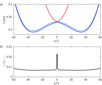
Figure 9: (a) Dressed state PESs (red: $|+\rangle$, blue $|-\rangle$) for the photoninduced CoIn model in dependence of the out-of-plane angle $\phi$. The dashed line indicates the $S_{1}$ bare state. (b) Non-adiabatic coupling matrix element for the polariton states. The splitting vanishes at $q=0$, hence the degeneracy. The cavity coupling is chosen to be $g_{max}=434$ meV.

The corresponding dressed states and the non-adiabatic coupling matrix element are shown in Fig. 9. The degenerate point appears at the planar configuration ($q_{1}=0$) along with a peaking non-adiabatic transition matrix element $f^{(1)}_{-,+}$. Note that $f^{(1)}_{-,+}$ diverges when the detuning is exactly zero. Choosing a second vibrational mode which also breaks the symmetry will create a transition dipole moment and will result in a typical cone-shaped PES. We demonstrate this feature for the asymmetric stretch motion of the CH₂ group ($B_{2}$). The resulting PES of the dressed states is shown in Fig. 10.

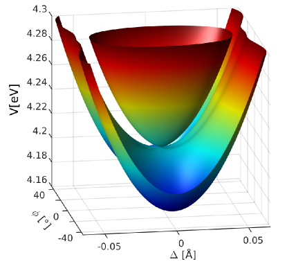
Figure 10: Photoninduced CoIn between the dressed states in formaldehyde in dependence of two vibrational modes: CH₂ out-of-plane motion ($\phi\equiv q_{1}$) and the CH₂ asymmetric stretch motion ($\Delta\equiv q_{2}$).

IV Conclusions and Outlook

We have developed a theory, which can be applied to compute the non-adiabatic dynamics of single molecules strongly coupled to a single cavity mode. The formalism expressed in terms well known derivative couplings is suitable for various simulations protocols like full quantum propagation and semi-classical methods like for example surface hopping Hammes‐Schiffer and Tully (1994) and ab initio multiple spawning Ben-Nun et al. (2000). The quantities required to express the molecular system in terms of dressed states, i.e. the potential energy surfaces and transition dipole moments can be directly obtained from state of the art quantum chemistry methods. The derivations are done within the RWA and the assumption that the ultrafast dynamics timescale is shorter than the lifetime of the photon mode. However, we could identify situations where the JC Hamiltonian is not adequately described by two photon states and higher manifolds must be taken into account for the procedure to converge. A break down of the RWA can be caused by various factors: Large detunings give rise to off-resonant terms ($a^{\dagger}\sigma^{\dagger}$ and $a\sigma$) in the ultra strong coupling regime ($g\approx\omega_{c}$) give rise to the Bloch-Siegert shift and ground state modifications. The off-resonant regime can be easily accessed by coupling close to the CoIn, while the ultra strong coupling regime might be difficult to reach due to technical limitations of the nano-structures, like for example the achievable size of the mode volume. Moreover, the applicable field strength is limited by the ionization potential of a molecule.

Some basic possibilities for the manipulation of the excited state photo chemistry have been demonstrated for photo dissociation model systems. The life time with respect to dissociation can potentially be significantly influenced by the cavity coupling. Non-adiabatic coupling between the dressed states is the cause for the coupling and the effect on the nuclear dynamics. The population transfer between the dressed states may also be viewed via stimulated emission caused by the vacuum state of the photon mode.

Single molecule strong coupling is an experimentally challenging regime and has not been demonstrates yet to the extent necessary to influence chemistry. However, coupling of a ensemble of $N$ molecules to the mode of a micro resonator, which is enhanced by a factor $\sqrt{N}$ Hutchison et al. (2012) shows promising results. The collective chemistry in a cavity is a many body effect, which needs further investigation. Its theoretical treatment is more challenging since all particles are coupled and the dimensionality increase with the number of particles. Finally the super radiant Dicke (1954) regime might be used to engineer the reactivity of molecules in a novel way.

Appendix A Model parameters

The model potentials shown in Fig. 1(a) are obtained from Morse potentials:

$$V_{i}(q)=D_{i}\left[1-\exp\left(-a_{i}(q-q_{0,i})\right)\right]^{2}+V_{0}$$ (34)

The respective parameters are given in tab. 1.

Table 1: Parameters for the potentials shown in Fig. 1.

$i$	$D_{i}$ [eV]	$a_{i}$ [Å-1]	$q_{0,i}$ [Å]	$V_{0}$ [eV]
S0	3.0	1	2.0	0
S1	0.01	2.43	2.5	3
S2	3.0	1	2.3	4.5

The transition dipole shown in Fig. 1(b) is defined by the sigmoid function:

$$\mu(q)=\dfrac{4}{1+\exp[2.4575(q-4.232)]}$$ (35)

Appendix B Quantum Propagation

The wave packet propagations are carried out on a numerical grid using the Hamiltonian from Eq. 30 where the kinetic energy is given by

$$\hat{T}=-\dfrac{1}{2m}\dfrac{d^{2}}{dq^{2}}$$ (36)

with $m=3650$ being the reduced mass. For all dissociative potentials the kinetic energy term $\hat{T}$ is replaced by a perfectly matched layer Nissen et al. (2010) to avoid spurious reflections at the edge of the grid. The time evolution is calculated with an Arnoldi propagation scheme Tannor (2006); Smyth et al. (1998).

Appendix C Transient Absorption Spectrum

The transient absorption signal is linear in the probe intensity and given as the frequency integrated rate of change in the photon number (for further details see Ref. Dorfman et al. (2015)):

$$S_{N}(T)= -\dfrac{2}{\hbar}{\cal I}\int_{-\infty}^{\infty}dt\int_{-\infty}^{t}d\tau{\cal E}^{*}(t-T){\cal E}(\tau-T)$$

$$\times\langle\Psi_{0}|U^{\dagger}(t,0)\hat{\mu}U(t,\tau)\hat{\mu}^{\dagger}U(\tau,0)|\Psi_{0}\rangle$$ (37)

where $\Psi_{0}=(\hat{\mu}_{g+}+\hat{\mu}_{g-})\Psi_{S_{0},v=0}$ is the initial wave function prepared by impulsive excitation from the vibrational ground state of the S₀ potential and $U(t,t^{\prime})=\exp\left(-i\hat{H}(t-t^{\prime})\right)$ propagates the system from $t^{\prime}$ to $t$. The propagator $U$ is implement by a numerical propagation as described in the previous section. The operator $\hat{\mu}\equiv\mu_{ij}(q)$ includes transition dipole moments between the relevant electronic stats and depends on the nuclear coordinates. The probe field is given by

$${\cal E}(t)=e^{-i\omega_{L}t-t^{2}/2\sigma^{2}}\,,$$ (38)

where $\omega_{L}$ is the center frequency and $\sigma$ the temporal width of the laser pulse and $T$ is the delay with respect to the initial state preparation.

References

- Domcke et al. (2011) W. Domcke, D. R. Yarkony, and H. Köppel, Conical Intersections, Vol. 17 (WORLD SCIENTIFIC, 2011).
- Gollub et al. (2010) C. Gollub, M. Kowalewski, S. Thallmair, and R. Vivie-Riedle, Phys. Chem. Chem. Phys. 12, 15780 (2010).
- Sussman et al. (2006) B. J. Sussman, D. Townsend, M. Y. Ivanov, and A. Stolow, Science 314, 278 (2006).
- Kim et al. (2012) J. Kim, H. Tao, J. L. White, V. S. Petrović, T. J. Martinez, and P. H. Bucksbaum, J. Phys. Chem. A 116, 2758 (2012).
- Hutchison et al. (2012) J. A. Hutchison, T. Schwartz, C. Genet, E. Devaux, and T. W. Ebbesen, Angew. Chem. Int. Ed. 51, 1592 (2012).
- Purcell (1946) E. M. Purcell, Phys. Rev. 69, 681+ (1946).
- Morigi et al. (2007) G. Morigi, P. W. H. Pinkse, M. Kowalewski, and R. de Vivie-Riedle, Phys. Rev. Lett. 99, 073001 (2007).
- Kowalewski et al. (2011) M. Kowalewski, G. Morigi, P. W. H. Pinkse, and R. de Vivie Riedle, Phys. Rev. A 84, 033408 (2011).
- Haroche and Raimond (2006) S. Haroche and J.-M. Raimond, Exploring the Quantum: Atoms, Cavities, and Photons (Oxford Graduate Texts), 1st ed. (Oxford University Press, 2006).
- Hopfield (1958) J. J. Hopfield, Phys. Rev. 112, 1555 (1958).
- Tomljenovic-Hanic et al. (2006) S. Tomljenovic-Hanic, M. J. Steel, C. M. de Sterke, and J. Salzman, Opt. Express 14, 3556+ (2006).
- Kim et al. (2015a) M.-K. Kim, H. Sim, S. J. Yoon, S.-H. Gong, C. W. Ahn, Y.-H. Cho, and Y.-H. Lee, Nano Lett. 15, 4102 (2015a).
- Faez et al. (2014) S. Faez, P. Türschmann, H. R. Haakh, S. Götzinger, and V. Sandoghdar, Phys. Rev. Lett. 113 (2014), 10.1103/physrevlett.113.213601.
- Galego et al. (2015) J. Galego, F. J. Garcia-Vidal, and J. Feist, Phys. Rev. X 5, 041022+ (2015).
- Jaynes and Cummings (1963) E. T. Jaynes and F. W. Cummings, Proc. IEEE 51, 89 (1963).
- Hood et al. (1998) C. J. Hood, M. S. Chapman, T. W. Lynn, and H. J. Kimble, Phys. Rev. Lett. 80, 4157 (1998).
- Kim et al. (2015b) J. Kim, H. Tao, T. J. Martinez, and P. Bucksbaum, J. Phys. B: At. Mol. Opt. Phys. 48, 164003+ (2015b).
- von den Hoff et al. (2011) P. von den Hoff, M. Kowalewski, and R. de Vivie-Riedle, Faraday Discuss. 153, 159 (2011).
- Pritchard et al. (2013) J. D. Pritchard, K. J. Weatherill, and C. S. Adams, Annual Review of Cold Atoms and Molecules, Annu. Rev. Cold At. Mol., Volume 1, 301 (2013).
- Hofmann and de Vivie-Riedle (2001) A. Hofmann and R. de Vivie-Riedle, Chem. Phys. Lett. 346, 299 (2001).
- Martínez et al. (1997) T. J. Martínez, M. Ben-Nun, and R. D. Levine, J. Phys. Chem. A 101, 6389 (1997).
- Werner et al. (2010) H.-J. Werner, P. J. Knowles, G. Knizia, F. R. Manby, M. Schütz, et al., “Molpro, version 2010.1, a package of ab initio programs,” (2010), see http://www.molpro.net (visited on 11/01/2015).
- Demekhin and Cederbaum (2013) P. V. Demekhin and L. S. Cederbaum, J. Chem. Phys. 139, 154314 (2013).
- Hammes‐Schiffer and Tully (1994) S. Hammes‐Schiffer and J. C. Tully, J. Chem. Phys. 101, 4657 (1994).
- Ben-Nun et al. (2000) M. Ben-Nun, J. Quenneville, and T. J. Martínez, J. Phys. Chem. A 104, 5161 (2000).
- Dicke (1954) R. H. Dicke, Phys. Rev. 93, 99 (1954).
- Nissen et al. (2010) A. Nissen, H. O. Karlsson, and G. Kreiss, J. Chem. Phys. 133, 054306 (2010).
- Tannor (2006) D. J. Tannor, Introduction to Quantum Mechanics: A Time-Dependent Perspective (University Science Books, 2006).
- Smyth et al. (1998) E. S. Smyth, J. S. Parker, and K. T. Taylor, Comput. Phys. Commun. 114, 1 (1998).
- Dorfman et al. (2015) K. E. Dorfman, K. Bennett, and S. Mukamel, Phys. Rev. A 92 (2015), 10.1103/physreva.92.023826.