Attractor non-equilibrium stationary states in perturbed long-range interacting systems

Abstract

Isolated long-range interacting particle systems appear generically to relax to non-equilibrium states (“quasi-stationary states” or QSS) which are stationary in the thermodynamic limit. A fundamental open question concerns the “robustness” of these states when the system is not isolated. In this paper we explore, using both analytical and numerical approaches to a paradigmatic one dimensional model, the effect of a simple class of perturbations. We call them “internal local perturbations” in that the particle energies are perturbed at collisions in a way which depends only on the local properties. Our central finding is that the effect of the perturbations is to drive all the very different QSS we consider towards a unique QSS. The latter is thus independent of the initial conditions of the system, but determined instead by both the long-range forces and the details of the perturbations applied. Thus in the presence of such a perturbation the long-range system evolves to a unique non-equilibrium stationary state, completely different to its state in absence of the perturbation, and it remains in this state when the perturbation is removed. We argue that this result may be generic for long-range interacting systems subject to perturbations which are dependent on the local properties (e.g. spatial density or velocity distribution) of the system itself.

I Introduction

Systems of large numbers of interacting particles are subject in their physical analysis to a fundamental distinction based on whether they are short-range or long-range, depending on the rapidity of the decay with separation of the two body interaction potential. The distinction in its canonical form arises from the presence or absence of the property of additivity of the macroscopic energy, which plays a fundamental role in equilibrium statistical mechanics. While most of familiar laboratory systems studied in physics are short-range — notably any system constituted of neutral atoms or molecules — there are numerous examples also of long-range systems, ranging from self-gravitating systems in astrophysics and cosmology, to vortices in turbulent fluids, laser cooled atoms, and even biological systems (for a review, see e.g.Campa et al. (2009, 2014)). Study of various isolated long-range systems has shown that they evolve from generic initial conditions to microscopical non-Boltzmann equilibria, known as “quasi-stationary states” (QSS) because they evolve towards the system’s true statistical equilibrium on time-scales which diverge with the number of particles (see e.g. Yamaguchi et al. (2004); Joyce and Worrakitpoonpon (2010); Levin et al. (2008); Marcos (2013); Gabrielli et al. (2010); Rocha Filho et al. (2014)) The evolution to such states appears not to be characteristic of all long-range interactions, but only of the sub-class of these interactions for which the pair force (rather than pair potential) is non-integrable at large distances (see Gabrielli et al. (2010, 2014)). As these systems remain in the QSS indefinitely in the thermodynamic limit, these states can be considered to be the fundamental relevant macroscopic equilibria of such systems, just as Maxwell Boltzmann (MB) equilibria are for short-range systems. Theoretically they are understood to be stationary solutions of the Vlasov equation which in principle describes these systems in the relevant thermodynamic limit. Unlike MB equilibria, they are infinitely numerous at given values of the global conserved quantities, and the actual equilibrium reached depends strongly on the initial condition of the system.

A basic question which arises about QSS in long-range interacting systems concerns the “robustness” of such states. They are strictly defined only for isolated Hamiltonian systems and the question is whether they continue to exist when the system is not exactly isolated, or exactly Hamiltonian, or both. For attempts to observe these intriguing equilibria in laboratory systems, which are necessarily perturbed by and coupled to the external world in some way, it is an essential to know whether these states can be expected to survive. Studies of toy models coupled to a thermal bath (see e.g. Chavanis et al. (2011)) show, unsurprisingly, that such a coupling sends the system to its thermal equilibrium, on a time scale which depends on the coupling. However, much more generally, it has been suggested on the basis of study of the one dimensional HMF model (see e.g.Gupta and Mukamel (2010a, b)) that QSS will disappear in the presence of any generic stochastic perturbation to the dynamics. A study of the effect of external stochastic fields with spatial correlation applied to the same model (see e.g. Nardini et al. (2012a, b).) shows however that interesting non-equilibrium steady states can be obtained in this case.

In this article we explore the question of the robustness of QSS in long-range systems to weak perturbations using a paradigmatic toy model of long-range interactions — a one dimensional self-gravitating system — subjected to a particular class of perturbations, which we refer to as “local internal perturbations”: the perturbations to the purely self-gravitating dynamics occur when particles collide, and are described by simple collision rules for the colliding particles, which may be stochastic or deterministic. The perturbations can thus be considered to model physical effects which come into play at very small scales e.g. due to very short scale forces and/or internal degrees of freedom. Differently to the study of Nardini et al. (2012a, b) there are therefore no external forces, and indeed we will build our collision rules so that they conserve total momentum. The choice of the two specific two models we study is then guided by simplicity: once momentum conservation is imposed, a non-trivial collision rule in one dimension cannot conserve energy (as an elastic collision gives rise simply to exchange of particle velocities). As we wish to focus here on the effect on the effect of the perturbations on QSS, which have fixed energy, we choose to define perturbations which can conserve average energy and lead (in principle) to a steady state. The two models we study are then simple choices with this property, corresponding to collision rules drawn from the literature on granular gases arising from simple considerations of energy balance. In the one dimensional self-gravitating model these perturbations given by non-trivial collision rules are both very simple to implement numerically, and, as we will see, also admit a straightforward theoretical description for the kinetic theory in an appropriate mean-field limit.

Our main result is that in both models we study we observe an evolution from the initial QSS, which arises from a given initial condition, through a family of states, until a truly stationary state is reached. The evolution is through a continuum of QSS and the final state is also a QSS: if the perturbation is removed the system remains in this state. Further the final stationary state in each case appears to be an attractor for the perturbed long-range system, i.e., starting from different initial conditions which evolve to very different QSS the perturbation drives them all finally to the same non-equilibrium state. This “universal” QSS is thus determined essentially by the detailed nature of the small perturbation and the long-range force itself.

The paper is organized as follows. We first define the two models we study of self-gravitating particles perturbed in a specific manner when particles collide. In the following section we describe analytical approaches to these models which are valid in an appropriate mean-field limit. These give rise to kinetic equations which allow us to determine a well defined large $N$ limit. They also provide predictions for the early time evolution of the system. In the next section we present results of numerical studies of the two models. In our conclusions we compare our results with other relevant works in the literature, and comment on the possible generality of the behaviours we observe in a broad class of perturbed long-range systems.

II Models

II.1 The sheet model

We consider a system of identical particles of mass $m$ moving in a one dimensional space and interacting by a force independent of their separation, i.e. the force on a particle $i$ due to a particle $j$ is

$$F_{ij}=−gm^{2}sgn(x_{i}-x_{j}),$$ (1)

where $g$ is the interaction strength. The model is known as the “sheet model” because these particles in one dimension are equivalent to infinite, infinitely thin, parallel sheets moving in three dimensions interacting by Newtonian gravity, in which case $gm=2\pi\Sigma G$, where $G$ is Newton’s constant and $\Sigma$ is the mass per unit surface area of the sheets. This model dates back at least to the early study of CammCamm (1950) and has been studied quite extensively by numerous authors since (see e.g. Miller (1996); Yawn and Miller (1997); Joyce and Worrakitpoonpon (2011) and references therein).

For a finite system of $N$ particles, the total force acting on the $i$th particle at any time is simply given as

$$F_{i}=gm^{2}[N_{i}^{+}-N_{i}^{-}],$$ (2)

where $N_{i}^{+}$ and $N_{i}^{-}$ denote the numbers of particles on the right and on the left of $i$th particle, respectively.

The dynamics of this system has been extensively studied (see e.g. Miller (1996); Yawn and Miller (1997); Joyce and Worrakitpoonpon (2011)) and shows that the time evolution of the system displays long-lived QSS before reaching equilibrium. More precisely the relaxation time associated with QSS is diverging with the system size $\tau\sim AN$, where the coefficient $A$ depends strongly on the initial states Joyce and Worrakitpoonpon (2011).

We consider now two variants of this model, in which the particle collision still conserves the momentum but not the total energy. On the other hand, as we wish the system to be able to attain a stationary state at constant energy, we constrain the exact collision rules to allow this. Both collision laws are taken from simple models of granular systems which have been studied in the literature (see references below).

II.2 Model A: collisions with random coefficients of restitution

Let us denote $v_{ij}=v_{i}-v_{j}$ the relative velocity of particles $i$ and $j$ which undergo a collision with precollisional velocities $v_{i}$ and $v_{j}$. We adopt the rule that the postcollisional velocities, $v^{*}_{i}$ and $v^{*}_{j}$, are given by

$$v_{i}^{*}= v_{j}+\frac{1-c}{2}v_{ij}$$ (3)

$$v_{j}^{*}= v_{i}-\frac{1-c}{2}v_{ij},$$

where the coefficient of restitution $c$ is a non-negative random variable. Equivalently it corresponds to momentum conservation combined with the rule

$$v_{ij}^{*}=-cv_{ij}\,.$$ (4)

Granular models of this kind, incorporating a random coefficient of restitution, have been introduced by  Barrat et al. (2001) in order to include the effect of energy injection in a vibrated two-dimensional granular gas.

In each collision the change of the kinetic energy is given by

$$\delta K=\frac{m}{4}[(v_{ij}^{*})^{2}-(v_{ij})^{2}]=\frac{c^{2}-1}{4}(v_{ij})^{2}$$ (5)

i.e. the collision is inelastic if $0\leq c<1$ and super-elastic if $c>1$. In order that the applied perturbation may admit stationary states, we choose $c$ from a bimodal probability distribution in which $c$ takes two values, $c_{A}$ and $\tilde{c}_{A}$, with equal weight, with $0<c_{A}<1$ and

$$\tilde{c}_{A}=\sqrt{2-c_{A}^{2}}$$ (6)

The latter relation imposes that, for a collision at the same initial relative velocity, the energy lost with $c=c_{A}$ is the same as the energy gained when $c=\tilde{c}_{A}$. Thus, in the ensemble of realizations of the stochastic perturbations, the average energy is constant, with the energy loss of the inelastic collisions ($0<c_{A}<1$) balanced by the energy gain in superelastic collisions ($\tilde{c}_{A}>1$). We expect that in this case the system may be able to reach a stationary state with constant energy (modulo finite $N$ fluctuations).

II.3 Model B: inelastic collisions with energy injection

In this model the self-gravitating particles undergo collisions specified by the following rule:

$$v_{i}^{*}= v_{j}+\frac{1-c_{B}}{2}v_{ij}-\epsilon_{ij}\Delta$$ (7)

$$v_{j}^{*}= v_{i}-\frac{1-c_{B}}{2}v_{ij}+\epsilon_{ij}\Delta$$

where the constant $c_{B}$ has a fixed value in the range $0<c_{B}<1$ (i.e. as for an inelastic collision), $\Delta$ is a positive constant (with dimensions of velocity) and $\epsilon_{ij}=sgn(v_{ij})$. The collision manifestly still conserves total momentum, and corresponds to

$$v_{ij}^{*}=-sgn(v_{ij})[c_{B}|v_{ij}|+2\Delta]\,.$$ (8)

and therefore the energy change is

$$\delta K=m\left[\frac{c_{B}^{2}-1}{4}v^{2}_{ij}+c_{B}\Delta|v_{ij}|+\Delta^{2}\right]$$ (9)

The term in $\Delta$ in the collision rule thus leads to an energy injection, which can be smaller or larger than the energy loss due to the inelastic term: more precisely, the collision leads to an energy gain if $|v_{ij}|<v_{0}$, and an energy loss if $|v_{ij}|>v_{0}$, where

$$v_{0}=\frac{2\Delta}{1-c_{B}}$$ (10)

is the value of the relative velocity for which the collision is elastic.

This collision rule is the one dimensional version of that introduced in two dimensions by Brito et al. (2013) in a phenomenological model of quasi-two dimensional experiments of agitated granular particles: the particles are confined between two horizontal plates, and the vibrating bottom plate transfers the kinetic energy to the particles by collisions Olafsen and Urbach (2005); Rivas et al. (2011); Néel et al. (2014). In this quasi-two dimensional geometry, the period of the vertical vibrations is much shorter than the typical time scale of the horizontal dynamics. The collision rule, Eq. (7), then represents a time coarse-grained description of the energy transfer of particle-bottom plate collisions to horizontal particle-particle collisions.

In this paper we have chosen this collision rule simply because it provides a simple way, quite different to that in the first model, to obtain a non-trivial two body collision rule which can be expected to lead to a stationary state. More specifically if the particle velocities at collisions are assumed to be uncorrelated, the kinetic energy of the system gives a direct measure of the typical relative velocity of colliding particles: $\langle(v_{i}-v_{j})^{2}\rangle=2\langle v_{i}^{2}\rangle$. The kinetic energy would then be expected to be driven towards a value of order $Nv_{0}^{2}$, as above this energy scale energy will be dissipated while below it energy will be injected. Indeed in the case in which gravity is turned off, and the particles are enclosed in a box with reflecting walls, if all particles have velocity $\pm v_{0}/2$ all collisions are elastic and the velocity distribution does not evolve at all.

Model B is in fact microscopically deterministic, while Model A is explicitly stochastic. One other notable difference is that the phase space volume occupied by particles involved in a collision strictly contracts in Model B, while it can contract or increase in Model A depending on whether the collision is inelastic or elastic. Indeed for a collision with coefficient of restitution $c$ in either model we have $dv^{*}_{i}dv^{*}_{j}=cdv_{i}dv_{j}$ which is always a contraction in Model B. This property leads to distinctive features of the long time behaviour of the models which we observe below.

III Kinetic Theory

III.1 Mean field limit without collisions

For the purely self-gravitating model the dynamics in the appropriate large $N$ mean field limit is described by the Vlasov equation Chavanis (2010); Bouchet et al. (2010); Gabrielli et al. (2014). This limit is obtained by taking $N\rightarrow\infty$ at fixed values of the total system mass $M$ and energy $E$. Denoting the mass density in phase space, $f(x,v,t)$, the Vlasov equation reads

$$\partial_{t}f(x,v,t)+J_{V}[f]=0$$ (11)

where $J_{V}[f]$ the Vlasov operator is

$$J_{V}[f]=v\partial_{x}f(x,v,t)+\bar{a}(x,t)\partial_{v}f(x,v,t)$$ (12)

where $\bar{a}(x)$ is the mean-field acceleration given by $\bar{a}(x,t)=g\int sgn(x-x^{\prime})f(x^{\prime},v^{\prime},t)dx^{\prime}dv^{\prime}$. The mass density obeys the normalization condition

$$\int\int dxdvf(x,v,t)=M\,.$$ (13)

where $M$ is the total mass of the system.

QSS are interpreted as stationary solutions of Eq.(11). There are an infinite number of such solutions, including as a particular case the statistical equilibrium of this model (see below).

III.2 Model A

III.2.1 Collision operator in Boltzmann approximation

The Vlasov equation can be derived starting from the BBGKY hierarchy and making the approximation that the two point correlations can be neglected. The collisions in our model can be treated in the same approximation, and are then described by a canonical Boltzmann operator. We thus expect our model in the mean field limit to be described by a kinetic equation

$$\partial_{t}f(x,v,t)+v.\partial_{x}f(x,v,t)$$

$$+\partial_{x}\bar{a}[f](x,t).\partial_{v}f(x,v,t)=\sum_{q}P(q)J_{q}[f,f](x,v,t)\,.$$ (14)

where, for convenience, we introduce the parameter $q=\frac{1-c}{2}$ to characterize binary collisions with a coefficient of restitution equal to $c$, and $J_{q}[f,f](x,v,t)$ is a collision operator accounting for such collisions which are assumed to occur independently with a probability $P(q)$. Initially we will leave $P(q)$ undetermined and then replace it with the specific bimodal form for Model A at the appropriate point below.

Assuming the particles to be pointlike, the collision operator is a homogeneous Boltzmann operator accounting for binary collisions, which is the sum of two contributions:

$$J_{q}[f,f](x,v,t)=G_{q}(x,v,t)-L(x,v,t)\,.$$ (15)

where $G_{q}$ is the gain term corresponding to collisions where a particle has a post-collisional velocity equal to $v$,

$$G_{q}(x,v,t) =\frac{N}{M}\int\int dv^{\prime}dv^{\prime\prime}|v^{\prime}-v^{\prime\prime}|f(x,v^{\prime},t)f(x,v^{\prime\prime},t)$$

$$\delta(v-qv^{\prime}-(1-q)v^{\prime\prime})\,,$$ (16)

and $L(x,v,t)$ is the loss term corresponding to collisions where a particle with a velocity $v$ undergoes a collision at time $t$,

$$L(x,v,t)=\frac{N}{M}f(x,v,t)\int dv^{\prime}|v^{\prime}-v|f(x,v^{\prime},t)\,.$$ (17)

Note that the loss term does not depend explicitly on the coefficient of restitution, and indeed we can write

$$J_{q}[f,f](x,v,t)=G_{q}(x,v,t)-G_{0}(x,v,t)$$ (18)

Let us introduce a series expansion of the $\delta$ function in terms of the parameter $q$

$$\delta(v-qv^{\prime}-(1-q)v^{\prime\prime})=\sum_{n\geq 0}\frac{(q(v^{\prime\prime}-v^{\prime}))^{n}}{n!}\delta^{(n)}(v-v^{\prime\prime})$$ (19)

where $\delta^{(n)}$ denotes the $n$th derivative of the $\delta$ function.

The Boltzmann operator is then expressed as

$$J_{q}[f,f](x,v,t)= \frac{N}{M}\sum_{n\geq 1}\!\int\!\!\!\int\!\!dv^{\prime}dv^{\prime\prime}|v^{\prime}-v^{\prime\prime}|\frac{q^{n}((v^{\prime\prime}-v^{\prime}))^{n}}{n!}$$

$$\delta^{(n)}(v-v^{\prime\prime})f(x,v^{\prime},t)f(x,v^{\prime\prime},t)$$ (20)

To determine whether the parameters characterizing the collisions can be rescaled with $N$ so that the collision term remains well defined (and non-trivial) in the mean-field (Vlasov) limit, we consider the limit $q\rightarrow 0$ of the model i.e. the quasi-elastic limit. Physically this is clearly the relevant limit: to obtain an $N$ independent evolution in presence of the collisions on time-scales characterizing the mean-field dynamics (e.g. the time a particle typically takes to cross the system) one must clearly “compensate” the effect of the divergent growth of the number of collisions with $N$ by making the effect of each collision arbitrarily weak.

III.2.2 Expansion of kinetic equation

Inserting Eq. (III.2.1) in the right hand side of Eq. (III.2.1) and integrating by parts term by term we obtain (following McNamara and Young (1993); Talbot et al. (2011); Joyce et al. (2014)) the collision operator given as a series of differential operators:

$$J_{A}[f] =\frac{N}{M}\sum_{n\geq 1}\left[\langle q^{n}\rangle\partial_{v}^{n}(f(x,v,t)a_{n}[f](x,v,t))\right.$$

with

$$a_{n}[f](x,v,t)=\int|v^{\prime}-v|\frac{(v^{\prime}-v)^{n}}{n!}f(x,v^{\prime},t)dv^{\prime}$$ (22)

where the brackets $\langle..\rangle$ indicate an average over the probability distribution $P(q)$. Note that $a_{1}[f](x,v,t)$ has a simple physical meaning as an average effective force due to the collisions Talbot et al. (2010); Fruleux et al. (2012).

Let us consider now the specific $P(q)$ of model A:

$$P(q)=\frac{1}{2}\delta(q-q_{A})+\frac{1}{2}\delta(q-\tilde{q}_{A})$$ (23)

where $q_{A}=\frac{1-c_{A}}{2}$ and, from the average energy conserving condition Eq.(6),

$$\tilde{q}_{A}=\frac{1-\sqrt{1+4(1-q_{A})q_{A}}}{2}$$ (24)

Expanding in ${q}_{A}$ (as $q_{A}\rightarrow 0$ in the quasi-elastic limit) we have

$$\tilde{q}_{A}=-{q}_{A}+2{q}_{A}^{2}-4{q}_{A}^{3}+O({q}_{A}^{4})$$ (25)

and thus, to leading order in powers of ${q}_{A}$ we obtain

$$\langle q^{n}\rangle= n{q}_{A}^{n+1}\quad n\,{\rm odd}$$

$$\langle q^{n}\rangle= {q}_{A}^{n}\quad\quad n\,{\rm even}\,.$$

Defining now

$${\gamma}_{A}\equiv q_{A}\,\sqrt{N}=\frac{(1-c_{A})\sqrt{N}}{2}$$ (26)

we have, at leading order in $1/N$,

$$\langle q\rangle=\langle q^{2}\rangle=\frac{\gamma_{A}^{2}}{N}$$

$$\langle q^{3}\rangle=3\langle q^{4}\rangle=\frac{3\gamma_{A}^{4}}{N^{2}}\,,$$

while, for $n>4$, $\langle q^{n}\rangle$ decreases with $N$ more rapidly than $1/N^{2}$. Thus taking the mean-field limit $N\rightarrow\infty$ at constant $\gamma_{A}$, the full expansion of the collision term reduces to the sum of the two first derivatives of $f(x,v,t)$:

$$J_{A}[f]=\frac{\gamma_{A}^{2}}{M} \left[\partial_{v}(f(x,v,t)a_{1}[f](x,v,t))\right.$$

$$\left.+\partial_{v}^{2}(f(x,v,t)a_{2}[f](x,v,t))\right]$$ (27)

Note that the non-linear structure of the integral collision operator Eq. (III.2.2) is conserved because the velocity-dependent functions $a_{n}(v)$ are functionals of $f(x,v,t)$.

We note that the crucial relation leading to the result (III.2.2) for this model is $\langle q\rangle=\langle q^{2}\rangle$, which is simply the condition of average energy conservation. Indeed from Eq. (5) it follows that the energy change in a collision at any given relative velocity is proportional to $q-q^{2}$. Thus the same mean-field limit for the kinetic theory will be obtained for any variant of this model in which $P(q)$ is such that energy is conserved on average.

We note further that in this derivation we have assumed implicitly that $f(v)$ has the convergence properties required for the validity of the Taylor expansion, which requires clearly sufficiently rapid decay of $f(v)$ at large $v$ to ensure the finiteness of the coefficients. Indeed we see that while the finiteness of Eq.(III.2.1) requires only that $f(v)$ be integrable at large $|v|$ (i.e $f(v)\sim 1/|v|^{\alpha}$ with $\alpha>2$), the definiteness of the expression Eq.(III.2.2) requires $\alpha>4$. As we will discuss below the latter assumption turns out to break down at longer times in the model.

III.2.3 Evolution of moments of velocity distribution

We now discuss some properties of the collision operator by considering the evolution of the moments of the velocity distribution. Multiplying both sides of the kinetic equation by $v^{n}$, and integrating over $v$, we obtain

$$\frac{d}{dt}[\rho(x,t)\overline{v^{n}}(x,t)]+\int dv\,v^{n}J_{V}[f]=\int dv\,v^{n}J_{A}[f]$$ (28)

where $\rho(x,t)=\int dvf(x,v,t)$ is the spatial mass density, and $\overline{v^{n}}(x,t)$ is the $n$-th moment of the velocity distribution at $x$, i.e.,

$$\overline{v^{n}}(x,t)=\int dv\,v^{n}p_{x}(v,t)\quad{\rm where}\quad p_{x}(v,t)=\frac{f(x,v,t)}{\rho(x,t)}$$ (29)

It is straightforward to show, either directly from the exact collision operator, or for each of the two terms in Eq. (28), that

$$\int dvJ_{A}[f]=0$$

$$\int dv\,vJ_{A}[f]=0$$

which express, respectively, the conservation of particle number and conservation of momentum in the collisions. Indeed it is straightforward to show that the left-hand side of Eq. (28) corresponds for $n=0$ to the continuity equation, and $n=1$ to the Euler equation.

For the case $n=2$, integration by parts using Eq. (III.2.2) gives

$$\int dv\,v^{2}J_{A}[f]=2\frac{\gamma_{A}^{2}}{M}\int dv(va_{1}[f]+a_{2}[f])f(x,v,t)$$ (30)

from which it follows using Eqs. (22) that

$$\int dv\,v^{2}J_{A}[f]=0\,,$$ (31)

which expresses the conservation of the kinetic energy by the collisions. Thus the local pressure $\rho\overline{v^{2}}$ can change only due to the mean field gravitational force (through the Vlasov flow term $J_{V}[f]$). Note that while the vanishing of the zero and first moments hold for any $P(q)$, it can be verified from Eq. (III.2.2) that the second moment vanishes only if $\langle(q-q^{2})\rangle=0$ which is, as noted above, just the condition of average energy conservation.

For any $n\geq 2$ it is straightforward to show that

$$\int dv\,v^{n}J_{A}[f]=\frac{n\gamma_{A}^{2}}{4M}\int dv\int dv^{\prime}|v-v^{\prime}|(v-v^{\prime})$$

$$\times\left[(n-3)(v^{n-1}-v^{\prime n-1})-(n-1)vv^{\prime}(v^{n-3}-v^{\prime n-3})\right]$$

$$\times f(x,v,t)f(x,v^{\prime},t)$$ (32)

from which we recover the previous result for $n=2$, and further find that the first non-zero moment is for $n=4$, and it has the simple expression

$$\int dv\,v^{4}J_{A}[f]=\frac{\gamma_{A}^{2}}{M}\int dv\int dv^{\prime}|v-v^{\prime}|^{5}f(x,v,t)f(x,v^{\prime},t)\,.$$ (33)

The fact that right hand of this expression is strictly positive has an important consequence: if this kinetic equation is valid, the system cannot reach a stationary state. Or, conversely, if the system reaches a stationary state, it must be such that the assumptions necessary for the derivation of the kinetic equation break down. As noted above we will see that our numerical study shows that the system generically evolves to such a regime. In fact, we will see that when the system reaches a stationary state it is characterized by a non-Gaussian velocity distribution with tails decaying as a power law. Indeed the estimated exponent of the velocity distribution is such that the $4$th moment is not defined and thus the above equation is not applicable in this state.

On the other hand if the system is prepared in an initial state which is a QSS, and which does satisfy the conditions necessary for the validity of the derivation leading to Eq. (III.2.2), we can use Eq. (33) to infer non-trivial information about the temporal evolution at sufficiently short times. Indeed in this case

$$\frac{d}{dt}\!\!\left(\!\rho(x,t)\overline{v^{4}}(x,t)\!\right)\!\!=\!\!\frac{\gamma_{A}^{2}}{M}\!\!\int\!\!\!dv\!\!\int\!\!\!dv^{\prime}|v-v^{\prime}|^{5}f(x,v,t)f(x,v^{\prime},t)$$ (34)

In practice we measure the integrated quantity, i.e. the rescaled fourth moment of velocity (the kurtosis), defined by

$$\beta_{2}(t)=\frac{M\int dx\int dv\,v^{4}f(x,v,t)}{\left(\int dx\int dv\,v^{2}f(x,v,t)\right)^{2}}$$ (35)

i.e. the fourth rescaled moment of the full velocity distribution $P(v,t)=\frac{1}{M}\int dxf(x,v)$. For a Gaussian distribution, the value of $\beta_{2}$ is constant, independant of the temperature of the system and equal to $3$. The time evolution $\beta_{2}(t)$ characterizes deviation of the distribution from a Gaussian distribution.

Integrating Eq. (34) over $x$ and, assuming that the time evolution of the second moment (i.e. of the total kinetic energy) can be neglected, we have

$$\frac{d\beta_{2}(t)}{dt}\simeq\frac{\gamma_{A}^{2}\int dx\int dv\int dv^{\prime}|v-v^{\prime}|^{5}f(x,v,t)f(x,v^{\prime},t)}{\left(\int dx\int dv\,v^{2}f(x,v,t)\right)^{2}}$$ (36)

We will test this prediction below for the case where the initial state is the statistical equilibrium of the system.

III.3 Model B

Following exactly the same approach we write the kinetic equation, in the Boltzmann and mean-field approximations, for this model as

$$\partial_{t}f(x,v,t)+J_{V}[f]=J_{B}[f,f](x,v,t)\,.$$ (37)

where $J_{B}[f,f](x,v,t)$ is the collision operator with the same structure as Eq. (15), but with the gain operator now given by

$$G_{q}(x,v,t) =\frac{N}{M}\int\int dv^{\prime}dv^{\prime\prime}|v^{\prime}-v^{\prime\prime}|f(x,v^{\prime},t)f(x,v^{\prime\prime},t)$$

$$\delta(v-qv^{\prime}-(1-q)v^{\prime\prime}-sgn(v^{\prime}-v^{\prime\prime})\Delta)\,$$ (38)

where $q=\frac{1-c_{B}}{2}$ is a fixed positive parameter less than unity.

Following the same arguments as above, it is clear that to obtain a collision operator $J_{B}[f,f](x,v,t)$ which is independent of $N$ in the mean-field limit, we must consider a quasi-elastic limit, with $q\rightarrow 0$ and $\Delta\rightarrow 0$ as $N\rightarrow\infty$. Further if the evolution to a stationary state is to be described in such a limit, the energy of this state, which we have inferred must be $\sim Mv_{0}^{2}$, must be extensive (like the energy in the mean field limit) and therefore $v_{0}$ must be taken independent of $N$. Now, since $\Delta=qv_{0}$, holding $v_{0}$ fixed and taking $q\rightarrow 0$ indeed defines a quasi-elastic limit.

Proceeding as in the previous case, we perform again an expansion of the Boltzmann operator in powers of $q$ about $q=0$. This gives

$$J_{B}[f,f]=\frac{N}{M}\sum_{n\geq 1}q^{n}\partial_{v}^{n}(a_{n}(x,v,t)f(x,v,t))$$ (39)

where

$$a_{n}[f](x,v,t)\!\!=\!\!\frac{1}{n!}\!\!\int\!\!|v^{\prime}-v|(v^{\prime}-v-sgn(v^{\prime}-v)v_{0})^{n}f(x,v^{\prime},t)dv^{\prime}$$ (40)

Defining now

$${\gamma}_{B}\equiv q{N}=\frac{(1-c_{B})N}{2}$$ (41)

and taking $N\rightarrow\infty$ at constant $\gamma_{B}$, we obtain a finite limit for the collision operator which corresponds to the mean field limit. In this case only the leading linear term of the expansion contributes, and the effect of collisions corresponds to the presence of an effective velocity dependent force per unit mass $a_{1}(x,v)$:

$$J_{B}[f] =\frac{\gamma_{B}}{M}\left[\partial_{v}(f(x,v,t)a_{1}[f](x,v,t))\right]\,.$$ (42)

We note that the diffusive term which was non-zero in the mean-field limit of Model A thus vanishes for Model B.

As for the model A, we can calculate the velocity moments of the collision operator $J_{B}[f]$. The first two moments again vanish as a consequence of conservation of particle number and momentum, while

$$\int dvv^{2}J_{B}[f]=2\frac{\gamma_{B}}{M}\int dvva_{1}[f]f(x,v,t)$$ (43)

Differently to model A this is not zero, in general: indeed the model does not necessarily conserve energy on average. On the other hand we expect the system to be able to reach a stationary state in which the collision operator is zero, and in this case Eq. (43) will vanish.

IV Numerical results

IV.1 Simulation method and units

IV.1.1 Code

The molecular dynamics of a one dimensional self-gravitating model is conveniently simulated using an event-driven algorithm as between particle collisions trajectories can be calculated explicitly. Such an algorithm is exact up to the machine rounding error in computing the solutions of quadratic equations giving the collision times (see Miller (1996); Joyce and Worrakitpoonpon (2011); Joyce and Sicard (2011) and references therein). Further the algorithm may be sped up using a “heap structure” Noullez et al. (2003) and by updating positions at each step only the particles involved in each collision. It is straightforward to modify this algorithm to implement the simple collision rules of our two models instead of elastic collisions (equivalent to particle crossings). We use a modified version of the code described in Joyce et al. (2014) (and greater detail in Joyce and Sicard (2011)) . Model A is characterized by the choice of the parameter $c_{A}<1$, and each collision is then chosen with probability $0.5$ to be inelastic (with $c=c_{A}$) or superelastic (with $c=\tilde{c}_{A}$). For model B is characterized fully by the values of $c_{A}$ and $\Delta$.

IV.1.2 Initial conditions

For both models we study evolution starting from three kinds of initial conditions:

• “Rectangular waterbag”: particles are randomly distributed with uniform probability in a rectangular region of phase space, $[-L_{0}/2,L_{0}/2]\times$ $[-V_{0}/2,V_{0}/2]$. For the case of gravity only, which has no characteristic length scale, this is a one parameter family of initial conditions which may be conveniently characterized fully by the initial virial ratio $R_{0}$ (and the particle number $N$), where the virial ratio $R$ (at any time) is defined as

  $$R=\frac{2K}{U}$$ (44)

  where $K$ is the kinetic energy and $U$ the potential energy. A virialized system this has $R=1$.

• Thermal equilibrium: the statistical equilibrium of the purely self-gravitating system in the micro-canonical and canonical ensemble has been derived for any finite $N$ by Rybicki (1971) and its mean-field limit (derived earlier by Camm (1950)) is

  $$f(x,v)=\frac{M}{2\sqrt{\pi}\sigma\Lambda}e^{\frac{-v^{2}}{\sigma^{2}}}\operatorname{sech}^{2}\left(\frac{x}{\Lambda}\right)$$ (45)

  with $\sigma^{2}=\frac{4E}{3M}$, $\Lambda=\frac{4E}{3gM^{2}}$ and $E$ is the total energy.

IV.1.3 Units

For our study the only dimensional parameters of relevance are the time, and, in model B, the velocity (because of the parameter $\Delta$). A natural choice of units for both are those characteristic of the mean field dynamics. For the time unit we choose

$$\tau_{dyn}=\frac{1}{\sqrt{g\rho_{0}}}\,,$$ (46)

where $\rho_{0}$ is the initial mass density of the system, and for the velocity

$$v_{dyn}=\sqrt{\frac{2E_{0}}{3M}}$$ (47)

where $E_{0}$ is the initial energy. With this definition $v_{dyn}^{2}$ is the velocity dispersion of a virialized system with energy $E_{0}$.

Previous studies (see e.g. Joyce and Worrakitpoonpon (2011)) of evolution from this first class of initial conditions for the self-gravitating system show that the system evolves, in a time of order $10-100$ $\tau_{dyn}$, to QSS of which the properties depend strongly on $R_{0}$. At longer times, of order $(10^{2}-10^{3})N\tau_{dyn}$, the different QSS all relax to thermal equilibrium Joyce and Worrakitpoonpon (2010).

IV.1.4 Additional macroscopic observables

To monitor in a simple way the evolution of the global properties of the system, we measure in addition to the energy and the virial ratio, that of a global parameter which is a simple measure of the “phase space entanglement” of the state of the system:

$$\phi_{11}=\frac{\langle|xv|\rangle}{\langle|x|\rangle\langle|v|\rangle}-1$$ (48)

As shown in Joyce and Worrakitpoonpon (2011) the only stationary solution of the Vlasov equation which is a separable function of position and velocity is that corresponding to thermal equilibrium. Thus if $\phi_{11}$ is constant and non-zero this indicates that the system is in a QSS distinct from thermal equilibrium, and its amplitude can be taken roughly as a measure of “proximity” to the latter. We also monitor the evolution of the kurtosis $\beta_{2}$ as defined in Eq. (35).

IV.2 Model A

As seen in section III.2, the relevant parameter characterizing the perturbations due to collisions in the mean-field limit is $\gamma_{A}$ defined in Eq. (26). If this limit describes accurately the dynamics of the system, the term arising from the perturbations is proportional to $\gamma_{A}^{2}$, and thus the time scale on which they are expected to modify the evolution of the system is $\sim\tau_{dyn}/\gamma_{A}^{2}$. In order to study the desired range of weak perturbation, and assess the validity of the mean-field limit, we will thus consider small values of $\gamma_{A}$ and vary $N$ keeping $\gamma_{A}$ fixed. We report here results for $\gamma_{A}=0.03$ and $\gamma_{A}=0.1$, and for $N$ in the range $N=128$ to $N=1024$. We average our results over a large number of realizations in each case.

IV.2.1 Evolution of energy and virial ratio

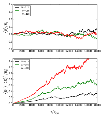
Figure 1: Model A: (Top panel) Dimensionless energy $\langle E\rangle/E_{0}$ ($E_{0}$ is the initial energy) and (bottom panel) dimensionless variance $(\langle E^{2}\rangle-\langle E\rangle^{2})/E_{0}^{2}$ versus dimensionless time $t/\tau_{dyn}$ averaged over $100$ realizations with $\gamma_{A}=0.03$, of rectangular waterbag initial conditions for $N=128,256,512$ particles.

We have constructed this model so that the fluctuations in energy of the system should become arbitrarily small for sufficiently large $N$. Indeed in the mean field limit we have derived above the energy is exactly conserved, and this limit evidently thus does not describe effects associated with the energy fluctuations at finite $N$. In our numerical study, at finite $N$, we therefore need to check whether, on the time scale simulated, the energy fluctuations are indeed small. Fig. 1 shows the evolution as a function of time of the mean energy, for a model with $\gamma_{A}=0.03$, in an ensemble of realizations starting from waterbag initial conditions with the different indicated $N$, over a time scale roughly an order of magnitude greater than $\tau_{dyn}/\gamma_{A}^{2}$. We see that, on these time scales, that in all cases, the ensemble averaged energy is indeed very close to constant, but (lower panel), the variance of the normalized energy (i) grows almost linearly in time, as indicated by the dashed straight lines and (ii) monotonically decreases as $N$ increases. Thus, as we would expect, taking $N$ sufficiently large at any given time, we can in principle converge to arbitrarily precise conservation of the energy in any single realization. In our numerical simulations at (relatively small) finite $N$, we have, however, significant finite $N$ fluctuations developing in all cases at times a few times $\tau_{dyn}/\gamma_{A}^{2}$, so we might anticipate that such effects may begin to play a significant role on these time scales.

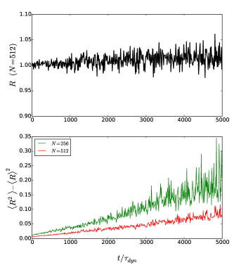
Figure 2: Model A: (top panel) virial ratio $R$ as a function of time $t/\tau_{dyn}$ averaged over $100$ realizations with equilibrium initial conditions and for $\gamma_{A}=0.03$ and $N=512$. (Bottom panel) variance of the virial ratio for $N=512$ and $N=256$ with the same initial conditions.

Fig. 2 shows the evolution of the mean (upper panel) and standard deviation (lower panel) of the virial ratio in the same ensemble of simulations as in the previous figure. Because of the equilibrium initial conditions, the system remains always, as we would expect, very close to virialized, with only finite small $N$ fluctuations which (lower panel) clearly decrease monotonically as $N$ increases. We will see below that the non-trivial time dependence of these fluctuations are a reflection of the macroscopic evolution of the system on the same time scales.

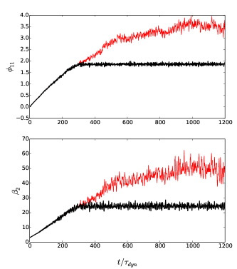
Figure 3: Model A: Evolution of the entanglement parameter $\phi_{11}$ (top panel) and of the dimensionless kurtosis $\beta_{2}$ averaged over $100$ realizations with $\gamma_{A}=0.1$ and equilibrium initial conditions for $N=1024$. The black curves correspond to a modified simulation in which the perturbation is switched off for $t\geq 300\tau_{dyn}$.

IV.2.2 Macroscopic evolution due to perturbation

Fig. 3 shows the time evolution of the entanglement parameter $\phi_{11}$ and the rescaled kurtosis $\beta_{2}$ (both defined above), averaged over $100$ realizations of equilibrium initial conditions with $N=1024$ particles. As expected, at $t=0$, $\phi_{11}=0$ and $\beta_{2}=3$: the equilibrium state phase space density is a separable function of space and velocity, and the velocity distribution has a Maxwell-Boltzmann shape. The red curve corresponds in each case to the evolution with $\gamma_{A}=0.1$, while the black curve is the evolution when this perturbation is “switched off” at the time $t=300\tau_{dyn}$, i.e., starting from this time the evolution is that of the purely self-gravitating system. Note that in line with what would be expected from mean-field theory, the characteristic time for the macroscopic evolution is about ten times shorter than in the data in the previous figures, for the case $\gamma_{A}=0.03$. We see that the evolution induced by the perturbation is through a continuum of QSS, i.e., at all times the system remains very close to a stationary and stable state of the Vlasov equation. Given that the perturbation is weak — in the sense that it perturbs the system macroscopically on a time scale long compared to $\tau_{dyn}$ — this is indeed what one would expect. However, what is not evident, and to be underlined, is that

• the effect of the small perturbation is not, at sufficiently long times, perturbative: the system is clearly progressively driven very far from its initial state. This contrasts strongly to the behaviour one would expect for familiar short range systems in which a small perturbation would be expected (e.g. applying linear response theory) to evolve to an out of equilibrium state close to the initial one, in the sense that all macroscopic quantites are changed perturbatively.

• the parameter $\phi_{11}$, which in absence of the perturbation would remain stable at its initial value $\phi_{11}=0$, evolves to a final value $\phi_{11}\approx 2-3$ depending on $N$, i.e., towards a state in which the correlation between position and velocity is ever stronger. The perturbation clearly drives the system away from thermal equilibrium.

IV.2.3 Validity of mean-field kinetic theory

Let us now consider the degree to which the evolution in our simulations of the system are described well by the mean-field limit of the kinetic equations derived above. The most basic prediction of this theory is that, when we adopt the associated scalings of the parameters with $N$, we observe an evolution which is independent of $N$. The upper two panels of Fig. 4 show respectively the evolution of $\phi_{11}$ and $\beta_{2}$, in each case averaged over $300$ realizations of the model with $\gamma_{A}=0.03$ starting from equilibrium initial conditions, and for the different particle numbers indicated: $N=128,256,512$. In both cases we observe that at sufficiently early times there is a non-trivial evolution of the system which is very well superimposed for the different $N$, indicating the validity of the mean-field theory. Further the evolution of $\beta_{2}$ at these times agrees well with that predicted by the mean-field kinetic theory at early time, shown as a straight line obtained using Eq. (36) with $f(x,v)$ taken equal to the initial thermal equilibrium phase space density Eq. (45). At longer times however we see that the evolution changes: for each $N$, the evolution breaks away, at a time scale which appears roughly to increase with $N$, from the common behaviour, and shows on a similar time scale a tendency to reach a plateau, indicating in principle the attainment of a stationary state. By measuring the velocity and spatial distributions below we will verify that this is indeed the case, and in so doing also find the explanation for the $N$-dependence and the noisiness of the evolution of $\phi_{11}$ and $\beta_{2}$ at longer times: the stationary state to which the system evolves is in fact one for which these particular macroscopic variables become ill defined in the mean field limit. This is the case because these states are characterised by velocity and spatial distributions which have slowly decaying power-law tails at long distances, for which both $\langle|x|\rangle$ and $\langle v^{4}\rangle$ diverge. Their values in a finite simulation are then regulated by the cut-off due to the finite particle number, and are thus highly fluctuating. Shown in the lower panel of Fig. 4 is the evolution of $\langle|v|\rangle$, which, in contrast, is a well defined quantity in the final state. In this case we see that the evolution for different $N$ in the mean-field scaling agrees well, and fluctuates little, right up to the time at which the stationary state is attained. The small deviation at the latest times for $N=128$ is a result of the large fluctuations of the total energy in this case (see Fig. 1 ).

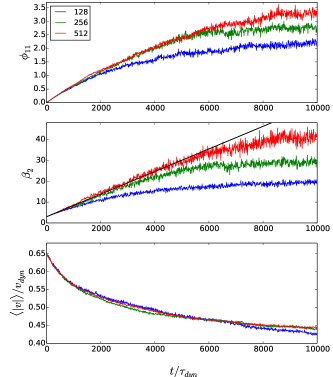
Figure 4: Model A: Entanglement parameter $\phi_{11}$, dimensionless kurtosis of the velocity distribution $\beta_{2}$ and $\langle|v|\rangle/v_{dyn}$, averaged over $300$ realizations, as functions of time $t/\tau_{dyn}$ for $\gamma_{A}=0.03$ and $N=128,256,512$ (from top to bottom).

IV.2.4 Dependence on initial conditions

Fig. 5 shows the evolution of $\phi_{11}$ and $\langle|v|\rangle/v_{dyn}$ for $\gamma_{A}=0.03$ and $N=512$ and with three different initial conditions: thermal equilibrium, and two rectangular waterbags, $R_{0}=1$ and $R_{0}=0.01$. The number of realizations are $300,100,200$ respectively. At long times, these quantities evolve towards the same mean value, independently of the initial conditions. Note that for $\phi_{11}$ fluctuations increase with time and are associated with the long tails of position and velocity distributions.

In the presence of the perturbation, the system goes at long times to a non equilibrium stationary state which is an attractor of the dynamics, i.e., the perturbed dynamics of this long-range system has a “universal” stationary state.

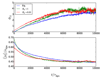
Figure 5: Model A: $\phi_{11}$ (top) and of $\langle|v|\rangle/v_{dyn}$ (bottom) as a function of time $t/\tau_{dyn}$, with $\gamma_{A}=0.03$ and $N=512$ for different initial conditions: thermal equilibrium (averaged over 300 realizations), rectangular waterbags with $R_{0}=1$ (100 realizations), and $R_{0}=0.01$ (200 realizations).

IV.2.5 “Universal” final state

Let us consider now the properties of this apparently stationary state, and check in particular whether the phase space distribution is indeed stationary and the same in the different cases.

Fig. 6 shows the velocity probability distribution averaged over $100$ realizations, for $\gamma_{A}=0.1$ and $N=1024$ and with an initial thermal distribution (black curve in the left panel). The analogous spatial distributions are shown in Fig. (7) for the same data. In both cases the relevant variable has been normalised to the square root of its variance at the given time. Except for the initial distribution (cf. Eq. 45) and the next time plotted ($t=500\tau_{dyn}$), all the curves are thereafter very well superimposed. The tail of the corresponding velocity distribution is well fitted by a simple power-law behaviour $\sim v^{-\kappa}$, with $\kappa\approx 3$, while that of the spatial distribution by $\sim x^{-\epsilon}$, with $\epsilon\approx 2$. We find the same behaviours for our different initial conditions, and for the different $N$ in the range we have considered. Further we note that we find these behaviours to be stable even if we extend our analysis to data at longer times, in which the fluctuations of energy become large. Thus the state appears to a very robust attractor even when the energy can vary considerably. As anticipated above, these asymptotic behaviours of the evolved system explain why we observed the strongly $N$ dependent behaviours of the parameters $\phi_{11}$ and $\beta_{2}$: for such asymptotic behaviours of the velocity and space distribution these quantities are divergent, and thus in practice, when measured in a system with a finite number of particles, they are dominated by the contribution from just a few of the highest energy particles.

We note that the velocity distribution observed is very similar to that found for the original purely granular model (i.e.without gravity) Barrat et al. (2001). As in this case one must in fact suppose that $\kappa>3$ to ensure that the kinetic energy (proportional to the velocity dispersion) of the state be finite.

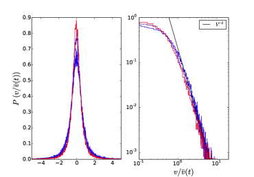
Figure 6: Model A: Velocity distribution at different times ($t=0,500,1800,2500,3700\tau_{dyn}$) averaged over $100$ realizations for $\gamma_{A}=0.1$, $N=1024$ with initial thermal distribution. Velocities are normalised by $\overline{v}(t)$, the standard deviation of the velocity distribution. The left panel is a linear plot and the right panel a log-log plot.

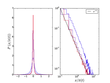
Figure 7: Model A: Position distribution at different times ($t=500,1800,2500,3700\tau_{dyn}$) averaged over $100$ realizations for $\gamma_{A}=0.1$, $N=1024$ with initial thermal distribution. Positions are normalised by $\overline{x}(t)$, the standard deviation of the position distribution. The left panel is a linear plot and the right panel a log-log plot.

IV.3 Model B

We have seen that the contribution from collisions in Model B is characterized in the mean field limit by the dimensionless parameter $\gamma_{B}$, and the velocity scale $v_{0}$, with both being held fixed in the mean-field limit. As the mean-field scaling leaves invariant also the characteristic velocity $v_{dyn}$ defined in Eq. (47), we can define the dimensionless ratio

$$u_{B}=\frac{v_{0}}{v_{dyn}}$$ (49)

which also remains fixed in the mean field limit. We then can characterize our simulations by the dimensionless parameters $\gamma_{B}$, $u_{B}$ and $N$, and the results will then be $N$-independent at sufficiently large $N$ if the mean-field treatment is valid.

IV.3.1 Macroscopic evolution due to perturbation

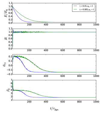
Figure 8: Model B: Dimensionless energy $E/E_{0}$ ($E_{0}$ is the initial energy), virial ratio $R$, entanglement parameter $\phi_{11}$ and dimensionless kurtosis $\beta_{2}$ versus $t/\tau_{dyn}$ for $u_{B}=1$, $\gamma_{B}=0.01,0.005$, $N=512$ and initial rectangular waterbag conditions $R_{0}=0.01$. Simulation results are averaged over $20$ realizations.

Fig. 8 shows results for the evolution of the dimensionless energy $E/E_{0}$ ($E_{0}$ is the initial value), of the virial ratio $R$, $\phi_{11}$ and $\beta_{2}$, for $N=512$, $u_{B}=1$ and rectangular waterbag initial conditions with $R_{0}=0.01$. the two curves correspond to the different values of $\gamma_{B}=0.01,0.005$ with an average over $20$ realizations. We observe that, as expected, the system reaches virial equilibrium on a time scale $\sim 10\tau_{dyn}$ and remains, to an extremely good approximation, virialized thereafter. Compared to model A, the finite $N$ fluctuations are extremely small. As we will see in further detail below, this is a result of the presence of a well defined energy scale in the model to which the system is efficiently driven. Thus the system evolves on a time scale $\sim\tau_{dyn}/\gamma_{B}$ as expected from the mean-field kinetic theory, through a continuum of QSS. Indeed, to test this conclusion, we have performed again simulations in which we “turn off” the perturbation at different times. We find, as in model A, that the macroscopic parameters remain essentially frozen at their values at this time.

For the chosen value of $u_{B}=1$ the simulations start with an energy which turns out to be about an order of magnitude larger than the energy in the stationary state. This means that the characteristic velocities are initially so large that most collisions are inelastic and the evolution depends little on the presence of the term depending on $v_{0}$. In this case the evolution is then well approximated by the case of purely inelastic collisions which we have studied in Joyce et al. (2014). For smaller values of $\gamma_{B}$ than those shown here the validity of this approximation is sufficiently extended in time so that one can see the presence of an approximate plateau in $\phi_{11}$ corresponding to the “scaling QSS” derived in this work.

IV.3.2 Dependence on initial conditions

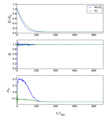
Figure 9: Model B: $E/E_{0}$ (top) and $\phi_{11}$ (bottom) versus time $t/\tau_{dyn}$ for $N=512$, $\gamma_{B}=0.01$, $u_{B}=1$ with rectangular waterbag initial conditions, $R_{0}=0.01,1$.

Fig. 9 shows the evolution of the energy $E/E_{0}$, $R$ , and $\phi_{11}$ for $\gamma_{B}=0.01$, $u_{B}=1$, $N=512$ and for two different rectangular waterbag initial conditions, $R=0.01$ and $R=1$). We see, as indicated by the behaviour of $\phi_{11}$, that each of the two initial conditions initially evolves to a quite different QSS, but then on the longer time scale both converge towards an identical value of $\phi_{11}$. That this indeed corresponds to evolution to the same final state is confirmed, as we will detail further below, by study of the final configuration in phase space.

IV.3.3 Mean-field limit of kinetic theory

To test the validity of the mean-field limit derived in Section III.2, we have run sets of simulations for the same initial conditions with fixed values of $\gamma_{B}$ and $u_{B}$, but different values of the particle number $N$. Fig. 10 shows the evolution of the energy $E/E_{0}$ (top ) and $\phi_{11}$ (bottom) for $\gamma_{B}=0.01$, $u_{B}=1$, and for rectangular waterbag initial conditions, $R_{0}=0.01$ with different system sizes, $N=128,256,512$. We see in the evolution of the energy an almost perfect superposition of the curves, indicating thus an $N$ independent evolution corresponding to the mean-field limit.

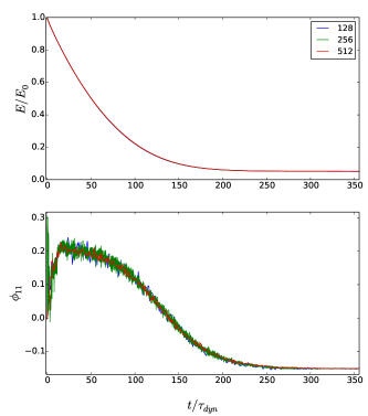
Figure 10: Model B: $E/E_{0}$ (top) and $\phi_{11}$ (bottom) for $\gamma_{B}=0.01$, $u_{B}=1$, and for rectangular waterbag initial conditions, $R_{0}=0.01$ with different system sizes, $N=128,256,512$.

IV.3.4 Properties of “universal” final state

We finally consider in greater detail the properties of the apparently very well defined final state to which the system is driven very efficiently in Model B. Fig. 11 shows snapshots, at the indicated times, of the phase space of particle positions in dimensionless units (where $x_{0}=v_{0}\tau_{dyn}$) in $20$ realizations with $N=128$ of $R=0.01$ waterbag initial conditions, for a model with $\gamma_{B}=0.01$ and $u_{B}=1$. The phases of the evolution, already evident in the evolution of the energy and $\phi_{11}$ as discussed above, are again clearly visible. However the phase space plot reveals that, from the time (here about $150\tau_{dyn}$) at which the macroscopic diagnostics indicate the establishment of the stationary states, and do not themselves appear to evolve anymore, there is a further non-trivial evolution in phase space of the microscopic particle distribution: the particles progressively “aggregate” onto distinct separated curves. A study of the particle energies shows that they are, to a very good approximation, constant on each curve, and take well separated values on each curve i.e. they are effectively discretized.

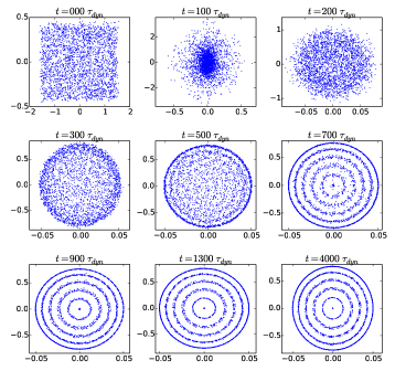
Figure 11: Model B: Phase space snapshots in dimensionless units ($x/x_{0}$ and $v/v_{0}$) for $N=128$, $\gamma_{B}=0.01$, $u_{B}=1$, rectangular waterbag initial conditions, $R_{0}=0.01$ and $20$ realizations at different times $t$ ranging from $t=0$ to $t=4000\,\tau_{dyn}$).

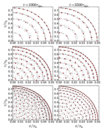
Figure 12: Model B: Phase space snapshots in dimensionless units ($x/x_{0}$ and $v/v_{0}$) for $\gamma_{B}=0.01$, $u_{B}=1$, rectangular waterbag initial conditions, $R_{0}=0.01$, $20$ realizations and at two different times $t=1000\tau_{dyn}$ (left panels), $t=3500\tau_{dyn}$ (right panels). We compare three different system sizes $N=128,256,512$ (from top to bottom). Red dots correspond to one chosen realization, small black dots correspond to the other realizations.

Fig. 12 shows phase space configurations at two times ($t=1000\tau_{dyn}$ on left, $t=3500\tau_{dyn}$ on right) for $20$ realizations of the same waterbag initial condition, and the same $\gamma_{B}$ and $u_{B}$, as in the previous figure, for $N=128$ (upper panels), $N=256$ (middle panels) and $N=512$ (bottom panels). In each plot the particle positions for a single chosen realization are also plotted as red stars. These plots show clearly that in all cases the system evolves towards a highly ordered distribution, in which the particles are not only on “shells” in phase space as noted above, but also have highly ordered positions along these shells i.e. the relative phases of the particle’ motions on the shells are fixed in time and completely coherent. Further the time scale to attain the final state appears to grow strongly with $N$ (in units of $\tau_{dyn}$): the $N=128$ simulations have already attained the completely ordered state at $t=1000\tau_{dyn}$, the $N=256$ simulations are close to attaining it for $t=3500\tau_{dyn}$, while the $N=512$ systems are still evolving towards it at this later time.

This evolution of the system towards the “ordered” state thus occurs on a time scale which diverges when we take the mean-field limit. Indeed it is an evolution intrinsically characteristic of the finite $N$ system. However, as far as we can determine, the macroscopic properties of the system are unchanged by the corresponding microscopic evolution e.g. the total energy and parameters $\phi_{11}$ and $\beta_{2}$ do not evolve on average. Thus the QSS, which corresponds to the phase space density in the infinite $N$ limit, appears to remain unaltered. This behaviour can be contrasted with the relaxation to thermal equilibrium of QSS attained in the purely self-gravitating model. This relaxation is also driven by finite $N$ effects, but it causes the system to evolve (on a time-scale $\sim N\tau_{dyn}$) through a family of QSS until it finally equilibrates.

As mentioned in Section IV.3.1 above, we have verified that the intermediate states the system evolves through from the time it virializes are indeed a family of QSS of the purely self-gravitating model: when we turn off the perturbation any time after virialization, the system’s macroscopic properties do not change on mean field time scales. For a few cases with $N=128$ we have evolved them long enough to see that, as expected, they then evolve towards thermal equilibrium on a time scale $\sim N\tau_{dyn}$. Performing the same experiment starting from a time at which the same system has had time to evolve to the “ordered” microscopic state we find an intriguing result: this ordered microscopic state remains unchanged under the purely gravitational evolution, not only on the mean-field time scale ($\tau_{dyn}$ and $\tau_{dyn}/\gamma_{B}$) but even on the time scale much greater than $N\tau_{dyn}$. Thus the microscopic state attained at long times in presence of the perturbation appears to be a periodic or quasi-periodic solution of the pure gravitational $N$-body system, and to belong to a stable island in the $N$-body phase space which leads to a breaking of ergodicity. We will investigate further both the dynamics giving rise to and the properties of these intriguing “ordered” states of the $N$-body system in future work.

V Discussion and conclusion

We have investigated the effects on the dynamics of long-range interacting systems of a class of “local internal” perturbations through the study of a canonical one dimensional toy model subjected to such perturbations. More specifically we consider two perturbations inspired by granular studies of the dynamics of a one dimensional self-gravitating system considering momentum conserving, and energy violating, collisions which are designed so that they can, nevertheless, conserve energy in an average sense. Our main focus has been on the question of how the characteristic non-equilibrium stationary states or QSS of the long-range system are affected by these perturbations. We consider the case that these perturbations are weak, in the sense that the time scale on which they affect the system macroscopically are long compared to the time scales characteristic of the dynamics of the mean gravitational field.

We have derived first kinetic equations for both models which describe the system’s evolution in a large $N$ mean-field and quasi-elastic limit. Our numerical study of the models shows that this limit describes well the macroscopic evolution due to the perturbations at sufficiently large $N$, but at given $N$ we see always also at sufficiently long times evolution in both models which are finite $N$ effects not captured by the mean field treatment. In model A such effects are manifest in large excursions of the energy at longer times, and in model B in the appearance of a highly ordered microscopic phase space distribution. Within the regime of validity of the mean field approximation both models show at longer times evolution towards an apparently unique virialized state. This state is not the thermal equilibrium of the isolated model, and indeed is typically “further away” (in terms of correlations measured by $\phi_{11}$) from the thermal equilibrium. Therefore we observed compelling evidence for the establishment of an attractor “universal” non-equilibrium stationary state in both models. Despite the stochasticity of the dynamics, explicit in model A, the system shows no tendency to relax toward equilibrium (as observed for example in the HMF model Gupta and Mukamel (2010a))

Both perturbations, which act microscopically and locally, thus completely modify the global organisation of the system: they drive the long-range system far from the QSS it is in initially (due to mean-field relaxation from the initial conditions on time scales significantly shorter on which the perturbations act). In this sense the QSS are not robust to such perturbations, and are modified macroscopically as soon as the perturbation starts to act. However, the evolution which results is through a succession of virialised states which are stationary solutions of the Vlasov equation. In both models the system is then driven finally to a non-equilibrium stationary state (NESS), which is itself also a QSS of the unperturbed long-range system. This final state does not depend on the initial conditions, but does depend strongly on the details of the perturbation. Indeed in the two models we have considered the final state has completely different properties, with notably in model A a power-law decaying space and velocity distribution compared to a phase space distribution with compact support for Model B. Thus the perturbation, albeit apparently very weak, turns out to completely dominate and determine the behaviour of the long-range system. This contrasts dramatically with the effect such a weak perturbation would have on a short range system which relaxes efficiently to thermal equilibrium: in this case the perturbation would indeed just perturb slightly this equilibrium.

It is interesting to compare our results with related previous work in the literature. In Gupta and Mukamel (2010a, b) the stochastic perturbation applied to the long-range system (the HMF model) permutes the momenta of triplets of particles chosen randomly in the system, and drives the system to relax to thermal equilibrium efficiently. Applied to a one dimensional self-gravitating system, we have checked that we observe the same behaviour. Indeed it suffices in this case to consider exchanges of the velocities of randomly chosen pairs of particles because the QSS are inhomogeneous. This drives the system efficiently to equilibrium because it destroys directly, because of the non-locality of the perturbation, the entanglement in space and velocity of the phase space distribution. In the models we have presented here the perturbation, as we have underlined, has the property of being local. This means that the instantaneous change of the velocity distribution induced by the collisions depends on the local properties, and as these typically vary in space in a non-trivial manner there is no reason to expect the system to evolve towards the same velocity distribution everywhere. On the contrary, as we have seen, the system tends to evolve towards configurations in which the space and velocity distributions are ever more strongly entangled, until a stationary state is reached in which the spatial organisation induced by the long-range forces “compensates” the local modification of the velocity distributions by the perturbations.

Our study is complementary also to that of references  Nardini et al. (2012a, b) in which the effect of an external stochastic force acting on a long-range system is studied. Indeed we can consider the perturbations we have introduced at particle collisions as stochastic forces, with the difference that they are internal, i.e. they are determined by the instantaneous microscopic state of the system itself. As we have mentioned, our models are thus appropriate to model the effects, for example, of additional short-range interactions at play in the system, while that of Casetti and Nardini (2012) models the effects of interactions with matter external to the system. For their treatment with kinetic theory, our models admit a considerable simplification compared to that required for the models of  Nardini et al. (2012a, b): as we have seen, we obtain in both our models a non-trivial kinetic theory which includes the effect of the perturbation in the mean-field limit, i.e., by neglecting two point correlations in phase space. As described in  Nardini et al. (2012a, b) a non-trivial large $N$ limit for the evolution induced by the external perturbation is obtained going beyond the mean field limit, and specifically can be obtained by including non-trivial two point correlations. The reason for this difference is that the action of the external forces on the system depend crucially on the spatial correlations of these forces, and their effect on the evolution cannot be described self-consistently without incorporating the resultant correlations in the perturbations to the phase space distributions. While Nardini et al. (2012a, b) can obtain a range of different behaviours from the external stochastic forces — ranging from thermalisation of the system to out of equilibrium states characterised by intermittency — our models display the simpler phenomenology of attractive non-equilibrium steady states we have described.

We have constructed our models so that they either conserve energy on average (model A, in the large $N$ limit) or can attain states in which energy is stationary (model B). When considering perturbations to such systems, there is no reason in general to expect them to have such a property. What would we expect the effect notably of net energy dissipation or injection to be? In Joyce et al. (2014) we have considered a simple classes of perturbations which dissipate energy, and found that they admit what we have called “scaling QSS” . These are states of such systems in which the dissipation of the energy leads simply to an evolution in which the phase space density remains unchanged other than to an overall rescaling of its characteristic size and velocity. This study suggests that in models like those considered here, but including a constant energy dissipation, one might expect to see established an “attractive scaling QSS” i.e. evolution to a unique phase space distribution in rescaled variables reflecting the dissipation of energy. Indeed we note that in model A extrapolated to the very long time scales where the macroscopic energy strongly fluctuates due to finite $N$, we have found that, in suitably rescaled coordinates, the system’s velocity and space distributions remains very stable, with notably the same power law tails measured in the mean field regime.

We have studied here only two very specific and simple models and further study will be required to determine how generic to long-range interacting systems the interesting behaviours we have observed are — in particular the evolution towards a unique stationary state which is a QSS of the unperturbed system “selected” by the perturbation. Nevertheless, on the basis of what we have observed, we believe it is reasonable to anticipate that such behaviour may indeed be common to many such systems. Isolated long-range systems admit an infinite number of QSS, and which of these states the system relaxes to on mean field time scales is determined by the initial conditions, and depends on them in general in a way which is extremely complex (see e.g. Lynden-Bell (1967, 1999); Antoniazzi et al. (2007); Joyce and Worrakitpoonpon (2011); Pakter and Levin (2011); Benetti et al. (2014)). The application of a weak perturbation to the system can be understood as providing a breaking of the degeneracy of the infinite number of QSS which drives the system to a QSS which is invariant under its own action i.e. in which, in our models, the collision term induced by the perturbations is zero. As the perturbation will generically violate all the conservation laws (Casimirs) of the Vlasov dynamics, there would appear to be no reason why the perturbed dynamics cannot explore the full space of QSS accessible from a given starting energy and mass, and thus “find” the stable state starting from any initial condition. Further generically we would not expect this final state to be the thermal equilibrium of the system (which is a particular QSS): as we have underlined, unless the perturbation applied locally to the velocity distribution tends to drive the system everywhere to the same velocity distribution, we expect the long-range force to give rise to a stationary state in which the velocity and space distributions are entangled in a manner characteristic of non-equilibrium QSS.

We thank François Sicard for the original code for the 1D self-gravitating system, Thomas Epalle for results obtained on thermalisation of this system with a random two particle exchange algorithm, and Andrea Gabrielli for very useful discussions about Model B.

References

- Campa et al. (2009) A. Campa, T. Dauxois, and S. Ruffo, Phys. Rep. 480, 57 (2009).
- Campa et al. (2014) A. Campa, T. Dauxois, D. Fanelli, and S. Ruffo, Physics of Long-Range Interacting Systems (Oxford University Press, 2014).
- Yamaguchi et al. (2004) Y. Y. Yamaguchi, J. Barré, F. Bouchet, T. Dauxois, and S. Ruffo, Physica A 337, 36 (2004).
- Joyce and Worrakitpoonpon (2010) M. Joyce and T. Worrakitpoonpon, J. Stat. Mech. 2010, P10012 (2010).
- Levin et al. (2008) Y. Levin, R. Pakter, and F. B. Rizzato, Phys. Rev. E 78, 021130 (2008).
- Marcos (2013) B. Marcos, Phys. Rev. E 88, 032112 (2013).
- Gabrielli et al. (2010) A. Gabrielli, M. Joyce, and B. Marcos, Phys. Rev. Lett. 105, 210602 (2010).
- Rocha Filho et al. (2014) T. M. Rocha Filho, A. E. Santana, M. A. Amato, and A. Figueiredo, Phys. Rev. E 90, 032133 (2014).
- Gabrielli et al. (2014) A. Gabrielli, M. Joyce, and J. Morand, Phys. Rev. E 90, 062910 (2014).
- Chavanis et al. (2011) P.-H. Chavanis, F. Baldovin, and E. Orlandini, Phys. Rev. E 83, 040101 (2011).
- Gupta and Mukamel (2010a) S. Gupta and D. Mukamel, Phys. Rev. Lett. 105, 040602 (2010a).
- Gupta and Mukamel (2010b) S. Gupta and D. Mukamel, J. Stat. Mech. 2010, P08026 (2010b).
- Nardini et al. (2012a) C. Nardini, S. Gupta, S. Ruffo, T. Dauxois, and F. Bouchet, J. Stat. Mech. 2012, L01002 (2012a).
- Nardini et al. (2012b) C. Nardini, S. Gupta, S. Ruffo, T. Dauxois, and F. Bouchet, J. Stat. Mech. 2012, P12010 (2012b).
- Camm (1950) G. L. Camm, Mon. Not. R. Astron. Soc 110, 305 (1950).
- Miller (1996) B. N. Miller, Phys. Rev. E 53, R4279 (1996).
- Yawn and Miller (1997) K. Yawn and B. Miller, Phys. Rev. E 56, 2429 (1997).
- Joyce and Worrakitpoonpon (2011) M. Joyce and T. Worrakitpoonpon, Phys. Rev. E 84, 11139 (2011).
- Barrat et al. (2001) A. Barrat, E. Trizac, and J. Fuchs, Eur. Phys. J. E 170, 161 (2001).
- Brito et al. (2013) R. Brito, D. Risso, and R. Soto, Phys. Rev. E 87, 022209 (2013).
- Olafsen and Urbach (2005) J. Olafsen and J. Urbach, Phys. Rev. Lett. 95, 098002 (2005).
- Rivas et al. (2011) N. Rivas, S. Ponce, B. Gallet, D. Risso, R. Soto, P. Cordero, and N. Mujica, Phys. Rev. Lett. 106, 088001 (2011).
- Néel et al. (2014) B. Néel, I. Rondini, A. Turzillo, N. Mujica, and R. Soto, Phys. Rev. E 89, 042206 (2014).
- Chavanis (2010) P.-H. Chavanis, J. Stat. Mech. 2010, P05019 (2010).
- Bouchet et al. (2010) F. Bouchet, S. Gupta, and D. Mukamel, Physica A 389, 4389 (2010), proceedings of the 12th International Summer School on Fundamental Problems in Statistical Physics.
- McNamara and Young (1993) S. McNamara and W. R. Young, Physics of Fluids A: Fluid Dynamics 5, 34 (1993).
- Talbot et al. (2011) J. Talbot, R. D. Wildman, and P. Viot, Phys. Rev. Lett. 107, 138001 (2011).
- Joyce et al. (2014) M. Joyce, J. Morand, F. Sicard, and P. Viot, Phys. Rev. Lett. 112, 070602 (2014).
- Talbot et al. (2010) J. Talbot, A. Burdeau, and P. Viot, Phys. Rev. E 82, 011135 (2010).
- Fruleux et al. (2012) A. Fruleux, R. Kawai, and K. Sekimoto, Phys. Rev. Lett. 108, 160601 (2012).
- Joyce and Sicard (2011) M. Joyce and F. Sicard, Mon. Not. R. Astron. Soc 413, 1439 (2011).
- Noullez et al. (2003) A. Noullez, D. Fanelli, and E. Aurell, J Comput Phys 186, 697 (2003).
- Note (1) We note that this code uses periodic boundary conditions, which is equivalent to the presence of an additional repulsive force relative to the centre of mass, and of intensity proportional to the mean mass density in the box. This modification due to the periodic boundary conditions is negligible when the region in which the particles move is very small compared to the box size. This is true in all our simulations here, for which the system size is typically one hundredth of the box size.
- Rybicki (1971) G. B. Rybicki, Astrophysics and Space Science 14, 56 (1971), 10.1007/BF00649195.
- Casetti and Nardini (2012) L. Casetti and C. Nardini, Phys. Rev. E 85, 061105 (2012).
- Lynden-Bell (1967) D. Lynden-Bell, Mon. Not. R. Astron. Soc 136, 101 (1967).
- Lynden-Bell (1999) D. Lynden-Bell, Physica A 263, 293 (1999).
- Antoniazzi et al. (2007) A. Antoniazzi, D. Fanelli, J. Barré, P.-H. Chavanis, T. Dauxois, and S. Ruffo, Phys. Rev. E 75, 011112 (2007).
- Pakter and Levin (2011) R. Pakter and Y. Levin, Phys. Rev. Lett. 106, 200603 (2011).
- Benetti et al. (2014) F. P. C. Benetti, A. C. Ribeiro-Teixeira, R. Pakter, and Y. Levin, Phys. Rev. Lett. 113, 100602 (2014).