Revisiting the $B^{0}\to\pi^{0}\pi^{0}$ decays in the perturbative QCD approach

Abstract

We recalculate the branching ratio and CP asymmetry for $\bar{B}^{0}(B^{0})\to\pi^{0}\pi^{0}$ decays in the Perturbative QCD approach. In this approach, we consider all the possible diagrams including non-factorizable contributions and annihilation contributions. We obtain $Br(\bar{B}^{0}(B^{0})\to\pi^{0}\pi^{0})=(1.17_{-0.12}^{+0.11})\times 10^{-6}$. Our result is in agreement with the latest measured branching ratio of $B^{0}\to\pi^{0}\pi^{0}$ by the Belle and HFAG Collaborations. We also predict large direct CP asymmetry and mixing CP asymmetry in $B^{0}\to\pi^{0}\pi^{0}$ decays, which can be tested by the coming Belle-II experiments.

I Introduction

The detailed study of $B$ meson decays is a key source of testing the Standard Model(SM), exploring CP violation and in searching of possible new physics beyond the SM. The theoretical studies of $B$ meson decays have been explored widely in the literature, especially the nonleptonic two-body branching ratios and their CP asymmetries. Although we have achieved great success in explaining many decay branching ratios, there are still some puzzles remaining. One of the challenges is that the measured branching ratio Beringer2012 ; Amhis ; Aubert2003 for the decay of $B$ meson to neutral pion pairs $B^{0}\to\pi^{0}\pi^{0}$ is significantly larger than the theoretical predictions obtained in the QCD factorization approach(QCDF) Beneke2010 ; Beneke2003 ; Burrel2006 ; Beneke2006 or a perturbative QCD approach(PQCD) LUY .

For a long time, the factorization approach (FA) MW1987 was the method we widely use to estimate the decays AAli1999 ; YHChen1999 . Although the way is an easy method at predictions of branching ratios and in accord with experiments in most cases, there are still some unclear theoretical points. In order to study the non-leptonic $B$ decays better, QCD factorization MBeneke1999 and Perturbative QCD approach HnLi1995 are invented. The basic idea of PQCD method is that the transverse momenta $k_{T}$ of valence quarks are considered in the calculations of hadronic matrix elements, and then for $B$ meson decays, non-factorizable spectator and annihilation contributions are all calculable in the framework of $k_{T}$ factorization, where three energy scales $m_{W}$, $m_{B}$, and $t\approx\sqrt{m_{B}\Lambda_{\rm QCD}}$ are involved LUY ; HnLi1995 ; Keum2001 .

The branching ratio of $B^{0}\to\pi^{0}\pi^{0}$ has been measured, whose data Heavy are

$$\left(\begin{matrix}&(1.83\pm 0.21\pm 0.13)\times 10^{-6};(BABAR),\\ &(0.90\pm 0.12\pm 0.10)\times 10^{-6};(Belle),\\ &(1.17\pm 0.13)\times 10^{-6},(HFAG).\end{matrix}\right).$$ (1)

In the last more than 10 years, many theoretical teams have calculated this decays in different approach. Beneke and Neubert made the analysis of $B^{0}\to\pi^{0}\pi^{0}$ decay based on QCD factorization in 2003 Beneke2003 . Recently, Qin Chang QChang2014 , Xin Liu XLiu2015 and Cong-Feng Qiao CFQiao2015 et al. recalculated this decay model using different method. The next-leading-order (NLO) contributions from the vertex corrections, the quark loops, and the magnetic penguins have also been calculated in the literature SNandi2007 ; YLShen2011 ; YMWang2012 ; SMishima2006 . By comparing their results, we find the agreement between the theoretical predictions and the experimental data is still not satisfactory, so we revisit the decays of $B^{0}\to\pi^{0}\pi^{0}$ in this paper. We use the PQCD approach to recalculate this decays directly, non-factorizable contributions and annihilation contribution are all taken into account. Our theoretical formulas about the decay $\bar{B}^{0}\to\pi^{0}\pi^{0}$ in PQCD framework are given in the next section. In Sec. III we give the numerical results and discussions of the branching ratio and CP asymmetries. In the end, we give a short summary in Sec. IV.

II The framework and perturbative Calculations

For the considered $\bar{B}^{0}\to\pi^{0}\pi^{0}$ decays, the corresponding weak effective Hamiltonian can be given as  G.Buchalla:1996 .

$$H_{\rm eff}\, = \,{G_{F}\over\sqrt{2}}\biggl{\{}V^{*}_{ud}V_{ub}[C_{1}(\mu)O_{1}(\mu)+C_{2}(\mu)O_{2}(\mu)]-V^{*}_{td}V_{tb}[\sum_{i=3}^{10}C_{i}(\mu)O_{i}(\mu)]\biggr{\}}+{\rm H.c.}\;,$$ (2)

where $G_{F}$ is the Fermi constant, $C_{i}(\mu)(i=1,\cdots,10)$ are Wilson coefficients at the renormalization scale $\mu$ and $O_{i}(i=1,\cdots,10)$ are four-quark operators

1. (1) current-current(tree) operators

   $${\begin{array}[]{ll}\displaystyle O_{1}\,=\,(\bar{u}_{\alpha}u_{\alpha})_{V-A}(\bar{d}_{\beta}b_{\beta})_{V-A}\;,&\displaystyle O_{2}\,=\,(\bar{u}_{\alpha}b_{\alpha})_{V-A}(\bar{d}_{\beta}u_{\beta})_{V-A}\;;\end{array}}$$ (4)

2. (2) QCD penguin operators

   $${\begin{array}[]{ll}\displaystyle O_{3}\,=\,(\bar{d}_{\alpha}b_{\alpha})_{V-A}\sum_{q}(\bar{q}_{\beta}q_{\beta})_{V-A}\;,&\displaystyle O_{4}\,=\,(\bar{d}_{\alpha}b_{\beta})_{V-A}\sum_{q}(\bar{q}_{\beta}q_{\alpha})_{V-A}\;,\\ \displaystyle O_{5}\,=\,(\bar{d}_{\alpha}b_{\alpha})_{V-A}\sum_{q}(\bar{q}_{\beta}q_{\beta})_{V+A}\;,&\displaystyle O_{6}\,=\,(\bar{d}_{\alpha}b_{\beta})_{V-A}\sum_{q}(\bar{q}_{\beta}q_{\alpha})_{V+A}\;;\end{array}}$$ (7)

3. (3) electroweak penguin operators

   $${\begin{array}[]{ll}\displaystyle O_{7}\,=\,\frac{3}{2}(\bar{d}_{\alpha}b_{\alpha})_{V-A}\sum_{q}e_{q}(\bar{q}_{\beta}q_{\beta})_{V+A}\;,&\displaystyle O_{8}\,=\,\frac{3}{2}(\bar{d}_{\alpha}b_{\beta})_{V-A}\sum_{q}e_{q}(\bar{q}_{\beta}q_{\alpha})_{V+A}\;,\\ \displaystyle O_{9}\,=\,\frac{3}{2}(\bar{d}_{\alpha}b_{\alpha})_{V-A}\sum_{q}e_{q}(\bar{q}_{\beta}q_{\beta})_{V-A}\;,&\displaystyle O_{10}\,=\,\frac{3}{2}(\bar{d}_{\alpha}b_{\beta})_{V-A}\sum_{q}e_{q}(\bar{q}_{\beta}q_{\alpha})_{V-A}\;.\end{array}}$$ (10)

Here $\alpha$ and $\beta$ are $SU(3)$ color indices. Then the calculation of decay amplitude is to compute the hadronic matrix elements of the local operators.

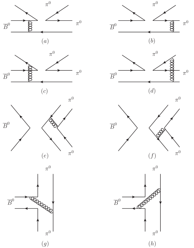
Figure 1: Typical Feynman diagrams contributing to the $\bar{B}^{0}\to\pi^{0}\pi^{0}$ decays in the PQCD approach at leading order.

In the PQCD, the soft ($\Phi$), hard ($H$), and harder ($C$) dynamics characterized by different scales make up the decay amplitude. It is conceptually written as follows:

$$Amplitude\sim\int d^{4}k_{1}d^{4}k_{2}d^{4}k_{3}Tr[C(t)\Phi_{\bar{B}^{0}}(k_{1})\Phi_{\pi^{0}}(k_{2})\Phi_{\pi^{0}}(k_{3})H(k_{1},k_{2},k_{3},t)],$$ (11)

where $k_{i}$ are the momenta of light quarks included in each meson, and $Tr$ denotes the trace over Dirac and color indices. The Wilson coefficient $C(t)$ results from the radiative corrections at short distance. The non-perturbative part is absorbed into wave function $\Phi_{M}$, which is universal and channel independent. $H$ describes the four quark operator and the quark pair produced by a gluon whose scale is at the order of $M_{B}$, so this hard part $H$ can be perturbative calculated.

We consider the $B$ meson at rest for simplicity and assume that the light final states poin meson moving along the direction of $n=(1,0,0_{T})$ and $v=(0,1,0_{T})$. It is convenient to use the light-cone coordinate $(P^{+},P^{-},P_{T})$ to describe the meson’s momenta, where, $P^{\pm}=\frac{1}{\sqrt{2}}(p^{0}\pm p^{3}),P_{T}=(p^{1},p^{2})$. Working at the rest frame of $\bar{B}^{0}$ meson, the momenta of $\bar{B}^{0}$, $\pi^{0}$, and $\pi^{0}$ can be written as follows:

$$P_{1}={M_{B}\over\sqrt{2}}(1,1,0_{T})\$$

$$P_{2}={M_{B}\over\sqrt{2}}(0,1,0_{T})\$$

$$P_{3}={M_{B}\over\sqrt{2}}(1,0,0_{T})$$ (12)

Putting the light (anti-) quark momenta in $\bar{B}^{0}$, $\pi^{0}$ and $\pi^{0}$ as $k_{1},k_{2},k_{3}$, respectively, we can choose:

$$k_{1}=(x_{1}p^{+}_{1},0,k_{1T})\$$

$$k_{2}=(0,x_{2}p^{-}_{2},k_{2T})\$$

$$k_{3}=(x_{3}p^{+}_{3},0,k_{3T})$$ (13)

Then, integrating over $k^{+}_{1},k^{-}_{2},k^{+}_{3}$ in Eq. (11) leads to

$$\begin{split}Amplitude\sim\int&d^{4}x_{1}d^{4}x_{2}d^{4}x_{3}b_{1}db_{1}b_{2}db_{2}b_{3}db_{3}\\ &\times Tr[C(t)\Phi_{\bar{B}^{0}}(x_{1},b_{1})\Phi_{\pi^{0}}(x_{2},b_{2})\Phi_{\pi^{0}}(x_{3},b_{3})H(x_{i},b_{i},t)]e^{-S(t)},\end{split}$$ (14)

where $b_{i}$ is the conjugate space coordinate of $k_{iT}$, and $t$ the largest energy scale in $H$. The exponential Sudakov factor $e^{-S(t)}$ comes from higher order radiative corrections to wave functions and hard amplitudes, it suppresses the soft dynamics effectively liTseng1998 and thus make a reliable perturbative calculation of the hard part $H$.

Fig. 1 shows the lowest order diagrams to be calculated in the PQCD approach for $\bar{B}^{0}\to\pi^{0}\pi^{0}$ decay. The sum contributions of the non-factorizable diagrams $(a)$ and $(b)$ which come from the operator $O_{2}$ are

$$\begin{split}{\cal M}_{a}=&\frac{-1}{\sqrt{2N_{c}}}32\pi C_{F}M_{B}^{2}\int_{0}^{1}dx_{1}dx_{2}dx_{3}\int_{0}^{\infty}b_{1}db_{1}b_{2}db_{2}\Phi_{B}(x_{1},b_{1})\{[(x_{2}-2)\Phi_{\pi}^{A}(x_{2})\Phi_{\pi}^{A}(x_{3})\\ &+r_{\pi}(1-2x_{2})\Phi_{\pi}^{T}(x_{2})\Phi_{\pi}^{A}(x_{3})+r_{\pi}(1-2x_{2})\Phi_{\pi}^{P}(x_{2})\Phi_{\pi}^{A}(x_{3})]\alpha_{s}(t_{a}^{1})h_{a}^{1}(x_{1},x_{2},x_{3},b_{1},b_{2})\\ &\exp[-S_{B}(t_{a}^{1})-S_{\pi}(t_{a}^{1})-S_{\pi}(t_{a}^{1})]C(t_{a}^{1})-2r_{\pi}\Phi_{\pi}^{P}(x_{2})\Phi_{\pi}^{A}(x_{3})\alpha_{s}(t_{a}^{2})\\ &h_{a}^{2}(x_{1},x_{2},x_{3},b_{1},b_{2})\exp[-S_{B}(t_{a}^{2})-S_{\pi}(t_{a}^{2})-S_{\pi}(t_{a}^{2})]C(t_{a}^{2})\},\end{split}$$ (15)

where $C_{F}=4/3$ is the group factor of the $SU(3)_{c}$ gauge group and $r_{\pi}=M_{0\pi}/M_{B}$. The wave function $\Phi_{M}$, the functions $h_{a}^{1,2}(x_{1},x_{2},x_{3},b_{1},b_{2})$, and the Sudakov factor $S_{X}(t_{i})(X=\bar{B}^{0},\pi^{0},\pi^{0})$ will be given in the appendix.

The total contribution for the non-factorizable diagrams $(c)$ and $(d)$ is

$$\begin{split}{\cal M}_{c}=&\frac{-1}{\sqrt{2N_{c}}}32\pi C_{F}M_{B}^{2}\int_{0}^{1}dx_{1}dx_{2}dx_{3}\int_{0}^{\infty}b_{2}db_{2}b_{3}db_{3}\Phi_{B}(x_{1},b_{3})\{[\Phi_{\pi}^{A}(x_{2})\Phi_{\pi}^{A}(x_{3})(1-x_{1}-x_{3})\\ &+r_{\pi}\Phi_{\pi}^{P}(x_{2})\Phi_{\pi}^{A}(x_{3})(1-x_{2})+r_{\pi}\Phi_{\pi}^{T}(x_{2})\Phi_{\pi}^{A}(x_{3})(1-x_{2})]\alpha_{s}(t_{c}^{1})h_{c}^{1}(x_{1},x_{2},x_{3},b_{2},b_{3})\\ &\exp[-S_{B}(t_{c}^{1})-S_{\pi}(t_{c}^{1})-S_{\pi}(t_{c}^{1})]C(t_{c}^{1})+[-\Phi_{\pi}^{A}(x_{2})\Phi_{\pi}^{A}(x_{3})(1+x_{3}-x_{1}-x_{2})-r_{\pi}\Phi_{\pi}^{P}(x_{2})\Phi_{\pi}^{A}(x_{3})(1-x_{2})\\ &+r_{\pi}\Phi_{\pi}^{T}(x_{2})\Phi_{\pi}^{A}(x_{3})(1-x_{2})]\alpha_{s}(t_{c}^{2})h_{c}^{2}(x_{1},x_{2},x_{3},b_{2},b_{3})\exp[-S_{B}(t_{c}^{2})-S_{\pi}(t_{c}^{2})-S_{\pi}(t_{c}^{2})]C(t_{c}^{2})\}.\end{split}$$ (16)

The factorizable annihilation diagrams $(e)$ and $(f)$ which come from the operators $O_{1},O_{3},O_{4},O_{5},O_{6},O_{7},O_{8},O_{9},O_{10}$ involve only two light mesons wave functions. $M_{e}$ is for $(V-A)(V-A)$ and $(V-A)(V+A)$ type operators, and $M_{e}^{p}$ is for $(1+\gamma_{5})(1-\gamma_{5})$ type operators:

$$\begin{split}{\cal M}_{e}=&8S\pi C_{F}M_{B}^{2}\int_{0}^{1}dx_{2}dx_{3}\int_{0}^{\infty}b_{2}db_{2}b_{3}db_{3}\{[-\Phi_{\pi}^{A}(x_{2})\Phi_{\pi}^{A}(x_{3})x_{2}-2r_{\pi}^{2}\Phi_{\pi}^{P}(x_{2})\Phi_{\pi}^{P}(x_{3})(1+x_{2})\\ &+2r_{\pi}^{2}\Phi_{\pi}^{T}(x_{2})\Phi_{\pi}^{P}(x_{3})(x_{2}-1)]\alpha_{s}(t_{e}^{1})h_{e}^{1}(x_{2},x_{3},b_{2},b_{3})\exp[-S_{\pi}(t_{e}^{1})-S_{\pi}(t_{e}^{1})]C(t_{e}^{1})\\ &+[\Phi_{\pi}^{A}(x_{2})\Phi_{\pi}^{A}(x_{3})x_{3}+2r_{\pi}^{2}\Phi_{\pi}^{P}(x_{2})\Phi_{\pi}^{P}(x_{3})(1+x_{3})+2r_{\pi}^{2}\Phi_{\pi}^{P}(x_{2})\Phi_{\pi}^{T}(x_{3})(1-x_{3})]\\ &\alpha_{s}(t_{e}^{2})h_{e}^{2}(x_{2},x_{3},b_{2},b_{3})\exp[-S_{\pi}(t_{e}^{2})-S_{\pi}(t_{e}^{2})]C(t_{e}^{2})\},\end{split}$$ (17)

$$\begin{split}{\cal M}_{e}^{P}=&8S\pi C_{F}M_{B}^{2}\int_{0}^{1}dx_{2}dx_{3}\int_{0}^{\infty}b_{2}db_{2}b_{3}db_{3}\{[-r_{\pi}\Phi_{\pi}^{P}(x_{2})\Phi_{\pi}^{A}(x_{3})x_{2}-r_{\pi}\Phi_{\pi}^{T}(x_{2})\Phi_{\pi}^{A}(x_{3})x_{2}\\ &-2r_{\pi}\Phi_{\pi}^{A}(x_{2})\Phi_{\pi}^{P}(x_{3})]\alpha_{s}(t_{e}^{1})h_{e}^{1}(x_{2},x_{3},b_{2},b_{3})\exp[-S_{\pi}(t_{e}^{1})-S_{\pi}(t_{e}^{1})]C(t_{e}^{1})+[-2r_{\pi}\Phi_{\pi}^{P}(x_{2})\Phi_{\pi}^{A}(x_{3})\\ &-r_{\pi}\Phi_{\pi}^{A}(x_{2})\Phi_{\pi}^{P}(x_{3})x_{3}-r_{\pi}\Phi_{\pi}^{A}(x_{2})\Phi_{\pi}^{T}(x_{3})x_{3}]\alpha_{s}(t_{e}^{2})h_{e}^{2}(x_{2},x_{3},b_{2},b_{3})\exp[-S_{\pi}(t_{e}^{2})-S_{\pi}(t_{e}^{2})]C(t_{e}^{2})\},\end{split}$$ (18)

where $S=2$ comes from the requirement of identity principle. The non-factorizable annihilation diagrams $(g)$ and $(h)$ come from the operators $O_{4},O_{6},O_{8},O_{10}$. $M_{g}$ is the contribution containing the operator of type $(V-A)(V-A)$, and $M_{g}^{P}$ is the contribution containing the operator of type $(1+\gamma_{5})(1-\gamma_{5})$.

$$\begin{split}{\cal M}_{g}=&\frac{1}{\sqrt{2N_{c}}}32S\pi C_{F}M_{B}^{2}\int_{0}^{1}dx_{1}dx_{2}dx_{3}\int_{0}^{\infty}b_{1}db_{1}b_{2}db_{2}\Phi_{B}(x_{1},b_{1})\{[(x_{1}+x_{3})\Phi_{\pi}^{A}(x_{2})\Phi_{\pi}^{A}(x_{3})\\ &+r_{\pi}^{2}(2+x_{1}+x_{2}+x_{3})\Phi_{\pi}^{P}(x_{2})\Phi_{\pi}^{P}(x_{3})-r_{\pi}^{2}\Phi_{\pi}^{P}(x_{2})\Phi_{\pi}^{T}(x_{3})(x_{2}-x_{1}-x_{3})+r_{\pi}^{2}\Phi_{\pi}^{T}(x_{2})\Phi_{\pi}^{P}(x_{3})(x_{1}+x_{3}-x_{2})\\ &-r_{\pi}^{2}\Phi_{\pi}^{T}(x_{2})\Phi_{\pi}^{T}(x_{3})(2-x_{1}-x_{2}-x_{3})]\alpha_{s}(t_{g}^{1})h_{g}^{1}(x_{1},x_{2},x_{3},b_{1},b_{2})\exp[-S_{B}(t_{g}^{1})-S_{\pi}(t_{g}^{1})-S_{\pi}(t_{g}^{1})]C(t_{g}^{1})\\ &+[-\Phi_{\pi}^{A}(x_{2})\Phi_{\pi}^{A}(x_{3})x_{2}+r_{\pi}^{2}\Phi_{\pi}^{P}(x_{2})\Phi_{\pi}^{P}(x_{3})(x_{1}-x_{2}-x_{3})-r_{\pi}^{2}\Phi_{\pi}^{P}(x_{2})\Phi_{\pi}^{T}(x_{3})(x_{1}-x_{3}+x_{2})\\ &-r_{\pi}^{2}\Phi_{\pi}^{T}(x_{2})\Phi_{\pi}^{P}(x_{3})(x_{1}-x_{3}+x_{2})+r_{\pi}^{2}\Phi_{\pi}^{T}(x_{2})\Phi_{\pi}^{T}(x_{3})(x_{1}-x_{2}-x_{3})]\alpha_{s}(t_{g}^{2})\\ &h_{g}^{2}(x_{1},x_{2},x_{3},b_{1},b_{2})\exp[-S_{B}(t_{g}^{2})-S_{\pi}(t_{g}^{2})-S_{\pi}(t_{g}^{2})]C(t_{g}^{2})\},\end{split}$$ (19)

$$\begin{split}{\cal M}_{g}^{P}=&\frac{-1}{\sqrt{2N_{c}}}32S\pi C_{F}M_{B}^{2}\int_{0}^{1}dx_{1}dx_{2}dx_{3}\int_{0}^{\infty}b_{1}db_{1}b_{2}db_{2}\Phi_{B}(x_{1},b_{1})\{[-\Phi_{\pi}^{A}(x_{2})\Phi_{\pi}^{A}(x_{3})x_{2}\\ &-r_{\pi}^{2}(2+x_{1}+x_{2}+x_{3})\Phi_{\pi}^{P}(x_{2})\Phi_{\pi}^{P}(x_{3})-r_{\pi}^{2}\Phi_{\pi}^{P}(x_{2})\Phi_{\pi}^{T}(x_{3})(x_{2}-x_{1}-x_{3})\\ &+r_{\pi}^{2}\Phi_{\pi}^{T}(x_{2})\Phi_{\pi}^{P}(x_{3})(x_{1}+x_{3}-x_{2})+r_{\pi}^{2}\Phi_{\pi}^{T}(x_{2})\Phi_{\pi}^{T}(x_{3})(x_{1}+x_{2}+x_{3}-2)]\alpha_{s}(t_{g}^{1})h_{g}^{1}(x_{1},x_{2},x_{3},b_{1},b_{2})\\ &\exp[-S_{B}(t_{g}^{1})-S_{\pi}(t_{g}^{1})-S_{\pi}(t_{g}^{1})]C(t_{g}^{1})+[-\Phi_{\pi}^{A}(x_{2})\Phi_{\pi}^{A}(x_{3})(x_{1}-x_{3})-r_{\pi}^{2}\Phi_{\pi}^{P}(x_{2})\Phi_{\pi}^{P}(x_{3})(x_{1}-x_{2}-x_{3})\\ &-r_{\pi}^{2}\Phi_{\pi}^{P}(x_{2})\Phi_{\pi}^{T}(x_{3})(x_{1}-x_{3}+x_{2})+r_{\pi}^{2}\Phi_{\pi}^{T}(x_{2})\Phi_{\pi}^{P}(x_{3})(x_{1}+x_{2}-x_{3})-r_{\pi}^{2}\Phi_{\pi}^{T}(x_{2})\Phi_{\pi}^{T}(x_{3})(x_{2}+x_{3}-x_{1})]\\ &\alpha_{s}(t_{g}^{2})h_{g}^{2}(x_{1},x_{2},x_{3},b_{1},b_{2})\exp[-S_{B}(t_{g}^{2})-S_{\pi}(t_{g}^{2})-S_{\pi}(t_{g}^{2})]C(t_{g}^{2})\},\end{split}$$ (20)

The total decay amplitude of $\bar{B}^{0}\to\pi^{0}\pi^{0}$ is then

$$\begin{split}{\cal\bar{A}}(\bar{B}^{0}\to\pi^{0}\pi^{0})=&V^{*}_{ud}V_{ub}[C_{1}{\cal M}_{\rm e}f_{B}+C_{2}({\cal M}_{\rm a}+{\cal M}_{\rm c})]-V^{*}_{td}V_{tb}[(2C_{3}+\frac{5}{3}C_{4}+2C_{5}+\frac{2}{3}C_{6}+\frac{1}{2}C_{7}\\ &+\frac{1}{6}C_{8}+\frac{1}{2}C_{9}-\frac{1}{3}C_{10}){\cal M}_{\rm e}f_{B}+(C_{6}-\frac{1}{2}C_{8}){\cal M}_{\rm e}^{\rm P}f_{B}+(2C_{4}+\frac{1}{2}C_{10}){\cal M}_{\rm g}+(2C_{6}+\frac{1}{2}C_{8}){\cal M}_{\rm g}^{\rm P}]\end{split}$$ (21)

and the decay width is expressed as

$$\Gamma(\bar{B}^{0}\to\pi^{0}\pi^{0})=\frac{G_{F}^{2}M_{B}^{3}}{128\pi}|{\cal\bar{A}}(\bar{B}^{0}\to\pi^{0}\pi^{0})|^{2}$$ (22)

The decay amplitude of the charge conjugate channel for $\bar{B}^{0}\to\pi^{0}\pi^{0}$ can be obtained by replacing $V^{*}_{ud}V_{ub}$ to $V_{ud}V^{*}_{ub}$ and $V^{*}_{td}V_{tb}$ to $V_{td}V^{*}_{tb}$ in Eq. (21). The decay amplitude of $\bar{B}^{0}\to\pi^{0}\pi^{0}$ in Eq. (21) can be parameterized as

$${\cal\bar{A}} = V^{*}_{ud}V_{ub}T-V^{*}_{td}V_{tb}P=V^{*}_{ud}V_{ub}T[1+ze^{i(-\alpha+\delta)}],$$ (23)

where $z=|V^{*}_{td}V_{tb}/V^{*}_{ud}V_{ub}||P/T|$, and $\delta=\arg(P/T)$ is the relative strong phase between tree diagrams $T$ and penguin diagrams $P$. $z$ and $\delta$ can be calculated from PQCD.

Similarly, the decay amplitude for $B^{0}\to\pi^{0}\pi^{0}$ can be parameterized as

$${\cal A} = V^{*}_{ub}V_{ud}T-V^{*}_{tb}V_{td}P=V^{*}_{ub}V_{ud}T[1+ze^{i(\alpha+\delta)}].$$ (24)

III Numerical Evaluation and discussions of results

The parameters have been used in numerical calculation Beringer2012 ; Amhis ; J.Charles:2005 ; A.Hocher:2001 ; H.-n.Li:2005 are shown in Table 1.

Table 1: The values of parameters adopted in numerical evaluation.

parameters	$\Lambda_{QCD}^{f=4}$	$m_{W}$	$m_{B}$	$f_{\pi}$	$f_{B}$	$m_{0\pi}$	$\tau_{B^{0}}$	$|V^{*}_{ud}V_{ub}|$	$|V^{*}_{td}V_{tb}|$
values	$\hskip 8.5359pt0.25$ GeV	$80.41$ GeV	$\hskip 8.5359pt5.280$ GeV	$\hskip 8.5359pt0.13$ GeV	$\hskip 8.5359pt0.21$ GeV	$\hskip 8.5359pt1.4$ GeV	$\hskip 8.5359pt1.55\times 10^{-12}$ s	$\hskip 8.5359pt0.00346$	$\hskip 8.5359pt0.00885$

We leave the Cabibbo-Kobayashi-Maskawa (CKM) phase angle $\alpha$ as a free parameter to explore the branching ratio and CP asymmetry. From Eqs. (23) and (24), we get the averaged decay width for $\bar{B}^{0}(B^{0})\to\pi^{0}\pi^{0}$

$$\Gamma(\bar{B}^{0}(B^{0})\to\pi^{0}\pi^{0}) = \frac{G_{F}^{2}M_{B}^{3}}{128\pi}(\frac{|{\cal A}|^{2}}{2}+\frac{|{\cal\bar{A}}|^{2}}{2})$$ (25)

$$= \frac{G_{F}^{2}M_{B}^{3}}{128\pi}|V^{*}_{ud}V_{ub}T|^{2}[1+2z\cos(\alpha)\cos(\delta)+z^{2}].$$

Using the above parameters, we get $z=0.52$ and $\delta=106^{\circ}$ in PQCD. Equation (25) is a function of CKM angle $\alpha$. In Fig. 2, we plot the averaged branching ratio of the decay $\bar{B}^{0}(B^{0})\to\pi^{0}\pi^{0}$ with respect to the parameter $\alpha$. Since the CKM angle $\alpha$ is constrained as $\alpha$ around $85^{\circ}$ A.Hocher:2001 .

$$\alpha=(85.4_{-3.8}^{+3.9})^{\circ}$$ (26)

We can arrive from Fig. 2

$$1.15\times 10^{-6}<Br(\bar{B}^{0}(B^{0})\to\pi^{0}\pi^{0})<1.18\times 10^{-6},\hskip 14.22636ptfor80^{\circ}<\alpha<90^{\circ}$$ (27)

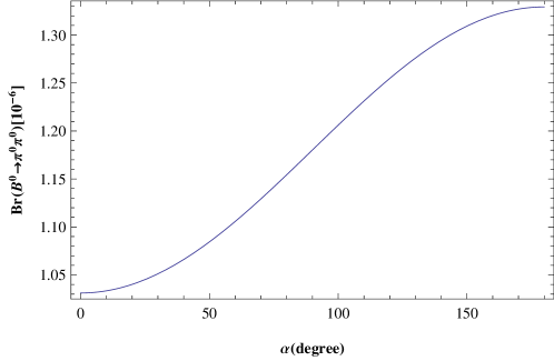
Figure 2: The averaged branching ratio of $\bar{B}^{0}(B^{0})\to\pi^{0}\pi^{0}$ decay as a function of CKM angle $\alpha$.

The number $z=|V^{*}_{td}V_{tb}/V^{*}_{ud}V_{ub}||P/T|=0.52$ means that the amplitude of penguin diagrams is about 0.52 times that of tree diagrams, which shows though the tree contribution dominate this decay, the penguin contribution cannot be ignored, i. e., there are large contributions from both tree diagrams and penguin diagrams.

Besides the phase angle $\alpha$, the major theoretical errors come from the uncertainties of $\omega_{b}=0.4\pm 0.04$ GeV, $f_{B}=0.21\pm 0.02$ GeV, and the Gegenbauer moment $a_{2}^{\pi}=0.25\pm 0.15$. Taking into account the uncertainties of these parameters, we find

$$Br(\bar{B}^{0}(B^{0})\to\pi^{0}\pi^{0})=\left[1.17_{-0.08}^{+0.09}(\omega_{b})_{-0.07}^{+0.05}(f_{B})_{-0.06}^{+0.02}(a_{2}^{\pi})\right]\times 10^{-6}.$$ (28)

When all important theoretical errors from different sources, including those from the uncertainty of phase angle $\alpha$, are added in quadrature, we get $Br(\bar{B}^{0}(B^{0})\to\pi^{0}\pi^{0})=(1.17_{-0.12}^{+0.11})\times 10^{-6}$.

In the literature, there already exist a lot of studies on $B^{0}\rightarrow\pi^{0}\pi^{0}$ decay. We give some recent works devoted to the resolution of the challenge:

(a) In Ref. QChang2014 , Qin Chang and Junfeng Sun $et$ $al$ do a global fit on the spectator scattering and annihilation parameters$X_{H}(\rho_{H},\phi_{H})$, $X_{A}^{i}(\rho_{A}^{i},\phi_{A}^{i})$ and $X_{A}^{f}(\rho_{A}^{f},\phi_{A}^{f})$ for the available experimental data for $B_{u,d}\rightarrow\pi\pi,\pi K$ and $K\bar{K}$ decays in the QCDF framework. They obtained large ${B}^{0}\to\pi^{0}\pi^{0}$ branching ratios $(1.67_{-0.30}^{+0.33})\times 10^{-6}$ and $(2.13_{-0.38}^{+0.43})\times 10^{-6}$ for different scenarios.

(b)In Ref. XLiu2015 , Xin Liu , Hsiang-nan Li and Zhen-Jun Xiao investigate the Glauber-gluon effect on the $B\rightarrow\pi\pi$ and $\rho\rho$ decays based on the $k_{T}$ factorization theorem, they observed significant modification of $B^{0}\rightarrow\pi^{0}\pi^{0}$ branching ratio through a transverse-momentum-dependent(TMD) wave function for the pion with a weak falloff in parton transverse momentum $k_{T}$. They get the branching ratio of $B^{0}\rightarrow\pi^{0}\pi^{0}$ $0.61\times 10^{-6}$.

(c)In Ref. CFQiao2015 , Cong-Feng Qiao $et$ $al$ give a possible solution to the $B\rightarrow\pi\pi$ puzzle using the Principle of Maximum Conformality(PMC). They applied the PMC procedure to the QCDF analysis with the goal of eliminating the renormalization scale ambiguity and achieving an accurate pQCD prediction which is independent of theoretical conventions. They found the pQCD prediction is highly sensitive to the choice of the renormalization scale which enter the decay amplitude, they obtained $Br(B_{d}\rightarrow\pi^{0}\pi^{0})=(0.98^{+0.44}_{-0.31})\times 10^{-6}$ by applying the principle of maximum conformality. However, we find the PQCD prediction is not sensitive to the choice of the renormalization scale for this decay based on our calculation. In our approach, we set the renormalization scale $\mu=t$(the largest energy scale in $H$) to diminish the large logarithmic radiative corrections and minimize the NLO contributions to the form factors. By changing the hard scale $t$ from $0.9t$ to $1.3t$, we find the branching ratio of $B^{0}\rightarrow\pi^{0}\pi^{0}$ change a little. The choice of the renormalization scale is not a main reason for the $B^{0}\rightarrow\pi^{0}\pi^{0}$ puzzle, even when the NLO contributions are taken into account Ya-Lan Zhang:2015 .

(d)In Ref. Ya-Lan Zhang:2015 , Ya-Lan Zhang $et$ $al$ performed a systematic study for the $B\rightarrow(\pi^{+}\pi^{-},\pi^{+}\pi^{0},\pi^{0}\pi^{0})$ decays in the PQCD factorization approach with the inclusion of all currently known NLO contributions from various sources. They got the NLO PQCD prediction for $B^{0}\rightarrow\pi^{0}\pi^{0}$ branching ratio $Br(B^{0}\rightarrow\pi^{0}\pi^{0})=[0.23_{-0.05}^{+0.08}(\omega(b))_{-0.04}^{+0.05}(f_{B})_{-0.03}^{+0.04}(a_{2}^{\pi})]\times 10^{-6}$, it is still much smaller than the measured data.

(e)In Ref. H.Y.Cheng:2015 , Hai-Yang Cheng, Cheng-Wei Chiang and An-Li Kuo used flavor SU(3) symmetry to analyze the data of charmless $B$ meson decays to two pseudoscalar mesons $(PP)$ and one vector and one pseudoscalar mesons $(VP)$ . They found the color-suppressed tree amplitude larger than previously known and has a strong phase of $-70^{\circ}$ relative to the color favored tree amplitude in the PP sector, this large color-suppressed tree amplitude results in the large $B^{0}\rightarrow\pi^{0}\pi^{0}$ branching ratios $1.43\pm 0.55\times 10^{-6}$ and $1.88\pm 0.42\times 10^{-6}$ for different scheme.

Table 2: The pQCD predictions for the CP-averaged branching ratios(in unit of $10^{-6}$).

Channel	LO LUY	NLO H.-n.Li:2005	NLO Ya-Lan Zhang:2015	LO(this work)	QCDF Beneke2003	BABAR Data Heavy	Belle Data Heavy	HFAG Data  Heavy
$B^{0}\rightarrow\pi^{0}\pi^{0}$	$0.12$	$0.29$	$0.23$	$1.17_{-0.12}^{+0.11}$	$0.3$	$1.83\pm 0.21\pm 0.13$	$0.90\pm 0.12\pm 0.10$	$1.17\pm 0.13$

There are some works on $B^{0}\rightarrow\pi^{0}\pi^{0}$ decay in the framework of PQCD approach beforeLUY ; H.-n.Li:2005 ; Ya-Lan Zhang:2015 , we list these numerical values in Table 2. Ref. LUY is the earliest PQCD calculations for $B^{0}\rightarrow\pi^{0}\pi^{0}$ decay at the leading order(LO), Hsiang-nan Li $et$ $al$ considered partial NLO contributions in Ref. H.-n.Li:2005 . Based on the work of Refs. LUY ; H.-n.Li:2005 , Ya-Lan Zhang $et$ $al$ calculated all currently known NLO contributions from various sources in Ref. Ya-Lan Zhang:2015 . As shown in Table 2, one can see that the NLO contributions are much larger than LO contributions for $B^{0}\rightarrow\pi^{0}\pi^{0}$ decay in previous works. Despite this, it is still much smaller than the experimental data. In this work, we recalculate the $B^{0}\rightarrow\pi^{0}\pi^{0}$ decay in the framework of PQCD approach at LO. Our result is much larger than that of previous predictionsLUY ; H.-n.Li:2005 ; Ya-Lan Zhang:2015 , there are two reasons that make the difference. For the operator $O_{1}=(\bar{u}_{\alpha}u_{\alpha})_{V-A}(\bar{d}_{\beta}b_{\beta})_{V-A}$, it can contribute not only to non-factorizable diagrams (a) and (b), but to factorizable annihilation diagrams (e) and (f)(see Fig. 1) as well. We find the largest contributions come from the factorizable annihilation diagrams $(e)$ and $(f)$, which come from tree operator $O_{1}$ and penguin operators $O_{3},O_{4},O_{5},O_{6},O_{7},O_{8},O_{9},O_{10}$. In previous PQCD worksLUY ; H.-n.Li:2005 ; Ya-Lan Zhang:2015 , first, the contributions of the factorizable annihilation diagrams $(e)$ and $(f)$ come from tree operator $O_{1}$ had not been taken into account, the authors only considered the non-factorizable diagrams $(a)$ and $(b)$(small contributions) for operator $O_{1}$; second, For $O_{3},O_{4},O_{9},O_{10}$ operators, previous calculationsLUY showed their contributions cancel between diagrams $(e)$ and $(f)$, however, we recalculate it and find their contributions cannot be canceled between diagrams $(e)$ and $(f)$, as shown in Eqs.(17)(18). If we get rid of the contributions of ${\cal M}_{\rm e}$ and ${\cal M}_{\rm e}^{\rm P}$ terms in Eq. (21), our result is $Br(\bar{B}^{0}(B^{0})\to\pi^{0}\pi^{0})\sim 0.26\times 10^{-6}$, which is consistent with previous PQCD predictionsLUY ; H.-n.Li:2005 ; Ya-Lan Zhang:2015 . The hard scale $t$ in Eq. (14) characterizes the size of NLO contributions, by changing the hard scale $t$ from $0.9t$ to $1.3t$, we find the branching ratio of $B^{0}\rightarrow\pi^{0}\pi^{0}$ changes about $~{}10\%$, which means although the NLO diagrams may make a significant contributions to $B^{0}\rightarrow\pi^{0}\pi^{0}$ decayH.-n.Li:2005 ; Ya-Lan Zhang:2015 , the LO contributions still dominate this decay. Because there are identical particles in final state for this decay, one must consider identical principle. Usually the decay width receives a symmetry factor $1/2$ due to the identical particles in the final state, but in our calculations, we have calculated the symmetrized Feynman diagrams and all these contributions have been included in the total decay amplitude formula(21), and hence there is no need to add an extra factor in decay width. In our recalculations, we consider all the possible diagrams’s contribution, including non-factorizable contributions and annihilation contributions. We obtain the branching ratio of $B^{0}\to\pi^{0}\pi^{0}$ $(1.17_{-0.12}^{+0.11})\times 10^{-6}$, which is still smaller than BABAR result Heavy , but it is consistent with the Belle and HFAG results Heavy . More experimental and theoretical efforts should be made to resolve the $B^{0}\rightarrow\pi^{0}\pi^{0}$ puzzle.

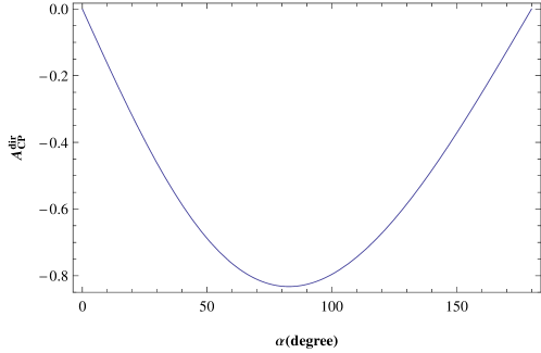
Figure 3: Direct CP violation parameter of $\bar{B}^{0}(B^{0})\to\pi^{0}\pi^{0}$ decay as a function of CKM angle $\alpha$.

In SM , the CKM phase angle is the origin of CP violation. Using Eqs.(23) and (24), the direct CP violating parameter is

$${\cal A}_{CP}^{\rm dir} = \frac{|\cal\bar{A}|^{\rm 2}-|\cal A|^{\rm 2}}{|\cal\bar{A}|^{\rm 2}+|\cal A|^{\rm 2}}=\frac{2z\sin(\alpha)\sin(\delta)}{1+2z\cos(\alpha)\cos(\delta)+z^{2}}$$ (29)

It is approximately proportional to CKM angle $\sin(\alpha)$, strong phase $\sin(\delta)$, and the relative size $z$ between penguin contribution and tree contribution. We show the direct CP asymmetry ${\cal A}_{CP}^{\rm dir}$ in Fig. 3. One can see from this figure that the direct CP asymmetry parameter of $\bar{B}^{0}(B^{0})\to\pi^{0}\pi^{0}$ can be as large as from $-83\%$ to $-82\%$ when $80^{\circ}<\alpha<90^{\circ}$. The large direct CP asymmetry is also a result of there are large contributions from both tree diagrams and penguin diagrams in this decays.

For the neutral $B^{0}$ decays, the $\bar{B}^{0}-B^{0}$ mixing is very complex. Following notations in the previous literature  G.Kramer:1997 , we define the mixing induced CP violation parameter as

$$a_{\epsilon+\epsilon^{\prime}}=\frac{-2Im(\lambda_{CP})}{1+|\lambda_{CP}|^{2}},$$ (30)

where

$$\lambda_{CP}=\frac{V^{*}_{tb}V_{td}<\pi^{0}\pi^{0}|H_{eff}|\bar{B}^{0}>}{V_{tb}V^{*}_{td}<\pi^{0}\pi^{0}|H_{eff}|B^{0}>}.$$ (31)

Using equations (23) and (24), we can derive as

$$\lambda_{CP}=e^{2i\alpha}\frac{1+ze^{i(\delta-\alpha)}}{1+ze^{i(\delta+\alpha)}}$$ (32)

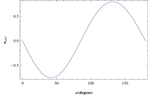
Figure 4: Mixing CP violation parameter of $\bar{B}^{0}(B^{0})\to\pi^{0}\pi^{0}$ decay as a function of CKM angle $\alpha$.

If $z$ is a very small number, i. e., the penguin diagram contribution is suppressed comparing with the tree diagram contribution, the mixing induced CP asymmetry parameter $a_{\epsilon+\epsilon^{\prime}}$ is proportional to $-\sin 2\alpha$, which will be a good place for the CKM angle $\alpha$ measurement. However as we have already mentioned, $z$ is not very small. We give the mixing CP asymmetry in Fig. 4, one can see that $a_{\epsilon+\epsilon^{\prime}}$ is not a simple $-\sin 2\alpha$ behavior because of the so-called penguin pollution. It is close to $6\%$ when the angle near $85^{\circ}$. At present, there are no CP asymmetry measurements in experiment but the possible large CP violation we predict for $\bar{B}^{0}(B^{0})\to\pi^{0}\pi^{0}$ decays might be observed in the coming Belle-II experiments.

IV Summary

In this work, we recalculate the branching ratio and CP asymmetries of the decays $\bar{B}^{0}(B^{0})\to\pi^{0}\pi^{0}$ in PQCD approach at LO. From our calculations, we find the branching ratio of $B^{0}\to\pi^{0}\pi^{0}$ $(1.17_{-0.12}^{+0.11})\times 10^{-6}$, much larger than that of previous predictionsLUY , and there are large CP violation in this process, which may be measured in the coming Belle-II experiments. The branching ratio we get is still smaller than BABAR result Heavy , but it is consistent with the latest Belle and HFAG results Heavy .

V Appendix : Formulae For The Calculations Used In The Text

We present the explicit expressions of the formulae used in Sec. II in the appendix. The expressions of the meson distribution amplitudes $\Phi_{M}$ are given at first. For $B^{0}$ meson wave function, we use the function LUY ; Keum2001 ; Y.-Y.Keum:2001

$$\phi_{B}(x,b) = N_{B}x^{2}(1-x)^{2}\exp\left[-\frac{1}{2}\left(\frac{xm_{B}}{\omega_{b}}\right)^{2}-\frac{\omega_{b}^{2}b^{2}}{2}\right]\;,$$ (33)

The parameter $\omega_{b}=0.4$ GeV is constrained by other charmless $B$ decays LUY ; Keum2001 ; Y.-Y.Keum:2001 . For the $\pi$ meson’s wave function, the distribution amplitude $\Phi_{\pi}^{A}$ for the twist-2 wave function and the distribution amplitude $\Phi_{\pi}^{P}$ and $\Phi_{\pi}^{T}$ of the twist-3 wave functions are taken from  H.-n.Li:2005 ; Z.J.Xiao:2008 ; Y.Y.Fan:2013 ; Z.J.Xiao:2012

$$\Phi_{\pi}^{A}(x) = \frac{3f_{\pi}}{\sqrt{2N_{c}}}x(1-x)\times[1+a_{1}^{\pi}C_{1}^{\frac{3}{2}}(2x-1)+a_{2}^{\pi}C_{2}^{\frac{3}{2}}(2x-1)+a_{4}^{\pi}C_{4}^{\frac{3}{2}}(2x-1)];$$

$$\Phi_{\pi}^{P}(x) = \frac{f_{\pi}}{2\sqrt{2N_{c}}}\left[1+(30\eta_{3}-\frac{5}{2}\rho_{\pi}^{2})C_{2}^{\frac{1}{2}}(2x-1)-3\{\eta_{3}\omega_{3}+\frac{9}{20}\rho_{\pi}^{2}(1+6a_{2}^{\pi})\}C_{4}^{\frac{1}{2}}(2x-1)\right];$$

$$\Phi_{\pi}^{T}(x) = \frac{f_{\pi}}{2\sqrt{2N_{c}}}(1-2x)\left[1+6\left(5\eta_{3}-\frac{1}{2}\eta_{3}\omega_{3}-\frac{7}{20}\rho_{\pi}^{2}-\frac{3}{5}\rho_{\pi}^{2}a_{2}^{\pi}\right)(1-10x+10x^{2})\right],$$ (34)

where $a_{i}^{\pi}$ are the Gegenbauer moments, the mass ratio $\rho_{\pi}=m_{\pi}/m_{0\pi}$. The Gegenbauer polynomials are defined by  H.-n.Li:2005 .

$$C_{2}^{\frac{1}{2}}(t) = \frac{1}{2}(3t^{2}-1);$$

$$C_{4}^{\frac{1}{2}}(t) = \frac{1}{8}(35t^{4}-30t^{2}+3);$$

$$C_{2}^{\frac{3}{2}}(t) = \frac{3}{2}(5t^{2}-1);$$

$$C_{4}^{\frac{3}{2}}(t) = \frac{15}{8}(21t^{4}-14t^{2}+1);$$

$$C_{1}^{\frac{3}{2}}(t) = 3t,$$ (35)

and the Gegenbauer moments and other parameters are adopted from Refs.H.-n.Li:2005 ; P.Ball:2005

$$a_{1}^{\pi}=0, \quad a_{2}^{\pi}=0.25, \quad a_{4}^{\pi}=-0.015,$$

$$\rho_{\pi}=m_{\pi}/m_{0\pi}, \quad\eta_{3}=0.015, \quad\omega_{3}=-3.0$$ (36)

with $m_{0\pi}$ the chiral mass of the pion.

$S_{\bar{B}^{0}}$, $S_{\pi^{0}}$, $S_{\pi^{0}}$ used in the decay amplitudes are defined as

$$S_{\bar{B}^{0}}(t) = s(x_{1}P_{1}^{+},b_{1})+2\int_{\frac{1}{b_{1}}}^{t}\frac{d\bar{\mu}}{\bar{\mu}}\gamma(\alpha_{s}(\bar{\mu})),$$ (37)

$$S_{\pi^{0}}(t) = s(x_{2}P_{2}^{-},b_{2})+s((1-x_{2})P_{2}^{-},b_{2})+2\int_{\frac{1}{b_{2}}}^{t}\frac{d\bar{\mu}}{\bar{\mu}}\gamma(\alpha_{s}(\bar{\mu})),$$ (38)

$$S_{\pi^{0}}(t) = s(x_{3}P_{3}^{+},b_{3})+s((1-x_{3})P_{3}^{+},b_{3})+2\int_{\frac{1}{b_{3}}}^{t}\frac{d\bar{\mu}}{\bar{\mu}}\gamma(\alpha_{s}(\bar{\mu})),$$ (39)

where the so called Sudakov factor $s(Q,b)$ resulting from the resummation of double logarithms is given as  H.-n.Li:2003 ; H.-n.Li:1999

$$s(Q,b)=\int_{\frac{1}{b}}^{Q}\frac{d\mu}{\mu}\left[\ln(\frac{Q}{\mu})A(\alpha(\bar{\mu}))+B(\alpha_{s}(\bar{\mu}))\right]$$ (40)

with

$$A = C_{F}\frac{\alpha_{s}}{\pi}+\left[\frac{67}{9}-\frac{\pi^{2}}{3}-\frac{10}{27}n_{f}+\frac{2}{3}\beta_{0}\ln(\frac{e^{\gamma_{E}}}{2})\right](\frac{\alpha_{s}}{\pi})^{2},$$ (41)

$$B = \frac{2}{3}\frac{\alpha_{s}}{\pi}\ln\left(\frac{e^{2\gamma_{E}-1}}{2}\right),$$ (42)

here $\gamma_{E}=0.57722\cdot\cdot\cdot$ is the Euler constant, $n_{f}$ is the active quark flavor number.

The functions $h_{i}(i=a,c,e,g)$ come from the Fourier transformation of propagators of virtual quark and gloun in the hard part calculations. They are given as follow

$$h_{a}^{j}(x_{1},x_{2},x_{3},b_{1},b_{2})=$$

$$\biggl{\{}\theta(b_{1}-b_{2})I_{0}(M_{B}\sqrt{x_{1}(1-x_{2})}b_{2})K_{0}(M_{B}\sqrt{x_{1}(1-x_{2})}b_{1})$$

$$\qquad\qquad\qquad\qquad+(b_{1}\leftrightarrow b_{2})\biggr{\}}\times\left(\begin{matrix}\mathrm{(}K_{0}(M_{B}F_{a(j)}b_{1}),&\text{for}\quad F^{2}_{a(j)}>0\\ \frac{\pi i}{2}\mathrm{H}_{0}^{(1)}(M_{B}\sqrt{|F_{a(j)}^{2}|}b_{1}),&\text{for}\quad F^{2}_{a(j)}<0\end{matrix}\right),$$ (43)

where $F_{a(j)}$’s are defined by

$$F_{a(1)}^{2}=1-x_{2}\ ,$$

$$F_{a(2)}^{2}=x_{1}\;.$$ (44)

$$h_{c}^{j}(x_{1},x_{2},x_{3},b_{2},b_{3})=$$

$$\biggl{\{}\theta(b_{2}-b_{3})I_{0}(M_{B}\sqrt{x_{1}(1-x_{2})}b_{3})K_{0}(M_{B}\sqrt{x_{1}(1-x_{2})}b_{2})$$

$$\qquad\qquad\qquad\qquad+(b_{2}\leftrightarrow b_{3})\biggr{\}}\times\left(\begin{matrix}\mathrm{(}K_{0}(M_{B}F_{c(j)}b_{3}),&\text{for}\quad F^{2}_{c(j)}>0\\ \frac{\pi i}{2}\mathrm{H}_{0}^{(1)}(M_{B}\sqrt{|F_{c(j)}^{2}|}b_{3}),&\text{for}\quad F^{2}_{c(j)}<0\end{matrix}\right),$$ (45)

where $F_{c(j)}$’s are defined by

$$F_{c(1)}^{2}=x_{1}+x_{2}+x_{3}-x_{1}x_{2}-x_{2}x_{3}-1\ ,$$

$$F_{c(2)}^{2}=x_{1}-x_{3}-x_{1}x_{2}+x_{2}x_{3}\;.$$ (46)

$$h_{e}^{1}(x_{2},x_{3},b_{2},b_{3})= S_{t}(x_{2})K_{0}(M_{B}\sqrt{x_{2}x_{3}}b_{3})$$ (47)

$$\times\{\theta(b_{2}-b_{3})I_{0}(M_{B}\sqrt{x_{2}}b_{2})K_{0}(M_{B}\sqrt{x_{2}}b_{3})+(b_{2}\leftrightarrow b_{3})\},$$

$$h_{e}^{2}(x_{2},x_{3},b_{2},b_{3})= S_{t}(x_{3})K_{0}(M_{B}\sqrt{x_{2}x_{3}}b_{2})$$ (48)

$$\times\{\theta(b_{2}-b_{3})I_{0}(M_{B}\sqrt{x_{3}}b_{3})K_{0}(M_{B}\sqrt{x_{3}}b_{2})+(b_{2}\leftrightarrow b_{3})\}.$$

$$h_{g}^{j}(x_{1},x_{2},x_{3},b_{1},b_{2})=$$

$$\biggl{\{}\theta(b_{1}-b_{2})I_{0}(M_{B}\sqrt{x_{2}x_{3}}b_{1})K_{0}(M_{B}\sqrt{x_{2}x_{3}}b_{2})$$

$$\qquad\qquad\qquad\qquad+(b_{1}\leftrightarrow b_{2})\biggr{\}}\times\left(\begin{matrix}\mathrm{(}K_{0}(M_{B}F_{g(j)}b_{1}),&\text{for}\quad F^{2}_{g(j)}>0\\ \frac{\pi i}{2}\mathrm{H}_{0}^{(1)}(M_{B}\sqrt{|F_{g(j)}^{2}|}b_{1}),&\text{for}\quad F^{2}_{g(j)}<0\end{matrix}\right),$$ (49)

where $F_{g(j)}$’s are defined by

$$F_{g(1)}^{2}=x_{1}+x_{2}+x_{3}-x_{1}x_{2}-x_{2}x_{3}\ ,$$

$$F_{g(2)}^{2}=x_{1}x_{2}-x_{2}x_{3}\;.$$ (50)

We adopt the parametrization for $S_{t}(x)$ contributing to the factorizable diagrams  T.Kurimoto:2003

$$S_{t}(x)=\frac{2^{1+2c}\Gamma(\frac{3}{2}+c)}{\sqrt{\pi}\Gamma(1+c)}[x(1-x)]^{c}$$ (51)

where the parameter $c=0.3$. The hard scale $t$ in the amplitudes are taken as the largest energy scale in $H$ to kill the large logarithmic radiative corrections:

$$\begin{split}&t_{a}^{1}=\max(M_{B}\sqrt{\mid F_{a(1)}^{2}\mid},M_{B}\sqrt{x_{1}(1-x_{2})},\frac{1}{b_{1}},\frac{1}{b_{2}})\;;\\ \\ &t_{a}^{2}=\max(M_{B}\sqrt{\mid F_{a(2)}^{2}\mid},M_{B}\sqrt{x_{1}(1-x_{2})},\frac{1}{b_{1}},\frac{1}{b_{2}})\;;\\ \\ &t_{c}^{1}=\max(M_{B}\sqrt{\mid F_{c(1)}^{2}\mid},M_{B}\sqrt{x_{1}(1-x_{2})},\frac{1}{b_{2}},\frac{1}{b_{3}})\;;\\ \\ &t_{c}^{2}=\max(M_{B}\sqrt{\mid F_{c(2)}^{2}\mid},M_{B}\sqrt{x_{1}(1-x_{2})},\frac{1}{b_{2}},\frac{1}{b_{3}})\;;\\ \\ &t_{e}^{1}=\max(M_{B}\sqrt{x_{2}},\frac{1}{b_{2}},\frac{1}{b_{3}})\;;\\ \\ &t_{e}^{2}=\max(M_{B}\sqrt{x_{3}},\frac{1}{b_{2}},\frac{1}{b_{3}})\;;\\ \\ &t_{g}^{1}=\max(M_{B}\sqrt{\mid F_{g(1)}^{2}\mid},M_{B}\sqrt{x_{2}x_{3}},\frac{1}{b_{1}},\frac{1}{b_{2}})\;;\\ &t_{g}^{2}=\max(M_{B}\sqrt{\mid F_{g(2)}^{2}}\mid,M_{B}\sqrt{x_{2}x_{3}},\frac{1}{b_{1}},\frac{1}{b_{2}}).\end{split}$$

References

• (1) J.Beringer $et$ $al$. [Particle Data Group Collaboration], Phys. Rev. D 86, 010001 (2012) and 2013 partial update for the 2014 edition.
• (2) Y. Amhis $et$ $al$. [Heavy Flavor Averaging Group Collab-oration], arXiv:1207.1158.
• (3) B. Aubert $et$ $al$. [BaBar Collaboration], Phys. Rev. Lett. 91(24), 241801 (2003); Phys.  Rev. Lett.  94(18), 181802(2005); K. Abe $et$ $al$. [Belle Collaboration], Phys. Rev. Lett.  94(18), 181803(2005).
• (4) M.Beneke, T. Huber and X. Q. Li, Nucl. Phys. B 832, 109(2010); G. Bell, Nucl. Phys. B 822, 172(2009); V. Pilipp, Nucl. Phys. B794, 154(2008); G. Bell, Nucl. Phys. B 795, 1(2008).
• (5) M.Beneke and M. Neubert, Nucl. Phys. B 675, 333(2003).
• (6) C. N. Burrell and A. R. Williamson, Phys. Rev. D 73, 114004(2006).
• (7) M. Beneke and D. Yang, Nucl. Phys. B736,34(2006); M. Beneke and S. Jäger, Nucl. Phys. B 751, 160(2006).
• (8) Cai-Dian Lü, Kazumasa Ukai, Mao-Zhi Yang, Phys. Rev. D 63(7), 074009 (2001).
• (9) M.Wirble, B.Stech, and M.Bauer, Z. Phys. C 29, 637 (1985), 34, 103 (1987); M. Bauer and M. Wirbel, Z. Phys. C 42, 671(1989); L.-L.Chau, H.-Y.Cheng, W.K.Sze, H.Yao, and B.Tseng, Phys. Rev. D 43(7), 2176(1991).
• (10) A.Ali, G.Kramer, and C.D.Lü, Phys. Rev. D 58(9), 094009(1998).
• (11) Y.H.Chen, H.Y.Cheng, B.Tseng, and K.C.Yang, Phys. Rev. D 60(9), 094014 (1999).
• (12) M.Beneke, G.Buchalla, M.Neubert, and C.T.Sachrajda, Nucl. Phys. B 591(1), 313 (2000); Phys. Rev. Lett.  83(10), 1914 (1999).
• (13) H.n.Li and H.L.Yu, Phys. Rev. Lett.  74(22), 4388 (1995); Phys. Lett. B 353(2), 301 (1995); H.-n.Li and H.L.Yu, Phys. Rev. D 53(5),2480 (1996).
• (14) Y.Y.Keum, H.-n.Li and A.I.Sanda, Phys. Rev. D 63(5), 054008 (2001).
• (15) Heavy Flavor Averaging Group, Y. Amhis $et$ $al$. arXiv:1412.7515.
• (16) Q. Chang, J. Sun, Y. Yang, and X. Li, Phys. Rev. D 90(5), 054019 (2014).
• (17) Xin.Liu, Hsiang-nan.Li, Zhen-Jun.Xiao, Phys. Rev. D 91, 114019 (2015).
• (18) C. F. Qiao, R. L. Zhu, X. G. Wu and S. J. Brodsky, Phys. Lett. B 748, 422 (2015).
• (19) S.Nandi and H.-n. Li, Phys. Rev. D 76(3), 034008 (2007).
• (20) H.-n. Li, Y.L. Shen, Y.M. Wang and H.Zou, Phys. Rev. D 83(5), 054029 (2011).
• (21) H.-n. Li, Y.L. Shen, Y.M. Wang, Phys. Rev. D 85(7), 074004 (2012).
• (22) H.-n. Li and S. Mishima, Phys. Rev. D 73(11), 114014 (2006).
• (23) G.Buchalla, A.J.Buras and M.E.Lautenbacher, Rev. Mod.  Phys. 68(4), 1125 (1996).
• (24) H.-n. Li and B. Tseng, Phys. Rev. D 57, 443(1998).
• (25) J.Charles $et$ $al$.[CKMfitter Group], Eur. Phys. J. C 41(1), 1 (2005).
• (26) A.Höcker $et$ $al$, Eur. Phys. J. C 21(2), 225 (2001).
• (27) H.-n.Li, S.Mishima, and A.I.Sanda, Phys. Rev. D 72, 114005 (2005).
• (28) Ya-Lan Zhang, Xue-Yan Liu, Ying-Ying Fan, Shan Cheng, and Zhen-Jun Xiao, Phys. Rev. D 90(1), 014029 (2014).
• (29) H.Y.Cheng, C.W.Chiang, and A.L.Kuo, Phys. Rev. D 91(1), 014011 (2015).
• (30) G.Kramer, W.F.Palmer, and Y.L.Wu, Communications in Theoretical Physics. 27(4), 457 (1997).
• (31) Y.-Y.Keum, H.-n.Li, and A.I.Sanda, Phys. Lett. B 504(1), 6 (2001).
• (32) Z.J.Xiao, Z.Q.Zhang, X.Liu, and L.B.Guo, Phys. Rev. D 78, 114001 (2008).
• (33) Y.Y.Fan, W.F.Wang, S.Cheng, and Z.J.Xiao, Phys. Rev. D 87, 094003 (2013).
• (34) Z.J.Xiao, W.F.Wang, and Y.Y.Fan, Phys. Rev. D 85, 094003 (2012); W.F.Wang and Z.J.Xiao, Phys. Rev. D 86, 114025 (2012).
• (35) P.Ball and R.Zwicky, Phys. Rev. D 71, 014015 (2005).
• (36) H.-n.Li and K. Ukai, Phys. Lett. B 555(3), 197 (2003).
• (37) H.-n.Li and B.Melić, Eur. Phys. J. C. 11(4), 695 (1999).
• (38) T. Kurimoto, H.-n. Li, and A. I. Sanda, Phys. Rev. D 65(1), 014007 (2001).