Evaluation of the Partitioned Global Address Space (PGAS) model for an inviscid Euler solver

Abstract

In this paper we evaluate the performance of Unified Parallel C (which implements the partitioned global address space programming model) using a numerical method that is widely used in fluid dynamics. In order to evaluate the incremental approach to parallelization (which is possible with UPC) and its performance characteristics, we implement different levels of optimization of the UPC code and compare it with an MPI parallelization on four different clusters of the Austrian HPC infrastructure (LEO3, LEO3E, VSC2, VSC3) and on an Intel Xeon Phi. We find that UPC is significantly easier to develop in compared to MPI and that the performance achieved is comparable to MPI in most situations. The obtained results show worse performance (on VSC2), competitive performance (on LEO3, LEO3E and VSC3), and superior performance (on the Intel Xeon Phi) compared with MPI.

1 Introduction

Both in industry and in academia, fluid dynamics is an important research area. Lots of scientific codes have been developed that predict weather patterns, simulate the behavior of flows over aircrafts, or describe the density within interstellar nebulae.

Usually, such codes compute the numerical solution of an underlying partial differential equation (PDE) describing the phenomenon in question. Describing the time evolution of a fluid typically leads to nonlinearities of the governing PDEs. A classic example of such a system of equations are the so-called Euler equations of gas dynamics. They are used to describe compressible, inviscid fluids by modeling the behavior of mass density, velocity, and energy. An important aspect of these equations is that due to the nonlinearity so-called shock waves (i.e., rapid changes in the medium) can form. Therefore, special numerical methods have to be used that can cope with these discontinuities without diminishing the performance. A number of software packages has been developed that are used both in an industrial as well as in an academic setting. However, there is still a lot of progress to be made with respect to numerical integrators and their implementation on large scale HPC systems.

A typical supercomputer consists of a number of connected computers that work together as one system. To exploit such a system, parallel programming techniques are necessary. The most important programming model to communicate between the different processes within such a cluster is message passing, which is usually implemented via the Message Passing Interface (MPI) standard.

In recent years, MPI has become the classical approach for HPC applications. This is due to its portability between different hardware systems as well as its scalability on large clusters. However, the standard is mainly focused on two-sided communication, i.e., the transfer has to be acknowledged by both the sender as well as the receiver of a message. This is true even if both processes are located on the same computation node and thus share the same memory. On today’s HPC systems, this overhead is not significant, however, experts predict that on future generations of supercomputers, e.g. exascale systems, this may result in a noticeable loss of performance. There are various approaches to combine MPI code for off-node communication with OpenMP for on-node communication into a hybrid model, however, the development of such codes becomes more difficult.

Since parallelization with MPI has to be done explicitly by the programmer, parallelizing a sequential code is in many situations quite difficult (even without considering a hybridization with OpenMP). In recent years Partitioned Global Address Space (PGAS) languages have emerged as a viable alternative for cluster programming. PGAS languages like, e.g., Unified Parallel C (UPC) or Coarray Fortran try to exploit the principle of locality on a compute node. The syntax to access data is similar to the OpenMP approach, which is usually easier for the programmer than MPI (see, e.g., [18]). However, in contrast to OpenMP, it offers additional locality control (which is important for distributed memory systems). Thus, a PGAS language is able to naturally operate within a modern cluster (a distributed memory system that is build from shared memory nodes).

The computer code can access data using one-sided communication primitives, even if the actual data resides on a different node. The compiler is responsible for optimizing data transfers (and thus, if implemented well, can be as effective as MPI). However, usually a naive implementation does not result in optimal performance. In this case the programmer has the opportunity to optimize the parallel code step by step until the desired level of scaling is achieved. For further information about UPC, see, e.g., [3, 4, 8].

Since PGAS systems are an active area of research, there still may occur problems with hardware compatibility as well as compiler optimization and portability. Such issues usually do no longer affect MPI systems, due to the time in development as well as the popularity of MPI.

Nevertheless, the PGAS approach seems to be a viable alternative for researchers to develop parallel scientific codes that scale well even on large HPC systems.

1.1 Related work

A significant amount of research has been conducted with respect to the performance and the usability (for the latter see, e.g., [2]) of PGAS languages. Particularly the NAS benchmark is a popular collection of test problems to explore the PGAS paradigm. For example, in [6], the NAS benchmark is used to investigate the UPC language, while [14] and [15] employ the NAS benchmark to compare UPC with an MPI as well as an OpenMP parallelization (the latter on a vendor supported Cray XT5 platforms). Another kind of benchmark to measure fine- and course-grained shared memory accesses of UPC was developed in [19].

Even though benchmarks can give an interesting idea of how PGAS languages behave for simple codes, additional problems can and do occur in more involved programs. This leads to an investigation of the PGAS paradigm in different fields. In [13], the mini-app CloverLeaf [12], which implements a Lagrangian-Euler scheme to solve the two-dimensional Euler equations of gas dynamics is implemented using two PGAS approaches. This paper extensively optimizes the implementation using OpenSHMEM as well as Coarray Fortran. They manage to compete with MPI for up to $50,000$ cores on their high end systems. In contrast, our work considers HPC systems for which no vendor support for UPC or Coarray Fortran is provided (while in the before mentioned paper, a CRAY XC30 and an SGI ICE-X system are used). In addition, [13] is not concerned with the usability of UPC for medium sized parallelism (which is a main focus of our work).

Another use of the PGAS paradigm in computational fluid dynamics (CFD) is described in [16], where the unstructured CFD solver TAU was implemented as a library using the PGAS-API GPI.

Let us also mention [5], where the old legacy high latency code FEniCS (which implements a finite element approach on an unstructured grid) is improved by using a hybrid MPI/PGAS programming model. Since the algorithm used in the FEniCS code is formulated as a linear algebra program, the above mentioned paper substitutes the linear algbra backend PETSc with their own UPC based library. In contrast, in our work we employ a direct implementation of a specific numerical algorithm (as it is well known that a significant performance penalty is paid, if this algorithm on a structured grid is implemented using a generic linear algebra backend) and focus on UPC as a tool to simplify parallel programming (while [5] uses UPC in order to selectively replace two-sided communication with one-sided communication to make a legacy application ready for exascale computing).

The use of PGAS languages has also been investigated on the Intel Xeon Phi. In [7], e.g., the performance of OpenSHMEM is explored on Xeon Phi clusters. Furthermore, [11] implements various benchmarks including the NAS benchmark with UPC on the Intel Xeon Phi. However, to the best of our knowledge, no realistic application written in UPC has been investigated on the Intel Xeon Phi.

1.2 Research goals

The goal of this paper is to investigate the performance of a fluid solver that is based on a widely used numerical algorithm for solving the Euler equations of gas dynamics. In contrast to [13], we use a pure Eulerian approach that uses a Riemann problem. More accurate methods have been derived from this basic technique (see, e.g., [10, 9]) and we thus consider this method as a baseline algorithm for future optimizations. The details of this method are described in the next section.

This paper tries to give an idea of the usability of UPC for medium-sized not vendor-supported systems. In that respect, we used four HPC systems of the Austrian research infrastructure (VSC2, VSC3, LEO3, LEO3E, the Berkeley UPC [1] package is used on each of these systems). We believe that these systems are typical in terms of the HPC resources that most researchers have available and that many practitioners could profit from the programming model that UPC (and PGAS languages in general) offer.

To demonstrate the usability of the PGAS paradigm, we implemented our algorithm with UPC as well as MPI. We are especially interested in how the performance of UPC improves as we provide a progressively better optimized code. Thus, the parallelization is done step by step and the scalability of these versions is investigated.

In the next section, we introduce the basics of the sequential program and describe its parallelization. Then, we describe the results we obtained on different systems.

2 Implementation and Parallelization

We consider the Euler equations of gas dynamics in two space dimensions, i.e.

$$U_{t}+F(U)_{x}+G(U)_{y}=0,$$

where

$$U=\left(\begin{array}[]{c}\rho\\ \rho u\\ \rho v\\ E\end{array}\right)$$

is the vector of the conserved quantities: density $\rho$, momentum in the $x$-direction $\rho u$, momentum in the $y$-direction $\rho v$, and energy $E$. The flux is given by

$$F(U)=\left(\begin{array}[]{c}\rho u\\ \rho u^{2}+p\\ \rho uv\\ u(E+p)\end{array}\right),\qquad G(U)=\left(\begin{array}[]{c}\rho v\\ \rho uv\\ \rho v^{2}+p\\ v(E+p)\end{array}\right).$$

The equation is in conserved form. It can also be expressed by the physical variables: density $\rho$, velocity in the $x$-direction $u$, velocity in the $y$-direction $v$, as well as pressure $p$, due to the relation $E=\rho\cdot\left(\frac{u^{2}+v^{2}}{2}+\frac{p}{(\gamma-1)\rho}\right)$. Here, $\gamma$ is a physical constant. Usually, numerical codes are tested for an ideal gas, where $\gamma=1.4$. We also use that setup in this paper.

These equations describe the time evolution of the conserved quantities inside a closed system. Since there is no source or sink in the system, the integrals of these variables are conserved. However, mass can be transferred within the system in the $x$- and $y$-direction according to the fluxes $F(u)$ and $G(u)$, respectively. We note that the flux terms include nonlinearities that can lead to the development of shock waves, even for smooth initial data. Shocks are important physical phenomena and thus need to be captured accurately by the numerical scheme.

In this paper, we use the well known first order finite volume Godunov method in one space dimension. To apply this scheme, we split our problem into two one-dimensional problems. Godunov’s method relies on the fact that the Riemann Problem for a one-dimensional conservation law

$$U_{t}+F(U)_{x}=0,$$

with the initial values

$$U(x,0)=\begin{cases}U_{L},&x<0,\\ U_{R,}&x>0,\end{cases}$$

where $U_{L}$ and $U_{R}$ are constants, can be solved exactly.

For the numerical method, we discretize our conserved quantities and obtain $U_{i}^{n}$ at time step $n$ and grid point $i$ (see Figure 1).

Figure 1: Finite volume discretization at time step $n$. The conserved quantity $U$ is averaged over each cell. At the cell interfaces, Riemann problems occur.

The value between the cell interfaces (located at $i-\frac{1}{2}$ and $i+\frac{1}{2}$) is constant. Thus at each cell interface a Riemann problems occurs. We then solve these Riemann problems exactly in order to update the value at the next time step. Godunov’s method can then be written as

$$U_{i}^{n+1}=U_{i}^{n}+\frac{\Delta t}{\Delta x}\left(F_{i-\frac{1}{2}}-F_{i+\frac{1}{2}}\right),$$

where $\Delta t$ and $\Delta x$ are the time step and the length of a cell respectively. The numerical fluxes $F_{i-\frac{1}{2}}$ and $F_{i+\frac{1}{2}}$ are obtained by the Riemann solver at the cell interface to the left and to the right of the grid point $i$. Note that this method is restricted by a CFL condition. Since we are mostly interested in the method and its parallelization, we choose a fixed time step that is small enough such that the CFL condition in our simulations is always satisfied.

Since an exact solution can only be calculated for one spatial dimension, we use Lie splitting to separate our two-dimensional problem into two one-dimensional problems, i.e. we alternatingly solve:

$$x\mbox{-direction: }\begin{cases}U_{t}+F(U)_{x}=0\\ U(0)=U^{n}\end{cases}\overset{\Delta t}{\Rightarrow}U^{n+\frac{1}{2}}=U(\Delta t)$$

and

$$y\mbox{-direction: }\begin{cases}U_{t}+G(U)_{y}=0\\ U(0)=U^{n+\frac{1}{2}}\end{cases}\overset{\Delta t}{\Rightarrow}U^{n+1}=U(\Delta t).$$

We first take a step into the $x$-direction (using Godunov’s method) and then take a step into the $y$-direction to conclude our time step.

For a more detailed discussion of the Euler equations and Godunov’s method, see, e.g., [9, 10, 17].

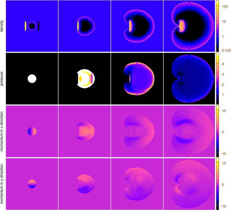
Figure 2: Simulation of a Sedov explosion on the domain $[0,1]\times[0,1]$. The variables are shown from top to bottom in the following order: density, pressure, velocity in the $x$- and velocity in the $y$-direction. From left to the right, snapshots in time are shown at $t=0.005$, $t=0.025$, $t=0.075$ and $t=0.15$. The initial condition is chosen as follows: the velocity is zero in both directions, the density is set to one except for a hill of 100 at the left and a basin of 0.01 at the right. The pressure is a sharp Gaussian distribution. The density forms a shock front which wraps around the density hill and is accelerated by the sink.

Figure 2 shows the behavior of the physical variables for a simple test problem on the domain $[0,1]\times[0,1]$. The snapshots are taken at time $t=0.005$, $t=0.025$, $t=0.075$, and $t=0.15$. As initial condition, we set a background density to $\rho=1$ with a density hill of $\rho=100$ on the left side and a density basin of $\rho=0.01$ on the right side of the domain. The pressure has a background value of $p=0.0001$ and a Gaussian with a peak of $1200$ and the standard deviation $\sigma=20.48$. Both the velocity in the $x$- and in the $y$-direction are $0$ at the beginning of the simulation.

Up to the time considered in the first column of Figure 2, the dynamics of the system is mainly determined by the variation in pressure (as the initial values for the other variables are constant). For the density field, a sharp front develops that spreads out symmetrically. This is the propagation of a shock front which we have discussed earlier. Note that the density variable varies over three orders of magnitude. Thus, we use a logarithmic scale in order to better observe the behavior of the solution. Such a scaling is not necessary for the other variables. The pressure flattens out very quickly during this time period where it causes an acceleration of the particles. To be able to observe the behavior of the pressure variable at the last shown time step, we limited the color range to a maximum of $5$ (the largest value is close to $49$; at time $t=0.005$).

In the second column, we see that the density shock wave hits the hill and the basin of the density field. For the hill, we observe that the shock wave is absorbed by the much higher density, while at the basin, it is drawn into the region of lower pressure. This behavior can be observed by the pressure variable as well. When we integrate further, the original shock wave wraps around the hill, until it completely envelopes the hill and vortices begin to form. The velocity variables show that the particles within the right part of the domain are further accelerated, while at the hill, there is almost no movement.

2.1 Structure of the sequential code

We start with a sequential code which we will parallelize both with MPI and UPC. The basic structure of the code is described in Algorithm 1.

⬇

set initial physical variables;

time loop

call_one_d in x-direction;

call_one_d in y-direction;

with the function

⬇

call_one_d:

change physical to conserved variables;

calculate the flux;

execute Godunov’s method;

change conserved to physical variables;

Algorithm 1 Pseudo code of the sequential implementation.

2.2 Parallelization: MPI

The MPI version of the code is based on the Single Program Multiple Data (SPMD) approach. The two-dimensional arrays for the four physical variables $\rho$, $u$, $v$ and $p$ are partitioned among the number of processes in a row-wise manner. In this simulation, we take a look at two different boundary conditions. In the $x$-direction, we use periodic boundary conditions, i.e., the left most grid point is identified with the right most grid point. In the $y$-direction, we consider an inflow condition at the bottom (i.e., the value at the bottom is a constant that we define as a global variable) and an outflow condition at the top (we just use the value on the top of the grid twice, which corresponds to Neumann boundary conditions). Since such a setting will lead to unintended reflections, we introduce a couple of ghost cells to hide these artifacts.

First, let us consider the partitioning of the domain in rows. This situation is illustrated in Figure 3. Due to the imposed boundary conditions, no MPI-communication is needed at the boundary of the domain. However, each process has to communicate with the two processes which are located immediately above and below of it (this is illustrated in Figure 3 and in more detail in Figure 4 for a simulation with four cores). Each process uses the non-blocking MPI_Isend and MPI_Irecv routines in order to transfer the necessary data. Note that no global synchronization is necessary.

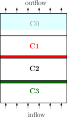
Figure 3: Setup for the core C2, where the physical variables are stored row-wise on the different cores. In the MPI implementation, the neighbors C1 in red and C3 in green prepare their bottom and top row respectively and send it via MPI_Isend to core C2. In the naive, pointer, and barrier UPC implementations, C2 accesses these rows directly via a shared array. In the UPC halo implementation, C2 fetches these rows via upc_memget without active involvement from the neighbors. Due to the outflow condition, additional ghost cells are necessary which are shown in cyan. Note that these cells can extend over more than a single thread. The setup is valid for the MPI row implementation as well as the naive, pointer, barrier, and halo UPC implementations.

Figure 4: Required communication diagram for the MPI row setup on four cores.

For comparison, we also consider the distribution of the data in patches. This framework exchanges less data but requires more MPI calls.

Since the data is no longer distributed row-wise on each core, both in the $x$- as well as in the $y$-direction, MPI-communication has to be performed using the non-blocking MPI routines. Similar to the row-wise decomposition, only communication with nearest neighbors is required.

In 5 we illustrate the partitioning of the data on sixteen cores and highlight the required communication for the core C5. In Figure 6, the communication pattern of this setup is demonstrated in a diagram for sixteen cores. For both implementations, the sequential code is extended with an additional function that communicates the boundary values (see Algorithm 2).

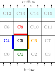
Figure 5: Setup for the core C5, where the physical variables are stored patch-wise on the different cores. In the MPI implementation, the neighbors C6 in orange, C9 in red, C4 in blue and C1 in green prepare their left, bottom, right and top row respectively and send it via MPI_Isend to core C5. In the UPC implementation, C5 fetches these rows via upc_memget without active involvement of the neighbors. Due to the outflow condition, additional ghost cells are necessary which are shown in cyan. Note that these cells can extend over more than a single thread. The setup is valid for the MPI patch implementation as well as the patch UPC implementation.

Figure 6: Required communication diagram for the MPI patch setup on sixteen cores.

⬇

set initial physical variables;

time loop

communicate boundaries in x-direction;

call_one_d in x-direction;

communicate boundaries in y-direction;

call_one_d in y-direction;

Algorithm 2 Pseudo code of the MPI implementation.

In each time step, first the boundaries in the $x$-direction are communicated and then the calculations in this direction are performed locally on each processor. To conclude the time step, the same is done in the $y$-direction.

2.3 Parallelization: UPC

For the UPC parallelization, we take advantage of the shared data structures provided by UPC. As discussed earlier, a big advantage of UPC is the incremental approach to parallelization. It is therefore possible to parallelize the sequential code by just adding a few additional lines to the sequential code. However, to obtain good scalability we require a more sophisticated implementation. We therefore introduce a sequence of optimization steps, whose performance we will analyze in the next section on different HPC systems.

For our first parallelization, which we call the naive approach, we just declare our work arrays as shared such that every processor can access it. Therefore, no visible communication is performed. However, the workload on each thread still has to be defined by the programmer. The cells with affinity to certain threads are distributed in rows similar to the MPI implementation that we discussed earlier (see Figure 3). Due to the assumed memory layout of UPC, this simplifies the implementation. Note that this data distribution is also valid for the next three implementations.

Since in the $x$-direction the slices are located on the same thread, all calculations can be done locally. However, in the $y$-direction, the cells are distributed among the threads. In this case, the communication is performed directly on the shared array which hides the communication (which is required to satisfy the remote access) from the user.

Our code has the form stated in Algorithm 3. In Figure 7, the communication of this setup is demonstrated in a diagram for four cores.

Figure 7: Required communication diagram for the UPC: row, pointer and barrier setups on four cores.

⬇

set shared initial physical variables;

time loop

call_one_d in x-direction:

do calculation;

call_one_d in y-direction:

use shared array for calculation;

Algorithm 3 Pseudo code of the naive UPC implementation.

In this implementation, communication is the bottleneck. Even though Thread 0 can access a data point on Thread 3, this might be very expensive, especially, if both processes do not reside on the same node. As a rule of thumb, shared variables are expensive to access, and thus accessing them one by one should be avoided, if possible. In our application, most of the memory access is local.

We call our second approach pointer approach, because in the $y$-direction, we create a pointer on each thread that only manipulates local data of the shared array slice, i.e. Algorithm 4.

⬇

set initial physical variables shared;

time loop

call_one_d in x-direction:

do calculation;

call_one_d in y-direction:

create local pointers to shared;

use local pointers for calc;

Algorithm 4 Pseudo code of the pointer UPC implementation.

In this implementation, the communication is still performed indirectly, by using the shared data array. The communication for sixteen cores is demonstrated in Figure 7 and the data distribution is still the same as above (see, e.g., Figure 3). In principle, this optimization can be performed by the UPC compiler. However, it is not clear, how efficient this optimization is in practice.

Similar to the OpenMP programming paradigm, we need to avoid race conditions, i.e., we need to make sure that when a calculation step takes information from a shared object the corresponding data point has already been updated. This is guaranteed by barriers. However, at barriers all threads have to wait for each other until they can continue with their work. This is accompanied with a significant overhead and thus, barriers should be used as little as possible in the code.

Using the performance tool upc_trace on our code we found that the barriers in our code are a significant bottleneck. Our next optimization step is therefore called the barrier approach, because we divided the calculation loop into two loops, so that we can move the barrier outside of the loop. The idea is demonstrated in Algorithm 5.

⬇

call_one_d in y direction:

define local calculation arrays glob;

start calculation loop

cast local pointers;

change physical to conserved variables in global array;

calculate the flux in global array;

end calculation loop;

barrier;

start calculation loop

cast local pointers;

execute Godunov’s method with global array;

change conserved to physical variables;

end calculation loop;

Algorithm 5 Pseudo code of the barrier UPC implementation.

In this case, we have to define some arrays that we need for the calculation globally (so that we can use them in the two loops). However, we only have to call the barrier once in each time step, removing a lot of overhead. Note that this approach only incurs a small overhead in the amount of memory used. The distribution and communication in this setup is the same as in the above method (see, e.g., Figure 3 and Figure 7).

Up to now, we only tried to exploit locality of the computation, but kept the main working array shared. As the next step, we used an idea which is usually implemented in MPI code: we do no longer work on the whole shared array, but use shared variables only for communicating ghost cells. Therefore, similar to MPI, the boundaries are communicated in a single call to upc_memget and the remainder of the computation is done locally. We thus name this level of optimization the halo approach (see Algorithm 6).

⬇

set initial physical variables shared;

get local copies of shared variables;

time loop

call_one_d in x-direction:

do calculation locally;

barrier;

get boundaries from shared array;

barrier;

call_one_d in y-direction:

do calculation locally;

Algorithm 6 Pseudo code of the halo UPC implementation.

In this implementation, the computation is completely local. The call upc_memget takes the necessary rows from the upper and lower neighbor without them actively participating in the communication. To avoid race conditions in this case, a synchronization barrier has to be included. The distribution of the data is still equivalent to the implementations above (see, e.g., Figure 3). In Figure 8, the communication of this setup is demonstrated for four cores.

Figure 8: Required communication diagram for the UPC: halo setup on four cores.

All the approaches above are distributed in a row-wise manner. However, this setup may lead to more communication than is necessary. A final optimization step is thus to distribute the data points on the threads in patches (see Figure 5). Since the data points are contiguous in the $x$-direction the data communication is done by a single call of upc_memget (as was done in the previous optimization step). To communicate the data in $y$-direction, we used the strided function upc_memget_strided. Note that this function is part of the Berkeley UPC compiler and not yet part of the UPC standard, however, it greatly facilitates the implementation. Again, to avoid race conditions, synchronization barriers have to be included. Due to the data distribution, we call this implementation the patch approach. Similar to the previous algorithm, this setup performs only local computation. The communication for sixteen cores is demonstrated in Figure 9.

Figure 9: Required communication diagram for the UPC: patch setup on sixteen cores.

An overview for the different types of distribution, communication and computation is given in Table 1.

		distribution	computation	comm: $x$-direction	comm: $y$-direction
				left & right boundary	top & bottom boundary
MPI	row	row-wise	local	none	Isend/Irecv
	patch	patch-wise	local	Isend/Irecv	Isend/Irecv
UPC	naive	row-wise	on shared array	none	implicit
	pointer	row-wise	local, on shared array	none	implicit
	barrier	row-wise	local, on shared array	none	implicit
	halo	row-wise	local	none	upc_memget
	patch	patch-wise	local	upc_memget	upc_memget

Table 1: Overview between different MPI and UPC implementations.

As we can see, the optimization steps are getting more and more sophisticated and the code gets more and more involved. However, changing and debugging the code incrementally is usually much easier than writing an already perfectly optimized version in the first place. The scaling behavior of the different approaches on different hardware is discussed in the next section.

3 Results

In this section we investigate the scaling behavior of the different codes described in the previous section and compare the results on different hardware. For this purpose, we have access to four different HPC systems. LEO3 and LEO3E are local clusters at the University of Innsbruck. Assembled in 2011 with 162 compute nodes, LEO3 is a medium sized but relatively old cluster. In 2015, the computing infrastructure in Innsbruck was extended by a smaller but more modern system, LEO3E, with 45 computing nodes. Both systems have approximately equal peak performance.

In addition, we also use the main high performance facility in Austria: the Vienna Scientific Cluster (VSC). In this study, we use VSC2, which ranked 56 of the Top 500 systems when it came into operation in 2011 and consists of 1314 computing nodes. In addition, we consider VSC3, which occupied rank 85 of the Top 500 systems in its first year of operation (2014) and consists of 2020 computing nodes.

We therefore have the opportunity to compare Tier 2 with Tier 1 systems as well as relatively old with relatively new hardware.

All of the above systems are relatively traditional high performance cluster models. We believe that such systems are representative for the HPC resources available to most researchers.

Since the shared memory model used by UPC is a natural fit for the Intel Xeon Phi, we also investigate the scaling behavior of our implementation on that platform. The Xeon Phi implements a many-core architecture (similar to graphic processing units) with 60 physical cores (240 cores are available for hyperthreading). Since the cores of the Xeon Phi are based on an x86 architecture, it is relatively straightforward to compile a UPC program for it.

For detailed hardware specifications, see Table 2.

system	nodes	CPU on node	cores	memory	Rpeak	nw controller
LEO3	162	2 x Intel Xeon X5650, 2.7 GHz	12	4 TB	18 TFlop/s	Mellanox
LEO3E	45	2 x Intel Xeon E5-2650-v3, 2.6 GHz	10	4 TB	29 TFlop/s	Mellanox
VSC2	1314	2 x AMD Opteron 6132HE, 2.2GHz	8	42 TB	185 TFlop/s	Mellanox
VSC3	2020	2 x Intel Xeon E5-2650v2, 2.6GHz	8	131 TB	682 TFlop/s	Intel

Table 2: Hardware specifications for the four clusters used in this paper.

On each system, we execute both a strong as well as a weak scaling analysis. For the strong scaling analysis, we choose a fixed problem size and run the program on different number of cores. Ideally, the run time would decrease linearly in the number of cores. In this paper, we choose our problem size as a grid of $512\times 1024$ points and a final time $T=0.005$.

The weak scaling analysis is performed by increasing the grid according to the number of cores. Ideally, the time it takes to finish the larger problem would remain constant. In our case, we choose for one core a domain with $64\times 128$ grid points and a final integration time of $T=0.001$. When quadrupling the number of cores, we quadruple the problem size by choosing a grid of $128\times 256$ for four cores, etc.

In our simulations we use a constant time step size $\Delta t=10^{-5}$ (which is small enough such that the CFL condition is always satisfied).

3.1 Results on LEO3

On LEO3 we use up to 256 cores. Even though the network adapter is from Mellanox and thus in theory would support the network option mxm (which uses the InfiniBand library provided by Mellanox) for UPC, the driver version present on the system is too old to work with UPC. We therefore use ibv (InfiniBand verbs which is a generic library used to access the InfiniBand hardware) as the network type. The results are shown in Figure 10 and Table 3.

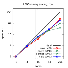
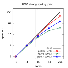
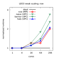
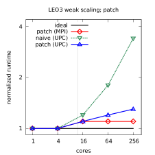
Figure 10: This figure shows the scaling results on the LEO3. The left hand side shows from top to bottom the strong and the weak scaling results for the row-wise communication pattern. Due to the similar results of the UPC row and pointer version, we only include the first one in the plot. The right hand side shows from top to bottom the strong and the weak scaling results for the patched communication pattern. For comparison, this column also includes the row-wise distributed naive UPC version. The black line represents the ideal scaling in all cases. The gray line represents the number of cores where the simulation can be run on a single node. For the LEO3, this line is at 12 cores.

LEO3, strong scaling
	MPI				UPC
threads	row		patch		naive		pointer		barrier		halo		patch
1	982.	8 00(1.0)	977.	9 00(1.0)	921.	4 0(1.0)	897.	0 0(1.0)	903.	0 0(1.0)	930.	0 0(1.0)	943.	2 0(1.0)
4	287.	9 00(3.4)	249.	1 00(3.9)	253.	8 0(3.6)	242.	6 0(3.7)	243.	5 0(3.7)	253.	7 0(3.7)	234.	9 0(4.0)
16	107.	8 00(9.1)	63.	7 0(15.4)	83.	7 (11.0)	81.	1 (11.1)	79.	6 (11.3)	76.	7 (12.1)	72.	9 (12.9)
64	35.	4 0(27.8)	17.	5 0(55.9)	36.	1 (25.5)	34.	8 (25.8)	31.	6 (28.6)	30.	3 (30.7)	27.	0 (34.9)
256	9.	2 (106.8)	6.	4 (152.8)	25.	7 (35.9)	18.	1 (49.6)	14.	6 (61.8)	10.	2 (91.2)	11.	7 (80.6)

LEO3, weak scaling
		MPI				UPC
threads	grid	row		patch		naive		pointer		barrier		halo		patch
1	$64\times\phantom{0}128$	3.	0 (1.0)	3.	0 (1.0)	2.	8 (1.0)	2.	6 (1.0)	2.	6 (1.0)	2.	5 (1.0)	2.	6 (1.0)
4	$128\times\phantom{0}256$	3.	1 (1.0)	3.	1 (1.0)	3.	0 (1.0)	2.	6 (1.1)	2.	6 (1.0)	2.	6 (1.0)	2.	6 (1.0)
16	$256\times\phantom{0}512$	3.	6 (1.2)	3.	2 (1.1)	3.	4 (1.2)	3.	6 (1.4)	2.	9 (1.1)	2.	7 (1.1)	2.	9 (1.1)
64	$512\times 1024$	4.	8 (1.6)	3.	2 (1.1)	4.	9 (1.8)	4.	6 (1.8)	3.	7 (1.4)	3.	3 (1.3)	3.	2 (1.2)
256	$1024\times 2048$	6.	0 (2.0)	3.	4 (1.1)	9.	5 (3.4)	9.	5 (3.6)	6.	7 (2.6)	5.	4 (2.1)	3.	5 (1.3)

Table 3: This table shows the strong and weak scaling results on the LEO3 system. For the strong scaling analysis, we used the grid $512\times 1024$. In addition to the runtime, we also include the speedup (for the strong scaling analysis) and the increase in runtime normalized to the single core implementation (for the weak scaling). These quantities are shown in parenthesis.

row-wise communication pattern: On a single node, the strong scaling analysis for all of the UPC implementations exceed the results of the MPI version. However, as soon as we leave the node, the speedup dramatically depends on the optimization level of the implementation. The halo implementation competes with the speedup of the MPI program. Similar results are observed for the weak scaling analysis.

patched communication pattern: For this communication pattern, the single node performance is similar for strong as well as weak scaling for the MPI and the UPC version. However, the overhead for the UPC version seems to be higher as soon as we run the simulation on a larger number of nodes.

3.2 Results on LEO3E

Similar to LEO3, we can not take advantage of the Mellanox network driver for the UPC code. Therefore, ibv is used as the network type. The results for LEO3E can be found in Figure 11 and Table 4.

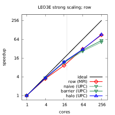
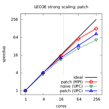
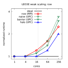
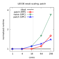
Figure 11: This figure shows the scaling results on the LEO3E. The left hand side shows from top to bottom the strong and the weak scaling results for the row-wise communication pattern. Due to the similar results of the UPC row and pointer version, we only include the first one in the plot. The right hand side shows from top to bottom the strong and the weak scaling results for the patched communication pattern. For comparison, this column also includes the row-wise distributed naive UPC version. The black line represents the ideal scaling in all cases. The gray line represents the number of cores where the simulation can be run on a single node. For the LEO3E, this line is at 20 cores.

LEO3E, strong scaling
	MPI				UPC
threads	row		patch		naive		pointer		barrier		halo		patch
1	849.	4 0(1.0)	843.	9 00(1.0)	616.	7 0(1.0)	580.	9 0(1.0)	599.	7 0(1.0)	595.	8 0(1.0)	610.	8 0(1.0)
4	242.	7 0(3.5)	212.	5 00(4.0)	169.	7 0(3.6)	156.	9 0(3.7)	161.	0 0(3.7)	159.	4 0(3.7)	148.	7 0(4.1)
16	91.	4 0(9.3)	56.	5 0(14.9)	54.	3 (11.4)	50.	8 (11.4)	50.	3 (11.9)	49.	4 (12.1)	47.	9 (12.8)
64	27.	4 (31.0)	14.	9 0(56.6)	23.	2 (26.6)	23.	4 (24.8)	20.	8 (28.8)	19.	4 (30.7)	18.	2 (33.6)
256	9.	6 (88.5)	6.	7 (126.0)	11.	8 (52.3)	11.	2 (51.9)	10.	2 (58.8)	6.	5 (91.7)	7.	3 (83.7)

LEO3E, weak scaling
		MPI				UPC
threads	grid	row		patch		naive		pointer		barrier		halo		patch
1	$64\times\phantom{0}128$	2.	6 (1.0)	2.	5 (1.0)	1.	8 (1.0)	1.	7 (1.0)	1.	7 (1.0)	1.	7 (1.0)	1.	7 (1.0)
4	$128\times\phantom{0}256$	2.	6 (1.0)	2.	6 (1.0)	1.	8 (1.0)	1.	7 (1.0)	1.	7 (1.0)	1.	7 (1.0)	1.	7 (1.0)
16	$256\times\phantom{0}512$	3.	0 (1.2)	2.	6 (1.0)	2.	0 (1.1)	1.	9 (1.1)	1.	9 (1.1)	1.	7 (1.0)	1.	9 (1.1)
64	$512\times 1024$	4.	1 (1.6)	2.	7 (1.1)	2.	9 (1.6)	2.	8 (1.6)	2.	4 (1.4)	2.	0 (1.2)	2.	1 (1.2)
256	$1024\times 2048$	6.	5 (2.5)	4.	1 (1.6)	6.	2 (3.4)	6.	0 (3.5)	5.	1 (3.0)	3.	4 (2.0)	2.	4 (1.4)

Table 4: This table shows the strong and weak scaling results on the LEO3E system. For the strong scaling analysis, we used the grid $512\times 1024$. In addition to the runtime, we also include the speedup (for the strong scaling analysis) and the increase in runtime normalized to the single core implementation (for the weak scaling). These quantities are shown in parenthesis.

The processors on this hardware are newer and thus faster than on LEO3. This can be seen in the significantly shorter runtime of the sequential code (see, e.g., Table 4).

row-wise communication pattern: On a single node, the different optimization stages of the UPC code are similar and compete with the MPI version. For a larger number of nodes, the halo version scales better compared to the MPI program. This is valid for both the strong as well as the weak scaling analysis.

patched communication pattern: The speedup for the strong scaling analysis of the MPI version is better than the UPC program. However, for the weak scaling analysis, UPC scales better compared to the MPI version.

3.3 Results on VSC2

VSC2 uses a Mellanox adapter and we are able to make use of the mxm-network type. For this system, we experience a significant performance issue brought about by the synchronization barriers in our code. Due to the significant run time increase for the naive, pointer, and barrier UPC runs, we only compare the halo implementation with MPI (Figure 12 and Table 5). Since the VSC2 system is larger than LEO3 and LEO3E, we perform a weak scaling analysis for up to 1024 cores. This can not be done for strong scaling, since due to the data distribution of the UPC code, we have not enough data points for the problem size considered.

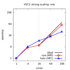
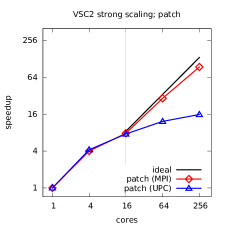
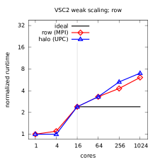
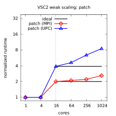
Figure 12: This figure shows the scaling results on the VSC2. The left hand side shows from top to bottom the strong and the weak scaling results for the row-wise communication pattern. Due to the significant run time increase for the naive, pointer, and barrier UPC runs, we only compare the halo implementation. The right hand side shows from top to bottom the strong and the weak scaling results for the patched communication pattern. Since the architecture of the AMD CPU only includes a single floating point unit for every two cores, perfect scaling on one node is not expected and not achieved. In that respect, we only included the ideal scaling line in black when the simulation leaves one node. The gray line represents the number of cores where the simulation can be run on a single node. For the VSC2, this line is at 16 cores.

VSC2, strong scaling
	MPI				UPC
threads	row		patch		halo		patch
1	1615.	6 0(1.0*)	1535.	7 0(1.0*)	1649.	9 (1.0*)	1653.	2 (1.0*)
4	451.	4 0(3.6*)	380.	6 0(4.0*)	415.	2 (4.0*)	391.	9 (4.2*)
16	337.	2 0(4.8*)	196.	6 0(7.8*)	197.	5 (8.4*)	217.	0 (7.6*)
64	102.	4 0(3.3*)	52.	9 0(3.8*)	119.	9 (1.6*)	135.	6 (1.6*)
256	28.	6 (11.8*)	16.	3 (12.1*)	65.	4 (3.0*)	104.	9 (2.1*)

VSC2, weak scaling
		MPI				UPC
threads	grid	row		patch		halo		patch
1	$64\times\phantom{0}128$	4.	5 (1.0*)	4.	5 (1.0*)	4.	4 (1.0*)	4.	4 (1.0*)
4	$128\times\phantom{0}256$	4.	8 (1.1*)	4.	6 (1.0*)	4.	3 (1.0*)	4.	2 (1.0*)
16	$256\times\phantom{0}512$	11.	0 (2.4*)	9.	2 (2.0*)	10.	5 (2.4*)	17.	0 (3.9*)
64	$512\times 1024$	14.	9 (1.4*)	9.	6 (1.0*)	14.	9 (1.4*)	20.	1 (1.2*)
256	$1024\times 2048$	19.	3 (1.8*)	9.	8 (1.1*)	23.	2 (2.2*)	28.	1 (1.7*)
1024	$2048\times 4096$	27.	5 (2.5*)	11.	6 (1.3*)	30.	9 (2.9*)	37.	3 (2.2*)

Table 5: This table shows the strong and weak scaling results on the VSC2 system. For the strong scaling analysis, we used the grid $512\times 1024$. In addition to the runtime, we also include the speedup (for the strong scaling analysis) and the increase in runtime normalized to the single core implementation (for the weak scaling). These quantities are shown in parenthesis. The numbers denoted with * are not based on one core but on 16 cores due to the hardware properties described in the text.

Due to the architecture of the AMD CPU, which includes only a single floating point unit for every two cores, we only observe a speedup of 8 on a single node. This is an inherent limitation of the CPU and can be observed for both the MPI as well as the UPC implementation.

row-wise communication pattern: We observe that the single node performance of the UPC halo implementation outperforms the MPI version. However, as soon as we use a higher number of nodes, the performance is disappointing for UPC. This is a result of the fact that a large portion of the run time is spend in the two calls (per time step) to upc_barrier (see Table 5).

patched communication pattern: Similar to the row pattern implementations, the single node performance of the MPI and the UPC implementation is comparable, however, the more cores are used, the more time is spend at the upc_barrier calls that significantly increases the run time of UPC. However, it should be noted that the scaling behavior of the MPI code is also far from ideal on this system.

3.4 Results on VSC3

VSC3 has an InfiniBand network adapter from Intel. Since Berkeley UPC does not include native support for this hardware, we use ibv as the network type. VSC3 is the largest system we have at our disposal. We therefore perform the weak scaling analysis for up to 1024 cores.

However, for problems with 1024 or more cores, by default, the UPC run time opens more InfiniBand connections than the hardware supports. In principle, to address this issue, XRC and SRQ were developed. Unfortunately, these technologies are not supported on VSC3. Thus, we have to bundle the network connections manually by reducing the number of processes on a single node. In UPC, this is accomplished by setting the pthread option on the command line. Increasing the number of pthreads also leads to an increase of the run time. We therefore only use the smallest number of pthreads possible. I.e., for $1024$ threads, we use $pthreads=2$. The detailed results can be found in Table 6 and a visual representation of the data is shown in Figure 13.

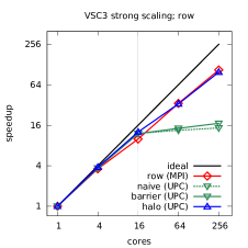
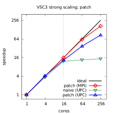
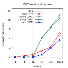
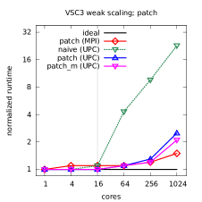
Figure 13: This figure shows the scaling results on the VSC3. The left hand side shows from top to bottom the strong and the weak scaling results for the row-wise communication pattern. Due to the similar results of the UPC row and pointer version, we only include the first one in the plot. The right hand side shows from top to bottom the strong and the weak scaling results for the patched communication pattern. For comparison, this column also includes the row-wise distributed naive UPC version and an additional modified UPC patch version patch_m (patch_mod in Table 6). In this version, more data is communicated in less communication steps. The black line represents the ideal scaling in all cases. The gray line represents the number of cores where the simulation can be run on a single node. For the VSC3, this line is at 16 cores.

VSC3, strong scaling, MPI
threads	row		patch
1	532.	2 00(1.0)	535.	8 00(1.0)
4	149.	5 00(3.6)	132.	9 00(4.0)
16	53.	2 0(10.0)	33.	7 0(15.9)
64	15.	7 0(33.9)	8.	7 0(61.6)
256	5.	0 (106.4)	3.	2 (167.4)

VSC3, weak scaling, MPI
threads	grid	row		patch
1	$64\times\phantom{0}128$	1.	5 (1.0)	1.	5 (1.0)
4	$128\times\phantom{0}256$	1.	6 (1.1)	1.	6 (1.1)
16	$256\times\phantom{0}512$	1.	8 (1.2)	1.	6 (1.1)
64	$512\times 1024$	2.	4 (1.6)	1.	6 (1.1)
256	$1024\times 2048$	3.	2 (2.1)	1.	8 (1.2)
1024	$2048\times 4096$	8.	8 (5.7)	2.	3 (1.5)

VSC3, strong scaling, UPC
threads	naive		pointer		barrier		halo		patch		patch_mod
1	516.	5 0(1.0)	459.	1 0(1.0)	478.	1 0(1.0)	482.	2 0(1.0)	478.	3 0(1.0)	478.	0 0(1.0)
4	141.	2 0(3.7)	123.	8 0(3.7)	128.	2 0(3.7)	125.	9 0(3.8)	116.	8 0(4.1)	117.	9 0(4.1)
16	42.	6 (12.1)	37.	8 (12.1)	39.	8 (12.0)	38.	0 (12.7)	36.	3 (13.2)	36.	1 (13.2)
64	38.	3 (13.5)	37.	0 (12.4)	33.	3 (14.4)	14.	5 (33.3)	12.	8 (37.4)	12.	7 (37.6)
256	35.	3 (14.6)	34.	2 (13.4)	28.	0 (17.1)	4.	9 (98.4)	5.	6 (85.4)	5.	5 (86.9)

VSC3, weak scaling, UPC
threads	naive		pointer		barrier		halo		patch		patch_mod
1	1.	5 00(1.0)	1.	3 00(1.0)	1.	3 00(1.0)	1.	3* (1.0)	1.	3* (1.0)	1.	3* (1.0)
4	1.	5 00(1.0)	1.	3 00(1.0)	1.	3 00(1.0)	1.	3* (1.0)	1.	3* (1.0)	1.	3* (1.0)
16	1.	6 00(1.1)	1.	4 00(1.1)	1.	3 00(1.0)	1.	3* (1.0)	1.	3* (1.0)	1.	3* (1.0)
64	6.	4 00(4.3)	6.	1 00(4.7)	5.	6 00(4.2)	1.	6* (1.2)	1.	4* (1.1)	1.	4* (1.1)
256	14.	3 00(9.6)	14.	6 0(11.2)	11.	8 00(8.9)	2.	6* (2.0)	1.	7* (1.3)	1.	6* (1.2)
1024	34.	2* (22.8)	33.	8* (26.0)	23.	7* (18.2)	4.	5* (3.5)	3.	3* (2.5)	2.	7* (2.1)

Table 6: This table shows the strong and weak scaling results on the VSC3 system. For the strong scaling analysis, we used the grid $512\times 1024$. In addition to the runtime, we also include the speedup (for the strong scaling analysis) and the increase in runtime normalized to the single core implementation (for the weak scaling). These quantities are shown in parenthesis. The numbers marked with a * are simulated by using 2 pthreads. This issue is discussed further within the text.

In this simulation, we have the newest as well as largest cluster within this paper at our disposal. This already affects the run time for one core, which is nearly half of the run time on the LEO3 system for all of the runs investigated.

row-wise communication pattern: Similar to the other hardware, all UPC optimization stages perform similarly on the same node. However, for a larger number of nodes, only the UPC halo version is able to compete with the MPI implementation. The strong scaling analysis is comparable for both implementations. For $1024$ cores, the weak scaling results for the halo UPC implementation significantly outperforms the MPI implementation.

patched communication pattern: The MPI version shows better scaling results than the UPC version. Since on this hardware, a significant amount of time is spend in the barriers, we also include the results for a modified patch version patch_mod: In this version, we communicate the data both in the $x$- as well as the $y$-direction before the splitting. This means that in each time step, we only communicate once, but twice as many data. This enables us to get rid of two barriers that are necessary to avoid race conditions in the patch implementation. Note that this is a first order approximation, even though the boundary data in the $y$-direction is not updated with the output from the splitting step in the $x$-direction, but from the data of the previous time step.

As we can see, the runtime for both patched versions only differs, when we reach a large number of nodes. On LEO3, LEO3E and VSC2 we observed no performance difference for these two versions. For this reason, we only include this additional optimization for VSC3. We can see that especially for more than a thousand cores, the overhead of the barriers have a significant impact. However, for this communication pattern, UPC can still not compete with MPI on the VSC3.

3.5 Results on the Intel Xeon Phi

Note that the Intel Xeon Phi usually benefits from additional vectorization optimizations. However, in this paper we use our most optimized UPC run as well as our MPI run without any change. The Intel Xeon Phi has 60 cores and 4 hyperthreads at each core that we could use. Note, however, that even with hyperthreading, we do not expect a linear increase after 60 cores. We only use the row implementation for MPI and the UPC halo version in this section. In Figure 14 and Table 7, we show the results for strong scaling for both CPUs on a single node and for the Intel Xeon Phi.

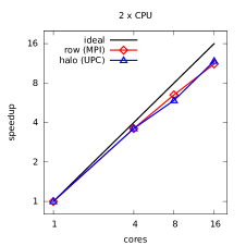
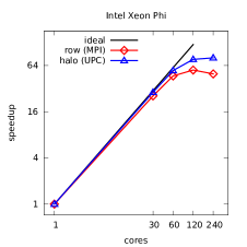
Figure 14: This figure shows the strong scaling results for the Intel Xeon Phi. The left hand side shows the scaling behavior of the two CPUs (Intel Xeon E5-2630 v3) present in that system. The right hand side shows the scaling on the Intel Xeon Phi 7120 for up to 240 threads. The black line represents the ideal scaling in both cases.

2$\times$CPU
threads	MPI: row		UPC: halo
1	3.	58 0(1.0)	3.	08 0(1.0)
4	0.	99 0(3.6)	0.	86 0(3.6)
8	0.	55 0(6.5)	0.	52 0(5.9)
16	0.	32 (11.2)	0.	26 (11.8)

       Intel Xeon Phi threads MPI: row UPC: halo 1 45. 83 0(1.0) 33. 06 0(1.0) 30 1. 78 (25.7) 1. 15 (28.7) 60 0. 98 (46.8) 0. 60 (55.1) 120 0. 82 (55.9) 0. 43 (76.9) 240 0. 92 (49.8) 0. 41 (80.6)

Table 7: This table shows the strong scaling results with the grid $512\times 1024$ on the Intel Xeon Phi system. The left analysis is performed on the two E5-2630v3 CPUs within that system. The left analysis is performed on the Intel Xeon Phi 7120. We also include the speedup in parenthesis. The grid size in $y$-direction is a multiple of $60$. The final integration time is $T=5\cdot 10^{-5}$.

Since UPC exploits the shared memory architecture (comparable to OpenMP), we see that it is a good fit for the Intel Xeon Phi. The scaling results for the UPC implementation are better by a factor of $1.6$ compared to the MPI implementation. We therefore conclude that UPC is a viable option for programming accelerators.

3.6 Productivity

Regarding the productivity of developing code with UPC as opposed to MPI, there two considerations. First, how much effort is required to obtain a working parallelization which at least scales to a couple of nodes. Second, how difficult is it to improve such a program to match or even exceed the performance of MPI. In the following we will discuss these two points.

Regarding the increasing difficulty of the more performant implementations in UPC, we identify the three versions naive, pointer and barrier as significantly more productive with respect to code development. The development effort of these parallelizations is comparable to OpenMP (and thus is significantly less involved than writing an MPI program).

If the developer is interested in strong scaling, the barrier version already achieves a speedup of $28.8$/$26.6$ on 64 cores and $58.8$/$52.3$ on 256 cores on a modern system (LEO3E/LEO3). This already exceeds the theoretical performance of OpenMP, since this is limited by the number of cores on a node (in this case 20/12). Compared with MPI, these speedups may be a significant margin away from the ideal speedup of $64$ and $256$ respectively (which can be achieved with an optimized MPI or UPC version).

In the case of weak scaling, we can, for example, run the barrier version on 64 and 256 cores on the LEO3E/LEO3. For 64 cores, the runtime increases by a factor of $1.4$/$1.4$ and for 256 cores, it increases by a factor of $2.5$/$3.0$ compared to the serial implementation. This means that on 64 cores we can solve, in the same amount of time, a problem which is $2.3$/$3.8$ times as large as an ideal OpenMP implementation would admit (which can use at most 20/12 cores). For 256 cores we can solve a problem which is $4.3$/$8.5$ times as large as an ideal OpenMP implementation is able to handle in the same time.

Therefore, we conclude that on modern hardware we can obtain a significant speedup compared to any implementation that only operates on a single node, while the development effort is comparable to OpenMP (significantly less of what would be required to do an MPI implementation). In addition, UPC enables us to further optimize our code in order to obtain performance that is comparable to MPI (this is done for the halo and patch implementations). Of course, this requires additional development effort. In that respect, a major advantage concerning productivity, in our opinion, is the incremental approach for parallelism in UPC. The possibility of debugging only small changes leads to a significant reduction in development time for the different versions of the program.

4 Conclusion

In this paper, we investigate the usability of the PGAS language UPC for a scientific code and its competitiveness with MPI. We use a basic fluid dynamics code to solve the Euler equations of gas dynamics and parallelized it with both MPI and different optimization stages of UPC for two different communication patterns. Then, we compare the results on different hardware systems by conducting a strong and a weak scaling analysis, respectively.

We find that in most cases, for the row implementation UPC exceeds the MPI implementation. However, for the patched implementation, MPI scales usually better.

We experience a major drawback at VSC2, where barriers prove to be extremely expensive. This issue is not nearly as significant for the other hardware. Furthermore, on more than 1024 cores on VSC3 the efficiency of connection bundling degrades the performance.

Despite these issues, especially the possibility of incremental parallelization convinces us that UPC is a viable option for scientific computing on these HPC systems.

5 Acknowledgments

We want to thank Paul Hargrove (Lawrence Berkeley National Laboratory) for helping us to set up UPC on VSC3. We also want to thank Martin Thaler (ZID, University of Innsbruck) for helping us to set up UPC on LEO3 and LEO3E.

This paper is based upon work supported by the VSC Research Center funded by the Austrian Federal Ministry of Science, Research and Economy (bmwfw). The computational results presented have been achieved in part using the Vienna Scientific Cluster (VSC). This work was supported by the Austrian Ministry of Science BMWF as part of the UniInfrastrukturprogramm of the Focal Point Scientific Computing at the University of Innsbruck.

References

- [1] The Berkeley UPC Compiler. http://upc.lbl.gov/, 2015.
- [2] F. Cantonnet, Y. Yao, M. Zahran, and T. El-Ghazawi. Productivity analysis of the UPC language. In Parallel and Distributed Processing Symposium, 2004. Proceedings. 18th International. IEEE, 2004.
- [3] S. Chauvin, P. Saha, F. Cantonnet, S. Annareddy, and T. El-Ghazawi. UPC manual. The George Washington University High Performance Computing Laboratory, 2003.
- [4] UPC Consortium et al. UPC language specifications v1.3. Lawrence Berkeley National Laboratory, 2013.
- [5] N. Jansson and J. Hoffman. Improving Parallel Performance of FEniCS Finite Element Computations by Hybrid MPI/PGAS. preprint, http://www.diva-portal.org/smash/record.jsf?pid=diva2%3A618543&dswid=-9130, 2015.
- [6] H. Jin, R. Hood, and P. Mehrotra. A practical study of UPC using the NAS parallel benchmarks. In Proceedings of the Third Conference on Partitioned Global Address Space Programing Models. ACM, 2009.
- [7] J. Jose, K. Hamidouche, X. Lu, S. Potluri, J. Zhang, K. Tomko, and D. Panda. High performance OpenSHMEM for Xeon Phi clusters: Extensions, runtime designs and application co-design. In 2014 IEEE International Conference on Cluster Computing (CLUSTER). IEEE, 2014.
- [8] A. Kamil. Analysis of Partitioned Global Address Space Programs. PhD thesis, Department of Electrical Engineering and Computer Sciences, University of California at Berkeley, 2006.
- [9] R. LeVeque. Numerical methods for conservation laws. Springer, 1992.
- [10] R. LeVeque. Finite volume methods for hyperbolic problems. Cambridge university press, 2002.
- [11] M. Luo, M. Li, A. Venkatesh, X. Lu, and D. Panda. UPC on MIC: early experiences with native and symmetric modes. In Proceedings of the 7th International Conference on PGAS Programming Models, 2013.
- [12] A. Mallinson, D. Beckingsale, W. Gaudin, J. Herdman, J Levesque, and S. Jarvis. Cloverleaf: Preparing hydrodynamics codes for exascale. In A New Vintage of Computing : CUG2013, Napa, CA.
- [13] A. Mallinson, S. Jarvis, W. Gaudin, and J. Herdman. Experiences at scale with PGAS versions of a hydrodynamics application. In Proceedings of the 8th International Conference on Partitioned Global Address Space Programming Models. ACM, 2014.
- [14] D. Mallón, G. Taboada, C. Teijeiro, J. Touriño, B. Fraguela, A. Gómez, R. Doallo, and J. Mouriño. Performance evaluation of MPI, UPC and OpenMP on multicore architectures. In Recent Advances in Parallel Virtual Machine and Message Passing Interface. Springer, 2009.
- [15] H. Shan, H. Jin, K. Fuerlinger, A. Koniges, and N. Wright. Analyzing the effect of different programming models upon performance and memory usage on cray XT5 platforms. In Cray User’s Group Meeting 2010. Edinburgh, May 2010., 2010.
- [16] C. Simmendinger, J. Jägersküpper, R. Machado, and C. Lojewski. A PGAS-based implementation for the unstructured CFD solver TAU. In Proceedings of the 5th Conference on Partitioned Global Address Space Programming Models, PGAS, 2011.
- [17] E. Toro. Riemann solvers and numerical methods for fluid dynamics: a practical introduction. Springer, 2009.
- [18] K. Yelick, D. Bonachea, W. Chen, P. Colella, K. Datta, J. Duell, S. Graham, P. Hargrove, P. Hilfinger, P. Husbands, C. Iancu, A. Kamill, R. Nishtala, J. Su, M. Welcome, and T. Wen. Productivity and performance using partitioned global address space languages. In Proceedings of the 2007 international workshop on parallel symbolic computation, New York. ACM, 2007.
- [19] Z. Zhang and S. Seidel. Benchmark measurements of current UPC platforms. In 19th IEEE International Parallel and Distributed Processing Symposium. IEEE, 2005.