Strong-field effects in the photo-emission spectrum of the $\text{C}_{60}$ fullerene

Abstract

Considering $\text{C}_{60}$ as a model system for describing field emission from the extremity of a carbon nanotip, we explore electron emission from this fullerene excited by an intense, near-infrared, few-cycle laser pulse ($10^{13}$-$10^{14}\leavevmode\nobreak\ \text{W}/\text{cm}^{2}$, 912 nm, 8-cycle). To this end, we use time-dependent density functional theory augmented by a self-interaction correction. The ionic background of $\text{C}_{60}$ is described by a soft jellium model. Particular attention is paid to the high energy electrons. Comparing the spectra at different emission angles, we find that, as a major result of this study, the photoelectrons are strongly peaked along the laser polarization axis forming a highly collimated electron beam in the forward direction, especially for the high energy electrons. Moreover, the high-energy plateau cut-off found in the simulations agrees well with estimates from the classical three-step model. We also investigate the build-up of the high-energy part of a photoelectron spectrum by a time-resolved analysis. In particular, the modulation on the plateau can be interpreted as contributions from intracycle and intercycle interferences.

I Introduction

Emission from nanometric tips subject to possibly intense laser fields is of strong current interest as it constitutes a promising source of a well collimated and coherent beam of ultrafast electrons Hilbert et al. (2009), which can be used in electron diffraction experiments Williamson et al. (1997) as well as electron microscopy Lobastov et al. (2005). Such systems could be especially interesting in the recollision regime (in which emitted electrons recollide with the tip in the course of the laser pulse) as this could allow to generate extremely short electron pulses Paul et al. (2001) and thus pave the way to sub-femtosecond and sub-nanometric probing of matter Agostini and DiMauro (2004). Most studies have up to now focused on metallic nanotips. In particular, laser-induced photo-emission of electrons in the recollision regime, manifesting itself in the formation of a plateau at high kinetic energies in the photo-electron spectrum (PES), has been very recently observed in tungsten tips of nanometric size Bormann et al. (2010); Schenk et al. (2010); Krüger et al. (2012a). In this context, carbon nanotubes have also been proposed as promising emitting devices, since they possess an even smaller tip size than the metal tips used so far Carroll et al. (1997). These novel structures have mainly been characterized by field emission experiments Saito et al. (1997); Nilius et al. (2000). Due to this smaller tip size of carbon nanotubes, these systems might thus lead to even more promising sources for sub-femtosecond / sub-nanometric probing of dynamic processes in various areas of physics, chemistry, biochemistry or material science. Only very recently, laser-assisted photo-electron studies, which have been very successful in the case of metal nanotips, have been extended to these novel tips based on carbon nanostructures Bionta et al. (2014).

In relation to this question of field emission from carbon nanotips, the present work aims at studying to which extent photo-emission by ultrafast laser pulses can reach the intended recollision regime in carbon nanostructures. As a starting point, we shall focus our analysis on the actual extremity of the tip which practically consists in the cap of a nanotube (the tip is formed by rolling graphene sheets with various radii and helical structures). The cap of the carbon nanotubes used in the above mentioned photo-emission experiments are similar in size and structure to a $\text{C}_{60}$ cluster Saito et al. (1992). In this first step we shall thus use $\text{C}_{60}$ as a test model for the exploratory studies presented here. We consider the response of $\text{C}_{60}$ subject to an intense laser irradiation and characterize this response in terms of photo-electron spectra (PES).

The paper is outlined as follows: Section II briefly introduces the theoretical framework and computational details. Section III presents and discusses the results. Section IV completes the paper with a conclusion.

II Formal framework

II.1 Time-dependent local-density approximation

We describe electron dynamics by means of time-dependent density-functional theory at the level of the time-dependent local-density approximation (TDLDA). The LDA is complemented by an average-density self-interaction correction (SIC), which has been shown to provide a reliable theoretical framework of electron dynamics in strong laser fields, in particular when the excitation leads to substantial ionization  Kawashita et al. (2009); Fennel et al. (2010). The detailed theoretical approach is given elsewhere, and shall only briefly be summarized here. The time-dependent single-particle (s.p.) wave functions $\varphi_{j}(\textbf{r},t)$ are obtained by solving the time-dependent Kohn-Sham equations Runge and Gross (1984) (here and in the following we use atomic units) :

$$\mathrm{i}\frac{\partial}{\partial t}\varphi_{j}(\textbf{r},t) = \{-\frac{1}{2}\nabla^{2}+\upsilon_{\mathrm{C}}[\rho(\textbf{r},t)]$$ (1b)

$$\quad+\ \upsilon_{\mathrm{xc}}[\rho(\textbf{r},t)]+\upsilon_{\mathrm{ext}}(\textbf{r},t)\}\varphi_{j}(\textbf{r},t),$$

$$\upsilon_{\mathrm{ext}} = \upsilon_{\mathrm{jel}}+\upsilon_{\mathrm{las}},$$ (1c)

where $\upsilon_{\mathrm{C}}$ is the standard Coulomb potential and $\upsilon_{\mathrm{xc}}$ the exchange-correlation potential from DFT Dreizler and Gross (1990) using the exchange-functional given in Perdew and Wang (1992). This potential depends on the actual electron density

$$\rho(\textbf{r},t)=\sum^{N_{\rm el}}_{j=1}|\varphi_{j}(\textbf{r},t)|^{2}.$$ (2)

where $N_{\rm el}$ is the number of electrons. The external one-body potential $\upsilon_{\rm ext}$ is composed from the potential of the ionic background potential, here modeled as a jellium (see section II.2), and the potential of the laser field (see section II.3).

II.2 Ionic background

The positively charged ionic background is approximated by a jellium model. Specifically for $\text{C}_{60}$ considered here, all carbon ions are arranged into a shell-like structure Kroto et al. (1985). The model for the jellium potential $\upsilon_{\mathrm{jel}}$ for the ionic background reads :

$$\upsilon_{\mathrm{jel}}(\mathbf{r}) = -\int\textrm{d}^{3}\mathbf{r}^{\prime}\frac{\rho_{\mathrm{jel}}(|\textbf{r}^{\prime}|)}{|\textbf{r}-\textbf{r}^{\prime}|}+\upsilon_{\mathrm{ps}}(|\mathbf{r}|)\;,$$ (3a)

$$\rho_{\mathrm{jel}}(r) = \rho_{0}\,g(r)\;,$$ (3b)

$$\upsilon_{\mathrm{ps}}(r) = \upsilon_{0}\,g(r)\;,$$ (3c)

$$g(r) = \frac{1}{1+\exp\left[(r\!-\!R_{-})/\sigma\right]}\,\frac{1}{1+\exp\left[(R_{+}\!-\!r)/\sigma\right]}\;,$$ (3d)

$$R_{\pm} = R\pm\frac{\Delta R}{2}\;.$$ (3e)

The jellium density $\rho_{\mathrm{jel}}$ is modeled by a sphere of positive charge with a void at the center Puska and Nieminen (1993); Bauer et al. (2001); Cormier et al. (2003). The Woods-Saxon profile $g$ generates a transition from bulk shell to the vacuum (inside and outside), providing soft surfaces. Furthermore, we employ a pseudo-potential $\upsilon_{\mathrm{ps}}$ in addition to the potential created by the jellium density, as proposed in Ref. Reinhard et al. (2013), which is tuned to ensure reasonable values of the single-particle energies. The average radius $R$ of the jellium cage is taken from experimental data as $R=6.7\leavevmode\nobreak\ \mathrm{a}_{0}$ Hedberg et al. (1991). The thickness of the jellium shell $\Delta R$, the surface softness $\sigma$, and the depth of the potential well $\upsilon_{0}$ are adjustable parameters for which we use here $\sigma=0.6\leavevmode\nobreak\ \mathrm{a}_{0}$, $\upsilon_{0}=1.9\leavevmode\nobreak\ \mathrm{Ry}$, and $\Delta R=2.57\leavevmode\nobreak\ \mathrm{a}_{0}$. The bulk density $\rho_{0}$ is determined such that $\int\textrm{d}^{3}\mathbf{r}\,\rho_{\mathrm{jel}}(\mathbf{r})\leavevmode\nobreak\ =N_{\mathrm{el}}=238$. Note that this number of electrons is different from 240 for a real $\text{C}_{60}$, but no jellium model is capable to place the electronic shell closure at this value so far (unless one uses a deliberate modification of the occupation numbers Madjet et al. (2008)). Most jellium models for $\text{C}_{60}$ have the shell closure at $N_{\mathrm{el}}=250$ Puska and Nieminen (1993); Bauer et al. (2001); Cormier et al. (2003). The present model with soft surfaces comes to $N_{\mathrm{el}}=238$ which is much closer to reality. By virtue of the choice of model parameters, the electronic properties of $\text{C}_{60}$ are well reproduced, in particular the ionization potential (IP) at $E_{\mathrm{IP}}=0.56$ Ry, that is identical to the experimental value Lichtenberger et al. (1990), a HOMO-LUMO gap of 0.14 Ry, which is well within the range of the experimental values (0.12-0.15 Ry Sattler (2010)), as well as a good description of the photo-absorption spectrum (for details, see Reinhard et al. (2013)).

The use of the jellium approximation, nevertheless, requires some words of caution. The standard procedure is to use a detailed ionic background coupled to the electrons through pseudo-potentials. There exist numerous investigations for $\text{C}_{60}$ Korica et al. (2010); Toffoli and Decleva (2010) and other carbon nanostructures such as graphene Araidai et al. (2004) or nanotubes Driscoll et al. (2011). An elaborate description of $\text{C}_{60}$ with an involved orientation averaging is needed for detailed observables such as photo-electron spectra (PES) and photo-angular distributions (PAD) Wopperer et al. (2015a); Gao et al. (2015); Wopperer et al. (2015b). A key issue in the present investigations is the ponderomotive motion of the electron in the laser field associated with huge excursions of the electron Herink et al. (2012). This requires extremely large simulation boxes which become unaffordable for a grid representation in full 3D. The jellium model, together with the linearly polarized laser field, has cylindrical symmetry. This allows us to use a cylindrical (2 dimensional) box which renders the necessary huge boxes feasible. As an additional benefit, we can also compute angular distributions without the extra expense of orientation averaging Wopperer et al. (2010a, b). As far as the jellium model is concerned, it is a powerful approximation as it provides an appropriate description of many features of the electronic structure and dynamics in solids Ashcroft and Mermin (1976), cluster physics Ekardt (1984); Brack (1993), and $\text{C}_{60}$ Bauer et al. (2001). However, two aspects have been sacrificed. The first one is that the returning electron collides with the jellium well instead of with a carbon ion. Although the potential of the ionic background is very steep, we are probably underestimating the actual yield of high-energy electrons. The second aspect is that we ignore ionic motion. As a consequence, we miss effects from phonon coupling Gunnarsson et al. (1995) as well as from electronic dissipation Reinhard and Suraud (2015). However, since we are using femtosecond laser pulses, their effect should not drastically affect the main findings presented here.

II.3 Laser field

The laser field is taken to be linearly polarized along the $z$ direction, with a sin²-shaped envelope,

$$\mathbf{E}_{\mathrm{las}}(t)=E_{0}\sin^{2}\left(\pi t/T_{\text{pulse}}\right)\sin(\omega_{\text{las}}t+\phi_{\mathrm{CEP}})\,\mathbf{e}_{z}\;.$$ (4)

Within the dipole approximation in length gauge, the laser-electron interaction is given by $V_{\mathrm{las}}(\mathbf{r},t)=-\mathbf{E}_{\mathrm{las}}(t)\cdot\mathbf{r}$. We use a laser frequency $\omega_{\text{las}}$=1.36 eV (=912 nm) and a total duration $T_{\text{pulse}}=24$ fs. The laser strength $E_{0}$ is varied from 0.0113 V/$\mathrm{a}_{0}$ to 0.0453 V/$\mathrm{a}_{0}$, corresponding to laser intensities $I_{\mathrm{las}}$ from $10^{13}\leavevmode\nobreak\ \text{W}/\text{cm}^{2}$ to $1.6\times 10^{14}\leavevmode\nobreak\ \text{W}/\text{cm}^{2}$. It is instructive to characterize these laser conditions in terms of the Keldysh parameter $\gamma\displaystyle=\sqrt{2E_{\mathrm{IP}}}\,\omega_{\text{las}}/E_{0}\,$ where $E_{\rm IP}$ is the ionization potential Keldysh (1965). The current combination of $\omega_{\text{las}}$ and $E_{0}$ spans the interval $0.55\leq\gamma\leq$ 2.2, i.e., from multi-photon ionization for $\gamma>1$ to tunneling ionization for $\gamma<1$. This transition has been experimentally studied in PES of rare gases Mevel et al. (1993). In the above expression, $\phi_{\mathrm{CEP}}$ is the carrier-envelope phase (CEP). A recent combined experimental/theoretical study on strong-field ionization in $\text{C}_{60}$ Li et al. (2015) reported a remarkable CEP effect. In these studies, a pulse duration of 4 fs and a central frequency of $\omega_{\mathrm{las}}=1.72$ eV have been used. However, in the present work, much longer pulses (of about 8 optical cycles) are used. We have performed a systematic analysis by varying the CEP and found no significant influence on the PES. As a consequence, only results for $\phi_{\mathrm{CEP}}=0$ are shown below.

II.4 Numerical representation

A detailed description of the numerical treatment can be found in Calvayrac et al. (2000); Reinhard and Suraud (2003). Here, we give a brief account and specify the actual numerical parameters used. Wave functions, densities, and fields are represented on a cylindrical grid in coordinate space. As already mentioned, a major issue of the present investigation is the rescattering of electrons which requires very large computational boxes for a complete description of the huge electron excursions. We have thus made systematic investigations on the impact of box parameters. The final choice is a compromise between acceptable numerical cost, accuracy and robustness. The chosen dimensions of the numerical box are 500 $\mathrm{a}_{0}$ along the laser polarization direction ($z$ axis) and 250 $\mathrm{a}_{0}$ in radial direction ($r$ coordinate). The grid spacing is taken to be $0.5\leavevmode\nobreak\ \mathrm{a}_{0}$, which allows us to represent kinetic energies up $\sim$140 eV. The electronic ground state is determined by the damped gradient method Reinhard and Cusson (1982). The Kohn-Sham wave functions are propagated in time using the time-splitting technique Feit et al. (1982), and absorbing boundary conditions are used to remove all (emitted) electrons which have reached the boundaries of the box. They consist of 70 grid points (=35 a₀) at each of the margins.

II.5 Observables

We have studied various observables related to the response of the system, in particular to ionization. The total ionization is calculated as the difference between the initial number of electrons $N_{\rm el}$ and those left in the box at a given time $t$ :

$$N_{\mathrm{esc}}(t)=N_{\mathrm{el}}-\displaystyle\int\textrm{d}^{3}\mathbf{r}\,\rho(\mathbf{r},t).$$ (5)

This quantity gives an indication on the charge state of $\text{C}_{60}$ after irradiation Fennel et al. (2010). Another observable is the electronic dipole moment

$$\mathbf{D}(t)=\displaystyle\int\mathrm{d}^{3}\mathbf{r}\,\rho(\mathbf{r},t)\,\mathbf{r},$$ (6)

which characterizes the electronic response in time. It is mostly used to compute photo-absorption spectra using spectral analysis Calvayrac et al. (1997). Here we use it in the time domain to visualize the electron dynamics of the system. In the following, we will consider particularly the dipole moment parallel to the laser polarization, that is $D_{z}$.

Most importantly, we will concentrate our analysis of electron emission on the angular-resolved photo-electron spectra (ARPES) yield $\mathcal{Y}(E_{\mathrm{kin}},\theta)$, that is the yield of asymptotic kinetic energies $E_{\mathrm{kin}}$ of electrons emitted in direction of angle $\theta$. To evaluate $\mathcal{Y}$ from our TDDFT simulations, we employ the method initiated in Pohl et al. (2000, 2001) and extended in Dinh et al. (2013) to the case of strong fields as used here. In brief, the PES is computed by recording the single-particle wave functions $\psi_{j}(t,\mathbf{r}_{\mathcal{M}})$, $j=1,\ldots,N_{\mathrm{el}}$, at selected sampling points $\mathbf{r}_{\mathcal{M}}$ near the absorbing boundary. Once the simulation is completed, one computes the Fourier transform from time to frequency domain $\widetilde{\psi_{j}}(E_{\mathrm{kin}},\mathbf{r}_{\mathcal{M}})$ augmented by a phase factor accounting for the external field  Dinh et al. (2013). The PES then reads

$$\mathcal{Y}(E_{\mathrm{kin}},\theta)\propto\sum_{j=1}^{N_{\mathrm{el}}}\lvert\widetilde{\psi_{j}}(E_{\mathrm{kin}},\mathbf{r}_{\mathcal{M}})\rvert^{2}\quad.$$ (7)

The sampling points are chosen to cover a mesh of emission angles $\theta$. This angle $\theta$ at detection point $\mathbf{r}_{\mathcal{M}}$ is defined with respect to the laser polarization $\mathbf{e}_{z}$ : forward and backward emissions correspond to $\theta=0^{\circ}$ and $\theta=180^{\circ}$ respectively. The energy and angle resolution for the PES is 0.04 eV and $1^{\circ}$ respectively.

III Results and Discussions

III.1 Angular dependence of the photoelectron spectra

The upper panel of Fig. 1 shows the full ARPES at intensity $I_{\mathrm{las}}=1.6\times{10}^{14}\leavevmode\nobreak\ \text{W}/\text{cm}^{2}$ complemented by the angular distribution (PAD) on the right. This PAD is obtained from integration of the ARPES over the kinetic energy interval 50–160 eV, while the lower panel shows the PES for selected angles, as indicated.

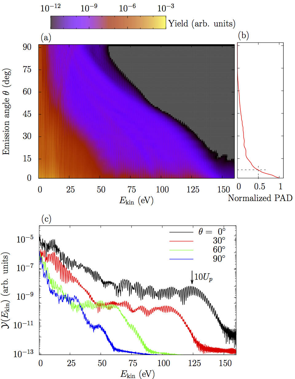
Figure 1: (a): Color map of angle-resolved photo-electron spectra (ARPES) as a function of kinetic energy and emission angle, in logarithmic scale for the yield, from $\text{C}_{60}$ excited by a laser pulse with following parameters : $\omega_{\text{las}}=1.36$ eV, $T_{\rm pulse}=24$ fs, $I_{\mathrm{las}}=1.6\times{10}^{14}\leavevmode\nobreak\ \text{W}/\text{cm}^{2}$. (b): PAD obtained from integration of the ARPES over the high-energy range of [50–160 eV], normalized to 1 at $0\mathrm{{}^{\circ}}$. The dashed line marks the cone angle at full width at half maximum. (c): PES for emission angles at $\theta=0\mathrm{{}^{\circ}},30\mathrm{{}^{\circ}},60\mathrm{{}^{\circ}},\rm{and}\leavevmode\nobreak\ 90\mathrm{{}^{\circ}}$ (in logarithmic scale), with an arrow indicating the $10U_{p}$ cutoff energy.

The ARPES clearly indicates that electron emission is more pronounced for higher energies and is strongly focused in forward direction ($\theta=0\mathrm{{}^{\circ}}$) : The ratio of the yield at $0\mathrm{{}^{\circ}}$ and at $90\mathrm{{}^{\circ}}$ increases from $\sim 100$ at low energies to $\sim 10^{5}$ in the high energy range (100–150 eV). Analyzing the angular distributions in Fig. 1 (b) yields a focusing of $\sim{7}\mathrm{{}^{\circ}}$ (full width at half maximum), similar to values observed in gold nanotips  Park et al. (2012).

In Fig. 1(c), we present the photoelectron spectra for different emission angles, as indicated. All four PES start with a nearly exponential decrease and then, for higher energies, develop into a broad plateau which extends up to a distinct cut-off. We will discuss this structure in more details in the next section. Note that this typical pattern is well known and can be qualitatively understood by the so called “three-step model” Corkum (1993): the electron is ionized during the laser field through tunnel ionization, then accelerated in the electric field, driven back to the ion core and gains a large amount of energy through recollision with the latter. Within this simple picture, the cut-off appears at $\sim 10U_{p}$ with $U_{p}=\frac{I_{\mathrm{las}}}{4\,\omega_{\text{las}}^{2}}$ being the ponderomotive energy. Here, the angular dependence of the cut-off roughly follows a $\cos\theta$ dependence, similar to the angular tendency of cut-off shown in Paulus et al. (1994); Cornaggia (2008). A further interesting finding is the oscillatory structure of the PES within the high energy plateau. Similar structures have been observed in other systems Kopold and Becker (1999); Frolov et al. (2009), where they were interpreted as interference effects of different electron trajectories leading to the same final kinetic energy. In Sec. C, we will analyze the time evolution of the spectra, and we will show that this interpretation is consistent with our results. In the following section, we will first address the intensity dependence of the photoelectron spectra.

III.2 Impact of laser intensity

III.2.1 PES as a function of laser intensity

To study the influence of the laser intensity on PES of irradiated $\text{C}_{60}$, four intensities have been explored, namely $I_{0}$, 2$I_{0}$, 4.6$I_{0}$, and $8I_{0}$ where $I_{0}=2\times 10^{13}\leavevmode\nobreak\ \text{W}/\text{cm}^{2}$, corresponding to values of the Keldysh parameter $\gamma=1.5$, 1.1, 0.7, and 0.5 respectively. Figure 2 collects the results for the PES in forward direction ($\theta=0\mathrm{{}^{\circ}}$).

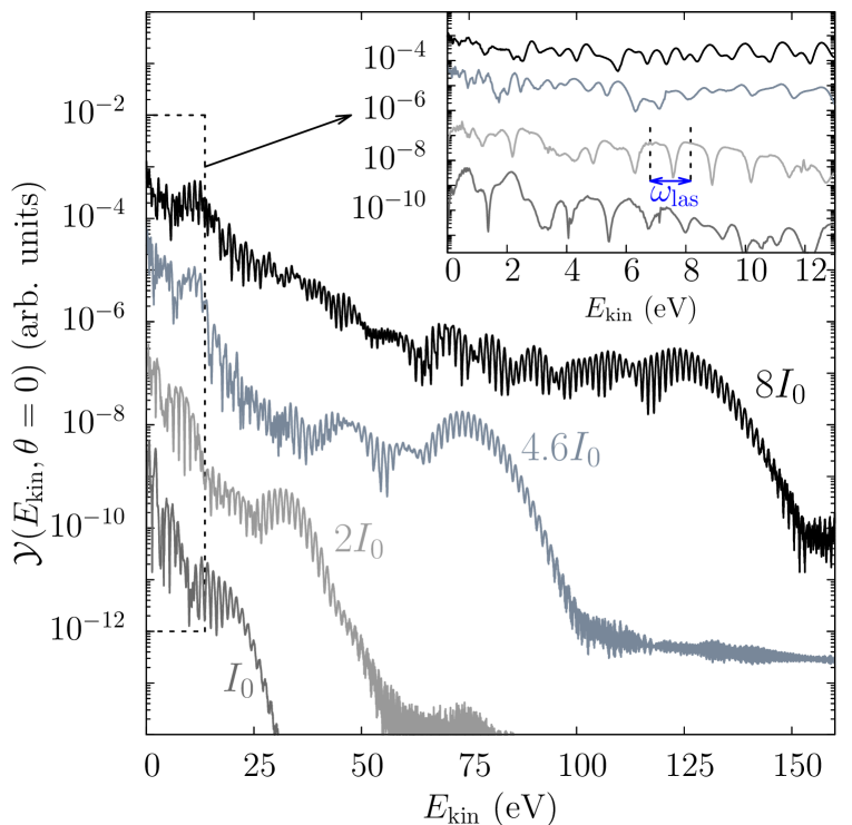
Figure 2: Samples of photo-electron spectra in forward direction in $\text{C}_{60}$ irradiated by laser pulses with $\omega_{\text{las}}=1.36$ eV (912 nm), $T_{\rm pulse}=24$ fs, and four intensities as indicated ($I_{0}=2\times 10^{13}\leavevmode\nobreak\ \text{W}/\text{cm}^{2}$). The curves are vertically shifted for a better graphical discrimination. Inset : zoom in the region $0<E_{\mathrm{kin}}<13$ eV contributed by direct emissions.

They exhibit similar pattern at all four considered intensities : on the low-energy side, they show a more or less extended plateau (see inset), then turn to a rapid exponential decrease, and finally develop a broad second plateau which extends to high energies. Both plateaus are shifted towards higher kinetic energy with increasing laser intensity, whereby the width of the plateau increases as well and thus the upper energy cut-off of the second plateau increases accordingly.

We first concentrate on the PES at low energies ($<13$ eV) magnified in the inset of Fig. 2. For the two lowest intensities ($I_{0}$ and $2I_{0}$), they show a dense sequence of peaks which are separated by the photon energy $\omega_{\text{las}}=1.36\leavevmode\nobreak\ \rm{eV}$. This is the typical pattern for Above-Threshold Ionization (ATI), which has been well studied for $\text{C}_{60}$ experimentally Campbell et al. (2000); Kjellberg et al. (2010) and theoretically Pohl et al. (2004); Wopperer et al. (2015a); Gao et al. (2015). These equi-spaced patterns are washed out when the laser intensity increases to the two highest values ($4.6\,I_{0}$, $8\,I_{0}$). This can have several reasons: first, due to the significant ionization at these intensities, the cluster progressively becomes charged during the laser pulse, leading to changes in the electronic structure. This effect has been observed in sodium clusters, see e.g. Pohl et al. (2000, 2004), and preliminary investigations have clearly shown similar effects in the present case too. However, additional blurring due to other effects, like the space charge, may also contribute, and will be analyzed in future studies.

III.2.2 Analysis of the high energy plateau

As mentioned above, the high-energy plateau is generated by strong-field ionization (SFI) mechanism, and the characteristic cut-offs can be found approximately at $10.007\leavevmode\nobreak\ U_{p}$ Paulus et al. (1994). Moreover, the derivation of a semiclassical cut-off law Busuladžić et al. (2006), based on the Strong Field Approximation (SFA), reveals that the IP also plays a role in the SFI regime, and can be estimated by Busuladžić et al. (2006):

$$E_{\mathrm{cut}}^{\mathrm{(SFA)}}=10.007\,U_{p}+0.538\,E_{\mathrm{IP}}\;,\ U_{p}=\frac{I_{\mathrm{las}}}{4\,\omega_{\text{las}}^{2}}\;,$$ (8)

Because of the inverse quadratic dependence of $U_{p}$ on the laser frequency $\omega_{\text{las}}$, the low value of 1.36 eV used here delivers a large ponderomotive energy and large cut-offs in the PES. For instance, at 4.6$I_{0}$, we have $U_{p}$=7.1 eV, largely exceeding the photon energy and being even comparable to $E_{\mathrm{IP}}$, and $E_{\mathrm{cut}}^{\mathrm{(SFA)}}=75$ eV in Fig. 2.

We have extracted the energy cut-off from our calculated PES, denoted by $E_{\rm cut}^{({\rm TDLDA})}$ to compare it to the simple estimate $E_{\rm cut}^{({\rm SFA})}$ given by Eq. (8). More precisely, for a given PES, $E_{\rm cut}^{({\rm TDLDA})}$ is obtained as the intersect of two fitting exponential curves at each side of the plateau, similarly to the procedure applied on experimental data Krüger et al. (2011). The comparison of $E_{\rm cut}^{({\rm TDLDA})}$ and $E_{\rm cut}^{({\rm SFA})}$ is presented in Fig. 3.

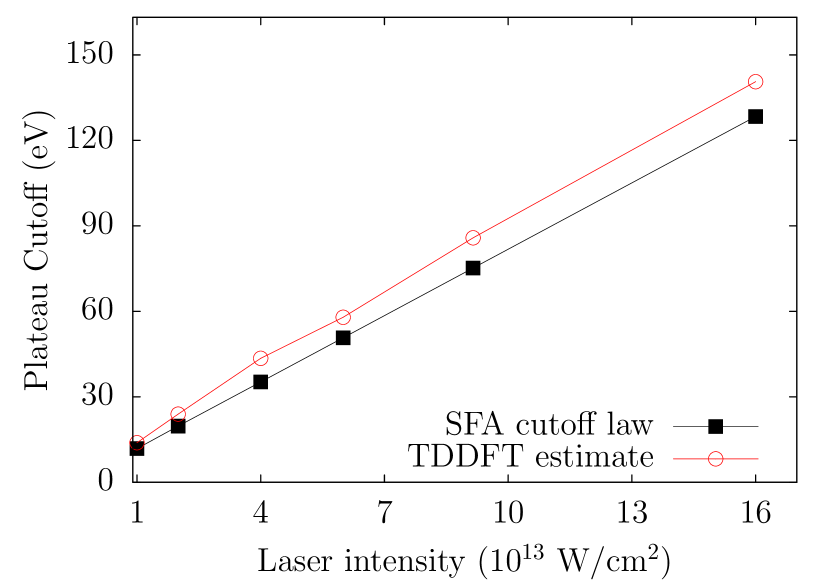
Figure 3: Cutoff energies of the high-energy plateau in the PES as functions of the laser intensity, from TDLDA calculations compared with the estimate (8) deduced from the strong field approximation (SFA).

We first note that both energy cut-offs grow linearly with laser intensity, pointing towards the validity of the simple classical scaling law. However, our numerical simulations show a slightly steeper slope. If one interprets the numerical results obtained by the TDLDA approach in the light of the simple classical scaling law (8), the difference may be explained by a field enhancement of about 5 to $10\%$. Further investigations are needed to confirm this interpretation. Note however that a similar effect has been observed in metallic nanotips Schenk et al. (2010); Park et al. (2012); Krüger et al. (2012b).

III.2.3 Ponderomotive oscillations

To better visualize the ponderomotive motion, we show in the lower panels of Fig. 4 the current density $j_{z}$ along the laser polarization axis $z$.

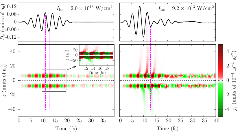
Figure 4: Electronic dipole moment $D_{z}$ as a function of time (top row), and current density $j_{z}$ as a function of time and $z$ coordinate (bottom row, 2D density map) of C₆₀ along laser polarization axis ($z$ direction), after irradiation by a laser pulse with $\omega_{\text{las}}=1.36$ eV, $T_{\rm pulse}=24$ fs, and with two different intensities $I_{\text{las}}=2.0\times 10^{13}\leavevmode\nobreak\ \text{W}/\text{cm}^{2}$ (left column) and $I_{\text{las}}=9.2\times 10^{13}\leavevmode\nobreak\ \text{W}/\text{cm}^{2}$ (right column). Positive $j_{z}$ are depicted in red (or gray), and negative $j_{z}$ are in green (or light gray). For a given color (or type of gray), the brighter the shade, the smaller the absolute value of $j_{z}$. The inset in the left bottom panel magnifies the map between 10 and 20 fs with a scale in current density divided by 100.

Two intensities are considered, one at the moderate side with $I_{\text{las}}=I_{0}=2\times 10^{13}\leavevmode\nobreak\ \text{W}/\text{cm}^{2}$ (left column) and another one at higher intensity of $I_{\text{las}}=4.6\,I_{0}=9.2\times 10^{13}\leavevmode\nobreak\ \text{W}/\text{cm}^{2}$ (right column). The current density is plotted in a 2D density map as a function of time (horizontal axis) and space coordinate $z$ (vertical axis), with positive $j_{z}$ in red (or gray) and negative $j_{z}$ in green (or light gray). It is also instructive to compare these maps with the time evolution of the dipole moment defined in Eq. (6) which is plotted in the top panel of the figure. Note that the dipole moment and the current density are related by the continuity equation which reads :

$$\frac{\partial D_{z}}{\partial t}=\int_{z}\textrm{d}z\leavevmode\nobreak\ j_{z}\;.$$ (9)

The sign of the time derivative of $D_{z}$ is thus equal to the one of the dominant part of $j_{z}$.

One observes successive fringes in $j_{z}$ connected to the change of sign of the derivative of $D_{z}$ or, in other words, to the oscillations of $D_{z}$ in time, as exemplified by vertical dashes in a case when the sign is negative. For the highest laser intensity (right column of Fig. 4), a sizable backflow of the current density occurs during pulse duration, especially between 5 and 15 fs, where the field amplitude is maximal. For instance, in the time interval indicated by the two vertical dashed lines, the majority of electrons possess a negative $j_{z}$ (they are thus pulled away from the $\text{C}_{60}$), while a non-negligible amount exhibits a positive $j_{z}$, which means that they are pulled back towards $\text{C}_{60}$ and that recollision is possible. At the lowest $I_{\mathrm{las}}$, this backflow still exists but is much weaker, see inset in the bottom left panel for which the current density scale has been divided by 100 to allow the visualization of this weak counterflow. The amplitude of this quiver motion can be estimated from a purely classical model as $l_{\mathrm{q}}=\alpha E_{0}/\omega^{2}$ where $\alpha$ is the field enhancement factor (here about 1.05). This yields $l_{\mathrm{q}}\sim 12\leavevmode\nobreak\ \mathrm{a}_{0}$ and $\sim 25\leavevmode\nobreak\ \mathrm{a}_{0}$ at the low and the high $I_{\mathrm{las}}$ respectively. These classical $l_{\mathrm{q}}$ agree well with the amplitudes one can read off from the current density maps. The large ponderomotive oscillations terminate as soon as the external field dies out. The further evolution still shows a succession of positive and negative fringes of $j_{z}$, but electrons in the $z>0$ and the $z<0$ regions do not oscillate in phase anymore. This is particularly visible for the highest $I_{\mathrm{las}}$ above 20 fs.

III.3 Time-resolved analysis

As mentioned above, in addition to the high-energy cut-off, we see modulations of the PES within the broad plateau for the two cases with the higher intensities in Fig. 2. Similar structures have been experimentally observed in the photoemission spectra of rare gases (i.e., argon atom Paulus et al. (2001)) ionized by strong infrared laser pulses. These structures have been interpreted as interference effects from several electron trajectories generated either in the same optical cycle or in the subsequent optical cycle, leading to the same final states  Lewenstein et al. (1994). In particular, in this work, two types of trajectories have been identified, labeled as “short” and “long” trajectories, due to their different excursion times. Within the three-step model, the electrons are born close to the field maxima, where the tunnel ionization probability is maximal.

Since we focus on electron emission in the forward direction, we have chosen, for the time-resolved analysis, instants based on a classical picture of the electron emission. More precisely, the “birth” times of the electrons, denoted by $t_{\rm b1/2/3}$, are taken at the three largest maxima of the electric force, that is at respectively 2.75, 3.75, and 4.75 $t_{\mathrm{oc}}$, where $t_{\mathrm{oc}}=3$ fs is the single optical cycle. We have indicated these birth times in Fig. 5(a). We then correlate $t_{\rm b1/2/3}$ with the detection time $t_{\rm f1/2/3}$. Since the (fastest) electrons generated at $t_{\rm b}$ need time to reach the boundary where they are detected, we take into account a time delay $\Delta t$ which consists of two terms. The first one is the “return” time for the electron to recollide with the target and is about $0.75t_{\mathrm{oc}}$. The second one is the time for electrons emitted from the rescattering site to travel to the detection points $R_{b}=90\leavevmode\nobreak\ \mathrm{a}_{\rm 0}$ near the boundary of the simulation box. This “traveling” time is $(R_{b}-R)$/$\sqrt{2E_{\mathrm{kin}}}$ for electrons recorded with kinetic energy $E_{\mathrm{kin}}$. All in all, we have used :

$$t_{f} \approx t_{b}+\Delta t,$$ (10a)

$$\Delta t = 0.75t_{\mathrm{oc}}+(R_{b}-R)/\sqrt{2E_{\mathrm{kin}}}.$$ (10b)

For $t_{\rm b1}$, we used $E_{\mathrm{kin}}=70$ eV leading to $\Delta t=1.04\leavevmode\nobreak\ t_{\mathrm{oc}}$, while for $t_{\rm b2}$ and $t_{\rm b3}$, we took $E_{\mathrm{kin}}=135$ eV and then obtained $\Delta t=0.96\leavevmode\nobreak\ t_{\mathrm{oc}}$. Plugging these numbers in Eqs. (10), we got $t_{\rm f1/2/3}=$ 3.79, 4.71, and 5.71 $t_{\mathrm{oc}}$ respectively, as symbolized in Fig. 5(b).

The bottom panel of Fig. 5 presents three different PES, note that each one has been analyzed from $t=0$ up to one of the “final” times introduced above.

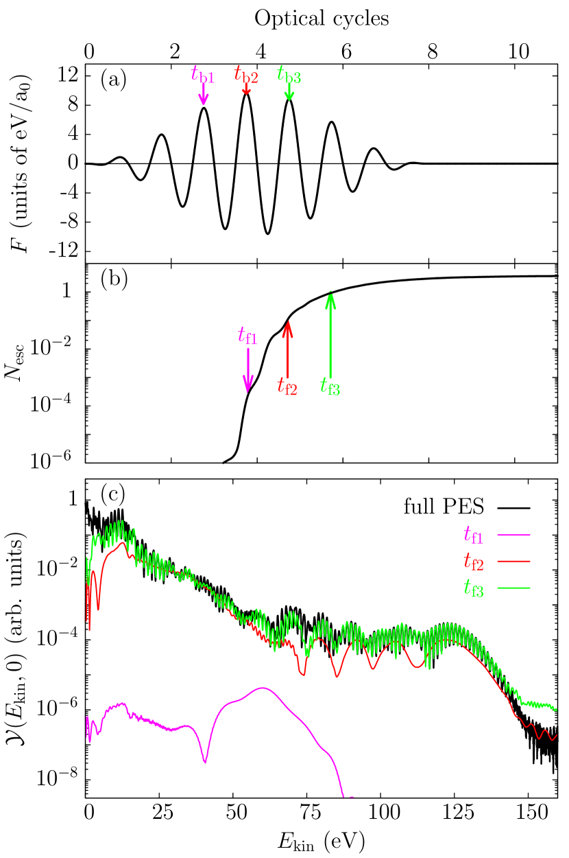
Figure 5: Time-resolved analysis of photo-emission from $\text{C}_{60}$ irradiated by a laser pulse polarized in the $z$ direction, with $\omega_{\text{las}}=1.36$ eV, $T_{\rm pulse}=24$ fs and $I_{\mathrm{las}}=1.6\times{10}^{14}\leavevmode\nobreak\ \text{W}/\text{cm}^{2}$. (a) Time evolution of the force $F$ acting on electrons, with 3 “birth” times indicated by arrows (see text for details). (b) Time evolution of the total ionization $N_{\text{esc}}$, with 3 “final” times indicated by arrows and defined in Eqs. (10). (c) Full PES (black) and PES from data accumulated up to the 3 different final times.

In addition, the full PES (black curve) obtained at the end of the laser pulse is shown. We can therefore progressively observe how the full PES builds up in time. It should be noted that this analysis is strictly valid only for the high-energy electrons, since low-energy electrons arrive later, and are thus not accounted for at the corresponding final times $t_{\rm f1/2/3}$.

As a first result, we see that the spectra at $t_{\rm f1}$ is about two to three orders of magnitude smaller than the spectra at later times (also see the corresponding ionization in Fig.5(b)), showing that these contributions are negligible. Indeed, at the field maximum indicated by $t_{\rm b1}$, on the rising part of the pulse envelop, the field strength is not yet sufficient for an efficient tunnel ionization. The major part of the spectrum, containing the main structures, is obtained for the spectrum at $t_{\rm f2}$, which corresponds to a birth time $t_{\rm b2}$ at the highest field value of the pulse. It shows a clear plateau, with distinct modulations. If one interprets these structures as interferences from two electron trajectories, it would correspond to a relative phase of $\delta S=E_{\mathrm{kin}}\delta t$ Milošević et al. (2006) with $\delta t$=0.41 fs, well below the optical period $t_{\mathrm{oc}}$= 3 fs. This value of $\delta t$, about one seventh of $t_{\rm oc}$, is in the same order as deduced by an extended schematic model for recent laser-nanotip interactions, estimated to about one sixth in this case Krüger et al. (2012b). Within this interpretation of interference of different electron trajectories, the findings of the numerically calculated spectra at $t_{\rm f2}$ would correspond to “intracycle” interferences, i.e., interference that stems from electron trajectories originating during the same optical period. When comparing to the spectrum at $t_{\rm f3}$, one sees that the additional changes with respect to that at $t_{\rm f2}$ are minor at the side of the extension of the plateau, however, one striking difference can be observed: the appearance of high-frequency modulations in the spectra. These modulations correspond to peaks separated by the central frequency $\omega_{\mathrm{las}}$. From a temporal point of view, these structures are created by interferences of electron trajectories that are born at times separated by the optical period, and can thus be identified as “intercycle” interferences. These are commonly observed for longer pulses, where several field peaks have comparable maxima, as it is in the present case.

When compared to the full spectra, one sees slow convergence for the low-energy electrons. This can be understood by the fact that these electrons, due to their slower speed, only arrive at delays much larger than $\Delta t$. This systematic effect is clearly visible in all time-resolved spectra.

To summarize, we have analyzed the time evolution of the spectra obtained by the fully numerical TDDFT calculations by choosing particular detection times to separate as fully as possible the contributions from the different field maxima. While not claiming to have unambiguously identified the observed structures, we have shown that their characteristics, both in their time evolution as well as with respect to their frequency fingerprints, are consistent with the picture of interfering intra- and intercycle trajectories.

IV Conclusions

In this paper, we have analyzed the electron dynamics of laser-excited $\text{C}_{60}$ as a model case for the generation of high-energy electrons from a carbon tip. We have explored the response of the system to laser fields of various intensities for a frequency in the infrared domain which leads, at high intensities, to significant ponderomotive effects. To analyze such a complex dynamics, we go beyond single-active-electron approaches and use time-dependent density-functional theory propagated in real time and computed on a spatial grid. This approach allows, in particular, a proper description of collective electronic motion as well as a detailed analysis of photo-electron spectra (PES) and photo-angular distributions (PAD). One of the main numerical challenges in the present investigation was the large box size required to account for the huge pathway of the ponderomotive motion of the electrons. To make that feasible in a quantum mechanical framework, we use a spherical jellium approximation for the ionic background and handle the dynamics on a cylindrical grid.

As a major result, we have shown that the recollision regime can be reached for strong, but realistic, laser intensities. We find the establishment of a plateau stretching out to very high kinetic energies, e.g. to about 125 eV for $I=1.6\times 10^{14}$ W/cm², which is interpreted using the well-known recollision mechanism and illustrated by using a map of the time dependence of the current distribution. The cut-off of the plateau is shown to follow the semiclassical model based on the three-step model, with a field which is enhanced by about $10\%$ in our simulations. A detailed time-resolved analysis of the PES demonstrates how the high-energy plateau is generated successively during the laser pulse. In particular, we have shown that the observed structures and their time evolution stemming from different peaks of the field are consistent with the picture of intra- and intercycle interferences. As far as the angular distribution is concerned, one of the most promising results of the presented study is the strong focusing of the electrons in the forward direction, especially for the high energy electrons provided by the recollision process. This is an important feature in the context of using carbon nanotubes as future sources of collimated electron beams for time-resolved diffraction experiments.

References

- Hilbert et al. (2009) S. Hilbert, A. Neukirch, C. Uiterwaal, and H. Batelaan, J. Phys. B: At., Mol. Opt. Phys. 42, 141001 (2009).
- Williamson et al. (1997) J. C. Williamson, J. Cao, H. Ihee, H. Frey, and A. H. Zewail, Nature 386, 159 (1997).
- Lobastov et al. (2005) V. A. Lobastov, R. Srinivasan, and A. H. Zewail, Proc. Natl. Acad. Sci. U. S. A. 102, 7069 (2005).
- Paul et al. (2001) P. M. Paul, E. S. Toma, P. Breger, G. Mullot, F. Augé, P. Balcou, H. G. Muller, and P. Agostini, Science 292, 1689 (2001).
- Agostini and DiMauro (2004) P. Agostini and L. F. DiMauro, Rep. Prog. Phys. 67, 813 (2004).
- Bormann et al. (2010) R. Bormann, M. Gulde, A. Weismann, S. V. Yalunin, and C. Ropers, Phys. Rev. Lett. 105, 147601 (2010).
- Schenk et al. (2010) M. Schenk, M. Krüger, and P. Hommelhoff, Phys. Rev. Lett. 105, 257601 (2010).
- Krüger et al. (2012a) M. Krüger, M. Schenk, P. Hommelhoff, G. Wachter, C. Lemell, and J. Burgdörfer, New J. Phys. 14, 085019 (2012a).
- Carroll et al. (1997) D. L. Carroll, P. Redlich, P. M. Ajayan, J. C. Charlier, X. Blase, A. De Vita, and R. Car, Phys. Rev. Lett. 78, 2811 (1997).
- Saito et al. (1997) Y. Saito, K. Hamaguchi, K. Hata, K. Uchida, Y. Tasaka, F. Ikazaki, M. Yumura, A. Kasuya, and Y. Nishina, Nature 389, 554 (1997).
- Nilius et al. (2000) N. Nilius, N. Ernst, and H.-J. Freund, Phys. Rev. Lett. 84, 3994 (2000).
- Bionta et al. (2014) M. Bionta, B. Chalopin, A. Masseboeuf, and B. Chatel, Ultramicroscopy (2014), in press.
- Saito et al. (1992) R. Saito, M. Fujita, G. Dresselhaus, and M. S. Dresselhaus, Phys. Rev. B 46, 1804 (1992).
- Kawashita et al. (2009) Y. Kawashita, T. Nakatsukasa, and K. Yabana, J. Phys. Condens. Matter 21, 064222 (2009).
- Fennel et al. (2010) T. Fennel, K.-H. Meiwes-Broer, J. Tiggesbäumker, P. M. Dinh, P.-G. Reinhard, and E. Suraud, Rev. Mod. Phys. 82, 1793 (2010).
- Runge and Gross (1984) E. Runge and E. K. U. Gross, Phys. Rev. Lett. 52, 997 (1984).
- Dreizler and Gross (1990) R. M. Dreizler and E. K. U. Gross, Density Functional Theory: An Approach to the Quantum Many-Body Problem (Springer-Verlag, Berlin, 1990).
- Perdew and Wang (1992) J. P. Perdew and Y. Wang, Phys. Rev. B 45, 13244 (1992).
- Kroto et al. (1985) H. W. Kroto, J. R. Heath, S. C. O’Brien, R. F. Curl, and R. E. Smalley, Nature 318, 162 (1985).
- Puska and Nieminen (1993) M. J. Puska and R. M. Nieminen, Phys. Rev. A 47, 1181 (1993).
- Bauer et al. (2001) D. Bauer, F. Ceccherini, A. Macchi, and F. Cornolti, Phys. Rev. A 64, 063203 (2001).
- Cormier et al. (2003) E. Cormier, P.-A. Hervieux, R. Wiehle, B. Witzel, and H. Helm, Eur. Phys. J. D 26, 83 (2003).
- Reinhard et al. (2013) P.-G. Reinhard, P. Wopperer, P. M. Dinh, and E. Suraud, in ICQNM 2013, The Seventh International Conference on Quantum, Nano and Micro Technologies (2013), pp. 13–17.
- Hedberg et al. (1991) K. Hedberg, L. Hedberg, D. S. Bethune, C. Brown, H. Dorn, R. D. Johnson, and M. De Vries, Science 254, 410 (1991).
- Madjet et al. (2008) M. E. Madjet, H. S. Chakraborty, J. M. Rost, and S. T. Manson, J. Phys. B: At., Mol. Opt. Phys. 41, 105101 (2008).
- Lichtenberger et al. (1990) D. L. Lichtenberger, M. E. Jatcko, K. W. Nebesny, C. D. Ray, D. R. Huffman, and L. D. Lamb, Mater. Res. Soc. Symp. Proc. 206, 673 (1990).
- Sattler (2010) K. Sattler, Handbook of Nanophysics: Clusters and Fullerenes, Handbook of Nanophysics (CRC Press, 2010).
- Korica et al. (2010) S. Korica, A. Reinköster, M. Braune, J. Viefhaus, D. Rolles, B. Langer, G. Fronzoni, D. Toffoli, M. Stener, P. Decleva, et al., Surf. Sci. 604, 1940 (2010).
- Toffoli and Decleva (2010) D. Toffoli and P. Decleva, Phys. Rev. A 81, 061201(R) (2010).
- Araidai et al. (2004) M. Araidai, Y. Nakamura, and K. Watanabe, Phys. Rev. B 70, 245410 (2004).
- Driscoll et al. (2011) J. A. Driscoll, B. Cook, S. Bubin, and K. Varga, J. Appl. Phys. 110, 024304 (2011).
- Wopperer et al. (2015a) P. Wopperer, P. M. Dinh, P.-G. Reinhard, and E. Suraud, Phys. Rep. 562, 1 (2015a).
- Gao et al. (2015) C.-Z. Gao, P. Wopperer, P. M. Dinh, P.-G. Reinhard, and E. Suraud, J. Phys. B: At., Mol. Opt. Phys. 48, 105102 (2015).
- Wopperer et al. (2015b) P. Wopperer, C. Z. Gao, T. Barillot, C. Cauchy, A. Marciniak, V. Despré, V. Loriot, G. Celep, C. Bordas, F. Lépine, et al., Phys. Rev. A 91, 042514 (2015b).
- Herink et al. (2012) G. Herink, D. Solli, M. Gulde, and C. Ropers, Nature 483, 190 (2012).
- Wopperer et al. (2010a) P. Wopperer, B. Faber, P. M. Dinh, P.-G. Reinhard, and E. Suraud, Phys. Lett. A 375, 39 (2010a).
- Wopperer et al. (2010b) P. Wopperer, B. Faber, P. M. Dinh, P.-G. Reinhard, and E. Suraud, Phys. Rev. A 82, 063416 (2010b).
- Ashcroft and Mermin (1976) N. W. Ashcroft and N. D. Mermin, Solid State Physics (Saunders College, Philadelphia, 1976).
- Ekardt (1984) W. Ekardt, Phys. Rev. Lett. 52, 1925 (1984).
- Brack (1993) M. Brack, Rev. Mod. Phys. 65, 677 (1993).
- Gunnarsson et al. (1995) O. Gunnarsson, H. Handschuh, P. S. Bechthold, B. Kessler, G. Ganteför, and W. Eberhardt, Phys. Rev. Lett. 74, 1875 (1995).
- Reinhard and Suraud (2015) P.-G. Reinhard and E. Suraud, Ann. Phys. (N.Y.) 354, 183 (2015).
- Keldysh (1965) L. V. Keldysh, Sov. Phys. JETP 20, 1307 (1965).
- Mevel et al. (1993) E. Mevel, P. Breger, R. Trainham, G. Petite, P. Agostini, A. Migus, J.-P. Chambaret, and A. Antonetti, Phys. Rev. Lett. 70, 406 (1993).
- Li et al. (2015) H. Li, B. Mignolet, G. Wachter, S. Skruszewicz, S. Zherebtsov, F. Süßmann, A. Kessel, S. A. Trushin, N. G. Kling, M. Kübel, et al., Phys. Rev. Lett. 114, 123004 (2015).
- Calvayrac et al. (2000) F. Calvayrac, P.-G. Reinhard, E. Suraud, and C. A. Ullrich, Phys. Rep. 337, 493 (2000).
- Reinhard and Suraud (2003) P.-G. Reinhard and E. Suraud, Introduction to Cluster Dynamics (Wiley, New York, 2003).
- Reinhard and Cusson (1982) P.-G. Reinhard and R. Y. Cusson, Nucl. Phys. A 378, 418 (1982).
- Feit et al. (1982) M. D. Feit, J. A. Fleck, and A. Steiger, J. Comp. Phys. 47, 412 (1982).
- Calvayrac et al. (1997) F. Calvayrac, E. Suraud, and P.-G. Reinhard, Ann. Phys. (N.Y.) 255, 125 (1997).
- Pohl et al. (2000) A. Pohl, P.-G. Reinhard, and E. Suraud, Phys. Rev. Lett. 84, 5090 (2000), URL http://link.aps.org/doi/10.1103/PhysRevLett.84.5090.
- Pohl et al. (2001) A. Pohl, P.-G. Reinhard, and E. Suraud, J. Phys. B 34, 4969 (2001).
- Dinh et al. (2013) P. M. Dinh, P. Romaniello, P.-G. Reinhard, and E. Suraud, Phys. Rev. A 87, 032514 (2013).
- Park et al. (2012) D. J. Park, B. Piglosiewicz, S. Schmidt, H. Kollmann, M. Mascheck, and C. Lienau, Phys. Rev. Lett. 109, 244803 (2012).
- Corkum (1993) P. B. Corkum, Phys. Rev. Lett. 71, 1994 (1993).
- Paulus et al. (1994) G. G. Paulus, W. Becker, W. Nicklich, and H. Walther, J. Phys. B: At., Mol. Opt. Phys. 27, L703 (1994).
- Cornaggia (2008) C. Cornaggia, Phys. Rev. A 78, 041401 (2008).
- Kopold and Becker (1999) R. Kopold and W. Becker, J. Phys. B: At., Mol. Opt. Phys. 32, L419 (1999).
- Frolov et al. (2009) M. V. Frolov, N. L. Manakov, and A. F. Starace, Phys. Rev. A 79, 033406 (2009).
- Campbell et al. (2000) E. E. B. Campbell, K. Hansen, K. Hoffmann, G. Korn, M. Tchaplyguine, M. Wittmann, and I. V. Hertel, Phys. Rev. Lett. 84, 2128 (2000).
- Kjellberg et al. (2010) M. Kjellberg, O. Johansson, F. Jonsson, A. V. Bulgakov, C. Bordas, E. E. B. Campbell, and K. Hansen, Phys. Rev. A 81, 023202 (2010).
- Pohl et al. (2004) A. Pohl, P.-G. Reinhard, and E. Suraud, J. Phys. B 37, 3301 (2004).
- Busuladžić et al. (2006) M. Busuladžić, A. Gazibegović-Busuladžić, and D. Milošević, Laser Phys. 16, 289 (2006).
- Krüger et al. (2011) M. Krüger, M. Schenk, and P. Hommelhoff, Nature 475, 78 (2011).
- Krüger et al. (2012b) M. Krüger, M. Schenk, M. Förster, and P. Hommelhoff, J. Phys. B: At., Mol. Opt. Phys. 45, 074006 (2012b).
- Paulus et al. (2001) G. G. Paulus, F. Grasbon, H. Walther, R. Kopold, and W. Becker, Phys. Rev. A 64, 021401 (2001).
- Lewenstein et al. (1994) M. Lewenstein, P. Balcou, M. Y. Ivanov, A. L’Huillier, and P. B. Corkum, Phys. Rev. A 49, 2117 (1994).
- Milošević et al. (2006) D. Milošević, G. Paulus, D. Bauer, and W. Becker, J. Phys. B: At., Mol. Opt. Phys. 39, R203 (2006).