The accuracy of telling time via oscillatory signals

Abstract

Circadian clocks are the central timekeepers of life, allowing cells to anticipate changes between day and night. Experiments in recent years have revealed that circadian clocks can be highly stable, raising the question how reliably they can be read out. Here, we combine mathematical modeling with information theory to address the question how accurately a cell can infer the time from an ensemble of protein oscillations, which are driven by a circadian clock. We show that the precision increases with the number of oscillations and their amplitude relative to their noise. Our analysis also reveals that their exists an optimal phase relation that minimizes the error in the estimate of time, which depends on the relative noise levels of the protein oscillations. Lastly, our work shows that cross-correlations in the noise of the protein oscillations can enhance the mutual information, which suggests that cross-regulatory interactions between the proteins that read out the clock can be beneficial for temporal information transmission.

Introduction

Among the most fascinating timing devices in biology are circadian clocks, which are found in organisms ranging from cyanobacteria and fungi, to plants, insects and animals. Circadian clocks are biochemical oscillators that allow organisms to coordinate their behavior with the 24-hour cycle of day and night. Remarkably, these clocks can maintain stable rhythms for months or even years in the absence of any daily cue from the environment, such as light/dark or temperature cycles Johnson2008 . In multicellular organisms, the robustness can be explained by intercellular interactions Liu:1997uv ; Yamaguchi:2003jj , but it is now known that even unicellular organisms can have very stable rhythms. An excellent example is provided by the clock of the bacterium Synechococcus elongatus, which is one of the most studied and best characterized model systems Johnson2008 . This clock has a correlation time of several months Mihalcescu:2004ch , even though the clocks of the different cells in the population do not seem to interact with one another Mihalcescu:2004ch . Clearly, the clock is designed in such a way that it has become resilient against the intrinsic stochasticity of the chemical reactions that constitute the clock Zwicker2010 ; Paijmans2015 . The observation that clocks can be very stable, suggests that they are also read out reliably. Yet, how cells could do so is a wide open question Mugler:2010cq .

In this manuscript we combine information theory with mathematical modeling to study how accurately cells can infer time from cellular oscillators. While our analysis is general, it is inspired by the circadian clock of S. elongatus. The central clock component of S. elongatus is KaiC, which forms a hexamer Kageyama2003 . KaiC has two phosphorylation sites per monomer, which are phosphorylated and dephosphorylated in a well-defined temporal order, yielding a protein-phosphorylation cycle (PPC) with a 24 hour period Rust2007 ; Nishiwaki2007 . This PPC is coupled to a transcription-translation cycle (TTC) of KaiC Kitayama2008 , which is a protein synthesis cycle with a 24 hr rhythm, via the response regulator RpaA. KaiC in the phosphorylation phase of the PPC activates the histidine kinase SasA, which in turn activates RpaA via phosphorylation Takai2006 ; Taniguchi:2007jx ; Taniguchi2010 ; Gutu2013 . In contrast, KaiC that is in the dephosphorylation phase of the PPC and bound to KaiB, activates the phosphatase CikA, which dephosphorylates and deactivates RpaA Taniguchi2010 ; Gutu2013 . Active, phosphorylated RpaA drives genome-wide transcriptional rhythms, which include the expression of the clock components Markson2013 .

Intriguingly, while time could be uniquely encoded in the modification state of the two phosphorylation sites of KaiC, cells do not seem to employ this mechanism Gutu2013 ; Markson2013 . RpaA, the central node between the clock and the downstream genes, has only one phosphorylation site Gutu2013 ; Markson2013 . This makes the question how accurately the cell can infer time a very pertinent one, because a single readout—the phoshorylation level of RpaA—leads to an inherent ambiguity in the mapping between time and clock output: a given level of active RpaA corresponds to two possible times (see Fig. 1). On the other hand, it is known that RpaA controls the expression of many downstream genes Markson2013 . While their expression levels cannot contain more information about time than that which is available in the time trace of RpaA, it is possible that, collectively, their expression levels do contain more information about time than that present in the instantaneous level of RpaA.

In this manuscript, we study how the accuracy of telling time depends on the number of genes that read out a clock, their phase difference, the level of biochemical noise, and the cross-correlations between the gene expression levels. In the next section, we first describe the set up of our analysis, and then the measures that we employ to quantify information transmision. We then show that there exists an optimal phase difference that maximizes information transmission. Interestingly, the optimal phase difference depends on the amplitude of the noise in the expression of the readout genes, and on the cross-correlations between them, akin to what has been observed in neuronal coding Tkacik2010 and in the gap-gene expression system of Drosophila Walczak:2010cv ; Dubuis2013 .

I Methods

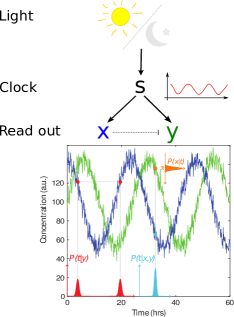
Figure 1: Cells can infer time from an ensemble of protein oscillations. The day-night rhythm entrains a circadian clock, a biochemical oscillator with a 24 hr period, which in turn drives the oscillatory expression of a number of readout genes. The precision of the estimate of time depends on the number of readout proteins, the amplitude of the oscillations, their noise level, their phase difference, and the cross-correlations in the fluctuations.

I.1 Model

The analysis we present below applies to any readout system that obeys Gaussian statistics. Yet, to set the stage, and to introduce the key quantities that we will study, it is instructive to consider a concrete system. To this end, imagine an oscillatory clock protein, like RpaA, that drives the expression of a set of downstream genes. Assuming that the system can be linearized, the dynamics of the system is given by

$$\frac{d{\bf x}(t)}{dt}={\bf f}s(t)+{\bf B}{\bf x}(t)+\xi(t).$$ (1)

Here ${\bf x}(t)$ is a vector with components $x_{i}(t)$, which denote the concentration $x_{i}$ of protein ${\rm X}_{i}$, $s(t)$ is the concentration of the clock protein, ${\bf f}$ is a vector with components $f_{i}$, which describe how the downstream protein ${\rm X}_{i}$ is driven by $s(t)$, ${\bf B}$ is the matrix that describes the regulatory interactions between the downstream proteins, and $\xi(t)$ is a vector with components $\xi_{i}(t)$ that describe the noise in the expression of ${\rm X}_{i}$. In what follows, we imagine that the clock protein osscilates according to $s(t)=A_{s}\sin(\omega t)+r_{s}+\xi_{s}$, where $A_{s}$ sets the amplitude of the oscillations, $r_{s}$ its mean, and $\xi_{s}$ describes the noise in the input signal.

This linear system can be solved analytically. For example, if the downstream genes do not interact with each other and protein ${\rm X}_{i}$ decays with rate $\mu_{i}$, then each protein oscillates as

$$x_{i}(t)=A_{i}\sin(\omega t+\phi_{i})+r_{i}+\eta_{i}(t),$$ (2)

where

$$\eta_{i}(t) = \int_{-\infty}^{t}dt^{\prime}e^{-\mu_{i}(t-t^{\prime})}\left[\xi_{i}(t^{\prime})+f_{i}\xi_{s}(t^{\prime})\right],$$ (3)

$$A_{i} = \frac{f_{i}A_{s}}{\sqrt{\mu_{i}^{2}+\omega^{2}}},$$ (4)

$$\phi_{i} = \arcsin(\frac{-\omega}{\sqrt{\mu_{i}^{2}+\omega^{2}}}),$$ (5)

$$r_{i} = \frac{f_{i}r_{s}}{\mu_{i}}.$$ (6)

Importantly, even in this simple system, the difference in the phase $\phi$ between the expression of the downstream genes can be modulated, namely by changing the protein degradation rate $\mu_{i}$. Also the amplitude $A_{i}$ can be adjusted; it can be set independently from the phase via the synthesis rate $f_{i}$. Both quantities affect the precision by which the system can estimate the time.

Another key quantity is the noise in the expression of the downstream genes. Following the linear-noise approximation, we assume that the noise in the concentration $x_{i}$ is Gaussian, such that

$$P(\eta_{i})=P(x_{i}|t^{*})=\frac{1}{\sqrt{2\pi\sigma_{i}^{2}}}e^{-\frac{({x_{i}}-\bar{x}_{i}(t^{*}))^{2}}{2\sigma_{i}^{2}}}$$ (7)

where $\bar{x}_{i}(t^{*})$ is the mean concentration of protein ${\rm X}_{i}$ at time $t^{*}$, $\sigma^{2}_{i}=\sigma^{2}_{i}(t^{*})$ is the variance of $x_{i}$ around its mean $\bar{x}_{i}$, and $t^{*}$ is the given time. The noise $\sigma^{2}_{i}(t)$ has a extrinsic contribution coming from the noise in the input signal, an intrinsic contribution from the noise in the expression of $X_{i}$, and a contribution from the regulatory interactions. Our analysis does not depend on the origins of these noise contributions: in the analysis below, we specify the variance $\sigma^{2}_{i}(t)$ and the co-variance of the fluctuations in $x_{i}$ and $x_{j}$, and then study how this affects the precision of telling time. In general, we expect, however, that $\sigma^{2}_{i}(t)$ depends on the mean $\bar{x}_{i}(t)$, and a reasonable assumption is that the variance equals the mean, $\sigma^{2}_{i}(t)=\bar{x}_{i}(t)$, as in gene expression via simple Poissonian birth-death statistics paulsson2003 . However, if the mean $r_{i}$ of the protein oscillations is large compared to their amplitude $A_{i}$, then we may assume that $\sigma^{2}_{i}(t)$ is constant in time, $\sigma^{2}_{i}(t)=\sigma^{2}_{i}=r_{i}$. As will become clear in the next section, the importance of noise depends on the amplitude of the oscillations: the key control parameter is the relative noise strength $\widetilde{\sigma}_{i}\equiv A_{i}/\sigma_{i}$. This ratio can be varied independently from gene to gene, $A_{i}/\sigma_{i}\neq A_{j}/\sigma_{j}$ in general, and below we will study how this affects the precision. If there is no noise in the input $s(t)$ and if the downstream proteins do not interact with each other (as in the example considered here), then the cross-correlation between the fluctuations of the concentrations of the downstream proteins is zero: $\langle\eta_{i}\eta_{j}\rangle=\langle\eta^{2}_{i}\rangle\delta_{ij}=\sigma^{2}_{i}$, where $\delta_{ij}$ is the Kronecker delta. However, in general, the noise in the expression of the downstream genes will be correlated, which, as we will show, can either enhance or reduce the accuracy by which the downstream proteins can infer time.

Below, we will consider how the accuracy of telling time depends on the cross-correlations between the expression of the downstream genes, their phase difference, and on $\widetilde{\sigma}_{i}$, and how this varies from gene to gene.

I.2 Reliability measures

The central idea of our analysis is that the system infers the time from the collective expression of the $N$ downstream proteins, $\{x_{i}\}\equiv\{x_{1}(t),x_{2}(t),\dots,x_{N-1}(t),x_{N}(t)\}$. Following work on positional information in Drosophila Dubuis2013 , we use two approaches to quantify the accuracy on telling time. The first is based on the error in the estimate of a given time $t$, $\sigma_{t}(t)$; a related approach has been widely used to derive the fundamental limits on the accuracy of sensing berg1977 ; Ueda:2007uq ; bialek2005 ; levinepre2007 ; levineprl2008 ; wingreen2009 ; levineprl2010 ; mora2010 ; Govern2012 ; Mehta2012 ; Skoge:2011gi ; Skoge:2013fq ; Kaizu:2014eb ; Govern:2014ef ; Govern:2014ez ; Lang:2014ir . The second approach is based on the mutual information, which in recent years has been used extensively to quantify cellular information transmission Ziv2007 ; Tostevin2009 ; Mehta2009 ; Tkacik:2009ta ; tostevin10 ; DeRonde2010 ; Tkacik2010 ; Walczak:2010cv ; DeRonde2011 ; Cheong:2011jp ; deRonde:2012fs ; Dubuis2013 ; Bowsher:2013jh ; Selimkhanov:2014gd ; DeRonde:2014fq ; Govern:2014ez ; Sokolowski:2015km ; Becker2015 .

I.2.1 The error in estimating time

To determine the error in estimating the time, we start from the generalization of Eq. 7 to multiple downstream genes:

$$P(\{x_{i}\}|t)=\frac{1}{\sqrt{2\pi|{\bf C}|}}\exp\left[-\frac{1}{2}\sum_{i,j}^{N}\delta x_{i}C^{-1}_{ij}\delta x_{j}\right].$$ (8)

Here $\delta x_{i}(t)=x_{i}(t)-\bar{x_{i}}$, ${\bf C}$ is the covariance matrix with elements $C_{ij}$, $|{\bf C}|$ is its determinant and ${\bf C}^{-1}$ is its inverse.

The idea is now to invert the problem, and ask what is the distribution of possible times $t$, given that the expression levels are $\{x_{i}\}$. This can be obtained from Bayes’ rule:

$$P(t|\{x_{i}\})=P(t)\frac{P(\{x_{i}\}|t)}{P(\{x_{i}\})}$$ (9)

where $P(t)=\frac{1}{T}$ is the uniform prior probability of having a certain time and $P(\{x_{i}\})$ is the joint distribution of the expression levels of the downstream genes. If the noise $\eta$ is small compared to the mean, then $P(t|\{x_{i}\})$ will be a Gaussian distribution that is peaked around $t^{*}(\{x_{i}\})$, which is the best estimate of the time given the expression levels Tkacik2011 ; Dubuis2013 :

$$P(t|\{x_{i}\})\simeq\frac{1}{\sqrt{2\pi\sigma_{t}^{2}}}\exp\left[-\frac{(t-t^{*}(\{x_{i}\}))^{2}}{2\sigma_{t}^{2}}\right].$$ (10)

Here $\sigma^{2}_{t}=\sigma^{2}_{t}(t*)$ is the variance in the estimate of the time, and it is given by Dubuis2013

$$\sigma_{t}^{-2}\simeq\sum_{i,j}^{N}\left.\left[\frac{d\bar{x}_{i}(t)}{dt}C^{-1}_{ij}\frac{d\bar{x}_{j}(t)}{dt}\right]\right|_{t=t^{*}(\{x_{k}\})}$$ (11)

We first consider the scenario in which the noise in the expression of the downstream genes, $\eta_{i}$, is uncorrelated from one gene to the next. In this case ${\bf C}$ is a diagonal matrix where the diagonal elements are the variances of the respective protein concentrations: $C_{ii}=\sigma_{i}^{2}$. Substituting $C_{ii}$ and Eq 2 in Eq 11 we find that

$$\sigma^{-2}_{t}(t)=\omega^{2}\sum_{i=1}^{N}(A_{i}/\sigma_{i})^{2}\cos^{2}(\omega t+\phi_{i}).$$ (12)

Clearly, the accuracy of telling time depends on the relative noise strength, i.e. the standard deviation $\sigma_{i}$ divided by the amplitude $A_{i}$, of the respective genes, the frequency $\omega$ of the oscillations, and the phase difference between the different oscillations. It also depends on time, which means that the precision with which the time can be determined, depends on the moment of the day. The average error in the estimate, $\sigma_{t}(t)$ averaged over the oscillation period $T$, is

$$\langle\sigma_{t}\rangle = \int_{0}^{T}P(t)\sigma_{t}(t)dt$$ (13)

$$= \frac{1}{T}\int dt\left(\sqrt{\omega^{2}\sum_{i}^{N}(A_{i}/\sigma_{i})^{2}\cos^{2}(\omega t+\phi_{i})}\right)^{-1}$$ (14)

It is not possible to solve this analytically, and below we have optimized $\langle\sigma_{t}\rangle$ numerically. It is also of interest to know how much the error is constant as a function of time. To this end, we compute

$$(\delta\sigma_{t})^{2}=\int_{0}^{T}P(t)(\sigma_{t}(t)-\langle\sigma_{t}\rangle)^{2}dt$$ (15)

With cross-correlations in the expressions of the downstream genes, the off-diagonal terms of ${\bf C}$ will be non zero, which leads to additional terms in the expression for $\sigma^{2}_{t}$. Rather than giving the generic expression, we show the more informative expression for $N=2$, with $x_{1}(t)=x(t)=A_{x}\sin(\omega t)$ and $x_{2}(t)=y(t)=A_{y}\sin(\omega t+\phi)$. The covariance matrix, which is symmetric and semi-definite positive, is defined as

$${\bf C} = \left(\begin{array}[]{cc}\sigma^{2}_{x}&\mbox{cov}_{xy}\\ \mbox{cov}_{xy}&\sigma^{2}_{y}\\ \end{array}\right)$$ (18)

which yields for its inverse

$${\bf C}^{-1} = \frac{1}{|{\bf C}|}\left(\begin{array}[]{cc}\sigma^{2}_{y}&-\mbox{cov}_{xy}\\ -\mbox{cov}_{xy}&\sigma^{2}_{x}\\ \end{array}\right),$$ (21)

where the determinant is $|{\bf C}|=(\sigma^{2}_{x}\sigma^{2}_{y}-\mbox{cov}_{xy}^{2})$. Combining this with Eq. 11 yields:

$$\sigma_{t}^{-2}(t) = \frac{1}{|{\bf C}|}\left[\sigma^{2}_{y}A_{x}^{2}\cos^{2}(\omega t)\right.$$ (22)

$$-2\mbox{cov}_{xy}A_{x}A_{y}\cos(\omega t+\phi)\cos(\omega t)$$

$$\left.+\sigma^{2}_{x}A_{y}^{2}\cos^{2}(\omega t+\phi)\right].$$

This expression reduces to that of Eq. 12 when the co-variance is zero. However, in general, the error on telling time depends on the co-variance of the fluctuations in the expression of gene $x$ and gene $y$.

The quantity $\sigma_{t}(t)$ is a local quantity in that it provides the error in estimating the time as a function of the time of the day. This quantity can be useful when certain moments of the day have to be determined with higher precision than others. In the next section, we discuss another quantity, the mutual information, which makes it possible to determine how many distinct moments in time can be specified.

I.2.2 Mutual Information

The mutual information quantifies how many different input states can be propagated uniquely Shannon1948 . In this context, it is defined as

$$I(\{x_{i}\};t)=\int d{\bf x}dtP(\{x_{i}\},t)\log\frac{P(\{x_{i}\},t)}{P(\{x_{i}\})P(t)}.$$ (23)

The mutual information measures the reduction in uncertainty about $t$ upon measuring $\{x_{i}\}$, or vice versa. The quantity is indeed symmetric in $\{x_{i}\}$ and $t$:

$$I(x,y;t) = H(x,y)-\langle H(x,y|t)\rangle_{t}$$ (24)

$$= H(t)-\langle H(t|x,y)\rangle_{x,y}$$ (25)

where $H(a)=-\int daP(a)\ln P(a)$, with $P(a)$ the probability distribution of $a$, is the entropy of variable $a$; $H(a,b|c)=-\int da\int dbP(a,b|c)\ln P(a,b|c)$ is the information entropy of $a,b$ given $c$, with $P(a,b|c)$ the conditional probability distribution of $a$ and $b$ given $c$, and $\langle f(c)\rangle_{c}$ denotes an average of $f(c)$ over the distribution $P(c)$. In our context, Eq. 25 is perhaps the most natural expression, since it quantifies how accurately the cell can infer the time of the day $t$ from the expression of $x$ and $y$.

The mutual information is a global quantity, which in contrast to $\sigma_{t}(t)$, does not make it possible to quantify how accurately a given moment in time can be specified. The latter could be useful when the system needs to change, e.g., its metabolic program at a well-defined moment in time. On the other hand, the mutual information does allow us to quantify how many different moments in time can be specified, and thus how many temporal decisions the organism could make. As Eq. 24 shows, the magnitude of the mutual information depends on both $H(x,y)$ and $\langle H(x,y|t\rangle_{t}$. As we will show below, cross correlations between the expression of the downstream genes $x$ and $y$ will modify $P(x,y)$, reducing its entropy; this tends to reduce information transmission. Yet, cross-correlations can also decrease $\langle H(x,y|t)\rangle_{t}$, meaning that, on average, the distribution of expression levels $x$ and $y$ for a given time $t$ is more narrow—a given time $t$ then maps more uniquely onto an expression pattern $x,y$; this tends to increase the mutual informaiton. The balance between these two opposing factors determines the cross correlations that maximize information transmission.

II Results

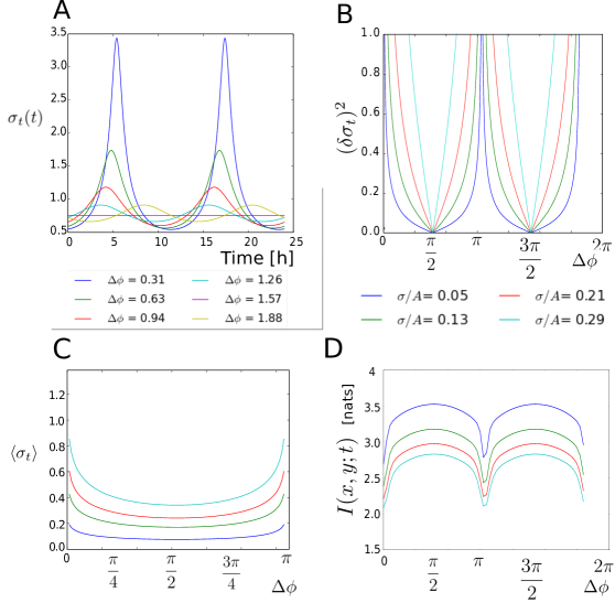
Figure 2: Estimating time via $N=2$ protein oscillations, which have the same relative noise strength $\widetilde{\sigma}_{x}=\sigma_{x}/A$. Here $A$ is the amplitude of the oscillations and $\sigma_{x}$ is the noise in the oscillations, which is here assumed to be constant in time, and given by the mean of the oscillations, $r$, taken to be the same for both oscillations; there are also no cross correlations. (A) The error in the estimate of time $\sigma_{t}(t)$ as a function of time $t$, for different phase differences $\Delta\phi$ between the two oscillations. Note that for $\Delta\phi=\pi/2$, the error $\sigma_{t}(t)$ is constant in time. (B) The variance $(\delta\sigma_{t})^{2}$ in the estimate of time as a function of $\Delta\phi$, for different relative noise strengths $\widetilde{\sigma}_{x}$. As expected from panel A, $(\delta\sigma_{t})^{2}=0$ for $\Delta\phi=\pi/2$. (C) The mean error $\langle\sigma_{t}\rangle$ as a function of $\Delta\phi$, for different relative noise strengths $\widetilde{\sigma}_{x}$. The error is proportional to $\widetilde{\sigma}_{x}$, in accordance with Eq. 28. Note also that the mean error is minimized at $\Delta\phi=\pi/2$, although the dependence on $\Delta\phi$ near the optimum is weak. (D) The mutual information $I(x,y;t)$ between the two protein oscillations $x(t),y(t)$ and time $t$, for different relative noise strengths $\widetilde{\sigma}_{x}$. The mutual information increases with decreasing $\widetilde{\sigma}_{x}$, and is optimized at $\Delta\phi=\pi/2$. Note also that the dependence of $I(x,y;t)$ on $\Delta\phi$ is stronger than that of $\langle\sigma_{t}\rangle$ (panel C).

II.1 No Cross-correlations

In this section, we consider the scenario in which there are no cross correlations between the noise in the expression of the downstream genes. We first study the case in which the relative noise strength, $\widetilde{\sigma}_{i}\equiv\sigma_{i}/A_{i}=\widetilde{\sigma}_{x}$, is the same for all genes $i$; in this scenario, we use the subscript $x$ to remind ourselves that we are considering the standard deviation in $x$ and not in the estimate of time. We will also first assume that $\sigma_{x}(t)=\sigma_{x}$ is constant in time, depending only on the mean of $x$, i.e $r_{x}$, but not its mean instantaneous level $\bar{x}(t)$. The latter is reasonable when the amplitude of the oscillations is small compared to the mean.

To determine the optimal phase relation that miminizes the average error in telling time, given by Eq. 14, we solve

$$\frac{d\langle\sigma_{t}\rangle}{d\Delta\phi_{i}}=0\;\;\;\;\;\;\;\;\;\;i=1...N,$$ (26)

where $\Delta\phi_{i}=\phi_{i}-\phi_{1}$. Setting the phase of the first oscillation to zero, i.e. $\phi_{1}=0$, we find that the optimal phase relation that minimizes the average error is given by

$$\Delta\phi_{i}=(i-1)\frac{\pi}{N}\;\;\;\;\;\;\;\;\;\;i=1...N.$$ (27)

Clearly, in the optimal system the phases of the downstream oscillations are evenly spaced when $\widetilde{\sigma}_{x}$ is the same for all genes, and $\sigma_{x}$ is constant in time.

The next question is what is the phase relation that minimizes the variance of $\sigma_{t}(t)$ over the oscillation period $T$, i.e. minimizes Eq. 15. In the appendix we show that the solution is also given by Eq. 27. Hence, the phase relation that minimizes the average error on telling time, $\langle\sigma_{t}\rangle$, is also the phase relation that minimizes the variance of $\sigma_{t}(t)$. Thus, in the optimal system, the phases are evenly spaced; this not only minimizes the average error in telling time, but it also yields the same accuracy for all times $t$. Moreover, for this optimal system, the average error, obtained from Eq. 12, is given by

$$\langle\sigma_{t}\rangle=\frac{\widetilde{\sigma}_{x}T}{2\pi}\sqrt{\frac{2}{N}}$$ (28)

This shows that the average error is proportional to the relative noise strength $\widetilde{\sigma}_{x}=\sigma_{x}/A$ and inversely proportional to the square root of the number of readout genes, $N$.

These results are illustrated in Figs. 2A-C, for $N=2$. Panel A shows $\sigma_{t}(t)$ as a function of $t$, for different phase relations $\Delta\phi\equiv\phi_{2}-\phi_{1}$. It is seen that, in general, $\sigma_{t}(t)$, depends on $t$. However, when $\Delta\phi=\pi/2$, then $\sigma_{t}(t)$ is independent of $t$. Panel B shows that for this phase relation, the variance $(\delta\sigma_{t})^{2}$ is indeed zero, while panel C shows that in this case also the average error is minimal, in accordance with the theoretical analysis.

Lastly, Fig. 2D shows the mutual information $I(x,y;t)$, obtained numerically, as a function of the phase shift, for different noise levels. As expected, the mutual information increases as the relative noise strength $\widetilde{\sigma}_{x}$ decreases. Moreover, the phase relation that minimizes the average error, $\langle\sigma_{t}\rangle$, is also the phase relation that maximizes the mutual information.

When the noise amplitude $\sigma_{x}$ depends on the mean instantaneous copy number $\bar{x}(t)$ (rather than its mean averaged over the oscillation period), the noise in the output $\sigma_{x}(t)$ varies in time. We will assume that $\sigma_{x}(t)\simeq\sqrt{\bar{x}(t)}$, and consider as above the case that the amplitude and the mean of the oscillations are the same for all genes, respectively: $A_{i}=A_{j}=\dots=A$ and $r_{i}=r_{j}=\dots=r_{x}$. Our analysis described in the appendix reveals that the optimal phase relation that maximizes the mutual information and minimizes both the variance $(\delta\sigma_{t})^{2}$ and the mean $\langle\sigma_{t}\rangle$ of the error, is again given by Eq. 27. However, the minimal variance, obtained for the optimal phase relation, only reduces to zero in the limit that $r\to\infty$; in this limit, the noise $\sigma_{x}(t)$ becomes constant in time and we recover the case discussed above. Interestingly, the average error $\langle\sigma_{t}\rangle$ is larger than that in the case of constant relative noise strength, even when the average relative noise strength is the same.

When $N=2$ yet the relative noise strength is not the same for both genes, $\widetilde{\sigma}_{x}\neq\widetilde{\sigma}_{y}$, the optimal phase shift that minimizes the error and maximizes the mutual information is again $\Delta\phi_{xy}=\pi/2$; indeed, this result, for $N=2$, does not depend on whether $\widetilde{\sigma}$ is the same for both genes. Also the variance $(\delta\sigma_{t})^{2}$ is zero for this optimal phase shift, as before.

These results change markedly when the relative noise strength is not the same for all genes and $N>2$. Then the optimal phase shift depends in a non-trivial manner on $\{\widetilde{\sigma}_{i}\}$. The principle is that the oscillations that contain more information about time because they are less noisy, should be spaced further apart. More specifically, the spacing between them should be closer to that which maximizes the mutual information between them and time. This principle is illustrated in Fig. 3A-B for three genes, where $\widetilde{\sigma}_{x}=\widetilde{\sigma}_{y}\equiv\widetilde{\sigma}_{x,y}<\widetilde{\sigma}_{z}$. Clearly, the oscillations of proteins X and Y contain more information about time than the oscillation of protein Z. As a consequence, the phase difference between $x(t)$ and $y(t)$, $\Delta\phi_{xy}=\phi_{y}-\phi_{x}$, is more important in accurately telling time than that between the two other pairs of oscillations. The phase difference $\Delta\phi_{xy}$ is therefore closer to $\pi/2$, the phase difference that maximizes $I(x,y;t)$, than those of the other pairs of genes. Indeed, the extent to which $\Delta\phi_{xy}$ approaches $\pi/2$ depends on $\widetilde{\sigma}_{x,y}/\widetilde{\sigma}_{z}$, as Fig. 3B shows: when $\widetilde{\sigma}_{x,y}=\widetilde{\sigma}_{z}$, all oscillations are equally informative and hence the oscillations are evenly spaced, yielding $\Delta\phi_{xy}=\Delta\phi_{yz}=\Delta\phi_{zx}=\pi/3$. In contrast, when $\widetilde{\sigma}_{x,y}/\widetilde{\sigma}_{z}=0$, $\Delta\phi_{xy}=\pi/2$, the same result that would have been obtained if these two genes were the only ones present. In this limit, $\widetilde{\sigma}_{z}$ is infinite, and $z$ carries no information on time, making its phase irrelevant.

Fig. 3C gives the mean error $\langle\sigma_{t}\rangle$ and Fig. 3D the mutual information $I(x,y,z;t)$ for the optimal phase relation shown in panel B, as a function of $\widetilde{\sigma}_{xy}/\widetilde{\sigma}_{z}$. Here, in varying $\widetilde{\sigma}_{xy}/\widetilde{\sigma}_{z}$, $\widetilde{\sigma}_{xy}$ is kept constant while $\widetilde{\sigma}_{z}$ is varied between $\widetilde{\sigma}_{xy}$ and infinity. These panels thus show the gain in employing an additional readout protein in accurately telling time, as a function of its noise level. The results interpolate between those for $N=2$ equally informative genes when $\widetilde{\sigma}_{xy}/\widetilde{\sigma}_{z}=0$, and those for $N=3$ equally informative genes when $\widetilde{\sigma}_{xy}/\widetilde{\sigma}_{z}=1$.

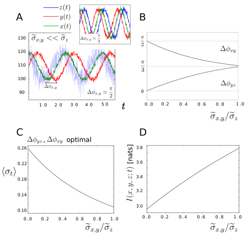
Figure 3: Estimating time via $N=3$ protein oscillations, where the relative noise strength $\widetilde{\sigma}_{i}\equiv\sigma_{i}/A_{i}$ of two oscillations is the same, $\widetilde{\sigma}_{x}=\widetilde{\sigma}_{y}\equiv\widetilde{\sigma}_{x,y}$, and different from that of the third oscillation, $\widetilde{\sigma}_{z}$. The noise $\sigma_{i}$ is assumed to be constant in time, and there are no cross correlations in the noise. (A) Sketch of the set up, with two reliable oscillations $x(t)$ and $y(t)$ and a third, more noisy oscillation $z(t)$. (B) The optimal phase relation that maximizes the mutual information $I(x,y,z;t)$ and minimizes the mean error $\langle\sigma_{t}\rangle$, as a function of $\widetilde{\sigma}_{x,y}/\widetilde{\sigma}_{z}$; here $\widetilde{\sigma}_{x,y}$ is kept constant while $\widetilde{\sigma}_{z}$ is varied. When $\widetilde{\sigma}_{x,y}/\widetilde{\sigma}_{z}=0$, the third gene $z(t)$ carries no information, and the optimal phase difference $\Delta\phi_{xy}=\phi_{y}-\phi_{x}$ between the oscillations of $x$ and $y$ is $\Delta\phi_{xy}=\pi/2$, the result for $N=2$ oscillations; in this limit, the phase of $z$ is irrelevant. As $\widetilde{\sigma}_{x,y}/\widetilde{\sigma}_{z}$ increases, the third oscillation $z(t)$ becomes more important. The phase difference $\Delta\phi_{xy}$ between $x(t)$ and $y(t)$ decreases, while the phase difference $\Delta\phi_{yz}$ between $y(t)$ and $z(t)$ increases. When $\widetilde{\sigma}_{x,y}/\widetilde{\sigma}_{z}=1$, all genes are equally informative and $\Delta\phi_{xy}=\Delta\phi_{yz}=\Delta\phi_{zx}=\pi/3$. (C) The mean error $\langle\sigma_{t}\rangle$ as a function $\widetilde{\sigma}_{x,y}/\widetilde{\sigma}_{z}$. It decreases as the third gene becomes more informative. (D) The mutual $I(x,y,z;t)$ increases with $\widetilde{\sigma}_{x,y}/\widetilde{\sigma}_{z}$.

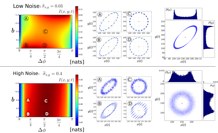
Figure 4: The importance of cross correlations between the fluctuations in the oscillations of the readout proteins, illustrated here for $N=2$ readout proteins. The top row shows results for the scenario in which the relative noise strength $\widetilde{\sigma}_{i}\equiv\sigma_{i}/A_{i}$ is low, while the bottom panel displays the results for when it is large. In all cases, the relative noise strength of the two oscillations is taken to be the same, $\widetilde{\sigma}_{x}=\widetilde{\sigma}_{y}=\widetilde{\sigma}_{x,y}$. The panels in the left column show a heat map of the mutual information $I(x,y;t)$ as a function of the phase difference $\Delta\phi=\phi_{y}-\phi_{x}$ between the two oscillations, and the correlation coefficient $b$. Due to the symmetry of the problem the mutual information is symmetric: $I(x,y;t)_{\Delta\phi,b}=I(x,y;t)_{\pi-\Delta\phi,-b}$. The top-left panel shows that when the relative noise strength is low, the mutual information is maximized for $|b|\to 1$ and $\Delta\phi\neq\pi/2$. Cross correlations thus change the optimal phase difference, and more, importantly, they can enhance the mutual information. However, when the relative noise is large, the cross correlations become less important and the optimal phase difference approaches $\Delta\phi=\pi/2$ (bottom left panel). The middle panels elucidate how cross correlations can affect the mutual information. Shown are, for different points in the heat map on the left, the average trajectory that ${x}(t)$ and $y(t)$ trace out during a 24 hr period (green solid line), with superimposed, for different times of the day, scatter points of $x(t)$ and $y(t)$, originating from gene expression noise. The main axis of the contour $\bar{x}(t),\bar{y}(t)$ is determined by the phase difference $\Delta\phi$, while the main axis of the noise (scatter points) is determined by the correlation coefficient $b$. There are moments of the day where cross correlations cause the distributions $P(x,y|t)$ of neighboring times $t$ to overlap less, thus increasing mutual information, but also moments where they increase the overlap, decreasing the mutual information. The net benefit depends on how these contributions are weighted. The system spends more time near the extrema of $\bar{x}(t),\bar{y}(t)$, as illustrated in the right panels. Consequently, when $\Delta\phi<\pi/2$, positive correlations $b>0$ enhance the mutual information, especially when the relative noise strength $\widetilde{\sigma}_{x}$ is low (point B top row). At higher noise (bottom row), cross correlations are less effective in reducing the overlap in $P(x,y|t)$ and the phase difference $\Delta\phi$ becomes the dominant control parameter.

II.2 The importance of cross-correlations

So far we have assumed that the noise in the expression of the downstream genes is uncorrelated. However, in general, we expect their noise to be correlated. Direct or indirect regulatory interactions between the genes can lead to correlations or anti-correlations in the fluctuations of the protein concentrations Walczak:2010cv . And also noise in the input signal can lead to correlated gene expression. In fact, the extrinsic contribution to the noise in gene expression is often larger than the intrinsic one Taniguchi:2010cb , which can induce pronounced correlations between the expression of the downstream genes. Intuitively, we may think that if we need to infer an input variable $t$ from two output variables $x$ and $y$, then cross-correlations between $x$ and $y$ reduce the accuracy of the estimate—asking two persons $x$ and $y$ a question about $t$ seems to give more information when $x$ and $y$ give independent answers. However, this intuition is not always correct, as will become clear. Indeed, in this section we study how correlations between the expression of downstream genes affect the precision by which cells can tell time.

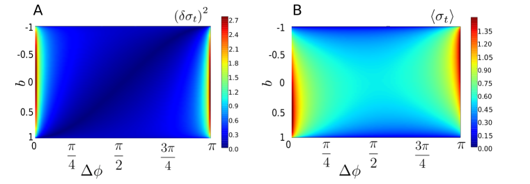
Figure 5: Importance of cross correlations in reducing the error in estimating the time, as estimated from $N=2$ protein oscillations. Heat maps of the the variance in the error $(\delta\sigma_{t})^{2}$ (A) and the mean error $\langle\sigma_{t}\rangle$ (B), as a function of the phase difference $\Delta\phi$ between the two oscillations and the correlation coefficient $b$ of the fluctuations in the oscillations. The relative noise strength $\widetilde{\sigma}_{x}$ is the same for both oscillations, and equal to that of the low-noise scenario in Fig. 4, $\widetilde{\sigma}_{x}=0.03$. It is seen that cross correlations can reduce the mean error. Comparing against the top-left panel of Fig. 4 shows, however, that the positions of the optima are different for the two quantities, the mean error $\langle\sigma_{t}\rangle$ and the mutual information $I(x,y;t)$ , respectively. This is because the quantities $\sigma_{t}(t)$ (Eq. 14) and $H(t|x,y)$ (Eq. 30) are averaged over different distributions, the uniform distribution $P(t)$ and the non-uniform distribution $P(x,y)$, respectively.

In order to dissect the effect of cross-correlations, we study two downstream genes, $N=2$, and take both the amplitudes of their oscillations and their expression noise to be equal: $A_{x}=A_{y}=A$, $\sigma_{x}=\sigma_{y}=\sigma_{x,y}$, respectively. Using the latter, we can renormalize the covariance matrix Eq. 18:

$${\bf C}=\left(\begin{array}[]{cc}\sigma_{x}&\mbox{cov}_{xy}\\ \mbox{cov}_{xy}&\sigma_{y}\\ \end{array}\right)=\sigma_{x,y}\left(\begin{array}[]{cc}1&b\\ b&1\\ \end{array}\right),$$ (29)

where $b$ is the correlation coefficient, denoting the cross-correlation strength: $b=1$ implies that the noise in the expression of X and Y is fully correlated, while $b=-1$ implies full anti-correlation. We computed numerically how $I(x,y;t)$, $\langle\sigma_{t}\rangle_{t}$ and $(\delta t)^{2}$ depend on the phase shift $\Delta\phi=\phi_{y}-\phi_{x}$, the relative noise strength $\widetilde{\sigma}_{x,y}=\sigma_{x,y}/A$, and the correlation coeffient $b$.

Fig. 4 shows the mutual information $I(x,y;t)$ as a function of $\Delta\phi$ and $b$, both for low noise, with $\widetilde{\sigma}_{x,y}=0.03$ (panels top row), and high noise, with $\widetilde{\sigma}_{x,y}=0.4$ (panels bottom row). The following points are worthy of note. First, as expected, $I(x,y;t)$ is symmetric with respect to $\Delta\phi$ and $b$: $I(x,y;t)_{\Delta\phi,b}=I(x,y;t)_{2\pi-\Delta\phi,-b}$. Secondly, depending on the phase shift $\Delta\phi$, correlations ($b>0$) or anti-correlations ($b<0$) can enhance the mutual information, especially when the relative noise strength $\widetilde{\sigma}_{x,y}$ is low (top panel). Concomittantly, the optimal phase shift $\Delta\phi$ that maximizes the mutual information depends on the cross correlation $b$. At low noise, the mutual information is maximized either at $0<\Delta\phi^{*}<\pi/2$ and $b\approx 1$ or at $\pi-\Delta\phi^{*}$ and $b\approx-1$. At high noise, cross correlations no longers help to improve the mutual information (bottom panel). Moreover, the optimal phase shift is at $\Delta\phi^{*}\approx\pi/2$. We now discuss the origin of these observations.

To elucidate these observations, we start from the definition of the mutual information (see Eq. 25):

$$I(x,y;t)=H(t)-\langle H(t|x,y)\rangle_{x,y}$$ (30)

Here, $H(t)$ is the entropy of the input signal, with $P(t)=1/T$. It does not depend on the design of the downstream readout system. In contrast, the second term, $\langle H(t|x,y)\rangle_{x,y}$, does depend on it. We now describe how changing $\Delta\phi$ and $b$ affects this term, using the scatter plots and distributions in the middle and right column of Fig. 4.

The middle panel shows for different combinations of $b$ and $\Delta\phi$, corresponding to the points A,B,C,D in the heat map of $I(x,y;t)$ (left panel), scatter plots of $x(t)$ and $y(t)$. The overall shape of each scatter plot is determined by the phase difference $\Delta\phi$. When $\Delta\phi=\pi/2$ (points C and D), the average expression levels $\bar{x}(t)$ and $\bar{y}(t)$ trace out a circle in state space during a 24 hr period, while when $\Delta\phi=\pi/4$ (points A and B), they carve out an ellipsoidal path; these mean paths are indicated by thin solid green lines in the scatter plots. For each moment of the day, however, $x$ and $y$ will exhibit a distribution of expression levels, due to gene expression noise. This distribution $P(x,y|t)$ is shown as scatter points $(x,y)$ for different yet evenly spaced times $t$ in the respective subpanels. When the main axis of $P(x,y|t)$ is perpendicular to the local tangent of the mean path of $\bar{x}(t),\bar{y}(t)$, then cross correlations reduce $H(t|x,y)$ for that period of the day: the cross correlations cause the distributions $P(x,y|t)$ for neighboring times $t$ to overlap less, meaning that a given point $(x,y)$ maps more uniquely onto a given time $t$. This tends to increase the mutual information. However, as the middle panel illustrates, there are not only moments of the day when the main axis of the scatter points is perpendicular to the local tangent of the mean path, but also times when they are parallel, in which case cross correlations are detrimental. Whether the net result of cross correlations is beneficial, depends on how these different contributions are weighted: $H(t|x,y)$ has to be averaged over $P(x,y)$, see Eq. 30. When $\Delta\phi=\pi/2$, the mean path $\bar{x}(t),\bar{y}(t)$ is circular, yet the net effect of correlations on the mutual information is already positive (left panel), and independent of the sign of $b$. For $\Delta\phi\neq\pi/2$, the effect depends on the sign of $b$. Moreover, the effect is also stronger, because the system spends more time near the extrema of $\bar{x}(t),\bar{y}(t)$, as the right panel illustrates. When $\Delta\phi<\pi/2$, positive correlations in the expression of $x$ and $y$ ($b>0$) cause the main axis of $P(x,y|t)$ to be perpendicular to the local tangent of $\bar{x}(t),\bar{y}(t)$ near the extrema (point B), thus increasing the mutual information, while anti-correlations ($b<0$) cause $P(x,y|t)$ to be parallel to it (point A), decreasing the mutual information. For $\Delta\phi\rightarrow\Delta\phi-\pi/2$ precisely the oppositive behavior is observed, because the mean path of $\bar{x}(t),\bar{y}(t)$ (the ellipse) is flipped vertically. The principal observation is thus that cross-correlations can enhance the mutual information by allowing for a less overlapping tiling of state space, and hence a less redundant mapping between the input $t$ and output $(x,y)$.

For higher noise (panels in lower row of Fig. 4), each $P(x,y|t)$ becomes wider, which means that the benefit of introducing cross correlations in reducing the overlap between different $P(x,y|t)$ (corresponding to different times $t$), decreases. Indeed, at higher noise, the mutual information depends much more weakly on the magnitude of the cross correlations (left panel bottom row). The key control parameter is now the phase shift $\Delta\phi$. For $\Delta\phi=\pi/2$, the distributions $P(x,y|t)$ are most evenly spaced. This minimizes the overlap between them and maximizes the mutual information.

Fig. 5 shows the the variance in the error, $(\delta t)^{2}$, and the average error in telling time, $\langle\sigma_{t}\rangle$, as a function of $\Delta\phi$ and $b$, for $\widetilde{\sigma}=0.03$ (as in the top row of Fig. 4). It is seen that increasing correlations $|b|$ can reduce the average error. Surprisingly, however, for $|b|\approx 1$, the average error $\langle\sigma_{t}\rangle$ is minimized at a phase shift that does not maximize the mutual information, as a comparison with Fig. 4 shows. This is because of how the respective quantities are averaged. The quantity $\sigma_{t}(t)$ is averaged over $P(t)$, which is uniform in time, while $H(t|x,y)$ is averaged over $P(x,y)$, which gives more weight to those points $(x,y)$ that are more probable.

III Discussion

Cells can increase the transmission of temporal information by increasing the number of oscillatory signals $N$ used to infer the time. In the analysis presented here, it is assumed that the system is linear and obeys Gaussian statistics, yet, especially at high noise, it might be beneficial to use non-linear input-output relations to enhance information transmission DeRonde:2014fq . Nonetheless, our linear model highlights that this is a rich problem. The precision of telling time depends on the relative noise $\widetilde{\sigma}_{i}=\sigma_{i}/A_{i}$ of the oscillatory signals, their phase shift, and the cross-correlations between them. When the relative noise $\widetilde{\sigma}_{i}$ is the same for all genes, the optimal phase relation that maximizes the mutual information and minimizes the error is one in which the phases are spaced evenly. Under this condition, the error in telling time is also uniform in time, provided that the noise $\sigma_{i}(t)$ is constant in time, which, to a good approximation, is the case when the amplitude of the oscillations is large compared to the mean. This is akin to what has been observed for the fruitfly Drosophila, where the expression pattern of the gap genes allows the nuclei to specificy their position with nearly uniform precision along the anterior-posterior axis Dubuis2013 . When the relative noise amplitudes $\widetilde{\sigma}_{i}$ are not the same for all signals, then the design principle for maximizing information transmission is that the oscillatory signals which are more reliable, should be spaced more evenly. Lastly, we have addressed the role of cross correlations between the fluctuations in the oscillatory signals. When the relative noise is large, cross-correlations do not significantly affect information transmission. However, the situation changes markedly in the low-noise regime. In this regime, cross-correlations change the optimal phase shift that maximizes information transmission. More strikingly, they can increase the mutual information. At low noise, cross correlations can thus reduce the error in telling time and enhance the transmission of temporal information. This phenomenon is similar to what has been observed for neural networks Tkacik2010 and spatial gene expression patterns during embryonic development, where cross-regulatory interactions between genes can enhance the precision by which cells or nuclei determine their spatial position within the developing embryo Tkacik:2009ta ; Walczak:2010cv ; Dubuis2013 . In all these cases the principle is that cross-correlations make it possible to tile the output space more efficiently, thus allowing for a less redundant input-output mapping. This is particularly important when the noise is low, and noise averaging is not important, but efficient tiling of state space is Tkacik:2009ta ; Walczak:2010cv .

The question that remains is how cells can optimize the relative noise of the oscillatory signals, their phase difference and their cross-correlations. Fluctuations in the input will lead to correlated fluctuations in the oscillations of the output components. Our analysis shows that these correlations can be beneficial. Moreover, they can be tailored via cross-regulatory interactions between the target genes downstream, as in the gap-gene system of Drosophila Tkacik:2009ta ; Walczak:2010cv ; Dubuis2013 . Here, it should be realized that in our analysis we assume that the noise is uncorrelated from the signal; indeed, the mean trajectory $(\bar{x}(t),\bar{y}(t))$ does not depend on the noise. Cross-regulatory interactions will, however, not only affect the noise and hence $P(x,y|t)$, but also the mean trajectory $(\bar{x}(t),\bar{y}(t))$. This will not change the principle that noise correlations can enhance the input-ouput mapping, but it will influence the magnitude of the effect. On the other hand, extrinsic noise sources such as the availability of ribosomes, may lead to correlated fluctuations in the expression of $x(t)$ and $y(t)$, while leaving their mean unchanged, as assumed here. Experiments will have to tell whether cells use noise correlations to enhance the precision of telling time. The cyanobacterium S. elongatus is arguably the best model system to test these ideas. It will certainly be of interest to investigate whether S. elongatus exploits cross-regulatory interactions between the genes downstream from RpaA to enhance its information on time.

The relative noise of the oscillations depends on the noise $\sigma_{i}$ and the amplitude $A_{i}$ of the oscillations. The contribution from the intrinsic noise is expected to scale with the copy number $X$ as $\sigma_{{\rm in},i}\sim\sqrt{X_{i}}$, which, if the amplitude is small compared to the mean $r_{i}$, means that $\sigma_{{\rm in},i}\sim\sqrt{r_{i}}$. The relative intrinsic noise thus goes as $\widetilde{\sigma}_{{\rm in},i}\sim\sqrt{r_{i}}/A_{i}$. For the model presented in section I.1, it is given by

$$\widetilde{\sigma}_{{\rm in},i} \simeq \sqrt{r_{i}}/A_{i}$$ (31)

$$= \sqrt{r_{s}/f_{i}}\sqrt{(\mu_{i}^{2}+\omega^{2})/\mu_{i}}/A_{s}.$$ (32)

Clearly, the relative noise strength $\widetilde{\sigma}_{{\rm in},i}$ decreases with $A_{s}$: the amplitude of the oscillations of the readout is proportional to that of the input. The relative noise strength decreases with the square root of $f_{i}$, because the gain $f_{i}$ increases not only the amplitude of the output oscillations, $A_{i}\propto f_{i}$, but also their mean $r_{i}$ and thereby the noise, $\sigma_{{\rm in},i}\propto\sqrt{r_{i}}\propto\sqrt{f_{i}}$. It increases with the mean $r_{s}$ of the input oscillations, because that increases the mean $r_{i}$ of the output oscillations and thereby the noise $\sigma_{{\rm in},i}$, but not their amplitude, thus decreasing the relative noise strength $\sigma_{{\rm in},i}/A_{i}$. Finally, there exists an optimal protein decay rate $\mu_{\rm opt}=\omega$ that minimizes the relative noise strength and hence maximizes information transmission. This optimum arises from a trade-off between the amplitude of the signal and the intrinsic noise: for $\mu\gg\omega$, increasing $\mu$ reduces the gain and hence the amplitude $A_{i}$ as $A_{i}\propto 1/\mu$ (Eq. 4) while the noise decreases more slowly as $\sqrt{r_{i}}\propto 1/\sqrt{\mu}$, thus increasing the relative noise strength $\widetilde{\sigma}_{{\rm in},i}$; in contrast, for $\mu\ll\omega$, the amplitude $A_{i}$ becomes independent of $\mu_{i}$ (Eq. 4) while the noise continues to rise as $\mu_{i}$ decreases, thus again increasing the relative noise strength.

For the transmission of a fluctuating input signal, a similar trade-off between the gain and the intrinsic noise has been observed in tostevin10 and a related trade-off between mechanistic error arising from the intrinsic noise and dynamical error due to the distortion of the input signal has been described in Bowsher:2013jh . A seemingly similar but distinct trade-off, also leading to an optimal decay rate of the output component, has been reported in Becker2015 : in that study the optimal decay rate arises from the trade-off between tracking the input signal and integrating out the noise in the input signal. Indeed, in our discussion here, we have so far ignored the extrinsic noise in the input signal, and only focused on the intrinsic noise. However, the decay rate $\mu_{i}$ does not only affect the output copy number and thereby the intrinsic noise, it also determines how effectively fluctuations in the input signal can be integrated out. More specifically, if the noise in the input $\xi_{s}$ (Eq. 3) is independent from the input signal, has amplitude $\sigma_{s}$ and decays exponentially with correlation time $\lambda$, then we expect that the extrinsic contribution to the output noise is $\sigma^{2}_{{\rm ex},i}=g_{i}^{2}\mu_{i}/(\mu_{i}+\lambda)\sigma^{2}_{s}$ paulsson2003 ; tanase-nicola06 , where the gain is $g_{i}=f_{i}/\mu_{i}$. Hence, the relative extrinsic noise is

$$\sigma_{{\rm ex},i}/A_{i}=1/\mu_{i}\sqrt{(\mu_{i}^{2}+\omega^{2})\mu_{i}/(\mu_{i}+\lambda)}\sigma_{s}.$$ (33)

We first note that, in contrast to the relative contribution of the intrinsic noise, $\sigma_{{\rm in,i}}/A_{i}$, the relative extrinsic noise does not depend on $f_{i}$: increasing $f_{i}$ raises not only the amplitude of the signal, but also that of the noise; increasing $f_{i}$ is thus only useful in raising the signal above the intrinsic noise. Secondly, for $\mu_{i}\gg\omega,\lambda$, $\sigma_{{\rm ex},i}/A_{i}\simeq\sigma_{s}$, because the time integration factor $\mu_{i}/(\mu_{i}+\lambda)$ becomes constant (independent of $\mu_{i}$), and both the amplitude of the signal, $A_{i}$, and the amplification of the input noise, $g_{i}$ decrease as $\mu_{i}^{-1}$. For $\mu_{i}\ll\omega,\lambda$, $\sigma_{{\rm ex},i}/A_{i}\simeq\omega\sigma_{s}/\sqrt{\mu_{i}\lambda}$, because the amplitude $A_{i}$ becomes independent of $\mu_{i}$, while the extrinsic contribution $\sigma_{{\rm ex},i}$ rises with decreasing $\mu_{i}$ as $1/\sqrt{\mu_{i}}$. In fact, the relative strength of the extrinsic noise $\sigma^{2}_{{\rm ex},}/A_{i}$ has a minimum at $\mu_{\rm ex}^{\rm opt}=(\omega^{2}/\lambda)(1+\sqrt{1+(\lambda/\omega)^{2}})$. We thus conclude that both the relative strength of the intrinsic and extrinsic noise exhibit a minimum as function of $\mu_{i}$, meaning that there is an optimal protein lifetime that maximizes information transmission.

Lastly, how could cells optimize the phase relation between the oscillations of the readout proteins? In the simple model of I.1 there is only one control variable, namely the protein degradation rate (Eq. 5). Clearly, it is not possible, in general, to simultaneously set the decay rate such that the relative noise strength is minimized, as described above, and the phase difference is optimized. However, the simple model of I.1 ignores that gene expression is, in fact, a multi-step process leading to a delay, and it is possible that nature has tuned this delay so as to optimize the phase relation between the output oscillations. In addition, cells could use gene expression cascades to adjust the delay. Whether cells employ these mechanisms to optimize the phase relation is an interesting question for future work.

Appendix A The optimal phase relation in the absence of cross correlations

We would like to compute the phase relation that minimizes the variance of the error, $(\delta\sigma_{t})^{2}$, as given by Eq. 15, in the absence of cross correlations. However, the problem is that Eq. 11 is an expression for $\sigma_{t}^{-2}(t)$, not $\sigma_{t}(t)$. Hence, while it is fairly straightforward to derive the variance of $\sigma_{t}^{-2}$, i.e. $\langle(\sigma_{t}^{-2})^{2}\rangle-\langle\sigma_{t}^{-2}\rangle^{2}$, it is impossible, in general, to derive analytically the variance of the quantity we are interested in, $(\delta\sigma_{t})^{2}=\langle\sigma_{t}^{2}\rangle-\langle\sigma_{t}\rangle^{2}$. However, we know that if the variance of a function $g(t)$ is zero, $\sigma^{2}_{g}=\int_{0}^{T}dtP(t)(g(t)-\langle g(t)\rangle)^{2}=0$, and $g(t)$ is thus a constant (independent of time), that then a) $\langle f(g(t))\rangle=f(\langle g(t)\rangle)$ and b) the variance of $f(t)=f(g(t))$ is zero, $\sigma^{2}_{f}=\langle f^{2}\rangle-\langle f\rangle^{2}=0$. We now apply this logic with the identification $g(t)=\sigma_{t}(t)$ and $f(t)=g^{-2}(t)$. The trick that we thus employ is to establish that the variance which we can compute, $\sigma^{2}_{f}=\langle(\sigma_{t}^{-2})^{2}\rangle-\langle\sigma_{t}^{-2}\rangle^{2}$, is zero. If this is true, then we know that a) the variance of the quantity that we are interested in, $\sigma^{2}_{g}=(\delta\sigma_{t})^{2}$, must be zero as well. Moreover, we then also know that b) $\langle\sigma_{t}\rangle=\sigma_{t}=1/\sqrt{\langle\sigma^{-2}_{t}(t)\rangle}$.

There are two points worthy of note. First, as mentioned, above, when $\sigma^{2}_{f}=\langle(\sigma^{-2}_{t}(t))^{2}\rangle-\langle\sigma^{-2}_{t}(t)\rangle^{2}=0$, then $(\delta\sigma_{t})^{2}=0$. In this case, the phase relation that minimizes $\sigma^{2}_{f}$ is the phase relation that minizes $\delta\sigma^{2}_{t}$ (making it zero indeed). However, when $\sigma^{2}_{f}\neq 0$, then the phase relation that minimizes $\sigma^{2}_{f}$ is not necessarily the phase relation that minimzes $\delta\sigma^{2}_{t}$. Secondly, the phase relation that minimizes $(\delta\sigma_{t})^{2}$, is not necessarily the phase relation that minimizes $\sigma_{t}$, even when $(\delta\sigma_{t})^{2}=0$. We need to check either numerically or, if possible, by analytically minizing $\langle\sigma_{t}\rangle$ whether this is true or not. The same holds for the mutual information: the phase relation that minimizes $(\delta\sigma_{t})^{2}$, is not necessarily the phase relation that maximizes the mutual information.

A.1 The phase relation that minimizes $(\delta\sigma_{t})^{2}$ when the relative noise strengths are the same

As explained above, to obtain the optimal phase relation that makes $(\delta\sigma_{t})^{2}=0$, we aim to find the phase distribution for which:

$$\sigma^{2}_{f}=\langle(\sigma^{-2}_{t}(t))^{2}\rangle-\langle\sigma^{-2}_{t}(t)\rangle^{2}=0.$$ (34)

When the cross correlations are zero, $\sigma^{-2}_{t}(t)$ is given by Eq. 12. The second term in the expression above, $\langle\sigma^{-2}_{t}(t)\rangle^{2}$, is then, for the case that the noise and the ampltidues are the same for all genes, given by

$$\langle\sigma^{-2}_{t}(t)\rangle=\left(\frac{2\pi A}{\sigma_{x}T}\right)^{2}\frac{N}{2}.$$ (35)

The first term in Eq. 34 can be obtained recursively, and is given by

$$\langle(\sigma^{-2}_{t}(t))^{2}\rangle=$$

$$K\left[\frac{N(2N+1)}{8}+\frac{1}{4}\sum_{i<j}^{N}\cos(2(\phi_{i}-\phi_{j}))\right]$$ (36)

where $K$ is a constant, $K=\left(\frac{2\pi A}{\sigma_{x}T}\right)^{4}$. As expected this quantity depends on the phase relation.

Instead of finding the phase relation that makes the difference between the two terms of $\sigma^{2}_{f}$ in Eq. 34 zero, we now want to find the relation that makes the ratio of the two terms unity, which is equivalent, but mathematically more convenient. This yields

$$\frac{2}{N}\sum_{i\leq j}^{N}\cos(2(\phi_{i}-\phi_{j}))=-1.$$ (37)

By solving this as a function of $N$, we can recognize a pattern, which reveals that the optimal phase relation that minimizes $(\delta\sigma_{t})^{2}$ is given by

$$\phi_{i}-\phi_{j}=\frac{\pi}{N}(i-j).$$ (38)

This means that the $i$-th signal has a phase $\Delta\phi_{i}=(i-1)\frac{\pi}{N}$, as found for the phase relation that minimizes $\langle\sigma_{t}\rangle$, given by Eq 27. So in the case where the correlations are zero, the optimal phase shift minimizes both $\langle\sigma_{t}\rangle$ and its variance. Moreover, the mean error $\langle\sigma_{t}\rangle$ can then directly be obtained from Eq. 35.

A.2 The phase relation that minimizes $(\delta\sigma_{t})^{2}$ when the noise $\sigma_{x}$ is not constant in time

We now consider the case that $\sigma_{i}\simeq\sqrt{\bar{x}_{i}(t)}$, which means that $d\sigma_{i}/dt\neq 0$. In order to highlight the role of the time-varying noise, we keep $A_{i}=A_{j}=\dots=A$, $r_{i}=r_{j}=\dots=r$. The variance of $\sigma^{-2}(t)$ is given by:

$$\sigma^{2}_{f} = \langle(\sigma^{-2}_{t}(t))^{2}\rangle-\langle\sigma^{-2}_{t}(t)\rangle^{2}$$ (39)

$$= \left(\frac{A^{3}(2\pi)^{2}}{16T^{2}}\right)^{2}\{N+2N(N+1)r^{2}+$$

$$\sum_{i\leq j}^{N}\left[\cos(\phi_{i}-\phi_{j})+4r^{2}\cos[2(\phi_{i}-\phi_{j})\right]+$$

$$\left.4r^{2}\cos(\phi_{i}-\phi_{j})\right]\}-\left(\frac{NA^{3}r(2\pi)^{2}}{2T^{2}}\right)^{2}$$

We note that this expression, in contrast to that for the case in which $\sigma_{i}$ is constant in time, depends on the mean expression level of $x$, $r$. We find numerically that the phase relation that minimizes $\sigma^{2}_{f}$ is the same as that for the scenario in which $\sigma_{i}$ is constant in time, Eq. 38. However, $\sigma^{2}_{f}$ and hence $(\delta\sigma_{t})^{2}$ are only zero, when $r\to\infty$. We also find numerically that the phase relation that minimizes $\sigma^{2}_{f}$ equals the phase relation that minimizes the mean error $\langle\sigma_{t}\rangle$ and maximizes the mutual information.

A.3 The phase relation that minimizes $(\delta\sigma_{t})^{2}$ when the relative noise strengths are not the same

To assess the importance of differences in the relative noise strength, we will assume again that $\sigma_{i}(t)=\sigma_{i}$ is constant in time. Defining the relative noise amplitude $\widetilde{A}_{i}\equiv\widetilde{\sigma}_{i}^{-1}\equiv A_{i}/\sigma_{i}$, the variance of $\sigma^{-2}(t)$ is given by:

$$\sigma^{2}_{f}=\langle(\sigma^{-2}_{t}(t))^{2}\rangle-\langle\sigma^{-2}_{t}(t)\rangle^{2}$$

$$=\frac{1}{8}\left(\frac{2\pi}{T}\right)^{4}\left[\sum_{i=1}^{N}3\widetilde{A}_{i}^{2}+\sum_{i\leq j}^{N}\left(\left[4+2\cos[2(\phi_{i}-\phi_{j})]\widetilde{A}_{i}\widetilde{A}_{j}\right]\right)\right]$$

$$-\left(\frac{1}{2}\left(\frac{2\pi}{T}\right)^{2}\sum_{i=1}^{N}\widetilde{A}_{i}\right)^{2}$$ (40)

It can be verified that this reduces to Eq. 34 when $\sigma_{i}/A_{i}$ is the same for all genes. Following the logic applied for that scenario, we find that the optimal phase relation that makes $\sigma^{2}_{f}=0$ is given by

$$\sum_{i\leq j}^{N}\cos\left[2(\phi_{i}-\phi_{j})\widetilde{A}_{i}\widetilde{A}_{j}\right]\widetilde{A}_{i}^{2}\widetilde{A}_{j}=$$

$$\sum_{i,j=1}^{N}\widetilde{A}_{i}\widetilde{A}_{j}-\frac{1}{2}\sum_{i=1}^{N}3\widetilde{A}_{i}^{2}-2\sum_{i\leq j}^{N}\widetilde{A}_{i}\widetilde{A}_{j}$$ (41)

This expression reduces to Eq. 37 when $\sigma_{i}/A_{i}$ is the same for all genes. It can be verified numerically that the phase relation that makes $\sigma^{2}_{f}$ and hence $(\delta\sigma_{t})^{2}$ zero, is also the phase relation that minimizes the mean error $\langle\sigma_{t}\rangle$ and maximizes the mutual information.

- [1] Carl Hirschie Johnson, Martin Egli, and Phoebe L Stewart. Structural insights into a circadian oscillator. Science, 322(5902):697–701, October 2008.
- [2] C Liu, D R Weaver, S H Strogatz, and S M Reppert. Cellular construction of a circadian clock: period determination in the suprachiasmatic nuclei. Cell, 91(6):855–860, 1997.
- [3] S Yamaguchi. Synchronization of Cellular Clocks in the Suprachiasmatic Nucleus. Science, 302(5649):1408–1412, November 2003.
- [4] I Mihalcescu, W H Hsing, and S Leibler. Resilient circadian oscillator revealed in individual cyanobacteria. Nature, 430(6995):81–85, 2004.
- [5] David Zwicker, David K Lubensky, and Pieter Rein ten Wolde. Robust circadian clocks from coupled protein-modification and transcription-translation cycles. Supporting info. Proceedings of the National Academy of Sciences of the United States of America, 107(52):22540–5, December 2010.
- [6] Joris Paijmans, Mark Bosman, Pieter Rein Ten Wolde, and David K Lubensky. Discrete gene replication events drive coupling between the cell cycle and circadian clocks. Submitted, 2015.
- [7] Andrew Mugler, Aleksandra Walczak, and Chris Wiggins. Information-Optimal Transcriptional Response to Oscillatory Driving. Physical Review Letters, 105(5):058101, July 2010.
- [8] Hakuto Kageyama, Takao Kondo, and Hideo Iwasaki. Circadian formation of clock protein complexes by KaiA, KaiB, KaiC, and SasA in cyanobacteria. J Biol Chem, 278(4):2388–95, 2003.
- [9] Michael J Rust, Joseph S Markson, William S Lane, Daniel S Fisher, and Erin K O’Shea. Ordered phosphorylation governs oscillation of a three-protein circadian clock. Science, 318(5851):809–12, November 2007.
- [10] Taeko Nishiwaki, Yoshinori Satomi, Yohko Kitayama, Kazuki Terauchi, Reiko Kiyohara, Toshifumi Takao, and Takao Kondo. A sequential program of dual phosphorylation of KaiC as a basis for circadian rhythm in cyanobacteria. EMBO J, 26:4029–4037, 2007.
- [11] Yohko Kitayama, Taeko Nishiwaki, Kazuki Terauchi, and Takao Kondo. Dual KaiC-based oscillations constitute the circadian system of cyanobacteria. Genes Dev, 22:1513–1521, 2008.
- [12] Naoki Takai, Masato Nakajima, Tokitaka Oyama, Ryotaku Kito, Chieko Sugita, Mamoru Sugita, Takao Kondo, and Hideo Iwasaki. A KaiC-associating SasA-RpaA two-component regulatory system as a major circadian timing mediator in cyanobacteria. Proc Natl Acad Sci USA, 103(32):12109–14, 2006.
- [13] Y Taniguchi, M Katayama, R Ito, N Takai, T Kondo, and T Oyama. labA: a novel gene required for negative feedback regulation of the cyanobacterial circadian clock protein KaiC. Gens Dev, 21(1):60–70, January 2007.
- [14] Yasuhito Taniguchi, Naoki Takai, Mitsunori Katayama, Takao Kondo, and Tokitaka Oyama. Three major output pathways from the KaiABC-based oscillator cooperate to generate robust circadian kaiBC expression in cyanobacteria. Proc Natl Acad Sci USA, 107(7):3263–8, 2010.
- [15] Andrian Gutu and Erin K O’Shea. Two antagonistic clock-regulated histidine kinases time the activation of circadian gene expression. Mol Cell, 50(2):288–294, March 2013.
- [16] Joseph S Markson, Joseph R Piechura, Anna M Puszynska, and Erin K O’Shea. Circadian control of global gene expression by the cyanobacterial master regulator RpaA. Cell, 155(6):1396–408, 2013.
- [17] Gasper Tkacik, Jason S Prentice, Vijay Balasubramanian, and Elad Schneidman. Optimal population coding by noisy spiking neurons. Proceedings of the National Academy of Sciences of the United States of America, 107(32):14419–24, August 2010.
- [18] Aleksandra M Walczak, Gašper Tkačik, and William Bialek. Optimizing information flow in small genetic networks. II. Feed-forward interactions. Physical Review E, 81(4):041905, April 2010.
- [19] Julien O Dubuis, Gasper Tkacik, Eric F Wieschaus, Thomas Gregor, and William Bialek. Positional information, in bits. Proceedings of the National Academy of Sciences of the United States of America, 110(41):16301–8, October 2013.
- [20] Johan Paulsson. Summing up the noise in gene networks. Nature, 427:415, 2004.
- [21] Howard C. Berg and Edward M. Purcell. Physics of chemoreception. Biophysical Journal, 20:193, 1977.
- [22] Masahiro Ueda and Tatsuo Shibata. Stochastic signal processing and transduction in chemotactic response of eukaryotic cells. Biophysical Journal, 93(1):11–20, 2007.
- [23] William Bialek and Sima Setayeshgar. Physical limits to biochemical signaling. Proceedings of the National Academy of Sciences USA, 102:10040, 2005.
- [24] Kai Wang, Wouter-Jan Rappel, Rex Kerr, and Herbert Levine. Quantifying noise levels in intercellular signals. Physical Review E, 75:061905, 2007.
- [25] Wouter-Jan Rappel and Herbert Levine. Receptor noise and directional sensing in eukaryotic chemotaxis. Physical Review Letters, 100:228101, 2008.
- [26] Robert G. Endres and Ned S. Wingreen. Maximum likelihood and the single receptor. Physical Review Letters, 103:158101, 2009.
- [27] Bo Hu, Wen Chen, Wouter-Jan Rappel, and Herbert Levine. Physical limits on cellular sensing of spatial gradients. Physical Review Letters, 105:048104, 2010.
- [28] Thierry Mora and Ned S. Wingreen. Limits of sensing temporal concentration changes by single cells. Physical Review Letters, 104:248101, 2010.
- [29] Christopher C Govern and Pieter Rein ten Wolde. Fundamental limits on sensing chemical concentrations with linear biochemical networks. Physical Review Letters, 109(21):218103, 2012.
- [30] Pankaj Mehta and David J Schwab. Energetic costs of cellular computation. Proceedings of the National Academy of Sciences USA, 109(44):17978–17982, 2012.
- [31] Monica Skoge, Yigal Meir, and Ned S Wingreen. Dynamics of Cooperativity in Chemical Sensing among Cell-Surface Receptors. Physical Review Letters, 107(17):178101, October 2011.
- [32] Monica Skoge, Sahin Naqvi, Yigal Meir, and Ned S Wingreen. Chemical sensing by nonequilibrium cooperative receptors. Physical Review Letters, 110(24):248102, June 2013.
- [33] Kazunari Kaizu, Wiet de Ronde, Joris Paijmans, Koichi Takahashi, Filipe Tostevin, and Pieter Rein ten Wolde. The berg-purcell limit revisited. Biophysical journal, 106(4):976–985, 2014.
- [34] Christopher C Govern and Pieter Rein ten Wolde. Optimal resource allocation in cellular sensing systems. Proceedings of the National Academy of Sciences of the United States of America, 111(49):17486–17491, December 2014.
- [35] Christopher C Govern and Pieter Rein ten Wolde. Energy Dissipation and Noise Correlations in Biochemical Sensing. Physical Review Letters, 113(25):258102, December 2014.
- [36] Alex H Lang, Charles K Fisher, Thierry Mora, and Pankaj Mehta. Thermodynamics of Statistical Inference by Cells. Physical Review Letters, 113(14):148103, October 2014.
- [37] Etay Ziv, Ilya Nemenman, and Chris H. WIggins. Optimal signal processing in small stochastic biochemical networks. PloS one, 2(10):e1077, January 2007.
- [38] Filipe Tostevin and Pieter Rein ten Wolde. Mutual Information between Input and Output Trajectories of Biochemical Networks. Physical Review Letters, 102(21):218101, May 2009.
- [39] Pankaj Mehta, Sidhartha Goyal, Tao Long, Bonnie L. Bassler, and Ned S. Wingreen. Information processing and signal integration in bacterial quorum sensing. Molecular systems biology, 5(325):325, January 2009.
- [40] Gašper Tkačik, Aleksandra M Walczak, and William Bialek. Optimizing information flow in small genetic networks. Physical Review E, 80(3 Pt 1):031920, September 2009.
- [41] Filipe Tostevin and Pieter Rein ten Wolde. Mutual information in time-varying biochemical systems. Phys Rev E Stat Nonlin Soft Matter Phys, 81(6 Pt 1):061917, Jun 2010.
- [42] Wiet de Ronde, Filipe Tostevin, and Pieter Rein ten Wolde. Effect of feedback on the fidelity of information transmission of time-varying signals. Physical Review E, 82(3), September 2010.
- [43] Wiet de Ronde, Filipe Tostevin, and Pieter ten Wolde. Multiplexing Biochemical Signals. Physical Review Letters, 107(4):1–4, July 2011.
- [44] R Cheong, A Rhee, C J Wang, I Nemenman, and A Levchenko. Information Transduction Capacity of Noisy Biochemical Signaling Networks. Science, 334(6054):354–358, October 2011.
- [45] W de Ronde, F Tostevin, and P ten Wolde. Feed-forward loops and diamond motifs lead to tunable transmission of information in the frequency domain. Physical Review E, 86(2):021913, August 2012.
- [46] Clive G Bowsher, Margaritis Voliotis, and Peter S Swain. The fidelity of dynamic signaling by noisy biomolecular networks. PLoS Computational Biology, 9(3):e1002965, 2013.
- [47] Jangir Selimkhanov, Brooks Taylor, Jason Yao, Anna Pilko, John Albeck, Alexander Hoffmann, Lev Tsimring, and Roy Wollman. Systems biology. Accurate information transmission through dynamic biochemical signaling networks. Science, 346(6215):1370–1373, December 2014.
- [48] Wiet de Ronde and Pieter Rein ten Wolde. Multiplexing oscillatory biochemical signals. Physical Biology, 11(2):026004, April 2014.
- [49] Thomas R Sokolowski and Gašper Tkačik. Optimizing information flow in small genetic networks. IV. Spatial coupling. Physical Review E, 91(6):062710, June 2015.
- [50] Nils B Becker, Andrew Mugler, and Pieter Rein ten Wolde. Optimal Prediction by Cellular Signaling Networks. Physical Review Letters, Accepted, 2015.
- [51] Gašper Tkačik and Aleksandra M Walczak. Information transmission in genetic regulatory networks: a review. Journal of physics. Condensed matter : an Institute of Physics journal, 23(15):153102, April 2011.
- [52] C. E. Shannon. The mathematical theory of communication. 1963. M.D. computing : computers in medical practice, 14(4):306–17, 1948.
- [53] Y Taniguchi, P J Choi, G W Li, H Chen, M Babu, J Hearn, A Emili, and X S Xie. Quantifying E. coli Proteome and Transcriptome with Single-Molecule Sensitivity in Single Cells. Science, 329(5991):533–538, July 2010.
- [54] Sorin Tănase-Nicola, Patrick B. Warren, and Pieter Rein ten Wolde. Signal detection, modularity, and the correlation between extrinsic and intrinsic noise in biochemical networks. Physical Review Letters, 97(6):068102, August 2006.