CERN-PH-TH/2015-196

Statistical anisotropy from inflationary magnetogenesis

Massimo Giovannini

Theory Department, CERN, 1211 Geneva 23, Switzerland
INFN, Section of Milan-Bicocca, 20126 Milan, Italy

Abstract

Provided the quantum fluctuations are amplified in the presence of a classical gauge field configuration the resulting curvature perturbations exhibit a mild statistical anisotropy which should be sufficiently weak not to conflict with current observational data. The curvature power spectra induced by weakly anisotropic initial states are computed here for the first time when the electric and the magnetic gauge couplings evolve at different rates as it happens, for instance, in the relativistic theory of van der Waals interactions. After recovering the results valid for coincident gauge couplings, the constraints imposed by the isotropy and the homogeneity of the initial states are discussed. The obtained bounds turn out to be more stringent than naively expected and cannot be ignored when discussing the underlying magnetogenesis scenarios.

1 Introduction

Over the last decade the temperature and the polarization anisotropies of the Cosmic Microwave Background (CMB in what follows) have been scrutinized with the aim of finding specific hints signalling a minute breaking of rotational invariance of the power spectrum of curvature perturbations. Both the WMAP [1] and the Planck experiments published dedicated analyses with the aim of estimating the size of this admittedly small effect whose physical consequences could be potentially significant. In particular the seven and nine years WMAP [2, 3, 4] data and the two Planck [5] releases specifically addressed this problem without reaching a conclusive evidence of the possible systematic nature of the effect whose statistical relevance is anyway not yet compelling.

In this situation various authors speculated that the anisotropic correction to the power spectrum of curvature perturbations could be the result of some form of inflationary dynamics leading to a perturbative breaking of rotational invariance (see [6, 7, 8, 9] for a time-ordered but still incomplete list of references). While different models have been examined, a plausible class of scenarios involves the presence of either electric or magnetic fields which must be sufficiently intense to affect the spectra of curvature perturbations but also extremely weak not to spoil the isotropy of the background. This possibility clashes, however, with a relatively well known obstruction represented by the so-called cosmic no-hair conjecture. In conventional inflationary models any finite portion of the universe gradually loses the memory of an initially imposed anisotropy or inhomogeneity so that the universe attains the observed regularity regardless of the initial boundary conditions [10, 11].

The electric or the magnetic energy densities should be roughly constant for most of the inflationary evolution: this is the narrow path to obtain a sufficiently strong effect on the power spectrum and a comparatively negligible impact on the isotropy of the background geometry. In this respect a particularly plausible model is the one based on the coupling of the gauge kinetic term either to the inflaton or to some other spectator field (see, for instance, [12, 13]). This scenario has been recently generalized to a class of models including, as a subcase, the relativistic theory of van der Waals interactions [14]. This framework naturally leads to a different evolution of the electric and magnetic susceptibilities or, equivalently, of the electric and magnetic gauge couplings [15]. In this paper we shall show that the possibility of achieving a substantial anisotropy in the power spectrum can be used to constrain the magnetogenesis scenarios based on the asymmetric evolution of the gauge couplings. The plan of this paper is therefore the following. In section 2 we shall discuss, in a unified manner, the magnetogenesis models based on the coupling of an Abelian gauge field to the inflaton or to some other spectator field. In section 3 we shall derive the evolution of curvature perturbations triggered by the presence of the gauge fields. The anisotropic power spectra and the constraints imposed on the whole scenario will be specifically derived in section 4. Section 5 contains the concluding remarks.

2 Magnetogenesis and statistical anisotropy

2.1 General considerations

We shall now consider a general form of the four-dimensional gauge action written in terms of two symmetric tensors (i.e. ${\mathcal{M}}_{\sigma}^{\rho}$ and ${\mathcal{N}}_{\sigma}^{\rho}$) which may depend on the inflaton field $\varphi$ possibly supplemented by some spectator field $\sigma$:

$$S=-\frac{1}{16\pi}\int d^{4}x\,\sqrt{-G}\biggl{[}\lambda(\varphi,\sigma)Y_{\alpha\beta}Y^{\alpha\beta}+{\mathcal{M}}_{\sigma}^{\rho}(\varphi,\sigma)Y_{\rho\alpha}\,Y^{\sigma\alpha}-{\mathcal{N}}_{\sigma}^{\rho}(\varphi,\sigma)\widetilde{Y}_{\rho\alpha}\,\widetilde{Y}^{\sigma\alpha}\biggr{]},$$ (2.1)

where $G$ denotes the determinant of the four-dimensional metric $G_{\mu\nu}$; in Eq. (2.1) $Y_{\mu\nu}$ and $\widetilde{Y}_{\mu\nu}$ are, respectively, the gauge field strength and its dual. Conformally flat background geometries $G_{\mu\nu}=a^{2}(\tau)\eta_{\mu\nu}$ (where $\tau$ denotes the conformal time coordinate, $a(\tau)$ is the scale factor and $\eta_{\mu\nu}$ the Minkowski metric) will be the main focus of the present analysis but various considerations can also be applied to different backgrounds.

For specific choices of ${\mathcal{M}}_{\sigma}^{\rho}$ and ${\mathcal{N}}_{\sigma}^{\rho}$, Eq. (2.1) reproduces the relativistic theory of van der Waals interactions [14]. The detailed derivation of the equations of motion has been already discussed in Ref. [15] together the relevant symmetries of the system. The evolution equations for the electric and magnetic fields shall then be written as:

$$\vec{\nabla}\times\biggl{(}\sqrt{\Lambda_{B}}\vec{B}\biggr{)}=\partial_{\tau}\biggl{(}\sqrt{\Lambda_{E}}\vec{E}\biggr{)}+4\pi\vec{J},$$ (2.2)

$$\vec{\nabla}\times\biggl{(}\frac{\vec{E}}{\sqrt{\Lambda_{E}}}\biggr{)}+\partial_{\tau}\biggl{(}\frac{\vec{B}}{\sqrt{\Lambda_{B}}}\biggr{)}=0,$$ (2.3)

$$\vec{\nabla}\cdot\biggl{(}\frac{\vec{B}}{\sqrt{\Lambda_{B}}}\biggr{)}=0,\qquad\vec{\nabla}\cdot(\sqrt{\Lambda_{E}}\,\vec{E})=4\pi\rho_{q},$$ (2.4)

where $\vec{J}$ and $\rho_{q}$ are the current and the charge densities. Note, furthermore, that in Eqs. (2.2), (2.3) and (2.4) the electromagnetic fields have been rescaled through the electric and magnetic susceptibilities, i.e. $\vec{B}=a^{2}\,\sqrt{\Lambda_{B}}\,\vec{b}$ and $\vec{E}=a^{2}\,\sqrt{\Lambda_{E}}\,\vec{e}$. Whenever $\vec{J}\to 0$ and $\rho_{q}\to 0$, Eqs. (2.2), (2.3) and (2.4) are invariant under duality transformations generalizing the standard case [16] of coincident gauge couplings.

2.2 Electric and magnetic gauge couplings

Equations (2.2), (2.3) and (2.4) can be expressed in terms of the electric and magnetic susceptibilities defined as $\chi_{E}=\sqrt{\Lambda_{E}}$ and $\chi_{B}=\sqrt{\Lambda_{B}}$; the inverse of the susceptibilities are related to the corresponding gauge couplings as $g_{E}=\sqrt{4\pi/\Lambda_{E}}$ and $g_{B}=\sqrt{4\pi/\Lambda_{B}}$. The time evolution of $g_{E}$ and $g_{B}$ during a quasi-de Sitter stage of expansion amplifies the gauge field fluctuations. In this investigation the curvature perturbations induced by the amplified gauge field fluctuations will be used to constrain the rates of the evolution of the gauge couplings denoted hereunder by $F_{E}$ and $F_{B}$:

$$g_{E}(a)=\overline{g}_{E}\biggl{(}\frac{a}{a_{i}}\biggr{)}^{F_{E}},\qquad g_{B}(a)=\overline{g}_{B}\biggl{(}\frac{a}{a_{i}}\biggr{)}^{F_{B}},\qquad f=\frac{g_{B}^{2}}{g_{E}^{2}}=f_{i}\biggl{(}\frac{a}{a_{i}}\biggr{)}^{2(F_{B}-F_{E})},$$ (2.5)

where $a_{i}$ denotes the scale factor at the onset of the dynamical evolution of the gauge couplings and $f(a)$ measures the mismatch between $g_{E}$ and $g_{B}$. The moment at which the largest wavelength of the curvature perturbations exits the Hubble radius (i.e. $a_{ex}$) may either be ${\mathcal{O}}(a_{i})$ or much larger than $a_{i}$. Even if the present considerations are general, for the specific discussions we shall preferentially consider the case where $a_{i}$ and $a_{ex}$ are of the same order but with $a_{i}<a_{ex}$.

The limit of exactly coincident coupling corresponds to $f(a)=1$ during the whole evolution and, in this case, the standard results apply [12, 13]. Two extreme physical situations can be envisaged: the case when $f\to 1$ at the end of inflation (i.e. $f_{f}={\mathcal{O}}(1)$, the couplings converge towards the end of inflation) and the case when $f\to 1$ at the beginning of inflation (i.e. $f_{i}={\mathcal{O}}(1)$ the couplings converge at the onset of inflation but diverge at the and of inflation). These two limiting situations are purely illustrative and various intermediate possibilities are also physically plausible. Having said this, the constraints derived from the impact of the gauge field fluctuations on the gauge-invariant curvature perturbations will be charted in the $(F_{B},\,F_{E})$ plane and the two benchmark cases of converging couplings (i.e. $f_{f}\to 1$) and of diverging couplings (i.e. $f_{i}\to 1$) will be specifically examined.

If $F_{B}$ and $F_{E}$ are both positive the gauge couplings are initially small and get strong at the end of inflation. Conversely if $F_{B}$ and $F_{E}$ are both negative the gauge couplings may be strong at the beginning of inflation while they get weaker and weaker towards the end. This second situation seems to be the most natural in conventional inflationary models where, initially, the gravitational coupling is potentially very large during the pre-inflationary phase. In the class of models investigated in [15] however, this choice is not mandatory.

2.3 Initial conditions and gauge field fluctuations

The nature of the initial conditions for the evolution of the Abelian gauge fields depends on the unknown features of the protoinflationary phase. For instance we could consider a globally neutral Lorentzian plasma as a possible remnant of a preinflationary stage of expansion and pose the problem of the suitable initial conditions for the evolution of the large-scale electromagnetic inhomogeneities. During the protoinflationary regime, the Weyl invariance of the Ohmic current guarantees that the comoving conductivity is approximately constant. When the electric fields are negligible thanks to the large conductivity of the protoinflationary plasma, the magnetic field is supported by a static solenoidal current obeying, from Eq. (2.2), $\vec{\nabla}\times\biggl{(}\sqrt{\Lambda_{B}}\vec{B}\biggr{)}\simeq 4\pi\vec{J}$. Since the plasma is globally neutral the charge density vanishes in Eq. (2.4). These initial conditions are generally inhomogeneous but they do not induce specific anisotropies. This analysis, in the case of coincident gauge couplings, can be found in [17].

Another example of inhomogenous initial conditions not inducing specific anisotropies are the quantum mechanical initial data. In this case both the current density and the charge density vanish in Eqs. (2.2) and (2.4). Quantum mechanical initial data are justified in the case where, for instance, the duration of inflationary phase is extremely long (i.e. $a_{i}\ll a_{ex}$ in our notations). Purely quantum mechanical initial data have been discussed in a variety of situations [12, 13] in the case of coincident gauge couplings and also in the situation parametrized by Eq. (2.5) [15]. There is a third type of initial data that could be imposed namely the weakly anisotropic initial data: they do not modify the isotropic evolution of the background but may contain either an electric or a magnetic field (or both). We are considering here the situation where the electric and the magnetic fields are sufficiently small not to change the background geometry but large enough to affect the evolution of the curvature inhomogeneities.

In the absence of sources the evolution of the electric and magnetic fields can be separated into a homogeneous part (i.e. $E^{(0)}_{i}(a)$ and $B^{(0)}_{i}(a)$) supplemented by a fully inhomogeneous contribution denoted, in real space, by $E^{(1)}_{i}(\vec{x},a)$ and $B^{(1)}_{i}(\vec{x},a)$. The evolution of the homogenous contribution in terms of the susceptibilities (or of the corresponding gauge couplings) can be derived from Eqs. (2.2) and (2.3) by neglecting all the spatial gradients and the sources. The result can be expressed as follows:

$$E_{i}(\vec{x},a) = E^{(0)}_{i}(a)+E^{(1)}_{i}(\vec{x},a),\qquad E^{(0)}_{i}(a)=\frac{E_{0}}{\sqrt{\Lambda_{E}(a)}}\,\,\hat{n}_{i},$$ (2.6)

$$B_{i}(\vec{x},a) = B^{(0)}_{i}(a)+B^{(1)}_{i}(\vec{x},a),\qquad B^{(0)}_{i}(a)=B_{0}\sqrt{\Lambda_{B}(a)}\,\,\hat{m}_{i},$$ (2.7)

where $E_{0}$ and $B_{0}$ are space-time constants while $\hat{n}_{i}$ and $\hat{m}_{i}$ are unit vectors defining the direction of the homogeneous components.

2.4 The inhomogneous energy-momentum tensor

With the same notation of Eqs. (2.6) and (2.7) the first and second-order fluctuations of the energy density are defined as

$$\delta\rho_{E}=\delta\rho_{E}^{(1)}+\delta\rho_{E}^{(2)}+\,...,\qquad\delta\rho_{B}=\delta\rho_{B}^{(1)}+\delta\rho_{B}^{(2)}+...\,$$ (2.8)

where the ellipses stand for the higher order in the perturbative expansion. The fluctuations appearing in Eq. (2.8) can be directly expressed in terms of the gauge field fluctuations and they are

$$\delta\rho_{E}^{(1)} = \frac{1}{4\pi a^{4}}E_{i}^{(0)}E_{i}^{(1)},\qquad\delta\rho_{E}^{(2)}=\frac{1}{8\pi a^{4}}E_{i}^{(1)}E_{i}^{(1)},$$ (2.9)

$$\delta\rho_{B}^{(1)} = \frac{1}{4\pi a^{4}}B_{i}^{(0)}B_{i}^{(1)},\qquad\delta\rho_{B}^{(2)}=\frac{1}{8\pi a^{4}}B_{i}^{(1)}B_{i}^{(1)}.$$ (2.10)

According to Eqs. (2.6) and (2.7) a particularly relevant case is the one where, up to numerical factors, $\delta\rho_{E}^{(1)}$ and $\delta\rho_{B}^{(1)}$ are proportional to $\hat{n}\cdot\vec{E}^{(1)}$ and to $\hat{m}\cdot\vec{B}^{(1)}$. This situation is realized when the time dependence of $\Lambda_{E}$ and $\Lambda_{B}$ exactly matches the dilution factors of the energy density:

$$\sqrt{\Lambda_{E}}\propto\biggl{(}\frac{a}{a_{i}}\biggr{)}^{-2},\qquad\sqrt{\Lambda_{B}}\propto\biggl{(}\frac{a}{a_{i}}\biggr{)}^{2},$$ (2.11)

guaranteeing that the corresponding energy densities are constant. The same expansion can be obtained for the pressure and for the total anisotropic stresses. In particular we have that $\Pi_{ij}=\Pi_{ij}^{(1)}+\Pi_{ij}^{(2)}$; note, however, that $\Pi_{ij}^{(1)}=0$ and the first contribution comes to second order in the amplitude of the electric and magnetic fields. The terms containing the spatial gradients of the inflaton (like, for instance, $\vec{\nabla}\varphi\cdot(\vec{B}\times\vec{E})$) contribute only to the third order.

The effect of the amplified gauge field fluctuations on the curvature perturbations depend not only on the energy density but also on the other components of the energy momentum tensor. It is useful to write down, in this perspective, the energy-momentum tensor of the electric and magnetic inhomogeneities in their full generality:

$${\mathcal{T}}_{\mu}^{\nu} = \frac{1}{4\pi}\,\biggl{[}-{\mathcal{S}}_{\mu}^{\nu}+\frac{1}{4}\,{\mathcal{S}}\,\delta_{\mu}^{\nu}\biggr{]},$$ (2.12)

$${\mathcal{S}}_{\mu}^{\nu} = \lambda Y_{\alpha\mu}\,Y^{\alpha\nu}+\frac{1}{2}\biggl{(}{\mathcal{M}}^{\rho}_{\mu}\,Y_{\rho\alpha}\,Y^{\nu\alpha}+{\mathcal{M}}^{\rho}_{\sigma}\,Y_{\rho\mu}\,Y^{\sigma\nu}\biggr{)}$$ (2.13)

$$- \frac{1}{2}\biggl{(}{\mathcal{N}}^{\rho}_{\mu}\,\tilde{Y}_{\rho\alpha}\,\tilde{Y}^{\nu\alpha}+{\mathcal{N}}^{\rho}_{\sigma}\tilde{Y}_{\rho\mu}\,\tilde{Y}^{\sigma\nu}\biggr{)}.$$

From Eq. (2.13) with simple algebra the explicit components of Eq. (2.12) can be formally written as:

$${\mathcal{T}}_{0}^{0} = \delta\rho_{B}+\delta\rho_{E},$$ (2.14)

$${\mathcal{T}}_{i}^{j} = -(\delta p_{E}+\delta p_{B})\delta_{i}^{j}+\Pi_{i}^{j},$$ (2.15)

$${\mathcal{T}}_{0}^{i} = \frac{1}{4\pi a^{4}}\biggl{[}\sqrt{\frac{\Lambda_{E}}{\Lambda_{B}}}+\sqrt{\frac{\Lambda_{B}}{\Lambda_{E}}}-\frac{\overline{\Lambda}_{B}}{\sqrt{\Lambda_{E}\,\Lambda_{B}}}\biggr{]}(\vec{E}\times\vec{B})^{i},$$ (2.16)

where, recalling the remarks of Eqs. (2.2), (2.3) and (2.4), $\overline{\Lambda}_{B}=(\lambda-\lambda_{B}/2)$. The fluctuations of the energy density, of the pressure and the total anisotropic stress are given explicitly by:

$$\delta\rho_{B}=3\,\delta p_{B}=\frac{B^{2}}{8\pi a^{4}}\biggl{(}\frac{\overline{\Lambda}_{B}}{\Lambda_{B}}\biggr{)},\qquad\delta\rho_{E}=3\,\delta p_{E}=\frac{E^{2}}{8\pi a^{4}},$$ (2.17)

$$\Pi_{ij}=\Pi_{ij}^{(E)}+\Pi_{ij}^{(B)},$$ (2.18)

$$\Pi_{ij}^{(E)}=\frac{1}{4\pi a^{4}}\biggl{[}E_{i}E_{j}-\frac{E^{2}}{3}\delta_{ij}\biggr{]},\qquad\Pi_{ij}^{(B)}=\frac{1}{4\pi a^{4}}\biggl{[}B_{i}B_{j}-\frac{B^{2}}{3}\delta_{ij}\biggr{]}\biggl{(}\frac{\overline{\Lambda}_{B}}{\Lambda_{B}}\biggr{)}.$$ (2.19)

Whenever $\Lambda_{B}=\overline{\Lambda}_{B}$ we must have that $\lambda_{B}=0$. In this case ${\mathcal{N}}_{\rho}^{\sigma}=0$ in the action of Eq. (2.1). Note also that when $\Lambda_{B}=\overline{\Lambda}_{B}$ the prefactor in Eq. (2.16) reduces to $\sqrt{\Lambda_{E}/\Lambda_{B}}$. In explicit models $\overline{\Lambda}_{B}/\Lambda_{B}\to 0$ at the beginning of inflation and goes to $1$ at the end of inflation; this effect reduces the contribution of the magnetic field to the total energy density. For the sake of simplicity we shall analyze the simplest situation namely the one corresponding to the case $\lambda_{B}\to 0$. The case $\lambda_{B}\neq 0$ can be recovered, if needed, by redefining the relevant components of the energy-momentum tensor through the ratio $\overline{\Lambda}_{B}/\Lambda_{B}$.

3 Magnetized curvature perturbations

The evolution of the magnetized scalar modes can be studied in terms of two well known but slightly different variables denoted hereunder by ${\mathcal{R}}$ and $\zeta$ whose physical interpretation depends on the coordinate system: for instance ${\mathcal{R}}$ measures the curvature perturbations on comoving orthogonal hypersurfaces while $\zeta$ defines the curvature perturbations on uniform density hypersurfaces. Both variables are invariant under infinitesimal coordinate transformations as required in the context of the Bardeen formalism [18]. When spatial gradients can be neglected as it happens in the large-scale limit, $\zeta$ and ${\mathcal{R}}$ are approximately the same. This is why the second-order (decoupled) evolution equations obeyed by ${\mathcal{R}}$ and ${\zeta}$ are formally very different and lead to the same results only in the large-scale limit. With these caveats the evolution of the magnetized perturbations can be easily derived by selecting the hypersurfaces where the curvature is uniform: on these hypersurfaces the derivation of the evolution equation of ${\mathcal{R}}$ is easier. In this respect a consistent choice is represented by the so-called uniform curvature gauge [19, 20, 21] which has been successfully exploited in related contexts. In what follows the evolution equations of the magnetized perturbations will be derived and solved.

3.1 Uniform curvature gauge

In the uniform curvature gauge the scalar fluctuations of the four-dimensional geometry are parametrized by two different functions describing the inhomogeneities in the $(00)$ and $(0i)$ entries of the perturbed metric [19, 20, 21]:

$$\delta_{s}G_{00}=2a^{2}\phi,\qquad\delta_{\mathrm{s}}G_{ij}=0,\qquad\delta_{s}G_{0i}=-a^{2}\partial_{i}\beta,$$ (3.1)

where $\delta_{s}$ denotes the scalar fluctuation of the corresponding quantity. The choice of Eq. (3.1) completely fixes the coordinate system and guarantees the absence of spurious gauge modes. In the gauge (3.1), up to a background dependent coefficient, $\phi$ coincides with ${\mathcal{R}}$ while $\zeta$ is instead proportional to the total density contrast:

$${\mathcal{R}}=-\frac{{\mathcal{H}}^{2}}{{\mathcal{H}}^{2}-{\mathcal{H}}^{\prime}}\,\phi,\qquad\zeta=\frac{\delta_{s}\rho_{t}+\delta\rho_{B}+\delta\rho_{E}}{3(p_{t}+\rho_{t})},$$ (3.2)

where $\rho_{t}$ and $p_{t}$ are the energy density and pressure of the background sources while $\delta_{s}\rho_{t}$ (and later on $\delta_{s}p_{t}$) denote the corresponding fluctuations.

Using Eqs. (2.14), (2.15) and (2.16) giving the perturbed form of the gauge energy-momentum tensor, the $(00)$ and $(0i)$ components of the perturbed Einstein equations become:

$${\mathcal{H}}\nabla^{2}\beta+3{\mathcal{H}}^{2}\phi=-4\pi Ga^{2}\biggl{[}\delta_{s}\rho_{\mathrm{t}}+\delta\rho_{\mathrm{B}}+\delta\rho_{\mathrm{E}}\biggr{]},$$ (3.3)

$$({\mathcal{H}}^{\prime}-{\mathcal{H}}^{2})\nabla^{2}\beta-{\mathcal{H}}\nabla^{2}\phi=4\pi Ga^{2}\biggl{[}(p_{t}+\rho_{t})\theta_{t}+P\biggr{]},$$ (3.4)

where $P$ is the three-divergence of the Poynting vector appearing in Eq. (2.16); $\delta_{s}\rho_{t}$ and $\theta_{t}$ denote, respectively, the fluctuations of the total energy density of the background and the three-divergence of the total velocity field. With the same notations the spatial components of the perturbed Einstein equations are:

$$({\mathcal{H}}^{2}+2{\mathcal{H}}^{\prime})\phi+{\mathcal{H}}\phi^{\prime}=4\pi Ga^{2}\bigg{[}\delta_{s}p_{t}-\Pi_{\mathrm{E}}+\Pi_{\mathrm{B}}\biggr{]},$$ (3.5)

$$\nabla^{2}\beta^{\prime}+2{\mathcal{H}}\nabla^{2}\beta+\nabla^{2}\phi=12\pi Ga^{2}\biggl{(}\Pi_{\mathrm{E}}+\Pi_{\mathrm{B}}\biggr{)},$$ (3.6)

where, as already mentioned, $\delta_{s}p_{t}$ denotes the fluctuation of the total pressure while $\Pi_{E}$ and $\Pi_{B}$ are the scalar projections of the total anisotropic stress defined in the standard manner, i.e. $\nabla^{2}\Pi_{\mathrm{B}}=\partial_{i}\partial_{j}\Pi^{ij}_{\mathrm{B}}$ and $\nabla^{2}\Pi_{\mathrm{E}}=\partial_{i}\partial_{j}\Pi^{ij}_{\mathrm{E}}$.

3.2 Adiabatic evolution of magnetized curvature perturbations

The evolution of the curvature perturbations can be different depending on the background sources but in the present context we shall bound our attention on the most relevant case of a single inflaton field $\varphi$. In this case we have that, in the uniform curvature gauge, $\delta_{s}\rho_{t}\equiv\delta\rho_{\varphi}$, $\delta_{s}p_{t}\equiv\delta p_{\varphi}$ and $\theta_{t}\equiv\theta_{\varphi}$ where

$$\delta\rho_{\varphi}=(-\phi{\varphi^{\prime}}^{2}+\chi_{\varphi}^{\prime}\varphi^{\prime})/a^{2}+V_{\,,\varphi}\chi_{\varphi},\qquad\delta p_{\varphi}-c_{\varphi}^{2}\delta\rho_{\varphi}=\frac{V_{\,\,,\varphi}}{6\pi G\varphi^{\prime}}\nabla^{2}\beta,$$ (3.7)

$$c_{\varphi}^{2}=\frac{\partial p_{\varphi}}{\partial\rho_{\varphi}}=1+\frac{2a^{2}V_{\,\,,\varphi}}{3{\mathcal{H}}\varphi^{\prime}},\qquad\theta_{\varphi}=-\frac{\nabla^{2}\chi_{\varphi}}{\varphi^{\prime}}-\nabla^{2}\beta,$$ (3.8)

where $V(\varphi)$ is the inflaton potential, $\chi_{\varphi}$ is the inflaton fluctuation defined in the gauge (3.1) and $V_{\,,\varphi}$ is the derivative of the inflaton potential with respect to $\varphi$. In the single field case the constraint of Eq. (3.4) together with the background equations implies that $\nabla^{2}\phi=4\pi G[\varphi^{\prime}\nabla^{2}\chi_{\varphi}/{\mathcal{H}}-a^{2}P/{\mathcal{H}}]$; the divergence of the Poynting vector can be neglected as in the case of coincident gauge couplings so that $\phi=4\pi G\varphi^{\prime}\chi_{\varphi}/{\mathcal{H}}$ [23].

From Eqs. (3.2) and (3.3) we can easily show that $\zeta={\mathcal{R}}-{\mathcal{H}}\nabla^{2}\beta/{[12\pi Ga^{2}(p_{t}+\rho_{t})]}$ where $a^{2}(p_{t}+\rho_{t})=\varphi^{\prime\,2}$ in the particularly relevant case where the background sources are represented by a single inflaton field $\varphi$. As a consequence of the previous relation the large-scale solutions of ${\mathcal{R}}$ coincide with the large-scale solutions of $\zeta$. This observation, however, does not imply that the second-order evolution equations of ${\mathcal{R}}$ and $\zeta$ coincide. In the absence of magnetized contribution the evolution equation of ${\mathcal{R}}$ coincides with the canonical normal mode identified by Lukash [22] when the source of the background is represented by a perfect relativistic fluid. The evolution of $\zeta$ in the presence of magnetized curvature perturbations has been discussed in [23] and subsequently employed by various authors.

To derive the decoupled evolution equation for ${\mathcal{R}}$ we can sum up Eq. (3.3) (multiplied by $c_{\varphi}^{2}$) and Eq. (3.5); after simple manipulations the following equation can be easily obtained:

$${\mathcal{R}}^{\prime} = \Sigma_{{\mathcal{R}}}+\frac{{\mathcal{H}}^{2}}{4\pi G\varphi^{\prime 2}}\nabla^{2}\beta,$$ (3.9)

$$\Sigma_{{\mathcal{R}}} = \frac{\mathcal{H}a^{2}}{\varphi^{\prime 2}}\biggl{[}\biggl{(}c_{\varphi}^{2}-\frac{1}{3}\biggr{)}(\delta\rho_{\mathrm{B}}+\delta\rho_{\mathrm{E}})+\Pi_{\mathrm{E}}+\Pi_{\mathrm{B}}\biggr{]}.$$ (3.10)

By taking the first derivative of Eq. (3.9) and by using (3.10) Eq. (3.6) to eliminate the time derivative of the Laplacian of $\beta$ the decoupled equation obeyed by ${\mathcal{R}}$ becomes

$${\mathcal{R}}^{\prime\prime}+2\frac{z_{\varphi}^{\prime}}{z_{\varphi}}{\mathcal{R}}^{\prime}-\nabla^{2}{\mathcal{R}}=\Sigma_{{\mathcal{R}}}^{\prime}+2\frac{z_{\varphi}^{\prime}}{z_{\varphi}}\Sigma_{{\mathcal{R}}}+\frac{3a^{4}}{z_{\varphi}^{2}}(\Pi_{\mathrm{E}}+\Pi_{\mathrm{B}}),\qquad z_{\varphi}=a\varphi^{\prime}/{\mathcal{H}}.$$ (3.11)

The term containing ${\mathcal{R}}^{\prime}$ at the left hand side of Eq. (3.11) can be eliminated by defining $q=-z_{\varphi}\,{\mathcal{R}}$ and Eq. (3.11) gets modified as:

$$q^{\prime\prime}-\nabla^{2}q-\frac{z_{\varphi}^{\prime\prime}}{z_{\varphi}}q=-\frac{1}{z_{\varphi}}\frac{\partial(z_{\varphi}^{2}\,\Sigma_{{\mathcal{R}}})}{\partial\tau}-\frac{3a^{4}}{z_{\varphi}}(\Pi_{\mathrm{E}}+\Pi_{\mathrm{B}}).$$ (3.12)

When the only source of inhomogeneities is an irrotational fluid, Eqs. (3.11) and (3.12) keep almost the same form, with few changes:

$${\mathcal{R}}^{\prime\prime}+2\frac{z_{t}^{\prime}}{z_{t}}{\mathcal{R}}^{\prime}-c_{\mathrm{st}}^{2}\nabla^{2}{\mathcal{R}}=\Sigma_{{\mathcal{R}}}^{\prime}+2\frac{z_{t}^{\prime}}{z_{t}}\Sigma_{{\mathcal{R}}}+\frac{3a^{4}}{z_{t}^{2}}(\Pi_{\mathrm{E}}+\Pi_{\mathrm{B}}),\qquad z_{\mathrm{t}}=(a^{2}\sqrt{p_{\mathrm{t}}+\rho_{\mathrm{t}}})/({\mathcal{H}}c_{st}),$$ (3.13)

where $c_{st}^{2}=\partial p_{t}/\partial\rho_{t}$. Except for the source term due to the inhomogeneities of the gauge fields $z_{\mathrm{t}}\,{\mathcal{R}}$ defines, up to an irrelevant sign, the normal mode of an irrotational and relativistic fluid discussed by Lukash [22]; the subsequent analyses of Refs. [24, 25] follow exactly the same tenets of Ref. [22] but in the case of scalar field matter; the normal modes of Refs. [22, 24, 25] coincide with the (rescaled) curvature perturbations on comoving orthogonal hypersurfaces [18, 26].

So far only the adiabatic case has been treated but the presence of non-adiabatic fluctuations can be easily incorporated in Eqs. (3.11) and (3.13) (see, in particular, the second paper of Ref. [23] for the case of coincident gauge couplings). Indeed defining the non-adiabatic pressure fluctuation $\delta p_{nad}=\delta p_{\mathrm{t}}-c_{st}^{2}\delta\rho_{\mathrm{t}}$, the derivation leading to Eqs. (3.11) and (3.13) can be swiftly generalized and the result is that Eq. (3.13) still holds in the presence of non-adiabatic pressure fluctuations provided $\Sigma_{{\mathcal{R}}}$ is replaced by a slightly different source function denoted hereunder by $\overline{\Sigma}_{{\mathcal{R}}}$:

$$\Sigma_{{\mathcal{R}}}\to\overline{\Sigma}_{{\mathcal{R}}}=-\frac{{\mathcal{H}}\,\delta p_{nad}}{(p_{\mathrm{t}}+\rho_{\mathrm{t}})}+\Sigma_{{\mathcal{R}}}.$$ (3.14)

A non-adiabatic pressure fluctuation develops, for instance, when the background contains two scalar fields (for example the inflaton $\varphi$ and a spectator field $\sigma$) When the energy density of the inflaton dominates against the energy density of the spectator field $\sigma$ the evolution of curvature perturbations will still be given by Eq. (3.11) where $\Sigma_{{\mathcal{R}}}$ is replaced by $\overline{\Sigma}_{{\mathcal{R}}}$ and $\delta p_{nad}$ is now given by $(\delta p_{\sigma}-c_{\varphi}^{2}\delta\rho_{\sigma})$ where $\delta p_{\sigma}$ and $\delta\rho_{\sigma}$ are the pressure and the energy density fluctuations associated with the spectator field. Conversely, if the energy densities of the two fields are comparable the total curvature perturbation can be written, in the uniform curvature gauge as

$$\nabla^{2}{\mathcal{R}}=\frac{z_{\varphi}\,{\mathcal{H}}\varphi^{\prime}}{{\varphi^{\prime}}^{2}+{\sigma^{\prime}}^{2}}\nabla^{2}{\mathcal{R}}_{\varphi}+\frac{z_{\sigma}\,{\mathcal{H}}\sigma^{\prime}}{{\varphi^{\prime}}^{2}+{\sigma^{\prime}}^{2}}\nabla^{2}{\mathcal{R}}_{\sigma}+\frac{{\mathcal{H}}a^{2}}{{\varphi^{\prime}}^{2}+{\sigma^{\prime}}^{2}}P,$$ (3.15)

where, in the uniform curvature gauge, ${\mathcal{R}}_{\varphi}=-\chi_{\varphi}/z_{\varphi}$ and ${\mathcal{R}}_{\sigma}=-\chi_{\sigma}/z_{\sigma}$. In this case the evolution of the quasi-normal modes of the system (i.e. ${\mathcal{R}}_{\varphi}$ and ${\mathcal{R}}_{\sigma}$) is coupled and the relevant source terms can be deduced in full analogy with the discussion of the adiabatic case. If taken into account the non-adiabatic component will lead to the kind of mixed initial conditions for CMB anisotropies often discussed in the literature [27, 28] also in the presence of large-scale magnetic fields.

3.3 Large-scale solutions

We shall now focus on the adiabatic case and assume a single field inflationary background. Equations (3.11) and (3.12) can be easily solved for $a>a_{ex}$ in the regime where the Laplacians are negligible:

$${\mathcal{R}}(\vec{x},a) = {\mathcal{R}}_{ad}(\vec{x},a)+\int_{a_{ex}}^{a}\frac{b\,db}{\varphi^{\prime 2}}\biggl{[}\biggl{(}c_{\varphi}^{2}-\frac{1}{3}\biggr{)}(\delta\rho_{B}+\delta\rho_{E})+\Pi_{B}+\Pi_{E}\biggr{]}_{b}$$ (3.16)

$$+ 3\int_{a_{ex}}^{a}\biggl{(}\frac{{\mathcal{H}}}{\varphi^{\prime}}\biggr{)}^{2}\frac{db}{b^{2}}\int_{a_{ex}}^{b}(\Pi_{E}+\Pi_{B})\frac{b^{\prime\,3}}{{\mathcal{H}}(b^{\prime})}db^{\prime},$$

$${\mathcal{R}}_{ad}(\vec{x},a) = {\mathcal{R}}_{*}(\vec{x})+\frac{{\mathcal{R}}^{\prime}(\vec{x},a_{ex})-\Sigma_{{\mathcal{R}}}(\vec{x},a_{ex})}{{\mathcal{H}}_{ex}}\biggl{[}\biggl{(}\frac{a_{ex}}{a}\biggr{)}^{3}-1\biggr{]}.$$ (3.17)

The second term appearing at the right hand side of Eq. (3.17) is negligible for $a>a_{ex}$ while ${\mathcal{R}}_{*}(\vec{x})$ is the (asymptotically constant) adiabatic solution. While Eqs. (3.16)–(3.17) have been derived in real space, they can be easily Fourier transformed whenever needed.

If the contribution of the anisotropic stress is negligible Eq. (3.16) can be further simplified and the result is:

$${\mathcal{R}}(\vec{x},a)={\mathcal{R}}_{ad}(\vec{x},a)+\frac{2}{3}\int_{a_{ex}}^{a}\frac{b\,db}{\varphi^{\prime\,2}}\biggl{[}1+\frac{b^{2}V_{,\,\varphi}}{{\mathcal{H}}\varphi^{\prime}}\biggr{]}(\delta\rho_{B}+\delta\rho_{E}).$$ (3.18)

Furthermore, since the slow-roll approximation can be safely adopted for $a>a_{ex}$, Eq. (3.18) becomes:

$${\mathcal{R}}(\vec{x},a)={\mathcal{R}}_{ad}(\vec{x},a)-2\int_{a_{ex}}^{a}\frac{db}{b\epsilon(b)V(b)}(\delta\rho_{B}+\delta\rho_{E}).$$ (3.19)

The situation described by Eq. (3.19) is exactly the one relevant for the present discussion. Indeed, recalling Eqs. (2.9) and (2.10) and the related considerations, we have that the anisotropic stress vanishes to first-order so that Eq. (3.19) becomes:

$${\mathcal{R}}(a,\vec{x})={\mathcal{R}}_{ad}(\vec{x})-\frac{1}{2\pi}\int_{a_{ex}}^{a}\frac{d\ln{b}}{b^{4}\,\epsilon(b)\,V(b)}\biggl{[}E_{i}^{(0)}(b)E_{i}^{(1)}(b,\vec{x})+B_{i}^{(0)}(b)B_{i}^{(1)}(b,\vec{x})\biggr{]},$$ (3.20)

where $\epsilon(b)$ denotes the slow-roll parameter.

The result of Eq. (3.20) has been obtained by neglecting the Laplacian in Eq. (3.11) but it follows also from the general solution of Eqs. (3.11) and (3.12) after integration by parts. Indeed, from Eqs. (3.11) or (3.12) we have, in Fourier space, that:

$${\mathcal{R}}(k,\tau)={\mathcal{R}}_{ad}(k,\tau)+\int_{\tau_{*}}^{\tau}d\tau^{\prime}\,\frac{G^{(\varphi)}_{k}(\tau,\,\tau^{\prime})}{z_{\varphi}(\tau)\,z_{\varphi}(\tau^{\prime})}\biggl{[}\frac{\partial}{\partial\tau^{\prime}}(z_{\varphi}^{2}\Sigma_{{\mathcal{R}}})+3a^{4}(\Pi_{E}+\Pi_{B})\biggl{]}_{\tau^{\prime}},$$ (3.21)

where ${\mathcal{R}}_{*}(k,\tau)$ denotes the solution of the homogeneous equation with the appropriate boundary conditions. Denoting with $F_{k}(\tau)$ and $F^{*}_{k}(\tau)$ the two independent solutions of the homogeneous equation obeyed by $z_{\varphi}{\mathcal{R}}$ (i.e. Eq. (3.12)), the corresponding Green’s function is:

$$G^{(\varphi)}_{k}(\tau,\tau^{\prime})=\frac{F_{k}(\tau^{\prime})\,F^{*}_{k}(\tau)-F_{k}(\tau)\,F^{*}_{k}(\tau^{\prime})}{W(\tau^{\prime})},$$ (3.22)

where $W(\tau^{\prime})=[F^{\prime}_{k}(\tau^{\prime})\,F^{*}_{k}(\tau^{\prime})-F^{*\prime}_{k}(\tau^{\prime})F_{k}(\tau^{\prime})]$ is the Wronskian of the solutions. The explicit form of the mode function is

$$F_{k}(\tau)=\frac{{\mathcal{N}}_{\varphi}}{\sqrt{2k}}\,\sqrt{-k\tau}H_{\widetilde{\mu}}^{(1)}(-k\tau),\qquad\widetilde{\mu}=\frac{3+\epsilon+2\eta}{2(1-\epsilon)}.$$ (3.23)

The expression of the Green’s function depends on the index $\widetilde{\mu}$ of the corresponding Hankel functions. Since $\epsilon\ll 1$ and $\eta\ll 1$, the Bessel index $\widetilde{\mu}$ can be expanded in powers of the slow roll parameters and $\widetilde{\mu}\simeq 3/2+2\epsilon+\eta$ and $\tilde{\mu}=3/2+\epsilon$. Consequently, to leading order in the slow roll expansion $\widetilde{\mu}\simeq 3/2$ and, in this limit, the explicit expressions of $G^{(\varphi)}_{k}(\tau,\,\tau^{\prime})$ is

$$G^{(\varphi)}_{k}(\tau,\tau^{\prime})=\frac{1}{k}\biggl{\{}\frac{\tau^{\prime}-\tau}{k\,\tau^{\prime}\,\tau}\cos{[k(\tau^{\prime}-\tau)]}-\biggl{(}\frac{1}{k^{2}\tau^{\prime}\tau}+1\biggr{)}\sin{[k(\tau^{\prime}-\tau)]}\biggr{\}}.$$ (3.24)

Equation (3.20) follows then immediately from Eq. (3.21) after one integration by parts. The essential result, in this respect, is the following:

$$z_{\varphi}^{2}(\tau^{\prime})\,\Sigma_{{\mathcal{R}}}(k,\tau^{\prime})\frac{\partial}{\partial\tau^{\prime}}\biggl{[}\frac{G^{(\varphi)}_{k}(\tau,\tau^{\prime})}{z_{\varphi}(\tau)z_{\varphi}(\tau^{\prime})}\biggr{]}\to\frac{\Sigma_{{\mathcal{R}}}(k,\tau^{\prime})}{3\tau^{\prime 2}}\frac{\partial}{\partial\tau^{\prime}}[\tau^{\prime\,3}-\tau^{3}]\equiv\Sigma_{{\mathcal{R}}}(k,\tau^{\prime}),$$ (3.25)

where the limit has been taken for $\tau^{\prime}>\tau$ and $k\tau^{\prime}<1$ (valid at large scales). In summary, these considerations demonstrate that Eq. (3.20) can be safely used for the explicit analysis: it has been obtained by solving the exact evolution equation at large scales and it is correctly reproduced by taking the large-scale limit of the exact solution.

3.4 Quantum mechanical considerations

Since the effective action obeyed by the curvature perturbations is given by:

$$S_{{\mathcal{R}}}=\int d^{3}x\,d\tau\biggl{\{}\frac{z_{\varphi}^{2}}{2}\biggl{[}(\partial_{\tau}{\mathcal{R}})^{2}-(\partial_{i}{\mathcal{R}})^{2}\biggr{]}+\biggl{[}\partial_{\tau}(z_{\varphi}^{2}\Sigma_{{\mathcal{R}}})+3a^{4}(\Pi_{E}+\Pi_{B})\biggr{]}{\mathcal{R}}\biggr{\}},$$ (3.26)

the corresponding Hamiltonian is given by the sum of the free and of the interacting parts as $H_{{\mathcal{R}}}(\tau)=H_{0}(\tau)+H_{I}(\tau)$ where $H_{0}(\tau)$ and $H_{I}(\tau)$ are:

$$H_{0}(\tau) = \frac{1}{2}\int d^{3}x\biggl{[}\frac{\pi_{{\mathcal{R}}}^{2}}{z_{\varphi}^{2}}+z_{\varphi}^{2}(\partial_{i}{\mathcal{R}})^{2}\biggr{]},\qquad\pi_{{\mathcal{R}}}=z_{\varphi}^{2}\,\partial_{\tau}{\mathcal{R}},$$

$$H_{I}(\tau) = -\int d^{3}x[\partial_{\tau}(z_{\varphi}^{2}\Sigma_{{\mathcal{R}}})+3a^{4}(\Pi_{E}+\Pi_{B})]{\mathcal{R}}.$$ (3.27)

The normal modes and the corresponding momenta can be promoted to quantum field operators , i.e. ${\mathcal{R}}\to\hat{{\mathcal{R}}}$ and $\pi_{{\mathcal{R}}}\to\hat{\pi}_{{\mathcal{R}}}$ obeying canonical commutation relations at equal time $[\hat{{\mathcal{R}}}(\vec{x},\tau),\pi_{{\mathcal{R}}}(\vec{y},\tau)]=i\delta^{(3)}(\vec{x}-\vec{y})$. The evolution equations obeyed by the field operators are $\partial_{\tau}\hat{\pi}_{{\mathcal{R}}}=i[\hat{H}_{{\mathcal{R}}},\hat{\pi}_{{\mathcal{R}}}]$ and $\partial_{\tau}\hat{{\mathcal{R}}}=i[\hat{H}_{{\mathcal{R}}},\hat{{\mathcal{R}}}]$. It is easy to show that Eq. (3.11) also holds for the corresponding field operator. In the absence of electromagnetic sources the operator corresponding to the adiabatic solution of Eqs. (3.17) and (3.21) is given by:

$$\hat{{\mathcal{R}}}_{ad}(\vec{x},\tau)=\frac{1}{(2\pi)^{3/2}}\int d^{3}k\,\hat{{\mathcal{R}}}_{ad}(\vec{k},\tau)e^{-i\vec{k}\cdot\vec{x}},\qquad\hat{{\mathcal{R}}}(\vec{k},\tau)=\frac{F_{k}(\tau)\hat{a}_{\vec{k}}+F_{k}^{*}\hat{a}^{\dagger}_{-\vec{k}}}{z_{\varphi}}.$$ (3.28)

where $[\hat{a}_{\vec{q}},\hat{a}^{\dagger}_{\vec{p}}]=\delta^{(3)}(\vec{q}-\vec{p})$ and the mode functions $F_{k}$ and $F_{k}^{*}$ appearing in Eq. (3.28) have been already introduced in Eqs. (3.22) and (3.23). The connection bewteen the Green functions discussed in Eqs. (3.24)–(3.22) and the quantum discussion follows from the commutator of the field operators in Fourier space at different times:

$$[\hat{{\mathcal{R}}}_{ad}(\vec{q},\tau_{1}),\,\hat{{\mathcal{R}}}_{ad}(\vec{p},\tau_{2})]=-i\frac{G_{q}(\tau_{1},\tau_{2})}{z_{\varphi}(\tau_{1})\,z_{\varphi}(\tau_{2})}\delta^{(3)}(\vec{q}+\vec{p}).$$ (3.29)

As a consequence of the previous discussion, Eq. (3.20) holds also in quantum mechanical terms when the field fluctuations are replaced by quantum operators. More precisely we have that

$$\hat{{\mathcal{R}}}(\vec{x},a)=\hat{{\mathcal{R}}}_{ad}(\vec{x},a)-\frac{1}{2\pi}\int_{a_{ex}}^{a}\frac{d\ln{b}}{b^{4}\,\epsilon(b)\,V(b)}\biggl{[}E_{i}^{(0)}(b)\hat{E}_{i}^{(1)}(\vec{x},b)+B_{i}^{(0)}(b)\hat{B}_{i}^{(1)}(\vec{x},b)\biggr{]},$$ (3.30)

where operators corresponding to the electric and magnetic fields are instead given by:

$$\hat{B}^{(1)}_{i}(\vec{x},\eta)=-\frac{i\,\epsilon_{mni}}{(2\pi)^{3/2}\,\sqrt[4]{f(\eta)}}\sum_{\alpha}\int d^{3}kk_{m}e^{(\alpha)}_{n}\biggl{[}\overline{F}_{k}(\eta)\,\hat{a}_{\vec{k},\alpha}e^{-i\vec{k}\cdot\vec{x}}-\overline{F}_{k}^{*}(\eta)\hat{a}^{\dagger}_{\vec{k},\alpha}e^{i\vec{k}\cdot\vec{x}}\biggr{]},$$

$$\hat{E}^{(1)}_{i}(\vec{x},\eta)=-\frac{1}{(2\pi)^{3/2}\,\sqrt[4]{f(\eta)}}\sum_{\alpha}\int d^{3}k\,e^{(\alpha)}_{i}\biggl{[}\overline{G}_{k}(\eta)\hat{a}_{\vec{k},\alpha}e^{-i\vec{k}\cdot\vec{x}}+\overline{G}_{k}^{*}(\eta)\hat{a}^{\dagger}_{\vec{k},\alpha}e^{i\vec{k}\cdot\vec{x}}\biggr{]}.$$ (3.31)

The time variable $\eta$ appearing in Eq. (3.31) is related to the conformal time coordinate as $d\tau=\sqrt{f}\,d\eta$. Using this new time parametrization the mode functions appearing in Eq. (3.31) obey the following simple equations:

$$\frac{d^{2}\overline{F}_{k}}{d\eta^{2}}+\biggl{[}k^{2}-\sqrt{g_{B}g_{E}}\biggl{(}\frac{1}{\sqrt{g_{B}g_{E}}}\biggl{)}^{\bullet\bullet}\biggr{]}\overline{F}_{k}=0,\qquad\frac{d^{2}\overline{G}_{k}}{d\eta^{2}}+\biggl{[}k^{2}-\frac{(\sqrt{g_{B}g_{E}})^{\bullet\bullet}}{\sqrt{g_{B}g_{E}}}\biggr{]}\overline{G}_{k}=0.$$ (3.32)

The explicit solutions for $\overline{F}_{k}$ and $\overline{G}_{k}$ can be directly obtained by solving Eq. (3.32) in the $\eta$ parametrization and the result is:

$$\overline{F}_{k}(\eta)=\frac{{\mathcal{N}}}{\sqrt{2k}}\,\sqrt{-k\eta}\,H_{\sigma}^{(1)}(-k\eta),\qquad\sigma=\frac{1-2F_{E}}{2(1+F_{B}-F_{E})},$$ (3.33)

$$\overline{G}_{k}(\eta)=-{\mathcal{N}}\,\sqrt{\frac{k}{2}}\,\sqrt{-k\eta}\,H_{\sigma-1}^{(1)}(-k\eta),$$ (3.34)

where $|{\mathcal{N}}|=\sqrt{\pi/2}$ where $H^{(1)}_{\alpha}(z)$ denotes, in general, the Hankel function of the first kind with index $\alpha$ and argument $z$. Having solved the mode functions in terms of $\eta$ it is always possible to go back to the conformal time coordinate $\tau$ or even to the scale facto itself as we shall show explicitly in the next section.

To compute the anisotropic corrections to the adiabatic power spectrum it will then be necessary to evaluate the two-point function of $\hat{{\mathcal{R}}}$. From Eq. (3.20) the anisotropic correction to the two-point function of $\hat{{\mathcal{R}}}$ is related to to the two-point functions of the gauge field fluctuations in terms of the mode functions, the Fourier components of the field operators $\hat{B}^{(1)}_{i}(\vec{x},\tau)$ and $\hat{E}^{(1)}_{i}(\vec{x},\tau)$ are respectively:

$$\hat{B}^{(1)}_{i}(\vec{q},\,\eta)=-\frac{i}{\sqrt[4]{f(\eta)}}\,\epsilon_{mni}\sum_{\alpha}\,e^{(\alpha)}_{n}\,q_{m}\bigl{[}\hat{a}_{\vec{q},\alpha}\,\,\overline{F}_{q}(\eta)+\hat{a}^{\dagger}_{-\vec{q},\alpha}\,\,\overline{F}^{*}_{q}(\eta)\bigr{]},$$ (3.35)

$$\hat{E}_{i}^{(1)}(\vec{q},\,\eta)=\frac{1}{\sqrt[4]{f(\eta)}}\,\sum_{\beta}e^{(\beta)}_{i}\bigl{[}\hat{a}_{\vec{q},\beta}\,\,\overline{G}_{q}(\eta)+\hat{a}^{\dagger}_{-\vec{q},\beta}\,\,\overline{G}^{*}_{q}(\eta)\bigr{]}.$$ (3.36)

Using Eqs. (3.35) and (3.36) the explicit correlation functions of the electric and magnetic fluctuations can be computed in terms of the corresponding mode functions, namely

$$\langle\hat{B}^{(1)}_{i}(\vec{k},\eta)\,\hat{B}^{(1)}_{j}(\vec{p},\eta)\rangle=\frac{k^{2}\,|\overline{F}_{k}(\eta)|^{2}}{\sqrt{f(\eta)}}P_{ij}(k)\,\delta^{(3)}(\vec{k}+\vec{p}),$$ (3.37)

$$\langle\hat{E}^{(1)}_{i}(\vec{k},\eta)\,\hat{E}^{(1)}_{j}(\vec{p},\eta)\rangle=\frac{|\overline{G}_{k}(\eta)|^{2}}{\sqrt{f(\eta)}}\,P_{ij}(k)\,\delta^{(3)}(\vec{k}+\vec{p}),$$ (3.38)

where $P_{ij}(k)=(\delta_{ij}-k_{i}k_{j}/k^{2})$.

Before analyzing the anisotropic corrections to the power spectrum of curvature perturbationswe mention that the the Hamiltonian of the gauge fields can be easily written by using the $\eta$ parametrization and the result is:

$$H_{{\mathcal{A}}}(\eta) = \frac{1}{2}\int d^{3}x\biggl{[}\vec{\Pi}^{2}+2\frac{(\sqrt{\chi_{E}\chi_{B}})^{\bullet}}{\sqrt{\chi_{E}\chi_{B}}}\vec{\Pi}\cdot\vec{{\mathcal{A}}}+\partial_{i}\vec{{\mathcal{A}}}\cdot\partial^{i}\vec{{\mathcal{A}}}\biggr{]},$$ (3.39)

$$\vec{\Pi} = \partial_{\eta}\vec{{\mathcal{A}}}-\frac{(\sqrt{\chi_{E}\chi_{B}})^{\bullet}}{\sqrt{\chi_{E}\chi_{B}}}\vec{{\mathcal{A}}},$$ (3.40)

where the overdot denotes a derivation with respect to $\eta$. Equation (3.39) is written in the Coulomb gauge which is the appropriate gauge to use since it is invariant under the Weyl rescaling of the four-dimensional metric [17]. For notational convenience Eq. (3.39) is written in terms of the susceptibilities $\chi_{E}$ and $\chi_{B}$ while the parameter space of the model is more easily discussed in terms of the corresponding gauge couplings already introduced in Eq. (2.5). In terms of the $\vec{\mathcal{A}}$ the electric and the magnetic field are given, respectively, by $\vec{E}(\vec{x},\eta)=-\vec{\Pi}(\vec{x},\eta)/\sqrt[4]{f(\eta)}$ and $\vec{B}(\vec{x},\eta)=\vec{\nabla}\times[\vec{{\mathcal{A}}}(\vec{x},\eta)/\sqrt[4]{f(\eta)}]$. From these expression and form the decomposition in Fourier modes of $\hat{\mathcal{A}}_{i}(\vec{x},\eta)$, Eq. (3.31) follows immediately.

4 Anisotropic power spectra of curvature modes

The two point function of curvature perturbations in Fourier space can be computed from Eq. (3.30) after some lengthy but straightforward algebra. Thus, the two-point function in Fourier space becomes:

$$\langle\hat{{\mathcal{R}}}(a,\vec{k})\hat{{\mathcal{R}}}(a,\vec{q})\rangle=\langle\hat{{\mathcal{R}}}_{ad}(a,\vec{k})\hat{{\mathcal{R}}}_{ad}(a,\vec{q})\rangle+\frac{1}{4\pi^{2}}\int_{a_{ex}}^{a}\frac{db}{b^{5}\epsilon V}\,\int_{a_{ex}}^{a}\frac{dc}{c^{5}\epsilon V}{\mathcal{F}}(\vec{q},\,\vec{k};\,b,\,c),$$ (4.1)

where ${\mathcal{F}}(\vec{q},\,\vec{k};\,b,\,c)$ is the sum of four different contributions:

$$E_{i}^{(0)}(b)E_{j}^{(0)}(c)\langle\hat{E}^{(1)}_{i}(\vec{q},b)\,\hat{E}^{(1)}_{j}(\vec{k},c)\rangle+B_{i}^{(0)}(b)B_{j}^{(0)}(c)\langle\hat{B}^{(1)}_{i}(\vec{q},b)\,\hat{B}^{(1)}_{j}(\vec{k},c)\rangle$$

$$+E_{i}^{(0)}(b)B_{j}^{(0)}(c)\langle\hat{E}^{(1)}_{i}(\vec{q},b)\,\hat{B}^{(1)}_{j}(\vec{k},c)\rangle+B_{i}^{(0)}(b)E_{j}^{(0)}(c)\langle\hat{B}^{(1)}_{i}(\vec{q},b)\,\hat{E}^{(1)}_{j}(\vec{k},c)\rangle.$$ (4.2)

Note that in Eq. (4.2) $E_{i}^{(0)}$ and $B_{j}^{(0)}$ (with the appropriate combinations of indices) have been defined in Eqs. (2.6)–(2.7) while $\hat{E}^{(1)}_{i}$ and $\hat{B}^{(1)}_{j}$ have been introduced in Eqs. (3.35) and (3.36). The power spectrum of curvature perturbations is defined, within the present conventions, as $\langle\hat{{\mathcal{R}}}(a,\vec{k})\hat{{\mathcal{R}}}(a,\vec{q})\rangle=2\pi^{2}{\mathcal{P}}_{{\mathcal{R}}}(k,a)\delta^{(3)}(\vec{k}+\vec{q})/k^{3}$. Recalling therefore Eqs. (3.35) and (3.36) into Eq. (4.2) we can compute the explicit form of the anisotropic correction:

$${\mathcal{P}}_{{\mathcal{R}}}(k,a) = {\mathcal{P}}_{ad}(k)+{\mathcal{P}}_{anis}(k,\,a),$$ (4.3)

$${\mathcal{P}}_{anis}(k,\,a) = [1-(\hat{n}\cdot\hat{k})^{2}]{\mathcal{I}}_{E}^{2}(k,\,a,\,a_{ex})+[1-(\hat{m}\cdot\hat{k})^{2}]{\mathcal{I}}_{B}^{2}(k,\,a,\,a_{ex})$$ (4.4)

$$+ 2[(\hat{n}\times\hat{m})\cdot\hat{k}]\,{\mathcal{I}}_{E}(k,\,a,\,a_{ex})\,{\mathcal{I}}_{B}(k,\,a,\,a_{ex}).$$

In Eq. (4.3) ${\mathcal{P}}_{ad}(k)$ denotes the adiabatic contribution while the integrals ${\mathcal{I}}_{E}(k,\,a,\,a_{ex})$ and ${\mathcal{I}}_{B}(k,\,a,\,a_{ex})$ are given, respectively, by:

$${\mathcal{I}}_{E}(k,\,a,\,a_{ex}) = \frac{E_{0}}{2\pi}\,\int_{a_{ex}}^{a}\frac{db}{b^{3}\,V(b)\epsilon(b)}\frac{\sqrt{P_{E}(k,b)}}{\sqrt{\Lambda_{E}(b)}},$$ (4.5)

$${\mathcal{I}}_{B}(k,\,a,\,a_{ex}) = \frac{B_{0}}{2\pi}\,\int_{a_{ex}}^{a}\frac{db}{b^{3}\,V(b)\epsilon(b)}\sqrt{P_{B}(k,b)}\sqrt{\Lambda_{B}(b)}.$$ (4.6)

Note that the $P_{B}(k,b)$ and $P_{E}(k,b)$ appearing in Eqs. (4.5) and (4.6) are the electric and the magnetic power spectra defined as:

$$P_{B}(k,\eta)=\frac{k^{5}}{2\,a^{4}\pi^{2}\,\,\sqrt{f(\eta)}}\,|\overline{F}_{k}(\eta)|^{2},\qquad P_{E}(k,\eta)=\frac{k^{3}}{2\,a^{4}\pi^{2}\,\sqrt{f(\eta)}}\,|\overline{G}_{k}(\eta)|^{2}.$$ (4.7)

In Eq. (4.7) the power spectra appear as a function of $\eta$ but to perform explicitly the integrals of Eqs. (4.5) and (4.6) we rather need the power spectra in terms of the corresponding scale factors. To comply with this statement the mode functions of Eqs. (3.33) and (3.34) can be first expressed in the conformal time parametrization (by means of the definition $d\tau=\sqrt{f}\,d\eta$) and then rewritten as a function of the scale factor during the quasi-de Sitter stage of expansion.

As an interesting cross-check of the obtained results, we remark that Eq. (4.4) can also be obtained within the Schwinger-Keldysh approach often dubbed as in-in formalism (see, for instance, [29]). For this purpose we need to use the interaction Hamiltonian of Eq. (3.27) and to recall that the connection between our Green function and and the commutator of two field operators at different times is given by Eq. (3.29). The general expression of the $n$-point correlation function in the in-in formalism is given, for instance, by Ref. [29] and it depends on an infinite sum over $N$: the $N=0$ term in is simply the average of the product of the field operators in the interaction picture and gives the adiabatic tree-level adiabatic contribution, the $N=1$ term vanish, the $N=2$ gives the anisotropic power spectrum and so on and so forth for the higher orders. Each order contains the integrals of the average of commutators. For instance, in the case relevant to the present situation, we need to evaluate $\langle[[\hat{{\mathcal{R}}}(\vec{k}_{1},\tau)\,\hat{{\mathcal{R}}}(\vec{k}_{2},\tau),H_{I}(\tau_{1})],H_{I}(\tau_{2})]\rangle$ where the interaction Hamiltonian has been given in Eq. (3.27). As shown in Eq. (3.29), the commutator of the adiabatic solutions at different times gives the Green’ s function (3.24) and this is the bridge between the two complementary approaches.

4.1 Explicit form of the anisotropic contribution

The explicit expressions of the power spectra entering Eqs. (4.5) and (4.6) and appearing in Eq. (4.7) can be obtained by evaluating the solutions of Eqs. (3.33) and (3.34) in the small argument limit of the corresponding Hankel functions [30]. The horizon crossing condition in terms of $\eta$ (i.e. $k\eta_{ex}={\mathcal{O}}(1)$) is not equivalent to the standard condition implemented in the $\tau$ parametrization (i.e. $k\tau_{ex}={\mathcal{O}}(1)$). After some simple algebra we can therefore reobtain the magnetic power spectrum already derived in Ref. [15]:

$$P_{B}(k,\,b,\,\sigma,\mu) = H^{4}\,\,{\mathcal{Q}}_{B}(\sigma,\mu)\,\,f(b)^{|\sigma|-1}\,\,\biggl{(}\frac{k}{bH}\biggr{)}^{5-2|\sigma|},$$ (4.8)

$${\mathcal{Q}}_{B}(\sigma,\,\mu) = \frac{\Gamma^{2}(|\sigma|)}{\pi^{3}}\,2^{2|\sigma|-3}\,|1+\mu|^{2|\sigma|-1},$$

where $\sigma$ has been already introduced in Eq. (3.33) while $\mu$ measures the difference in the rate of evolution of the electric and magnetic gauge couplings of Eq. (2.5):

$$\sigma=\frac{1-2F_{E}}{2(1+F_{B}-F_{E})},\qquad\mu=\frac{F}{2}=F_{B}-F_{E}.$$ (4.9)

Similarly thanks to Eq. (3.34) the electric power spectrum is:

$$P_{E}(k,\,b,\,\sigma,\mu) = H^{4}\,\,{\mathcal{Q}}_{E}(\sigma,\mu)\,\,f(b)^{|\sigma-1|-1}\,\,\biggl{(}\frac{k}{bH}\biggr{)}^{5-2|\sigma\,-\,1|},$$ (4.10)

$${\mathcal{Q}}_{E}(\sigma,\,\mu) = \frac{\Gamma^{2}(|\sigma-1|)}{\pi^{3}}\,2^{2|\sigma-1|-3}\,|1+\mu|^{2|\sigma-1|-1}.$$

Note that in the plane $(F_{B},\,F_{E})$ there is a singular trajectory, namely $1+F_{B}-F_{E}=0$ where $\sigma$ diverges. This singularity is not physical and stems from the fact that for $F_{E}=F_{B}+1$ the gauge couplings evolve exponentially in $\eta$.

We now insert Eqs. (4.8) and (4.10) into Eqs. (4.5) and (4.6) and recall the relations of $\Lambda_{E}$ and $\Lambda_{B}$ to the gauge couplings (see Eq. (2.5)); the corresponding integrals can be performed in explicit terms and the result is:

$${\mathcal{I}}_{E}(k,\,a,\,a_{ex})=\frac{\overline{E}_{0}\,H^{2}\,\sqrt{{\mathcal{Q}}_{E}}}{4\pi^{3/2}\,V\,\epsilon\,\alpha_{E}}\,f_{ex}^{(|\sigma-1|-1)/2}\biggl{(}\frac{k}{a_{ex}H}\biggr{)}^{\beta_{E}}\biggl{[}\biggl{(}\frac{a}{a_{ex}}\biggr{)}^{\alpha_{E}}-1\biggr{]},$$ (4.11)

$${\mathcal{I}}_{B}(k,\,a,\,a_{ex})=\frac{\overline{B}_{0}\,H^{2}\sqrt{{\mathcal{Q}}_{B}}}{\sqrt{\pi}V\,\epsilon\,\alpha_{B}}\,\biggl{(}\frac{k}{a_{ex}H}\biggr{)}^{\beta_{B}}\biggl{[}\biggl{(}\frac{a}{a_{ex}}\biggr{)}^{\alpha_{B}}-1\biggr{]},$$ (4.12)

where we found convenient to redefine $E_{0}$ an $B_{0}$ by introducing $\overline{E}_{0}=g_{E}(a_{ex})E_{0}/a_{ex}^{2}$ and $\overline{B}_{0}=B_{0}/[a_{ex}^{2}g_{B}(a_{ex})]$. In Eqs. (4.11) and (4.12) $(\alpha_{E},\,\alpha_{B})$, $(\beta_{E},\,\beta_{B})$ and $({\mathcal{Q}}_{E},\,{\mathcal{Q}}_{B})$ are all functions of $F_{E}$ and $F_{B}$. In particular $(\alpha_{E},\,\beta_{E})$ and $(\alpha_{B},\,\beta_{B})$ are given by:

$$\alpha_{E}(F_{E},F_{B}) = (\mu+1)|\sigma-1|+F_{E}-\mu-9/2,\quad\beta_{E}(F_{E},F_{B})=5/2-|\sigma-1|,$$ (4.13)

$$\alpha_{B}(F_{E},F_{B}) = (\mu+1)|\sigma|-F_{B}-\mu-9/2,\quad\beta_{B}(F_{E},F_{B})=5/2-|\sigma|.$$ (4.14)

The variables $\alpha_{X}$ and $\beta_{X}$ (with $X=E,\,B$) are solely functions of $F_{E}$ and $F_{B}$ since both $\sigma$ and $\mu$ only depend upon $(F_{E},\,F_{B})$ according to Eq. (4.9). Equations (4.11) and (4.12) hold when $\alpha_{E}\neq 0$ and $\alpha_{B}\neq 0$. If $\alpha_{E}=0$ and $\alpha_{B}=0$, Eqs. (4.11) and (4.12) become, respectively,

$${\mathcal{I}}_{E}(k,\,a,\,a_{ex}) = \frac{\overline{E}_{0}\,H^{2}\,\sqrt{{\mathcal{Q}}_{E}}}{4\pi^{3/2}V\,\epsilon}\,\biggl{(}\frac{k}{a_{ex}H}\biggr{)}^{\beta_{E}}\,\ln{(a/a_{ex})},$$ (4.15)

$${\mathcal{I}}_{B}(k,\,a,\,a_{ex}) = \frac{\overline{B}_{0}\,H^{2}\,\sqrt{{\mathcal{Q}}_{B}}}{\sqrt{\pi}V\,\epsilon}\,\biggl{(}\frac{k}{a_{ex}H}\biggr{)}^{\beta_{B}}\,\ln{(a/a_{ex})}.$$ (4.16)

If $\beta_{E}=\beta_{B}=0$ in Eqs. (4.15) and (4.16) the corrections to the power spectra are logarithmically sensitive to the duration of inflation (i.e. they just

4.2 Phenomenological considerations

The total power spectrum of curvature perturbations in the presence of anisotropic contributions changes depending upon the specific initial conditions. In the case of electric initial conditions, for instance, we will have that the total power spectrum is:

$${\mathcal{P}}_{{\mathcal{R}}}(k) = {\mathcal{A}}_{{\mathcal{R}}}\biggl{(}\frac{k}{k_{p}}\biggr{)}^{n_{s}-1}\biggl{[}1+g_{*}^{(E)}(\hat{k}\cdot\hat{n})^{2}\biggr{]},\qquad g_{*}^{(E)}=-\frac{4{\mathcal{Q}}_{E}\overline{\Omega}_{E}{\mathcal{G}}_{E}}{3\epsilon+4{\mathcal{Q}}_{E}\overline{\Omega}_{E}{\mathcal{G}}_{E}},$$

$${\mathcal{G}}_{E} = \frac{1}{\alpha_{E}^{2}}\biggl{(}\frac{k}{a_{ex}H}\biggr{)}^{2\beta_{E}}f_{ex}^{|\sigma-1|-1}\biggl{[}\biggl{(}\frac{a}{a_{ex}}\biggr{)}^{\alpha_{E}}-1\biggr{]}^{2},$$ (4.17)

where $\overline{\Omega}_{E}=\overline{E}_{0}^{2}/(8\pi V)$. The explicit expression of ${\mathcal{Q}}_{E}$ has been already given in Eq. (4.10). In the case of magnetic initial conditions Eq. (4.17) is replaced by

$${\mathcal{P}}_{{\mathcal{R}}}(k) = {\mathcal{A}}_{{\mathcal{R}}}\biggl{(}\frac{k}{k_{p}}\biggr{)}^{n_{s}-1}\biggl{[}1+g_{*}^{(B)}(\hat{k}\cdot\hat{m})^{2}\biggr{]},\qquad g_{*}^{(B)}=-\frac{64\pi^{2}{\mathcal{Q}}_{B}\overline{\Omega}_{B}{\mathcal{G}}_{B}}{3\epsilon+64\pi^{2}{\mathcal{Q}}_{B}\overline{\Omega}_{B}{\mathcal{G}}_{B}},$$

$${\mathcal{G}}_{B} = \frac{1}{\alpha_{B}^{2}}\biggl{(}\frac{k}{a_{ex}H}\biggr{)}^{2\beta_{B}}f_{ex}^{|\sigma-1|-1}\biggl{[}\biggl{(}\frac{a}{a_{ex}}\biggr{)}^{\alpha_{B}}-1\biggr{]}^{2},$$ (4.18)

where $\overline{\Omega}_{B}=\overline{B}_{0}^{2}/(8\pi V)$. Note, as in the case of ${\mathcal{Q}}_{E}$ that the explicit expression of ${\mathcal{Q}}_{B}$ has been already given in Eq. (4.8). If the electric and magnetic fields are simultaneously present we can have also mixed initial data:

$${\mathcal{P}}_{{\mathcal{R}}}(k) = {\mathcal{A}}_{{\mathcal{R}}}\biggl{(}\frac{k}{k_{p}}\biggr{)}^{n_{s}-1}\biggl{\{}1+g_{*}^{(BE)}[(\hat{n}\times\hat{m})\cdot\hat{k}]^{2}\biggr{\}},$$

$$g_{*}^{(BE)} = -\frac{16\pi\sqrt{{\mathcal{Q}}_{B}{\mathcal{Q}}_{E}}\sqrt{\overline{\Omega}_{B}\overline{\Omega}_{E}}{\mathcal{G}}_{BE}}{3\epsilon+16\pi\sqrt{{\mathcal{Q}}_{B}{\mathcal{Q}}_{E}}\sqrt{\overline{\Omega}_{B}\overline{\Omega}_{E}}{\mathcal{G}}_{BE}},$$

$${\mathcal{G}}_{BE} = \frac{1}{\alpha_{B}\alpha_{E}}\biggl{(}\frac{k}{a_{ex}H}\biggr{)}^{\beta_{E}+\beta_{B}}f_{ex}^{\frac{|\sigma|+|\sigma-1|}{2}-1}\biggl{[}\biggl{(}\frac{a}{a_{ex}}\biggr{)}^{\alpha_{B}}-1\biggr{]}\biggl{[}\biggl{(}\frac{a}{a_{ex}}\biggr{)}^{\alpha_{E}}-1\biggr{]}.$$ (4.19)

The anisotropic corrections to the power spectrum of curvature perturbations have been derived under the hypothesis that the electric and the magnetic fields have a negligible impact on the evolution equations of the background geometry. Thus Eqs. (4.17), (4.18) and (4.19) are valid provided $\overline{\Omega}_{E}\ll 1$ and $\overline{\Omega}_{B}\ll 1$; this means, in practice, that Eqs. (4.17), (4.18) and (4.19) can be approximated as:

$$g_{*}^{(E)} \simeq -\frac{4}{3\epsilon}\,\,{\mathcal{Q}}_{E}\,\overline{\Omega}_{E}\,\,{\mathcal{G}}_{E},\qquad g_{*}^{(B)}\simeq-\frac{64\pi^{2}}{3\epsilon}\,\,{\mathcal{Q}}_{B}\overline{\Omega}_{B}\,\,{\mathcal{G}}_{B},$$ (4.20)

$$g_{*}^{(BE)} \simeq -\frac{16\pi}{3\epsilon}\,\,\sqrt{{\mathcal{Q}}_{B}\,{\mathcal{Q}}_{E}}\,\,\sqrt{\overline{\Omega}_{B}\,\overline{\Omega}_{E}}\,\,{\mathcal{G}}_{BE}.$$ (4.21)

The argument pursued in the remaining part of this section is, in short, the following. If the gauge couplings are coincident the flat spectrum of magnetic perturbations is realized when $F_{E}=F_{B}=-2$ and, in this case, the bounds stemming from the isotropy of the power spectra depend logarithmically on the duration of the inflationary phase. If $F_{E}\neq F_{B}$ the flat magnetic power spectrum can also be obtained when $F_{E}\to(5F_{B}+4)/3$, as it follows from Eq. (4.8) by setting $|\sigma|=5/2$. When $F_{E}\neq F_{B}$ the bounds stemming from the contribution of the gauge fluctuations to the curvature perturbation may show exponential sensitivity to the total number of inflationary efolds and this is why the curvature bounds are potentially more relevant in the $F_{E}\neq F_{B}$ case. In the next subsection we shall examine the bounds logarithmically dependent on the duration of inflation. In the remaining two subsections we shall discuss, respectively, the bounds that are independent of the number of efolds and the bounds depending exponentially on the number of efolds. We shall finally draw the relevant exclusion plots in the $(F_{E},\,F_{B})$ plane and get to our conclusions.

4.2.1 Bounds logartithmically dependent on the duration of inflation

When the gauge couplings coincide we have that $\mu\to 0$ and $F_{B}=F_{E}=F_{*}$. In this case from Eqs. (4.13) and (4.14) we have

$$\alpha_{E} = F_{*}-9/2+\frac{|1+2F_{*}|}{2},\qquad\beta_{E}=5/2-|1+2F_{*}|/2,$$ (4.22)

$$\alpha_{B} = |1-2F_{*}|/2-9/2-F_{*},\qquad\beta_{B}=5/2-|1-2F_{*}|/2.$$ (4.23)

Two particularly significant cases are the magnetic initial conditions (i.e. $\overline{E}_{0}=0$) with $\beta_{B}=0$ and the electric initial conditions (i.e. $\overline{B}_{0}=0$) with $\beta_{E}=0$. In these two cases both $g_{*}^{(E)}$ and $g_{*}^{(B)}$ are independent on the wavenumber and they are given by:

$$g_{*}^{(E)}\simeq-\frac{3\overline{\Omega}_{E}}{\epsilon\pi^{2}}N_{ex}^{2},\qquad g_{*}^{(B)}\simeq-\frac{48\overline{\Omega}_{B}}{\epsilon}N_{ex}^{2}.$$ (4.24)

For the benchmark values $N_{ex}={\mathcal{O}}(65)$ and $\epsilon={\mathcal{O}}(10^{-2})$ we have that $\overline{\Omega}_{B}$ (or $\overline{\Omega}_{E}$) must be ${\mathcal{O}}(10^{-9})$ (or smaller) if we want the anisotropic contribution to the power spectrum to be ${\mathcal{O}}(0.1)$ (or smaller). This result agrees with the figures already obtained in the literature (see e.g. last two papers of Ref. [9]). When the gauge couplings coincide and the anisotropy parameters are scale-invariant there are two possible situations: either the magnetic power spectrum is also scale invariant (and the electric power spectrum is violet) or the electric power spectrum is scale invariant (and the magnetic power spectrum is red). The case of scale-invariant magnetic power spectrum is phenomenologically viable since magnetic fields ${\mathcal{O}}(10^{-2})\,\,\mathrm{nG}^{2}$ can be safely produced [15] at the onset of galactic rotation. The case of electric initial conditions supplemented by a scale-invariant electric power spectrum is instead not phenomenologically viable [15]. In summary we can say that, in the case of coincident gauge couplings, no further constraints on the model itself can stem form the analysis of curvature perturbations.

4.2.2 Bounds independent on the number of efolds

Since the induced curvature anisotropy must be negligible all over the dynamical evolution, it should also be subleading, in particular, few efolds after the given wavelength exceeded the Hubble radius. Therefore the following bounds must hold for the electric and magnetic initial conditions:

$$\frac{4Q_{E}}{3\epsilon\alpha_{E}^{2}}\Omega_{E}f_{ex}^{3/2}<{\mathcal{O}}(0.1),\qquad\frac{64\pi^{2}}{3\epsilon\alpha_{B}^{2}}Q_{B}\Omega_{B}f_{ex}^{3/2}<{\mathcal{O}}(0.1),$$ (4.25)

$$\frac{16\pi}{3\epsilon\alpha_{B}\alpha_{E}}\sqrt{Q_{B}Q_{E}}\sqrt{\Omega_{E}\Omega_{B}}f_{ex}^{3/2}<{\mathcal{O}}(0.1),$$ (4.26)

where we consider the experimental upper limits on the anisotropic contribution to be at most ${\mathcal{O}}(0.1)$ [2, 3, 4, 5]. Equations (4.25) and (4.26) are obtained by evaluating the anisotropy for $a>a_{ex}$ but $a={\mathcal{O}}(a_{ex})$. These relations are easily derived by recalling that $k\eta_{ex}={\mathcal{O}}(1)$ implies also $k/(a_{ex}H)={\mathcal{O}}(\sqrt{f_{ex}})$ since $d\tau=\sqrt{f}\,d\eta$. The two complementary cases of diverging gauge couplings (i.e. $f(a_{i})=f_{i}={\mathcal{O}}(1)$ ) and of converging gauge couplings (i.e. $f(a_{f})=f_{f}={\mathcal{O}}(1)$) are not exhaustive but they can be used to illustrate the nature of the bounds.

Consider, for the sake of simplicity, the case $f_{i}=1$ as illustrative of the case of diverging gauge couplings. In this case $f_{ex}\simeq(a_{ex}/a_{i})^{2(F_{B}-F_{E})}$. As long as the relevant modes exit few efolds after the onset of inflation a potentially large term can be easily compensated by the relative smallness of $\overline{\Omega}_{E}$. Conversely in the case $f_{f}=1$ we have $f_{ex}\simeq(a_{ex}/a_{f})^{2(F_{B}-F_{E})}$. But this is nothing but $\exp{[-2N_{ex}(F_{B}-F_{E})]}$ where $N_{ex}$ denotes the number of efolds elapsed since $a_{ex}$. This number is pretty small iff $F_{E}<F_{B}$ but it is very large otherwise. To ensure the validity of the constraints of Eqs. (4.25) and (4.26) we therefore have to demand $F_{E}<F_{B}$. The case $f_{f}={\mathcal{O}}(1)$ is not exactly independent on the number of efolds and it is partly similar to the bounds derived in the following subsection.

In summary we can say that the case of diverging gauge couplings is not constrained at $k\eta_{ex}={\mathcal{O}}(1)$ while the case of converging gauge couplings is strongly constrained and, to be conservative, we should demand $F_{E}<F_{B}$. In this case the region of the parameter space is drastically reduced. Apparently, a way out would be to postulate that $\overline{\Omega}_{E}=\overline{\Omega}_{B}=0$: this would mean that the case $f_{f}={\mathcal{O}}(1)$ is incompatible with the presence of an initial electric or magnetic field. This way out is simplistic: to second order the contribution of the electric and magnetic fields to the power spectra will present the same problem. The second-order contribution does not produce the dependence on a specific direction and arises even if the initial state is only the vacuum [23]. In this case the analysis valid for coincident gauge couplings can be easily extended and the supplementary contribution to the power spectrum of curvature perturbations will depend on $f_{ex}^{3}$ (rather than $f_{ex}^{3/2}$ as in the present case). In conclusion the derived bound is genuinely physical and cannot be artificially ignored.

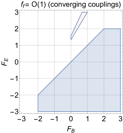
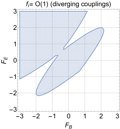
Figure 1: In both plots the shaded area illustrates the allowed region of the parameter space. The left and right plots describe, respectively, the case of converging and diverging gauge couplings.

4.2.3 Bounds exponentially dependent on the number of efolds

The bounds depending exponentially on the number of efolds can be obtained by evaluating the functions ${\mathcal{G}}_{E}(k,a)$, ${\mathcal{G}}_{B}(k,a)$ and ${\mathcal{G}}_{EB}(k,a)$ for $a={\mathcal{O}}(a_{f})$ and by demanding that their relative contribution does not exceed the observational limits, in particular, at the maximal wavenumber of the spectrum. The general expressions of ${\mathcal{G}}_{E}(k,a)$, ${\mathcal{G}}_{B}(k,a)$ and ${\mathcal{G}}_{EB}(k,a)$ can be found, respectively, in Eqs. (4.17), (4.18) and (4.19). Since the same argument can be repeated for these three distinct functions we shall discuss analytically only ${\mathcal{G}}_{E}(k_{max},a_{f})$ and then mention the results for the remaining cases. In the discussion we shall also assume that $\alpha_{E}\neq 0$ and $\alpha_{B}\neq 0$.

From Eq. (4.17) we can easily deduce the following expression:

$${\mathcal{G}}_{E}(k_{max},a_{f})=\frac{1}{\alpha_{E}^{2}}\biggl{(}\frac{k_{max}}{a_{f}H}\biggr{)}^{2\beta_{E}}\biggl{(}\frac{a_{f}}{a_{ex}}\biggr{)}^{2\alpha_{E}-2\mu[|\sigma-1|-1]+2\beta_{E}}.$$ (4.27)

Since, by definition, $k_{max}\eta_{max}={\mathcal{O}}(1)$ we must also have $k_{\max}\tau_{f}={\mathcal{O}}(\sqrt{f_{f}})$. As before the case of converging and diverging gauge couplings can be treated separately. In particular, if $f_{f}={\mathcal{O}}(1)$, Eq. (4.27) implies that the contribution of ${\mathcal{G}}_{E}(k_{max},a_{f})$ will not explode iff:

$$\alpha_{E}-\mu[|\sigma-1|-1]+\beta_{E}<0.$$ (4.28)

But recalling the explicit values of $\alpha_{E}$, $\beta_{E}$, $\mu$ and $\sigma$ the last condition simply means that $F_{E}<2$. The same argument leading to Eqs. (4.27) and (4.28) can be repeated in the case of Eqs. (4.18) and (4.19). The analog of Eq. (4.28) but derived from Eqs. (4.18) and (4.19) will be, respectively,

$$\beta_{B}+\alpha_{B}-\mu[|\sigma|-1]<0,\qquad\beta_{E}+\beta_{B}+\alpha_{E}+\alpha_{B}-\mu[|\sigma|+|\sigma-1|-2]<0.$$ (4.29)

In more explicit term the two conditions of Eq. (4.29) imply respectively $F_{B}+2>0$ and $F_{E}-F_{B}<4$.

In the case of converging couplings the constraints obtained in the present and in the previous subsections are illustrated in Fig. 1. The large shaded area extending through the fourth quadrant of the $(F_{E},\,F_{B})$ plane represents the allowed region of the parameter space where all the constraints are safely satisfied. This region is bounded by the lines $F_{E}=2$, $F_{B}=-2$ and $F_{E}=F_{B}$. The smaller region appearing in the first quadrant illustrates, as an example, a class of magnetogenesis models based on the case of converging gauge couplings [15]: this area corresponds to the region $5F_{B}/3+4/3\leq F_{E}\leq 1.56+2.13F_{B}$ and it is excluded since it does not overlap with the wider region allowed by the constraints on the isotropy of the power spectrum. There are other regions in the first quadrant which are not excluded, including the frontier $F_{E}=F_{B}$. It is however clear that the allowed region extends more towards the fourth quadrant. This means, in practice that the models where $F_{B}>0$ and $F_{E}<0$ are comparatively less constrained.

Let us finally move to the case of diverging gauge couplings and assume for concreteness $f_{i}={\mathcal{O}}(f_{ex})={\mathcal{O}}(1)$. In this case the analog of Eq. (4.27) becomes

$${\mathcal{G}}_{E}(k_{max},a_{f})=\frac{1}{\alpha_{E}^{2}}f_{ex}^{\beta_{E}}\biggl{(}\frac{a_{f}}{a_{ex}}\biggr{)}^{2\mu\beta_{E}+2\alpha_{E}-2\mu[|\sigma-1|-1]+2\beta_{E}},$$ (4.30)

implying that the contribution to the anisotropy is small for $f_{ex}={\mathcal{O}}(1)$ provided

$$\beta_{E}(\mu+1)+\alpha_{E}-\mu[|\sigma-1|-1]<0.$$ (4.31)

The same argument can be applied to ${\mathcal{G}}_{B}(k_{max},af)$ and ${\mathcal{G}}_{EB}(k_{max},a_{f})$. The results are, respectively,

$$(\mu+1)\beta_{B}+\alpha_{B}-\mu[|\sigma|-1]<0,\qquad(\beta_{E}+\beta_{B})(\mu+1)+\alpha_{E}+\alpha_{B}-\mu[|\sigma|+|\sigma-1|-2]<0.$$ (4.32)

In the right plot of Fig. 1 the bounds obtained in the present and in the previous subsections are illustrated in the case of diverging gauge couplings. The various absolute values appearing in Eqs. (4.31) and (4.32) make the frontier of the allowed region less intuitive. It is however clear that the least constrained portion of the parameter space is the second quadrant of the $(F_{E},\,F_{B})$ plane where $F_{B}<0$ but $F_{E}$ is positive. As before there exist limited regions where both rates have the same sign.

5 Concluding remarks

A generalized class of magnetogenesis scenarios based on the relativistic theory of van der Waals interactions implies an asymmetric evolution of the magnetic and electric gauge couplings. As the quantum fluctuations of the gauge fields are amplified, they also gravitate and even if they do not affect the evolution of the background itself, they contribute to the curvature power spectra which have been specifically computed in this paper during a quasi-de Sitter stage of expansion.

Depending on the sensitivity of the derived spectra to the total number of inflationary efolds three different classes of constraints may arise: bounds logarithmically sensitive to the duration of inflation, bounds independent on the duration of inflation and finally bounds which are exponentially sensitive to the number of inflationary efolds. In each of these cases the gauge couplings may either converge towards the end of inflation or diverge from the initial state. If the gauge couplings are converging they are of the same order at the end of inflation and, in this case, the allowed region corresponds, in practice, to the fourth quadrant in the $(F_{B},\,F_{E})$ plane where $F_{B}$ and $F_{E}$ are the rates of the evolution of the gauge couplings in units of the Hubble rate. If the gauge couplings are diverging they are of the same order at the onset of inflation but they can be very different later on. In this case, except for few slices of the parameter space the allowed region falls almost entirely within the second quadrant of the $(F_{B},\,F_{E})$ plane. It is relevant to stress that the scope of the obtained constraints is exactly to pin down the regions of the parameter space where al the potentially large corrections to the curvature power spectra are negligible. In this sense the duration of inflation is immaterial for the allowed regions of the parameter space.

The obtained results clearly show that the constraints point at the case where one of the two gauge couplings contracts and the other expands. On this basis, various classes of magnetogenesis scenarios can be excluded. There remains trajectories in the $(F_{B},\,F_{E})$ plane where the rates can be simultaneously negative or positive (like in the case when $F_{E}\to F_{B}$) but these typically coincide with the boundaries of the allowed region. When the rates have the same sign the gauge couplings may converge at the end of inflation but these models lead to strong anisotropic corrections to the curvature power spectra and seem therefore excluded by the present conclusions. In a complementary perspective the obtained result might also suggest that there exist viable models of magnetogenesis based on the asymmetric evolution of gauge couplings but admitting a strongly anisotropic initial state which becomes isotropic at a later stage. This analysis is beyond the scopes of the present discussion.

References

- [1] D. N. Spergel et al. [WMAP Collaboration] Astrophys. J. Suppl. 148, 175 (2003); D. N. Spergel et al., [WMAP Collaboration] Astrophys. J. Suppl. 170, 377 (2007).
- [2] C. L. Bennett et al. [WMAP Collaboration], Astrophys. J. Suppl. 192, 17 (2011); N. Jarosik et al. [WMAP Collaboration], Astrophys. J. Suppl. 192, 14 (2011); J. L. Weiland et al. [WMAP Collaboration], Astrophys. J. Suppl. 192, 19 (2011).
- [3] D. Larson et al. [WMAP Collaboration], Astrophys. J. Suppl. 192, 16 (2011); B. Gold et al. [WMAP Collaboration], Astrophys. J. Suppl. 192, 15 (2011); E. Komatsu et al. [WMAP Collaboration], Astrophys. J. Suppl. 192, 18 (2011).
- [4] G. Hinshaw et al. [WMAP Collaboration], Astrophys. J. Suppl. 208, 19 (2013); C. L. Bennett et al. [WMAP Collaboration], Astrophys. J. Suppl. 208, 20 (2013).
- [5] P. A. R. Ade et al. [Planck Collaboration], Astron. Astrophys. 571, A23 (2014); P. A. R. Ade et al. [Planck Collaboration], arXiv:1506.07135 [astro-ph.CO].
- [6] L. Ackerman, S. M. Carroll and M. B. Wise, Phys. Rev. D 75, 083502 (2007) [Erratum-ibid. D 80, 069901 (2009)]; A. R. Pullen and M. Kamionkowski, Phys. Rev. D 76 (2007) 103529.
- [7] S. Yokoyama and J. Soda, JCAP 0808, 005 (2008); L. Campanelli, Phys. Rev. D 80, 063006 (2009); N. E. Groeneboom, L. Ackerman, I. K. Wehus and H. K. Eriksen, Astrophys. J. 722, 452 (2010).
- [8] J. Middleton, Class. Quant. Grav. 27, 225013 (2010); J. D. Barrow and S. Hervik, Phys. Rev. D 81, 023513 (2010); S. Kanno, J. Soda and M. -a. Watanabe, JCAP 1012, 024 (2010).
- [9] Y. Z. Ma, G. Efstathiou and A. Challinor, Phys. Rev. D 83, 083005 (2011); T. Q. Do and W. F. Kao, Phys. Rev. D 84, 123009 (2011); T. Q. Do, W. F. Kao and I. -C. Lin, Phys. Rev. D 83, 123002 (2011); S. Hervik, D. F. Mota and M. Thorsrud, JHEP 1111, 146 (2011); S. Bhowmick and S. Mukherji, Mod. Phys. Lett. A 27, 1250009 (2012); N. Bartolo, S. Matarrese, M. Peloso and A. Ricciardone, Phys. Rev. D 87, no. 2, 023504 (2013); D. H. Lyth and M. Karciauskas JCAP 1305, 011 (2013).
- [10] F. Hoyle and J. V. Narlikar, Proc. R. Soc. A, 273, 1 (1963); C. W. Misner, Phys. Rev. Lett. 22, 1071 (1969); Astrophys. J. 151, 431 (1968); M. J. Rees, Phys. Rev. Lett. 28, 1669 (1972).
- [11] A. A. Starobinsky, JETP Lett. 37, 66 (1983);R. M. Wald, Phys. Rev. D 28, 2118 (1983); J. D. Barrow, Phys. Lett. B 187, 12 (1987); J. D. Barrow and O. Gron, Phys. Lett. B 182, 25 (1986). J.D. Barrow, Phys. Rev. D 51, 3113 (1995); Phys. Rev. D 55, 7451 (1997).
- [12] B. Ratra, Astrophys. J. Lett. 391, L1 (1992); M. Gasperini, M. Giovannini, and G. Veneziano, Phys. Rev. Lett. 75, 3796 (1995); M. Giovannini, Phys. Rev. D 56, 3198 (1997); Phys. Rev. D 64, 061301 (2001); Int. J. Mod. Phys. D 13, 391 (2004); K. Bamba and M. Sasaki, JCAP 02, 030 (2007); K. Bamba JCAP 10, 015 (2007); M. Giovannini, Phys. Lett. B 659, 661 (2008).
- [13] K. Bamba, Phys. Rev. D 75 083516 (2007); J. Martin and J. ’i. Yokoyama, JCAP 0801, 025 (2008); M. Giovannini, Lect. Notes Phys. 737, 863 (2008); S. Kanno, J. Soda and M. -a. Watanabe, JCAP 0912, 009 (2009); I. A. Brown, Astrophys. J. 733, 83 (2011); N. Barnaby, R. Namba and M. Peloso, Phys. Rev. D 85, 123523 (2012); T. Fujita and S. Mukohyama, JCAP 1210, 034 (2012); R. Z. Ferreira and J. Ganc, JCAP 1504, no. 04, 029 (2015).
- [14] G. Feinberg and J. Sucher, Phys. Rev. A 2, 2395 (1970); Phys. Rev. D 20, 1717 (1979).
- [15] M. Giovannini, Phys. Rev. D 88, no. 8, 083533 (2013); Phys. Rev. D 92, no. 4, 043521 (2015); Phys. Rev. D 92, no. 12, 121301 (2015).
- [16] S. Deser and C. Teitelboim, Phys. Rev. D 13, 1592 (1976); S. Deser, J. Phys. A 15, 1053 (1982); M. Giovannini, JCAP 1004, 003 (2010).
- [17] M. Giovannini, Phys. Rev. D 85, 101301 (2012); Phys. Rev. D 86, 103009 (2012).
- [18] J. Bardeen, Phys. Rev. D22, 1882 (1980); J. Bardeen, P. Steinhardt, and M. Turner, Phys. Rev. D28, 679 (1983); J. A. Frieman and M. S. Turner, Phys. Rev. D 30, 265 (1984).
- [19] J -c. Hwang, Astrophys. J. 375, 443 (1990); Class. Quant. Grav. 11, 2305 (1994); J. -c. Hwang and H. Noh, Phys. Lett. B 495, 277 (2000).
- [20] J. -c. Hwang and H. Noh, Phys. Rev. D 65, 124010 (2002); Class. Quant. Grav. 19, 527 (2002).
- [21] J. -c. Hwang and H. Noh, Phys. Rev. D 73, 044021 (2006); H. S. Kim, J. -c. Hwang, Phys. Rev. D 74, 043501 (2007).
- [22] V. N. Lukash, Sov. Phys. JETP 52, 807 (1980) [Zh. Eksp. Teor. Fiz. 79, 1601 (1980)]; V. Strokov, Astron. Rep. 51, 431-434 (2007); V. N. Lukash and I. D. Novikov, Lectures on the very early universe in Observational and Physocal Cosmology, II Canary Islands Winter School of Astrophysics, eds. F. Sanchez, M. Collados and R. Rebolo (Cambridge University Press, Cambridge UK, 1992), p. 3.
- [23] M. Giovannini, Phys. Rev. D 76, 103508 (2007); Phys. Rev. D 87, no. 8, 083004 (2013); Phys. Rev. D 90, no. 12, 123513 (2014).
- [24] H. Kodama, M. Sasaki, Prog. Theor. Phys. Suppl. 78, 1-166 (1984); M. Sasaki, Prog. Teor. Phys. 76, 1036 (1986).
- [25] G. V. Chibisov, V. F. Mukhanov, Mon. Not. Roy. Astron. Soc. 200, 535 (1982); V. F. Mukhanov, Sov. Phys. JETP 67, 1297 (1988) [Zh. Eksp. Teor. Fiz. 94, 1 (1988)].
- [26] R. H. Brandenberger, R. Kahn and W. H. Press, Phys. Rev. D 28, 1809 (1983); R. H. Brandenberger and R. Kahn, Phys. Rev. D 29, 2172 (1984).
- [27] J. Valiviita, M. Savelainen, M. Talvitie, H. Kurki-Suonio and S. Rusak, Astrophys. J. 753, 151 (2012); R. Keskitalo, H. Kurki-Suonio, V. Muhonen and J. Valiviita, JCAP 0709, 008 (2007).
- [28] H. Kurki-Suonio, V. Muhonen and J. Valiviita, Phys. Rev. D 71, 063005 (2005); J. Valiviita and V. Muhonen, Phys. Rev. Lett. 91, 131302 (2003).
- [29] S. Weinberg, Phys. Rev. D 72, 043514 (2005); Phys. Rev. D 74, 023508 (2006).
- [30] A. Erdelyi, W. Magnus, F. Obehettinger, and F. Tricomi, Higher Trascendental Functions (Mc Graw-Hill, New York, 1953); M. Abramowitz and I. A. Stegun, Handbook of Mathematical Functions (Dover, New York, 1972).