The Painlevé paradox in contact mechanics

Abstract

The 120-year old so-called Painlevé paradox involves the loss of determinism in models of planar rigid bodies in point contact with a rigid surface, subject to Coulomb-like dry friction. The phenomenon occurs due to coupling between normal and rotational degrees-of-freedom such that the effective normal force becomes attractive rather than repulsive. Despite a rich literature, the forward evolution problem remains unsolved other than in certain restricted cases in 2D with single contact points. Various practical consequences of the theory are revisited, including models for robotic manipulators, and the strange behaviour of chalk when pushed rather than dragged across a blackboard.

Reviewing recent theory, a general formulation is proposed, including a Poisson or energetic impact law. The general problem in 2D with a single point of contact is discussed and cases or inconsistency or indeterminacy enumerated. Strategies to resolve the paradox via contact regularisation are discussed from a dynamical systems point of view. By passing to the infinite stiffness limit and allowing impact without collision, inconsistent and indeterminate cases are shown to be resolvable for all open sets of conditions. However, two unavoidable ambiguities that can be reached in finite time are discussed in detail, so called dynamic jam and reverse chatter. A partial review is given of 2D cases with two points of contact showing how a greater complexity of inconsistency and indeterminacy can arise. Extension to fully three-dimensional analysis is briefly considered and shown to lead to further possible singularities. In conclusion, the ubiquity of the Painlevé paradox is highlighted and open problems are discussed.

KEYWORDS: rigid body; Painlevé paradox; Coulomb friction; impact mechanics; dynamic jam; sprag-slip oscillation; chatter; Zeno phenomenon; reverse chatter; impact without collision; inconsistency; indeterminacy; rational mechanics.

1 Introduction

Paul Painlevé is a truly remarkable figure in the history of science and technology. In mathematics, Painlevé is most closely associated with the family of integrable differential equations and corresponding transcendental functions that bear his name. But there is much more to Painlevé, [8]; he made pivotal contributions to the theory of gravitation, he was possibly the first ever aircraft passenger (taking a seat in the Wright brother’s plane in 1908) and set up the world’s first degree in programme in Aerospace Engineering. His role as Minister of Public Instruction and Inventions, led to him being appointed Prime Minister of France briefly during the First World War, and again in 1924. In the latter stint he was forced to resign after being unable to solve the overriding financial crisis of the time (an uncanny parallel to 21st Century European politics, perhaps).

This paper shall look at the legacy of Painlevé’s work in rigid body mechanics, specifically the rather curious phenomena that are present in models of dry friction. In a series of papers starting in 1895 [61, 62, 63], Painlevé provided simple examples which illustrate a fundamental inconsistency in the laws of Coulomb friction. (Technically, we should refer to Amontons-Coulomb friction, because the laws were first postulated by Amontons at the beginning of the 18th Century, whereas Coulomb’s role was one of experimental verification, see e.g. [33, 19]. As with many unjust attributions in science, Amontons’ name seems to have been dropped from the epithet now used to describe the simplest law of dry friction. In fact, theory that additionally involves solving for the normal force at contact is sometimes called the Signorini-Coulomb model or the Signorini-Amontons-Coulomb $\ldots$, but we shall just refer to Coulomb friction in what follows.) The so-called Painlevé paradox (which, to add more historical accuracy, as Painlevé acknowledges, was first discovered by Jellet [35]) occurs in planar bodies undergoing oblique contact for which there is a sufficiently large coupling between normal and tangential degrees of freedom at the contact point. Such configurations, given sufficiently high coefficient of friction, can reach a point where there is no longer a unique forward simulation — either a multiplicity of possibilities (indeterminacy), or none (inconsistency) — so there is no way to decide what happens next within rigid body mechanics. Further historical remarks on the origins of the Painlevé paradox can be found in the books by Brogliato [10] and and Le Suan Anh [4].

The configuration most closely associated with Painlevé is that of rod falling under gravity whose lowest end is in contact with a horizontal surface and subject to simple Coulomb friction, see Fig. 2. We shall refer to this as the classical Painlevé problem (CPP), although, as pointed out by Leine [43], this was not actually the example that Painlevé considered first (see Sec. 2).

The CPP can be realised using a pencil that is momentarily balanced on its tip on a rough piece of paper attached to a rigid horizontal table. Upon letting go, minor disturbances mean the pencil will have a shallow angle to the vertical and will start to fall. Initially, the tip remains fixed, forming a pivot about which the pencil rotates. Upon reaching some critical angle, the tangential force at the tip will be large enough for the pencil to begin to slip (in the opposite direction to the instantaneous horizontal velocity component of the top). A faint line begins to appear on the paper. As the pencil continues to fall, before it becomes fully horizontal, the angular acceleration will be sufficient to overcome the vertical component of the ground reaction force at the tip. Thus, the tip lifts off and the faint line is terminated. A fraction of a second later, the blunt end of the pencil hits the table, some rattling motion ensues, before the pencil becomes fully horizontal, rolls for a while and comes to rest on the table. No paradox.

What Painlevé realised though is that if the coefficient of friction is large enough (in fact, unrealistically large for an approximately uniform rod like a pencil on anything other than the coarsest sandpaper) then something else can happen. Before the pencil lifts off, it can reach a configuration that is now known as dynamic jam where one cannot decide with certainty what happens next. The pencil tip could lift off in the usual way with an initially infinitesimal normal velocity. Or, the pencil could remain in contact such that the more it tries to lift off, the more it rotates and digs back down into the surface. It is as if there is a negative normal force pulling the tip into the surface. If one adds a rigid impact model, like Newton’s law of restitution, to the mechanical formulation, then such a force causes a so-called impact without collision (IWC) [10, Ch. 5.5], see Sec. 3.2 below. Such an impact involves an impulsive jump to reduce the tip’s slipping velocity to zero and eject it from the surface with a finite normal velocity. We give a more quantitative description of the paradox for the CPP in Sec. 2.2 below.

One of the purposes of this paper is to show that the Painlevé paradox is not just a theoretical curiosity manifest only in “toy” mathematical models of pencils on unrealistically rough surfaces. The consequences of the Painlevé paradox are in fact ubiquitous, even in everyday phenomena. For example, robotic manipulators, pieces of chalk or even your finger are known to judder when they are being pushed across a rough surface [46], see Sec. 2.3 for more details. The phenomenon in question, sometimes referred to sprag-slip oscillation [27], is more complex than mere stick-slip behaviour, as it additionally involves lift-off and impact every cycle. In fact, the somewhat controversial American physicist Walter Lewin is well known for demonstrating how to exploit this effect to draw dotted lines on a blackboard reliably and rapidly by inducing sprag-slip oscillations in the chalk. See Fig. 1

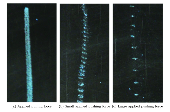
Figure 1: After [25], previously unpublished, reproduced by permission. Three traces left by chalk moved by hand across a rigid blackboard. In all figures the direction of motion is downwards. In (a) there is an acute angle between the chalk’s axis and the velocity vector, whereas in (b) and (c) the angle is obtuse. The difference between (b) and (c) is that an increased normal force is applied in (c).

Nordmark et al [55] demonstrated that such sprag-slip oscillations can arise as a consequence of the Painlevé paradox through an instability that they termed reverse chatter (see Sec. 3 below). This instability involves a sequence of impacts that accumulate backwards in time; rather like watching a video in reverse of a bouncing ball coming to rest. Another everyday phenomenon that can be considered to be a consequence of the Painlevé paradox is how a rigid body can seem to defy gravity by being “wedged” into an overhang (see Fig. 7 below). As we shall show in Sec. 6, there can be subtle effects that involve the interplay between the two contact points, each of which can independently exhibit the Painlevé paradox.

The main aim of this paper is to provide an overview of recent academic work relating to the Painlevé paradox in order to provide some clarity, while keeping in mind the practical implications of the theory. In so doing, we shall also include preliminary new results by the authors and their collaborators, the details of which shall appear elsewhere. Overall, we shall attempt to provide answers to the following two central questions:

Question 1.

For a given rigid body system with contact, in a given state at a given instance of time, is there a uniquely defined forward-time continuation of the dynamics within the formalism of rigid body mechanics? This divides naturally into two subquestions: is any possible forward continuation possible (consistency), and, if so, is it unique (determinacy)?

Question 2.

Given a rigid body system that is not exhibiting the Painlevé paradox at one instance of time, what possible ways can it enter into a Painlevé paradox state at a later in time? Again there are two subquestions: how unlikely is it to enter an inconsistent or indeterminate state; and what happens next?

As we shall show, no complete answer to either question is yet known. Nevertheless, we shall attempt to provide partial answers, restricted to the case of a single point contact in two spatial dimensions. As we shall see though, there are way more possibilities that need consideration in 3D or in the presence of several isolated point contacts, for which we can only provide partial results. For more physically realistic problems with regional (line or patch) contacts, almost nothing is known. Therefore in this paper we shall restrict attention to problems with a finite number of isolated point contacts.

Another aim of this paper is steer a path through the various approaches that have been proposed to resolve the Painlevé paradox from both a practical and a rational, analytic point of view. Our focus is not particularly on numerical methods for simulation in the presence of the paradox, although it is worth pointing out recent results for example in [1, 70, 71]. Nor do we consider control algorithms designed to avoid Painlevé paradoxes in robotic systems, but see e.g. [10, 18] for recent results. Instead, we shall attempt to understand the dynamical consequences of the Painlevé paradox from a mathematical modelling point of view, building on recent understanding of the theory of piecewise-smooth dynamical systems see [20, 42, 16, 15], In fact, it is well known that piecewise-smooth systems of Filippov-type [20] can exhibit nonuniqueness or nonexistence of solutions, see e.g. [20, 5, 34].

Philosophically speaking, the Painlevé paradox is not a puzzle about the real world, but a failure of a theory based on rigid body mechanics and Coulomb friction to provide complete unequivocal descriptions of dynamics. In truth, any physical resolution of the Painlevé paradox tends to involve relaxing some of the assumptions of rigid body mechanics in order to predict what happens next, see Sec. 4. In effect, the Painlevé paradox provides insight into points of extreme sensitivity in rigid body mechanics where additional physics, possibly at the microscale, is required in order to accurately capture the dynamics. Such points of extreme sensitivity are typically going to be observable as points where significant changes can result from minuscule variations of the physical properties or initial states of the bodies involved. A key question to be addressed then is:

Question 3.

Given a rigid body system with contact whose forward evolution is either inconsistent or indeterminate, what is the minimal extra modelling ingredient in order for there to be a unique forward evolution in all inconsistent and indeterminate cases? Which cases can be made uniformly resolvable via this approach; by which we mean, if the additional ingredient to the theory arises through a small parameter $\varepsilon$, does a qualitatively consistent outcome occur uniformly in the limit as $\varepsilon\to 0$?

The rest of this paper is outlined as follows. Section 2 contains a historical introduction to the subject. A mathematical explanation of the paradox is given in terms of the CPP. This is followed by a discussion of the role of different friction laws, a description of other simple configurations that feature the Painlevé paradox and a brief review of the various attempts to resolve the paradox. Section 3 then introduces a general formulation for the simplified case of a planar system with a single contact. An attempt is made to answer Question 1 by enumerating all the different cases that lead to inconsistency or indeterminacy. We also discuss how to augment the formulation by including an impact law, and discuss the possibility of the accumulation of impacts via chatter (also known as the Zeno phenomenon). Section 4 then looks at Question 3 by adding compliance into the model in order to find cases that are uniformly resolvable. Section 5 considers Question 2 for the 2D single contact case; the theory of Génot and Brogliato [22] is reviewed and generalised, to show cases where dynamic jam must occur. We also consider whether the Painlevé paradox can be approached through chatter and consider conditions under which reverse chatter can be triggered. Section 6 considers extensions to the theory for configurations with two or more contact points and starts to enumerate the additional paradoxes that can occur. Section 7 then briefly considers the single-contact problem in 3D, illustrating that a different kind of dynamic jam can occur which does not involve the singularity analysed in [22]. Finally, Section 8 draws conclusions, highlights open problems and and makes philosophical remarks.

2 Historical perspective

Figure 2: The classical Painlevé problem (CPP) for a falling rod.

2.1 The classical Painlevé problem

The CPP, first proposed by Painlevé in 1905 [63], involves a slender rigid rod falling under gravity while in contact with a rigid, stationary, frictional horizontal surface. Suppose the rod has mass $m$ and radius of gyration $r$, that the centre of mass is a distance $\ell$ from the contact point $P$, and that $\lambda_{N}\geq 0$ and $\lambda_{T}$ are the normal and tangential components of contact force. Let $(X,Y)$ be the Cartesian co-ordinates of the rod’s centre of mass within the plane in which it is falling, and $\theta$ be its angle to the horizontal, as depicted in Fig. 2 (note that for convenience we have chosen an angle $\theta$ which is $\pi$ minus the angle of the same name used in [22]). Then, under the usual assumptions of Lagrangian mechanics, the equations of motion can be written as

$$m\ddot{X}=-\mu\lambda_{T},\qquad m\ddot{Y}=-mg+\lambda_{N}\qquad mr^{2}\ddot{\theta}=-\ell(\cos\theta\lambda_{N}+\mu\sin\theta\lambda_{T}).$$ (1)

Let

$$(x,y):=(X+\ell\cos\theta,Y-\ell\sin\theta),\qquad\mbox{and}\quad(u,v):=(\dot{x},\dot{y})$$

represent the generalised tangential and normal co-ordinates and velocities at $P$. Then, $\lambda_{N}$ in (1) can be considered to be a dynamic Lagrange multiplier that is used to maintain the inequality constraint $y\geq 0$. In particular $\lambda_{N}$ and $y$ are said to satisfy a complementarity relation $\lambda_{N}\perp y>0$, which means that at most one of $\lambda_{N}$ and $y$ can be positive (see e.g. [10]). Whenever $y=0$, we assume a simple Coulomb friction law:

$$|\lambda_{T}|\leq\mu|\lambda_{N}|,\qquad\lambda_{T}=-\mu\>\mbox{sign}(u)\lambda_{N}\quad\mbox{for}\>u\neq 0,$$ (2)

where $\mu$ is the coefficient of friction.

Now, suppose there is an initial condition such that the rod is slipping with $u>0$ and $0<\theta<\pi/2$, so that $\lambda_{T}=-\mu\lambda_{N}$. Then, using (1), the normal acceleration can be written as

$$\ddot{y} = \ddot{Y}+\ell(\dot{\theta}^{2}\sin\theta-\ddot{\theta}\cos\theta)\>,$$ (3)

$$= (\ell\dot{\theta}^{2}\sin\theta-g)+\left[1+\frac{\ell^{2}}{r^{2}}\cos^{2}\theta-\mu\cos\theta\sin\theta)\right]\frac{\lambda_{N}}{m}\>,$$

$$:= b(\theta,\dot{\theta})\quad+\quad p^{+}(\theta,\mu)\lambda_{N}\>.$$

Equation (3) describes the dynamics of the CPP in the normal direction at the contact point, in terms of two scalar quantities $b$ which describes the free normal acceleration in the absence of any contact forces and $p^{+}$ which we shall refer to as the “degree of Painlevé -ness” or the Painlevé parameter. In fact, the rest of this paper shall make extensive use of these two dynamic scalar quantities (and a third, $p^{-}$, the equivalent of $p^{+}$ for slipping in the other direction) for quite general classes of contact problems. As we shall see in Sec. 2, $b$ will always be a function of generalised velocities and co-ordinates, whereas for stationary contact surfaces $p^{\pm}$ are functions of position variables and properties of the friction law only.

In the case of the CPP, equation (3) shows that if the rod starts at rest in the near vertical position (with an angle $\theta$ just smaller than $\pi/2$), then clearly $b<0$ and $p^{+}>0$ initially. Moreover $b$ and $p^{+}$ are smooth functions of dynamic variables so, as long as the rod maintains the condition $u>0$ for slip, these quantities will evolve smoothly and preserve their signs for small times. Hence, for sufficiently short times there is a unique normal force

$$\lambda_{N}=-b/p^{+}>0$$ (4)

that makes the normal acceleration in (3) vanish, so that the rod remains in contact while it falls.

Similarly if $\theta$ is initially small and positive so that the rod is close to horizontal then $b<0$ and $p^{+}>0$. However, for intermediate angles, depending on other parameters and velocities, $p^{+}$ and $b$ may in general take either sign. So let us analyse what happens at a time when either $p$ or $b$ smoothly changes sign during motion.

A point where $b$ passes from negative to positive (while $p^{+}$ remains positive) is easy to analyse. This would represent a point at which the rod simply lifts off from the surface. The normal force (4) smoothly tends to zero, the dynamics would lift off into free motion with $y(t)>0$ and $\lambda_{N}=0$.

The case of negative $p^{+}$ is much more unusual. First, consider the possibility of $p^{+}<0$ and $b<0$. Here, the free acceleration $b$ pushes the tip of the rod down towards the surface. However the normal force given by (4) would be negative, which violates our complementarity assumption. A positive reaction force $\lambda_{N}$ would cause acceleration in the same direction as $b$, pushing the rod down further into the surface, precluding any vertical equilibrium. The rod cannot remain in contact with the surface, ergo it must lift off. But it can’t because if we look for free motion with $\lambda_{N}=0$, the free acceleration $b<0$ takes us back into contact. Thus, we have a configuration that is inconsistent, and there is no valid continuation of the motion forwards in time.

Consider instead an initial conditions for which $p^{+}<0$ and $b>0$. Here, in the absence of any contact forces, the rod would simply lift off with $\lambda_{N}=0$. However there is another possibility; there is now a unique non-zero normal force $\lambda_{N}=-b/p>0$ for which the free normal acceleration $b$ is equilibrated. So the rod could remain in contact. Hence, this case is indeterminate, because there is non-uniqueness in possible outcome.

It is useful to consider the conditions under which these paradoxes could occur in the CPP. The condition $p<0$ can be written

$$\mu>\mu_{P}(\theta):=\frac{r^{2}+\ell^{2}\cos^{2}\theta}{\ell^{2}\sin\theta\cos\theta}.$$ (5)

Now, in the case of a uniform rod for which $r^{2}=\frac{1}{3}\ell^{2}$, we see that $\mu_{p}$ is minimised when $\theta=\arctan 2$, in which case we can find the minimum coefficient of friction for which there exists a value for $\theta$ for which $p^{+}<0$, namely $\mu_{P,\rm{min}}=4/3$. Thus, for $\mu>\mu_{P,\rm{min}}$ an interval of angles $\theta$ exists such that $p^{+}$ can be negative.

So what does happen for the falling rod if $\mu>\mu_{P,\rm{min}}$? This question was analysed in detail by Génot and Brogliato [22] (see also [93] for a modern re-interpretation). They show that there is a $\mu_{c}=8/(3\sqrt{3})>4/3=\mu_{P,\rm{min}}$, for the case of the uniform rod, such that for $\mu<\mu_{c}$ there can be no initial condition that approaches $p^{+}=0$ during slipping, the rod must lift off first. But for $\mu>\mu_{c}$ then there is a thin wedge of initial conditions $(\theta,\dot{\theta})$ for which a paradox can be reached. However they show that there can be no entry during forward slipping into regions with $p^{+}<0$, the only way to get there is via reaching a configuration where simultaneously $b=p^{+}=0$, which is precisely what Or & Rimon [60] define as dynamic jam. As we shall see in Sec. 5, the method of Génot and Brogliato, involves rescaling time so that the point $b=p=0$ becomes an equilibrium point in a pseudo phase plain, which can attract an open set of initial conditions. In deference to Génot, we shall call this special point the G-spot. What happens after the G-spot is reached is not clear.

2.2 Is the paradox due to unrealistic friction models?

One simple possible resolution of the Painlevé paradox is that a coefficient of friction $\mu=4/3$ is unrealistically large, with typical values for most materials being significantly less than 1 (although values as large as 2 have been proposed for rubber-on-rubber contacts). This resolution is specious though because it is easy to formulate mechanisms for which $\mu_{P,\rm{min}}$ is significantly smaller. For example, if we allow the rod in the CPP to be non-uniform, then $\mu_{P,\rm{min}}$ is a function of the radius of gyration $r$. Taking the limit that all the mass is concentrated at the centre of mass, then $r\to 0$ and the formula (5) shows that $\mu_{P,\rm{min}}$ becomes vanishingly small in this limit.

Another possible resolution is that the Coulomb friction law is too simplistic and that if a “more realistic” friction model is used, the Painlevé effect will disappear. This may be possible for certain cases and configurations, but seems unlikely in general. For example, Liu et al [46] find the paradox to still be present in a model that has a different dynamic and static coefficient of friction. In addition, there is a trivial indeterminacy if, as is typical for such models, the static coefficient of friction is higher than the dynamic one.

Grigoryan [24] proposes that the CPP can be resolved by replacing the Coulomb friction law with a smoothed version in which $\lambda_{T}$ is a smooth function of $u$ with large finite slope at $u=0$. Philosophically, this is equivalent to replacing dry friction with viscous friction for low velocities. However, he studies only a single rather artificial model, the so-called Painlevé -Klein problem (see Sec. 2.3) and the resolution doesn’t seem to satisfy our definition of uniform resolvability in the limit that the slope tends to infinity. Also, Ivanov [32] claims that such friction laws introduce further non-uniqueness in place of non-existence. If instead we replace Coulomb law with a Stribeck law (see e.g. [41]) in which there is still a jump at $u=0$ but $\mu$ is taken to be a smooth function of $u$, then the above calculations for the CPP can be easily repeated. It is straightforward to show that in principle, there is no impediment to $p^{\pm}$ becoming negative in this case too. The same conclusion holds if $\mu$ is a function of position $x$ or some internal state variable such as in rate-and-state friction models (see [68] and references therein).

There is a rich literature on detailed microscopic friction modelling, indeed tribology is a field in its own right, which we shall not explore further here. Even simple models of tangential friction, ignoring the dynamics in normal directions, can give rise to complex dynamics such as stick-slip vibrations and “squeal”; see for example the reviews [91, 38, 19]. Clearly, when dealing with the Painlevé paradox, the details of what happens in practice are going to depend sensitively on the precise friction characteristics. Nevertheless, it is our contention that the Painlevé paradox is fundamentally due to the nature of the coupling between normal and tangential degrees of freedom, rather than to specific properties of the friction law. Therefore, throughout the rest of this paper, for simplicity, we assume the simple Coulomb law (2), with a single coefficient of friction $\mu$.

Figure 3: The original problem posed by Painlevé of a slipping block

2.3 Other mechanical configurations

In fact, as pointed out by Leine et al [43], the original problem studied by Painlevé in 1895 [61] was not the CPP but that of a planar box slipping down a rough plane that is inclined at a shallow angle to the horizontal; see Fig. 3. The box is assumed to be in point contact at its lowest corner and to be subject to Coulomb friction. As Leine et al show, the simplest model of this problem is actually dynamically equivalent to the CPP (although see [48] for a more general analysis) and the minimum value of friction coefficient required is identical. In particular, just as with the CPP, if we allow the box to have inhomogeneous mass distribution, then $\mu_{P,\rm{min}}$ can in theory be as small as we like.

As mentioned in the introduction, the motion of chalk being pushed across a blackboard is often proposed as a classroom illustration of the Painlevé paradox. In particular, if the chalk is dragged (which would correspond to an angle $\theta$ in the second quadrant if motion is to the right in Fig. 2), then a uniform straight line is generally seen. However, if the angle is in the first quadrant and a large force is applied, then the chalk can undergo a series of hops [25]. Such sprag-slip oscillations were reproduced by Hoffmann and Gaul [27] in various models with compliance at the tip. These oscillations are at least reminiscent of the Painlevé property because lift-off appears to occur despite the chalk being pressed into the board. Such an explanation is not sufficient however because the coefficient of friction for chalk on a blackboard is likely to be significantly less than $\mu_{P,\rm{min}}=4/3$. However, the contact mechanics of chalk, a cylinder that is typically only in contact along part of its end, is likely to be more complex than that of an ideal rod, and we also have to take account of the body forces and controls being applied by the teacher. Moreover, we shall also see in Sec. 5 that another explanation for the onset of the hopping motion, namely reverse chatter, can be triggered upon the transition from stick to slip, even if $p^{\pm}$ remain positive. Indeed Nordmark et al [55] show that an open-loop controller implementing a vander-Pol-like body force to a simple rod model can trigger reverse chatter that saturates into limit-cycle motion.

A laboratory demonstration of sprag-slip oscillations can be made through a pin-on-disk rig, if the the pin is allowed to contact obliquely and to lift off [30]. Such experimental apparatus is often used to categorise friction-induced ‘brake squeal’ vibrations, see for example [12]. Inspired by such systems, Leine et al. [43] studied a so-called frictional impact oscillator, see Fig. 4.

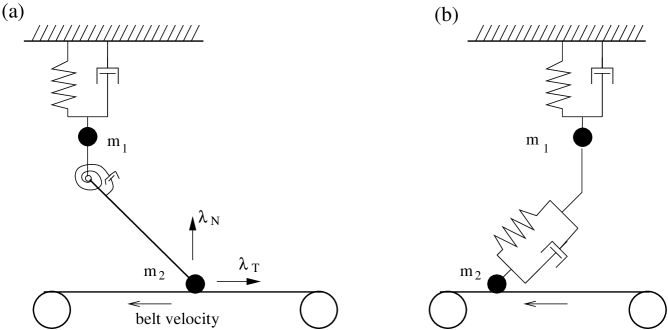
Figure 4: The frictional impact oscillator and its simplification, as studied in [43]

They showed that under suitable choices of parameters the condition for the Painlevé property to hold can be written as $\mu_{P,\rm{min}}=2\sqrt{m_{1}/m_{2}}$, which of course can take arbitrarily small values if the second mass is much heavier than the first. They found that finite-amplitude stable periodic motion can occur in the Painlevé parameter region that comprises phases of free motion, sticking and slipping. The onset of this motion typically occurs via a subcritical Hopf bifurcation from the steady sticking solution.

A related practical manifestation of sprag-slip oscillation is the hopping motion that is sometimes observed in finger-like robotic manipulators [10]. Inspired by this, in a series of papers culminating in [94], Liu, Zhao, Chen and their co-workers have studied theoretically, numerically and experimentally the motion of the two-link robotic manipulator depicted in Fig. 5(a). In particular, in [46] they found precise formula for $\mu_{P,\rm{min}}$, which tends to zero as the height $H\to 0$. They were also able to simulate bouncing motion corresponding to a concatenation of stick, slip, free flight and impact. That such hopping motion is attributable to the Painlevé paradox is now well established in the robotics literature, and work instead has begun to look at how to control such unwanted behaviour (e.g. [18, 45]).

Figure 5: (a) The two-link robotic manipulator [46]. (b) The inverted pendulum on slider [60].

There are also possible applications of these ideas in bio-mimicry of sensing systems. For example, mammals such as rats, have slender tapered rod-like whiskers that repeatedly sweep and tap on a surface at oblique angles, see e.g. [67]. The motion of the tip of a rat’s whisker seems akin to sprag-slip oscillation, but driven by a regular circular motion from the follicle. It would appear that the combined effects of stick-slip and lift-off from the tip, fed back along the whisker enable the rat to sense both texture and compliance of the surface.

Another experimentally amenable Painlevé paradox demonstrator was proposed by Or & Rimon [60], the so-called inverted pendulum on a slider, see Fig. 5(b). They were able to find explicit expressions for initial conditions and parameters that would lead to dynamic jam in such a device. They found the explicit expression $\mu_{P,\rm{min}}=\sqrt{(2(1+m_{1}/m_{2})(1+\rho_{2}/r_{2})-1)^{2}-1}$, which can be chosen to be experimentally accessible by choosing appropriate values for the configuration constants $m_{1}$, $m_{2}$ $r_{2}$ and $\rho_{2}$.

A less explored, but potentially industrially important area in which the Painlevé paradox can apply is in rotating machinery. Here there may be large coupling between normal and tangential degrees of freedom due to gyroscopic forces. For example Wilms & Cohen [90] report that the Painlevé effect can be seen the motion of rotating shaft whose bearing is subject to coulomb friction. Kozlov [39] studies a brake shoe problem that exhibits the Painlevé paradox, which he claims was resolved by Neimark and co-workers [52] by introducing longitudinal and transverse elasticity, see Sec. 2.4.

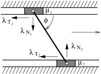
Figure 6: The Painlevé-Klein problem

All of the above examples correspond to cases with a single point contact. There is less in the literature on the Painlevé paradox occurring in problems with multiple contacts. The Russian literature tends to use as the canonical model, not the CPP but the so-called Painlevé-Klein problem, see [32, 52, 88, 24, 3]. A good summary discussion of work on this problem is given in the book by Anh [4]. The problem involves a rod that is wedged between two rigid constraints with Coulomb friction applying at each, see Fig. 6. In fact, like the slipping block in Fig. 3, this problem predates the CPP, going back to Painlevé’s original work [61]. Here it can be shown that there are multiple cases to analyse depending on whether lift-off is allowed to occur at either of the contacts. The simplest case is where both ends are assumed to always remain in contact, so that the normal forces $\Lambda_{N_{1,2}}$ can take either sign. Such frictional contacts are termed bilateral. Then, using the notation in Fig. 6, paradoxes can be shown to occur whenever

$$|\mu_{2}-\mu_{1}|\leq\cot\phi.$$

In particular if the rod is pulled such that a stick-slip transition is reached, then if $\mu_{1}=\mu_{2}$ one can’t decide which end will slip first. Ivanov [32] analyses cases where either or both of the constraints are unilateral, showing that there is a much richer complexity of possibilities, depending on the relative sizes of the two coefficients of friction. In general, we shall consider only unilateral constraints in what follows and, for the most part, mechanisms with just a single contact point. Extension to multiple contact points is the subject of Sec. 6, where we will specifically point out several different cases of nonuniqueness, as illustrated in Fig. 7.

Figure 7: (Adapted from [85]). Two examples of ambiguous equilibria involving planar rigid bodies with two contact points. (Left) a rigid two-dimensional heavy block between two skew walls where both contacts in stick are consistent provided the coefficient of friction is high enough. (Right) a body resting on two points in which the left-hand contact is slippery, while there is sufficiently high friction at right-hand contact. Here there is indeterminacy between static equilibrium and an accelerating motion in which the left-hand contact point slips and the right-hand contact point lifts off. The mode names refer to the notation introduced in Sec. 6 below.

Or [57] studied practical configurations with multiple points that can exhibit the Painlevé paradox, simple passive walking mechanisms such as the rimless wheel and the compass biped, see Fig. 8. He argues that many walking models assume frictional sticking contact of the leg with the ground. Allowing perturbations that involve foot slippage, he shows that regular gait periodic solutions can be subject to an instability that is closely related to dynamic jam. Dynamical consequences of this instability and the ensuing stable dynamical behaviours are considered in detail in [21].

Figure 8: (a) The rimless wheel and (b) the compass biped configurations studied in [57, 21].

2.4 Resolutions of the paradox; regularisation and impact mechanics

Various attempts to resolve the Painlevé paradox have taken place in the intervening 120 years since Painlevé first published his work. These attempts took on new vigour in the 1990s due to the development of rigorous methods using the complementarity framework for rigid body mechanics and the theory of differential inclusions; see for example [76] for a review. One idea, due to the influential French mathematician Moreau [51], is to solve the problem via simulation, using specific time-stepping numerical discretisation schemes designed for linear complementarity problems. Using this idea Stewart [74, 75] provided a resolution in the form of a rigorous proof that a time-stepping schemes exist that are well posed and, by taking the zero-stepsize limit, one has a proof that mechanics in the Painlevé regime is consistent. That is, there is always a well defined forward-time evolution of the dynamics from any reachable configuration. However, this approach does not deal with the problem of indeterminacy that is, one can have non-uniqueness in the forward time dynamics. Stewart’s result also does not resolve the paradox in the sense of the three Questions posed in the introduction as it does not consider the nature of the solution in the limit as the stepsize tends to zero.

Another way to resolve the Painlevé paradox is to break the formalism of rigid body mechanics and to introduce some new physics, for example by including dynamics in the normal direction, thus smoothing the problem. This approach seems to be prominent in the Soviet literature, following the publication of the Russian translation of Painlevé’s work in 1954 (see e.g. [3, 32, 52, 4] and references therein). For example, Neimark and Smirnova [52] propose that the normal force should be considered as a dynamical variable that evolves on a fast timescale. They argue that the dynamics of the Painlevé-Klein problem would then feature “contrast structures” by which they mean two-timescale dynamics that can converge to periodic solutions with well-defined rapid jumps in tangential velocity. Without this regularisation they claim that only constant acceleration solutions can be found in the Painlevé-Klein problem. This general approach can be referred to as contact regularisation, which treats the rigid body limit of a compliant formulation as a singular perturbation problem. A good general discussion of contact regularisation and its application to the Painlevé-Klein problem in particular can be found in [4]. In Sec. 4 below we show how such contact regularisation in the normal direction can lead to answers to Questions 2 and 3 by taking the limit that the stiffness, following arguments in [55].

Most authors agree that a complete understanding of the Painlevé paradox requires consideration of impact. That is, what would happen in the CPP if the rod is first dropped onto the surface so that it first makes contact with $v<0$ and $b>0$. In general, contact will not be maintained, but the body will bounce. Even before the advent of classical mechanics, a great deal of effort was made to understand collisional impact, see [79, Appendix A] for an historical account. Within a rigid-body framework, the loss of energy in the impact event is usually modelled as a zero-time process involving impulsive forces. Impacts for which there is no coupling between tangential and normal degrees of freedom during contact are most simply captured by a Newtonian restitution law

$$v^{+}=-rv^{-},\qquad r\in[0,1].$$ (6)

A completely elastic (conservative) collision corresponds to a coefficient of restitution $r=1$, and a completely inelastic case to $r=0$. Of course, even this classical law is an approximation, as Newtonian coefficients of restitution are approximations that depend not only on the properties of the contacting materials but on how the geometry of the impacting bodies allow wave energy to be dissipated, see e.g. [50, 81].

The Painlevé paradox involves oblique impacts, which involve instantaneous changes in the tangential as well as normal velocity. Unlike purely normal impacts, it appears from the literature that different modelling choices can be made in order to resolve oblique impacts. within a rigid-body framework. First, it is tempting to simply ignore the tangential dynamics during impact and apply (6) in the normal direction. However, this can lead to an increase in energy during impact [36, 13]. Another obvious idea is to introduce a second model parameter, — a “transverse coefficient of restitution” [65] or a fixed “impulse ratio” between the tangential and normal velocity jumps [9] but this can similarly be shown to lead to energy gain in Painlevé paradox situations [11]. Chatterjee and Ruina [13] discuss which closed form expressions for impact lead to oblique impacts that are energetically consistent.

As pointed out in [13], the problem of many simplistic approaches to modelling oblique impact is that they ignore the fact that during the impact process a transition from slip to stick can occur. In fact, as argued by Stronge [79], see also Sec. 3.2 below, consistent impact laws can only be reached in all circumstances by solving the dynamic problem of compression followed by restitution, in a rapid timescale in which the impulsive forces become of $O(1)$, fully resolving any transitions between slip. This is a form of contact regularisation that makes impact resolvable by passing to the limit that its duration is infinitesimal. The question then arises as to what is the analogue of the coefficient of restitution for such a process. Or, more precisely, when do we decide that the restitution phase has terminated? Various alternatives are possible, with the simplest one, based on a condition on normal velocities akin to (6) being easily shown to be inconsistent, see [69] for a comparison. One possible resolution is to use Poisson’s kinetic restitution law [66], see also [37, 6] that supposes there is a ratio between the normal impulse in compression to that in restitution. Alternatively, Stronge [78] proposed an energetic restitution law that considers the ratio of normal work done in compression to that in restitution. Stronge’s law has the benefit that by construction, it is energetically consistent that is, the impact must be dissipative if the energetic coefficient of restitution is strictly less than unity, and is necessarily conservative if it equals unity. Nevertheless, energetic consistency can also be proved to hold for the Poisson law [31, 13]. When the Painlevé property holds, both laws give the possibility of impact without collision (IWC) [22, 76]. That is, where a finite outgoing normal velocity ensues from a zero incoming velocity. As we shall see in Sec. 3.2, such events can provide a resolution to the inconsistent case of the Painlevé paradox.

There are relatively few studies that analyse or simulate configurations exhibiting the Painlevé property with models that incorporate both continuous contact and impact. For example, in one of the first papers to analyse the Painlevé phenomenon from the perspective of non-smooth bifurcations, Leine et al. [43] assumed a coefficient of restitution equal to zero. This was improved upon by Liu et al. [46] who simulated similar hopping motion using a non-zero Poisson coefficient of restitution $r_{p}$, but their analysis of periodic motion is restricted to the case case $r_{p}=0$.

In contrast, Stronge and co-workers [73, 77, 80] consider in detail the transitions that occur during impact, but ignoring the case of IWC. They find that there are no paradoxes. Indeed, this should not be surprising, because, as shown in [53, 78, 17] explicit expressions for the outgoing velocity in terms of the incoming velocity can be obtained for each of the Newtonian, Poisson and Stronge restitution laws, for all possible itineraries of slip and stick during compression and restitution.

3 General formulation for planar single contact case

This section is devoted to the answering Question 1 in the restricted case of planar systems with a single point of contact, without introducing any additional ingredients to the rigid-body formulation. We shall deal with typical cases, given by open (generic) conditions on parameters. Cases that are on the boundary of these open regions are dealt with in Sec. 4.

Consider a planar mechanical system with a single point whose dynamics is governed by the Lagrangian system

$$M\left(q,t\right)\ddot{q}=f(q,\dot{q},t)+\lambda_{T}c(q,t)+\lambda_{N}d(q,t).$$ (7)

Here $q\in{\mathbb{R}}^{n}$ is a vector of generalised co-ordinates, with $\dot{q}$ the vector of corresponding generalised velocities, $f$ contains all body forces, including potentially both conservative and dissipative forces, and $\lambda_{T}$ and $\lambda_{N}\geq 0$ represent the magnitudes of tangential and normal forces respectively that act in the directions corresponding to the generalised co-ordinate vectors $c(q)$ and $d(q)$. $M(q)$ is a mass matrix which we assume to be positive definite for all admissible configurations $q$. Each of $M$, $f$, $c$ and $d$ is assumed to be a sufficiently smooth function of its arguments.

Let $(x(q),y(q))$ be the co-ordinates associated with the $c$ and $d$ directions so that the constraint is given by $y\geq 0$, and let $\dot{x}=u$ and $\dot{y}=v$ be the tangential and normal velocities respectively. Then, we can project (7) onto tangential and normal directions to obtain the scalar equations

$$\dot{u} =a\left(q,\dot{q},t\right)+\lambda_{T}A\left(q,t\right)+\lambda_{N}B\left(q,t\right),$$ (8)

$$\dot{v} =b\left(q,\dot{q},t\right)+\lambda_{T}B\left(q,t\right)+\lambda_{N}C\left(q,t\right),$$ (9)

where the scalars $a$, $b$, $A$, $B$, $C$, $D$ are given by

$$a=c^{T}f,\quad b=d^{T}f,\quad A=c^{T}M^{-1}c,$$

$$B=c^{T}M^{-1}d\quad\mbox{and}\quad C=d^{T}M^{-1}d.$$

The scalars $\lambda_{N}$ and $\lambda_{T}$ are Lagrange multipliers that must be solved for under different assumptions on the mode of motion. Whenever $y>0$ or $v>y=0$, we have free motion for which necessarily $\lambda_{N}=\lambda_{T}=0$. During contact $y=v=0$, we suppose that Coulomb friction (2) applies.

Note that because $AC-B^{2}$ is the determinant of a $2\times 2$ submatrix of $M^{-1}$ and $A$ and $C$ are diagonal elements in an appropriate basis, then the positive definiteness of $M$ implies that

$$A>0,\quad C>0,\quad AC-B^{2}>0,$$ (10)

whereas $a$, $b$ and $B$ are in general not sign constrained. Moreover from (10), simple algebraic manipulation shows that at most one of

$$\mu A-B,\quad\mu A+B,\quad C-\mu B,\quad C+\mu B$$ (11)

can be non-positive, which will be important in what follows. The case $B=0$ corresponds to there being no coupling between the normal and tangential forces during contact. The Painlevé paradox can occur whenever $|B|$ is sufficiently large. Note, from the CPP example (1), in the case of a uniform rod, nondimensionalisation using length scale $\ell$, time scale $\sqrt{\ell/g}$ and mass scale $m$, gives $a=-\dot{\theta^{2}}\cos\theta$, $b=\dot{\theta^{2}}\sin\theta-1$, $A=1+3\sin^{2}\theta$, $B=3\sin\theta\cos\theta$, $C=1+3\cos^{2}\theta$.

3.1 Consistency of contact motion

Sustained contact occurs when $y=v=0$, from which we can distinguish four generic possible modes of motion; lift-off into free motion ($F$), stick ($T$) and slip either in the positive $u$ ($S_{+}$), or negative $u$ ($S_{-}$) direction. To determine which mode is consistent for any configuration, we can apply a three step algorithm, see Table 1:

1. check kinematic admissibility;

2. find contact forces and accelerations using equations of motion and equality constraints;

3. check consistency conditions.

Let us now consider the details of the consistency analysis for the four contact modes:

Free motion

occurs when $\lambda_{N}=\lambda_{T}=0$, which implies $\dot{v}=b$. The consistency condition $\dot{v}=0$ is satisfied if $b>0$.

Positive slip

occurs when $y=0$, $v=0$, $\lambda_{N}>0$ and $u\geq 0$. We now have the full friction force so that $\lambda_{T}=-\mu\lambda_{N}$ and hence to sustain contact we must have

$$\dot{v}=b+(C-\mu B)\lambda_{N}=0.$$ (12)

We can define the positive Painlevé parameter

$$p^{+}:=C-\mu B,$$ (13)

and rewrite (12) as

$$\dot{v}=b+p^{+}\lambda_{N}=0,,$$ (14)

which implies

$$\lambda_{N}=-\frac{b}{p^{+}},\qquad\dot{u}=a-b\frac{(B-\mu A)}{p^{+}}.$$ (15)

Thus, the consistency condition $\lambda_{N}\geq 0$ becomes that $b$ and $p^{+}$ should have opposite sign (with $p^{+}=0$ leading to $\lambda_{N}$ being undefined). We say that the Painlevé paradox for positive slip occurs when $p^{+}<0$. Note that the additional consistency condition for the case $u=0$ is that $\dot{u}$ given by the second equation in (15) should be positive, that is

$$a-b\frac{(B-\mu A)}{p^{+}}>0.$$ (16)

Negative slip

similarly occurs when $y=0$, $v=0$, $\lambda_{N}>0$ and $u\leq 0$, $\lambda_{T}=\mu\lambda_{N}$ and

$$\dot{v}=b+p^{-}\lambda_{N}=0.$$ (17)

where the Painlevé parameter for negative slip is

$$p^{-}:=C+\mu B.$$ (18)

So, we have

$$\lambda_{N}=-\frac{b}{p^{-}},\qquad\dot{u}=a-b\frac{(B+\mu A)}{p^{-}},$$ (19)

and hence the consistency condition for negative slip is that $b$ and $p^{-}$ should have opposite sign, and we identify the case $p^{-}<0$ as representing the Painlevé paradox for negative slip. Again there is an extra consistency condition on $\dot{u}$ in the case $u=0$, that is,

$$a-b\frac{(B+\mu A)}{p^{-}}<0.$$ (20)

Stick

represents a mode for which $y=0$, $v=0$, $\lambda_{N}>0$, $u=0$, and $|\lambda_{T}|<\mu\lambda_{N}$. In order to sustain stick we must have $\dot{u}=\dot{v}=0$ from which we can explicitly obtain

$$\left(\lambda_{T},\lambda_{N}\right)=\left(\frac{bB-aC}{AC-B^{2}},\frac{aB-Ab}{AC-B^{2}}\right).$$ (21)

The consistency condition $|\lambda_{T}|<\mu\lambda_{N}$ to remain in stick, can thus be written as

$$a(C-\mu B)+b(\mu A-B)<0,\quad-a(C+\mu B)+b(\mu A+B)<0.$$ (22)

By analogy with the 3D case, the conditions are sometimes said to define the interior of the friction cone in the $(a,b)$-plane. This region is represented by the vertically hashed area in Fig. 9. Note the shape of the cone depends on the signs of $p^{\pm}$ and the additional parameters

$$k^{+}:=\mu A-B,\qquad k^{-}:=\mu A+B.$$ (23)

(Note a change in sign convention for the definition of $k^{+}$ from [53] where it was called $-k_{T}^{+}$.)

Mode	pos. Slip ($S_{+}$)	neg. Slip ($S_{-}$)	sTick ($T$)	lift ofF ($F$)
kinematic admissibility	$y=v=0$ and $u\geq 0$	$y=v=0$ and $u\leq 0$	$y=v=0$ and $u=0$	$y>0$; or $y=0$ and $v\geq 0$
equality constraints	$\lambda_{T}=-\mu\lambda_{N}$ and $\dot{v}=0$	$\lambda_{T}=\mu\lambda_{N}$ and $\dot{v}=0$	$\dot{u}=\dot{v}=0$	$\lambda_{N}=\lambda_{T}=0$
consistency	$\lambda_{N}\geq 0$; and if $u=0$: $\dot{u}>0$	$\lambda_{N}\geq 0$; and if $u=0$: $\dot{u}<0$	$\lambda_{N}\geq 0$; and $|\lambda_{T}|\leq\mu\lambda_{N}$	if $y=v=0$: $\dot{v}>0$

Table 1: Constraints of the four contact modes.

All four parameters $p^{\pm}$, $k^{\pm}$ are positive in the case $B=0$ and, owing to (11), at most one of them can be negative in generally. If one the $k$ parameters is negative then we have the case illustrated in the bottom left panel of Fig. 9 in which the conditions for stick are completely contained within one quadrant. If instead one of the $p$ parameters is negative then we have the case in the bottom right panel in which the stick region extends into the lift-off zone $b>0$. In this latter case there is a range of $a$-values for which stick and slip are consistent even if $b>0$.

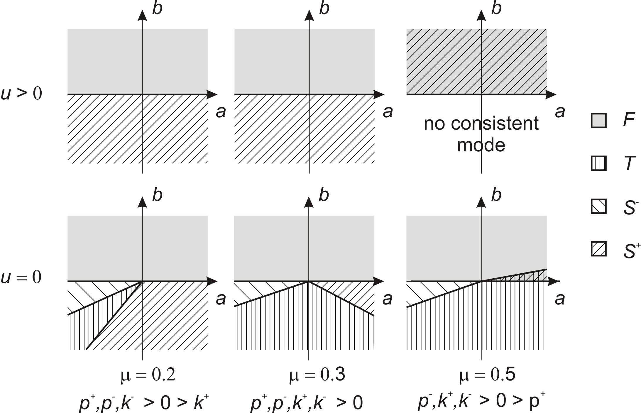
Figure 9: Consistency regions of the four contact modes in the plane of parameters $a$ and $b$ at three values of the coefficient of friction $\mu$, for sustained contact $y=v=0$ with positive tangential velocity ($u>0$, top) and with stationary contact ($u=0$, bottom). The case illustrated is for $A=1.1$; $B=0.3$; $C=0.1$. The largest value of $\mu$ induces $p^{+}<0$ for which there are regions of indeterminacy and inconsistency in the parameter plane.

	I:   $u>0$	II:   $u=0$	III:   $u<0$
(i): $b>0$, $p^{+}>0$, $p^{-}>0$	$F$	$F$	$F$
(ii): $b>0$, $p^{+}>0$, $p^{-}<0$	$F$	$F$ or ($F$ and $T$ and $S_{-}$)	$F$ and $S_{-}$
(iii): $b>0$, $p^{+}<0$, $p^{-}>0$	$F$ and $S_{+}$	$F$ or ($F$ and $T$ and $S_{+}$)	$F$
(iv): $b<0$, $p^{+}>0$, $p^{-}>0$	$S_{+}$	$T$ or $S_{+}$ or $S_{-}$	$S_{-}$
(v): $b<0$, $p^{+}>0$, $p^{-}<0$	$S_{+}$	$S_{+}$ or $T$	—
(vi): $b<0$, $p^{+}<0$, $p^{-}>0$	—	$S_{-}$ or $T$	$S_{-}$

Table 2: Consistency of the contact modes depending on the signs of $b$, $u$, $p^{+}$, $p^{-}$. Here ‘or’ is exclusive and which mode occurs depends on other inequality conditions between $a$, $b$, $A$, $B$ and $C$; specifically, stick occurs if and only $a$ and $b$ lie in the interior of the friction cone given by (22). However ‘and’ is inclusive and represents indeterminacy. A ‘—’ symbol is used to denote cases where there is no consistent mode.

The results of this consistency analysis are summarised in Table 2 and illustrated in Fig. 9. Note the inconsistency in cells I(vi) and III(v) of the table. These cases are symmetric with respect to each other under the transformation $x\to-x$, $B\to-B$, which maps forward to backward slip, so without loss of generality we consider the case for positive slip; $y=v=0$, $b<0$ $p^{+}>0$, $u>0$. Here, stick is not possible since $u>0$, nor is lift-off into free motion, because the free acceleration $b$ is in the direction towards the constraint surface $y=0$. Negative slip is not possible because $u>0$, and finally positive slip is not possible because $\lambda_{N}$ given by (4) would be negative. To resolve what must happen in such cases, in practice we need to consider the possibility of an IWC, which will do in the next subsection.

There are also two different types of indeterminacy, comprising four cases in all. The first type is indeterminacy between slip and lift-off in cells I(iii) and III(ii), with these two cases being symmetric with respect to each other under the transformation that maps positive slip to negative slip. So, without loss of generality, consider positive slip; that is $y=v=0$, $b>0$, $p^{+}>0$, $u>0$. Here, stick is not possible because $u>0$ but lift off is possible, as is positive slip, with $\lambda_{N}$ given by (4) being positive because it is the ratio of two negative quantities. The other type of indeterminacy is between liftoff, stick and slip, in cells II(ii) and II(iii) where $b>0$ and $a$ is such that we lie inside the friction cone (that is, inside the multi-shaded region of the bottom-right panel of Fig. 9). Here lift-off is possible because $b>0$. Additionally though, a positive normal force $\lambda_{N}$ can be found such that the conditions for stick are satisfied. In addition, a larger normal force $\lambda_{N}$ exists such that slip is possible for the direction corresponding to the parameter $p^{\pm}$ that is negative. These cases of indeterminacy cannot be resolved in general (in the sense of Question 1 in the introduction), but can be resolved in terms of their stability (in the sense of Question 2) see Sec. 4 below.

3.2 Impact

As discussed in Sec. 2.4, the discussion of the Painlevé paradox in a rigid body framework requires the inclusion of an impact law. Indeed, if contact regularisation is included in the normal direction, the necessity of IWC is easily concluded (see e.g. [52]). Following [79, 53] we shall introduce a formalism for the impact phase as something occurring on an asymptotically faster timescale $\tau=t/\varepsilon$ in which contact forces become asymptotically large $(|\lambda_{T}|,\lambda_{N}=\mathcal{O}(\epsilon^{-1}))$ such that velocities $(u,v)$ (and more generally $\dot{q}$) can vary by an $O(1)$ amount, but the generalised coordinates $q$ remain constant. We shall introduce a notation that the pre- and post-impact velocities are represented using superscripts ^- and ⁺ respectively.

Then, if we define the rescaled contact forces $\Lambda_{T,N}=\varepsilon\lambda_{T,N}$ then from (8), (9) we get in

$$\frac{du}{d\tau} =\Lambda_{T}A+\Lambda_{N}B+O(\varepsilon),$$ (24)

$$\frac{du}{d\tau} =\Lambda_{T}B+\Lambda_{N}C+O(\varepsilon),$$ (25)

where $A$, $B$ and $C$ are now constant during the impact process. Moreover, we can replace time $\tau$ with units of the normal impulse [79]

$$I_{N}=\int\Lambda_{N}d\tau$$

which is a monotonically increasing function of $\tau$. Then we get

$$u^{\prime} =(\Lambda_{T}/\Lambda_{N})A+B+O(\varepsilon),$$

$$v^{\prime} =(\Lambda_{T}/\Lambda_{N})B+C+O(\varepsilon),$$

where a prime represents $\frac{d}{dI_{N}}$. These equations, after substitution from the Coulomb friction law (2) with $\lambda_{T,N}$ replaced by $\Lambda_{T,N}$, lead to leading order to explicit affine equations for $u(I_{N})$ and $v(I_{N})$. In fact, as shown in [53], the motion is always along straight lines in the $(u,v)$-plane, with corners occurring at transitions between slip and stick during the impact process; see Fig. 10 for examples.

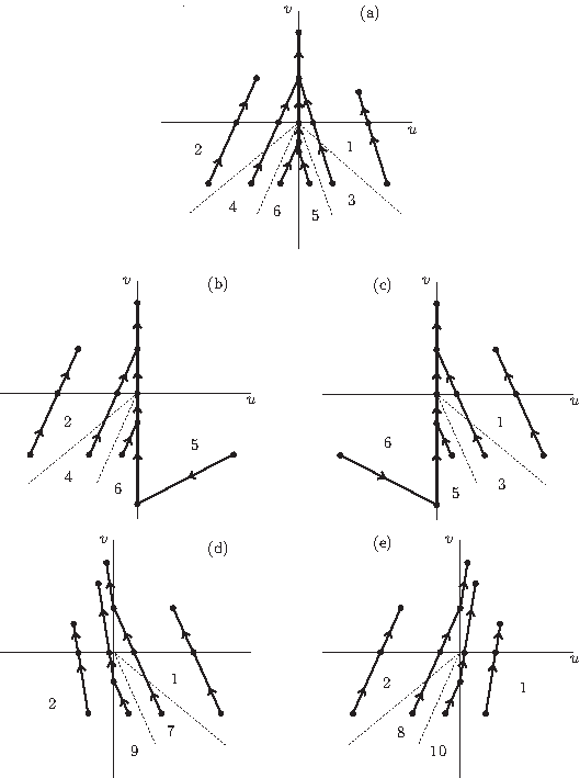
Figure 10: After [53], reproduced with permission. Graphical description of the impact process, in: the typical case (a) $p^{+},p^{-},k^{+},k^{-}>0$; the Painlevé cases (b) $p^{+}<0$, (b) $p^{-}<0$; or the slip reversal cases (c) $k^{-}<0$, (d) $k^{+}<0$. In each case the mapping is depicted from an incoming velocity pair $(u^{-},v^{-})$ with $v^{-}\leq 0$ to an outgoing pair $(u^{+},v^{+})$ with $v^{+}>0$. The dashed lines represent boundaries between regions in $(u^{-},v^{-})$-space, represented by a different numerical symbols, in which the map takes a different functional form.

The impact process can then be defined as a composite mapping

$$(u^{-},v^{-})\mapsto_{\mbox{compression phase}}(u^{*},0)\mapsto_{\mbox{restitution phase}}(u^{+},v^{+}),$$ (26)

where in each of the compression and restitution phases one needs to account for possible transitions from slip to stick. It is possible to then define a composite closed from expression for the impact map under different combinations of the signs of $p^{+}$, $p^{-}$, $k^{+}$ and $k^{-}$ defined in (13), (18) and (23), and different conditions on the ratio $u^{-}/v^{-}$ between initial velocities. The results are summarised in Fig. 10; detailed calculations under the assumption of an energetic impact law in [53]. In that case we deem an impact to be over when the normal kinetic energy gained during restitution is $-r^{2}$ times the normal kinetic energy lost during compression. This defines an energetic coefficient of restitution $r=r_{e}$. Similar calculations can be carried out explicitly for the Poisson impact law (see e.g. [13]), the only difference being the point at which the restitution phase is deemed to be over. In that case, restitution is deemed to end when the normal impulse in $I_{N}=\int\Lambda_{N}$ gained during restitution is $r$ times the normal impulse gained during compression, which defines a Poisson coefficient of restitution $r=r_{p}$

Note that the assumption that the same Coulomb friction law should apply during the impact phase as in the $O(1)$-timescale motion is a modelling assumption that doesn’t necessarily follow. For example, when modelling impact in a so-called superball, it has been suggested that a friction law is used where the transition between stick and slip occurs not at $u=0$ but for some non-zero $u>0$ [14]. In truth, frictional forces are temperature, timescale and spacescale dependent, see e.g. [91]. The impact process (26) can in principle be defined under different friction laws, or indeed for a different value of the coefficient of friction $\mu_{I}$ than for the $O(1)$-timescale motion.

Note that in general $v^{-}<0$, but that in parameter regions 5(b) or 6(c) in the figure, the impact equations also have a solution if $v^{-}=0$. These regions correspond precisely to when either of the Painlevé parameters $p^{+}$ or $p^{-}$ is negative and the pre-impacting motion is in slip of the correct sign ($u>0$ or $u<0$ respectively). In particular these two parameter regions are precisely where an impact can occur with $v^{-}=0$, that is an impact without collision. Note these cases map to the inconsistent and the indeterminate cases of Table 2 with $u\neq 0$. Thus, we have at least one forward solution in all cases.

Also note from the Fig. 10 that impact can result in the phenomenon of slip reversal, that is where $u^{+}u^{-}<0$ so that the body will enter impact with slipping in one direction and exit slipping in the other. This phenomenon occurs in parameter regions 7-10 of the figure which occurs when one of the parameters $k^{+}$ or $k^{-}$ is negative.

3.3 Chattering and inverse chattering

Chattering, also known as the Zeno phenomenon, is the process by which an infinite sequence of impacts occurs in a finite period of time. In single degree-of-freedom mechanical systems, such a sequence can easily occur whenever there is a coefficient of restitution less than unity and acceleration that is towards the contact for a sufficiently long period of time. The canonical example of such an impact sequence occurs when dropping an elastic ball on a rigid floor, and can also occur in general impact oscillators, see [15, 56] and references therein. For systems with oblique impacts, chattering sequences can also converge in reverse time.

To understand this phenomenon, following [55] we define a chattering sequence as a rapid sequence of impacts interspersed with brief intervals of free flight. To analyse such a sequence, we consider a single iterate that starts immediately prior to the $n$th impact, as defined in the previous section, and ends immediately prior to the $(n+1)$st impact. This defines a bounce mapping

$$g:\>\begin{pmatrix}u_{n}^{-}\\ v_{n}^{-}\end{pmatrix}\mapsto_{\mbox{impact map $i$}}\begin{pmatrix}u_{n}^{+}\\ v_{n}^{+}\end{pmatrix}\mapsto_{\mbox{free flight map $f$}}\begin{pmatrix}u_{n+1}^{-}\\ v_{n+1}^{-}\end{pmatrix}.$$ (27)

Now, it is easy to see that for chatter to occur at all we need the free normal acceleration to be towards the contact, that is $b<0$. Moreover, we assume that the impact we are analysing is sufficiently far into the sequence that the normal velocities are small. Then the time spent in free flight is

$$t_{n}=-2(v_{n}^{+}/b)+O[(v_{n}^{+})^{2}].$$ (28)

Therefore we can write the free flight map, up to order $(v_{n}^{+})^{2}$ as

$$f:\begin{pmatrix}u_{n}^{+}\\ v_{n}^{-}\end{pmatrix}\mapsto\begin{pmatrix}u_{n}^{+}-(2a/b)v_{n}^{+}\\ -v_{n}^{+}\end{pmatrix},$$

and define an effective normal coefficient of restitution via the ratio

$$e:=\frac{v_{n+1}^{-}}{v_{n}^{-}}.$$ (29)

Note that because $v_{n+1}^{-}=-v_{n}^{+}$ this ratio $e$ is precisely the Newtonian coefficient of restitution, which ignores the motion in the tangential direction.

If $e<1$ then we have a chattering sequence that accumulates as $n\to\infty$, and the times of flight $t_{n}$ represent a geometric sequence, whose sum converges to a finite limit which is proportional to $(1-e)^{-1}$. In the context of impact oscillators this process is sometimes called a complete chattering sequence (see [15, Ch.6] and references therein); in the context of hybrid systems, the limit point of this process is sometimes called a Zeno point (see e.g. [40]). The process is like that of a bouncing ball coming to rest in finite time. For non-oblique impacts (i.e. when $B=0$) it is possible to show that $e=r$, a property that still holds true whenever there are no transitions from slip to stick during the impact process (in regions 1,2 of Fig. 10).

However, Nordmark et al [55] show that under situations where there is a transition from slip to stick during impact, then it is possible to find configurations such that $e>1$, even if the energetic coefficient $r<1$. This seems paradoxical. If the impact process itself cannot gain energy, then how can a chattering sequence occur such that the normal velocity increases from infinitesimal values to finite ones? The resolution is that the bounce map in this case represents a process by which energy is being scavenged from the tangential degree of freedom and transferred to the normal degree of freedom, such that total energy is still dissipated by a factor $r_{e}^{2}$ in each bounce.

The case $e>1$ gives the possibility of reverse chatter [55]. That is, where the sequence defined by the bounce mapping $g$ converges as $n\to-\infty$. Note that such a situation would lead to an extreme form of indeterminacy. We would have an infinite sequence of increasing bounces that starts at some time $t_{0}$ with zero displacement and an arbitrary phase. This arbitrary constant gets multiplied by a factor $e>1$ at each bounce, so that at an $O(1)$-time later there are a continuum of different possible solutions, separated in phase by the finite time interval $t_{n}$, given by (28). Since $t_{n}\to 0$ as $n\to-\infty$ in this case, we find that trajectories for all these different phases emerge from the same initial condition. Fig. 11(c),(d) illustrates the phenomenon.

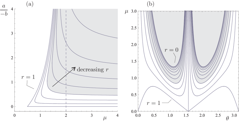
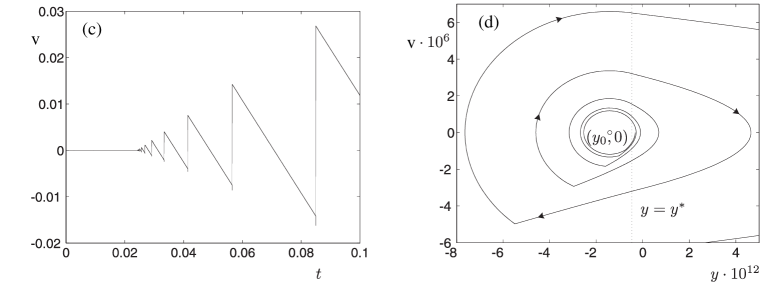
Figure 11: Reproduced from [55], with permission. (a) The region in $a/(-b)$ and $\mu$, for fixed $B=0.5$, $C=A=1$ and various $r$-values, for which $e>1$. The region for which reverse chatter is possible is to the right of the curve depicted for each $r$-value. The case $r=0.7$ leads to the shaded region. Note in this case that the Painlevé region $p^{+}<0$ is given by $\mu>2$. (b) The same plot for the specific case of the CPP (1) in terms of the angle $\theta$. Here the region above each curve for fixed $r$ represents where there exists a range of $\dot{\theta}$-values for which reverse chatter is possible. (c),(d) Simulation of a reverse chatter event in the equations for a falling rod with applied body forces, using a stiff compliant model in which the penetration $y$ is allowed to be violated as in (30), see [55] for the details.

The paper [55] enumerates carefully the cases for which reverse chatter is possible; the results are summarised in Fig. 11(a),(b). Note that it is not a necessary condition that we are in the Painlevé region. In particular, panel (b) illustrates the conditions for $e>1$ for the CPP, and here reverse chatter can be triggered all the way down to $\mu=0$ in the case of perfectly elastic collisions $r=1$.

3.4 Stability

Most forms of motion within rigid-body systems with contact can be described by special solutions (e.g. equilibria, limit cycles or invariant sets) of an appropriately defined dynamical system. In order to understand which of these motions may be observed in practice, it is common to examine the stability of these solutions. There are however several notions of stability in dynamical systems, and the choice of an appropriate definition is made more subtle by the presence of unilateral constraints. Fundamentally though, to define stability we really need to understand two things; what kind of motion is being considered as being stable, and what kind of perturbations should we be stable against.

The simplest kind of motion is equilibrium. Equilibrium configurations in contact only exist if every contact is in stick. We shall consider the case of multiple contact points in Sec. 6. For the present we shall confine ourselves to configurations with a single point of contact. One characterisation of stability of an equilibrium in stick contact is that the the system should resist small variations of external forces. The difficulty of such a definition is that such forces are not usually considered as states of the system, rather as external inputs or parameters. Qualitative invariance of the state of a dynamical system under changes to inputs or parameters is sometimes referred to as robustness (or roughness) of the system, or more general to structural stability rather than dynamic stability. Stability to changes in external forces is sometimes therefore studied by contact regularisation, in which a (large) finite contact stiffness is introduced, so that a change in force necessarily implies a change in the system state. Contact regularisation in the normal direction forms the subject of Sec. 4 below.

More generally, for systems with rigid contact, we can distinguish between normal stability and tangential stability, depending on whether we allow state perturbations at contact points that have components in the normal direction or not. Normal stability requires stability against the possibility of lift-off or impact, whereas tangential stability presumes that contact is always maintained. The study of the former generally requires normal contact regularisation, whereas tangent stability can be conducted using Filippov theory [20], without the need to introduce extra compliance.

The key question in tangential stability is whether general motion in stick (not just restricted to equilibria) can be unstable to perturbations that would cause slip. This question is considered in [55, Sec. 3] for the 2D single-contact case. It is shown that provided $p^{\pm}>0$ and the contact is in interior of the friction cone, then stick (with $u=0$) represents a stable sliding manifold in the sense of Filippov (see also [15]). Thus, motion in stick in case II(iv) of Table 2 is stable to perturbations with $u\neq 0$ except at the boundary of the friction cone where a straightforward transition into either positive or negative slip occurs (depending on which edge of the friction cone is in question). A more subtle argument needs to be used in the case that stick occurs in one of the Painlevé parameter regions (in cells II(ii),(iii),(v) or (vi)). In [55, Sec. 3] it is shown that if stick is normally stable then a posteriori it can be shown that stick is must also be tangentially stable in the sense of Filippov.

Upon consideration of a larger class of state perturbations than just small variations of external forces, the most widely used notion of stability is that of Lyapunov stability, that any small perturbation should remain bounded. A yet stronger condition is asymptotic stability, namely that such perturbations should also decay exponentially. Equilibria involving frictional systems rarely possess asymptotic stability, because dry friction tends to create continuous equilibrium sets, and perturbations typically push the system to a nearby point within the set [44]. Thus it is natural to discuss Lyapunov stability in the context of rigid-body systems with contact. In the robotics community, the concept of strong stability has been proposed to refer to a case where stick is the only consistent mode with $u=0$ at each contact (see [64] and Sec. 6.4 below for further discussion). Or and Rimon [58] refer to such a property as unambiguity and show that it is a necessary condition for Lyapunov stability of a stick equilibrium. We propose here a generalisation of Or and Rimon’s result to stipulate necessary and sufficient condition for Lyapunov stability for an equilibrium in the presence of any conservative external loads and a single point contact. Specifically, three conditions must be met:

1. The curvatures of the object and the contact surface must ensure a local minimum of the potential energy of external forces along trajectories within stick (the $T$ mode). If this criterion is not met, divergence from the equilibrium with the $T$ mode becomes possible.

2. The equilibrium must be unambiguous in the sense of [58]. Unambiguity ensures that the system may not diverge from the equilibrium state in $F$, $S_{+}$ or $S_{-}$ modes unless it undergoes and impact.

3. Additionally, upon defining the effective restitution coefficient $e$ for chatter as in (29), then we must have $e<1$. Otherwise a small perturbation may trigger diverging reverse-chatter motion.

Analogous conditions in the multi-contact case will be discussed in Sec. 6.4

4 Resolution of paradoxes via contact regularisation

Returning to Table 2, we can see that Question 1 can be resolved in the inconsistent regions by the requirement that an IWC must occur. This leaves the indeterminate regions. We shall now analyse these cases in the sense of Question 3, by adopting contact regularisation, that is, introduction of a form of finite elasticity into the model and then passing to the limit that the stiffness tends to infinity. There are a number of different choices that can be made. For example, Neimark and Smirnova [52] propose including both normal and tangential compliance. However, as argued in the previous section, unlike normal stability, tangential stability can be analysed without the need to introduce compliance. Therefore the simplest approach, adopted here, is to introduce compliance in the normal direction only, and otherwise assume that the assumptions of rigid body mechanics occur, including Coulomb friction. A good general discussion of normal compliance can be found in the book by Anh [4].

It is useful though to point out a promising alternative approach due to Szalai [82, 81], who introduced a formulation that models the response of a compliant surface through a delay kernel. In unpublished work, Berdeni [7] applies this approach to the Painlevé paradox. By taking the fast wavespeed limit, a regularisation occurs via additional continuous degrees of freedom for the normal and tangential forces.

Following Nordmark et al [55], we replace the rigid constraint $y\geq 0$ by an assumption that there can be small $O(\epsilon)$ excursions into $y<0$, where $\epsilon>0$ is a small parameter. Furthermore, we suppose that the normal force is given by a specific expression

$$\lambda_{N}(\tilde{y},\tilde{v})=\begin{cases}0&\text{for }\tilde{y}\geq 0,\>\tilde{v}\geq 0\>,\\ f_{N}(\tilde{y},\tilde{v})&\text{otherwise},\end{cases}$$ (30)

where $\tilde{y}=\epsilon^{-1}y$; $\tilde{v}=d\tilde{y}/d\tilde{t}$; $\tilde{t}=\epsilon^{-1/2}t$. Note that the timescale associated with contact is $O(\epsilon^{1/2})$, which explains the scaling of variables. We suppose that the restoring force has the following properties:

1. $f_{N}$ is continuous and $f_{N}(0,0)=0$ so that $\lambda_{N}$ is also continuous, and $f_{N}\to 0$ as $\tilde{y}\to+\infty$

2. $f_{N}$ is also smooth (at least of class $C^{1}$) whenever $f_{N}>0$,

3. $f_{N}$ is restoring, that is

   $$\frac{\partial f_{N}}{\partial\tilde{y}}<0\quad\mbox{for}\quad f_{N}>0,$$

4. $f_{N}$ is dissipative

   $$\frac{\partial f_{N}}{\partial\tilde{v}}<0\quad\mbox{for}\quad f_{N}>0.$$

Such assumptions are essentially equivalent to replacing the normal rigid contact with a (possibly nonlinear) spring and damper in parallel that reach the rigid limit as $\epsilon\to 0$. Moreover, it is also possible to choose the specific function $f_{N}$ such that it relaxes to a (Poisson or energetic) impact law as $\epsilon\to 0$.

4.1 Normal stability of free fall

The free fall mode does not involve active contacts, i.e. $\lambda_{N}=\lambda_{T}=0$. The fact that the contact forces are zero makes them robust against small perturbations. That is if $y>0$ then small perturbations in normal force cannot affect the motion. Alternatively, free motion can occur if $y=0$ and $\dot{v}>0$. Here small perturbation of normal force will not be sufficient to make $\dot{v}=0$. Hence the system remains in $F$ mode in response to small perturbation, which means that we can consider the $F$ mode to be normally stable.

4.2 Normal stability of stick

Introducing the definition (30) into the formulation (8), (9) and assuming the conditions for stick apply, then we have an equilibrium solution in the $y$-direction for which, according to (4.2),

$$\lambda_{N}=\lambda_{N}^{0}=\frac{aB-Ab}{AC-B^{2}}>0$$

and hence we have an equilibrium penetration $\tilde{y}_{0}<0$ corresponding to stick. Now let

$$\tilde{y}=\tilde{y}_{0}+\hat{y},\qquad\lambda_{N}=\lambda^{0}_{N}+\hat{\lambda}_{N}:=f_{N}(\tilde{y}_{0},0)+k\hat{y}+q\tilde{v}+o(\hat{y},\tilde{v}),$$

where

$$k=\left.\frac{\partial f_{N}}{\partial\tilde{y}}\right|_{(\tilde{y}_{0},0)}\qquad q=\left.\frac{\partial f_{N}}{\partial\tilde{v}}\right|_{(\tilde{y}_{0},0)}.$$

are well defined, by property 3 above. Substituting these expressions into (8) and (9), to leading order we obtain

$$\frac{d}{d\tilde{t}}\left[\begin{array}[]{c}\hat{y}\\ \tilde{v}\end{array}\right]=\left[\begin{array}[]{cc}0&1\\ Kk&Kq\end{array}\right]\left[\begin{array}[]{c}\hat{y}\\ \tilde{v}\end{array}\right],$$

where

$$K=\frac{aB-Ab}{AC-B^{2}}>0.$$

Note, from properties 1 to 4 above, that $k<0$ and $q<0$. Hence the $2\times 2$ matrix has two eigenvalues with negative real part. We conclude that the equilibrium $\tilde{y}=y_{0}$ is normally stable. Taking the limit $\epsilon\to 0$, we conclude that stick is normally stable. Note that although $y_{0}\to 0$ in this limit, the normal force $\lambda^{0}_{N}$ remains finite. So in force space, the $T$ mode is not close to the $F$ mode and so stick remains stable against small perturbations. However, the asymptotic stability occurs on the fast time-scale $\tilde{t}$ and so as we pass to the limit $\epsilon\to 0$, the normal Lyapunov exponent tends to $-\infty$.

Thus, upon the introduction of compliance and taking the infinite stiffness limit, a firm conclusion can be made within cells II(ii) and II(iii) of Table 2. That is, if a body is in the state of sustained stick, then this motion is stable to small perturbations in forces and the only way to leave sticking is by reaching the boundary of the friction cone. In particular, a body that is in contact and sticking will remain in stick, even if the Painlevé region with $b>0$ is reached, provided that the body remains inside the friction cone.

4.3 Normal stability of slip

Without loss of generality, consider positive slip. Proceeding similarly to above, we end up with an equation for the normal dynamics that reads

$$\frac{d}{d\tilde{t}}\left[\begin{array}[]{c}\hat{y}\\ \tilde{v}\end{array}\right]=\left[\begin{array}[]{cc}0&1\\ p^{+}k&p^{+}q\end{array}\right]\left[\begin{array}[]{c}\hat{y}\\ \tilde{v}\end{array}\right],$$

where $k,q<0$. Hence there are two eigenvalues with negative real part if $p^{+}>0$ and two real eigenvalues of opposite sign if $p^{+}<0$. Thus we conclude that the normal stability of the equilibrium in the fast-scale dynamics is determined by the sign of $p^{+}$ Thus positive slip is stable to perturbations in the normal direction if and only if the appropriate Painlevé parameter $p^{+}$ is positive. Hence forward slip is unstable in the Painlevé region $p^{+}<0$ (cell I(iii) in Table 2). A similar conclusion holds for negative slip in the case $p^{-}<0$ (cell III(iii)).

Thus we have that no configuration can smoothly evolve during slip into the Painlevé region with $b>0$, as this state would be violently unstable, with a normal Liapunov exponent equal to $+\infty$ in the limit $\epsilon\to 0$. That is, it would be like trying to find an initial condition that can make an infinitely heavy pin balance on its point. This essentially provides a unique answer to Question 2. However, there is a sting in the tail, because if a configuration satisfied the conditions to be in such a ‘Painlevé slip’ case at time $t=0$, it must leave, because the state is violently unstable. However, thinking of the compliant limit again with finite $\epsilon$, there are two possibilities. From the unstable equilibrium depth $\tilde{y}_{0}<0$ the body could perhaps “fall” into a state with $f_{N}<f_{N}^{0}$ in which case it must lift off into free motion. However it could also “fall” to the other side, $f_{N}>f_{N}^{0}$, in which case an IWC would occur. After the IWC has terminated, the body would have very different values of tangential and normal velocities than if it had just lifted off. So there remains an indeterminacy, in the sense of Question 1 of the introduction. An indeterminacy that is, not between slip and lift-off but between lift-off and IWC. It becomes imperative therefore to understand how a system can transition into a state of painlevé slip.

4.4 Updated contact mode consistency

	I:   $u>0$	II:   $u=0$	III:   $u<0$
(i): $b>0$, $p^{+}>0$, $p^{-}>0$	$F$	$F$	$F$
(ii): $b>0$, $p^{+}>0$, $p^{-}<0$	$F$	$F$ or ($F$ and $T$)	$F$ and IWC
(iii): $b>0$, $p^{+}<0$, $p^{-}>0$	$F$ and IWC	$F$ or ($F$ and $T$)	$F$
(iv): $b<0$, $p^{+}>0$, $p^{-}>0$	$S_{+}$	$T$ or $S_{+}$ or $S_{-}$	$S_{-}$
(v): $b<0$, $p^{+}>0$, $p^{-}<0$	$S_{+}$	$S_{+}$ or $T$	IWC
(vi): $b<0$, $p^{+}<0$, $p^{-}>0$	IWC	$S_{-}$ or $T$	$S_{-}$

Table 3: Updated version of Table 2, taking into account the results of Secs. 3 and 4.

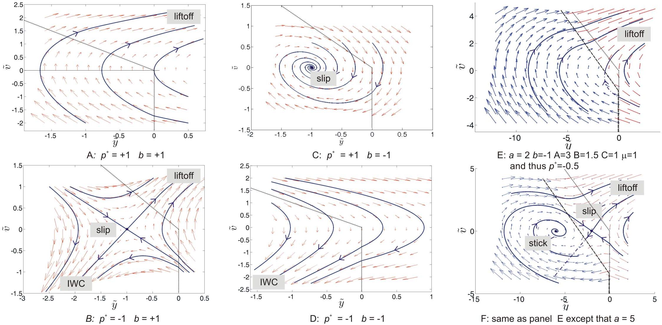
Figure 12: Phase portraits of fast contact dynamics of a point contact with $k=q=-1$. Panels A–D illustrate cases for $u>0$, specifically A: case I(i-ii) of Table 3, B: case I(iii), C: case I(iv-v) and D: case I(vi) (panel D) of Table 3. Panels E and F show two different phase portraits for zero initial tangential velocity $u=0$, in case II(ii). E shows the case where lift-off always occurs, whereas F illustrates the case of indeterminacy between $F$ and IWC. Dotted lines in all panels show the border between active ($f_{N}>0$) and passive ($f_{N}=0$) contacts. The dashed line in panels E and F depicts states for which the contact force is at the boundary of the friction cone. To the right of this line, there is positive tangential acceleration at the contact point.

In the light of the above analysis, we can update Table 2, to take account of the normal stability results and the possibility of impact; see Table 3. The above-mentioned indeterminacy between lift-off and impact occurs in cells III(ii) and I(iii). There is also another indeterminacy in cells II(ii) and II(iii) where either stick or lift off can occur, which we shall explain shortly.

To understand either of these indeterminancies though it is useful to illustrate phase portraits of the regularised contact dynamics. See Fig. 12, in which we have used (30) with

$$f_{N}=\max\left[\begin{array}[]{c}k\tilde{y}+q\tilde{v}\\ 0\end{array}\right]$$ (31)

where $k$ and $q$ are negative scalars.

Consider first cases where the initial condition is in slip and, without loss of generality, let us assume $u>0$. The four possible cases are illustrated in Fig. 12(A-D). If $b<0<p^{+}$ (case I(iv)) then the normal dynamics has a globally attractive equilibrium corresponding to positive slip. In contrast, if $b>0>p^{+}$ (case I(iii)) the positive slip normal equilibrium corresponds to a saddle point, and trajectories converge to $\tilde{y}=+\infty$ (liftoff) or $\tilde{y}=-\infty$ (IWC) depending on initial conditions. In the remaining two cases, slipping was found inconsistent in Sec. 3. Accordingly the dynamics of the compliant contacts has no equilibrium and every trajectory converges to $\tilde{y}=+\infty$ if $0<b,p^{+}$, or to $\tilde{y}=-\infty$ if $0>b,p^{+}$. This picture confirms the result that the contact undergoes liftoff in case I(i) and IWC in case I(iv).

Consider now initial conditions for which $u=0$. Then in all cases other than II(ii-iii), phase portraits like Fig. 12(A) or (C) occur where now the normal equilibrium corresponds to stick rather than slip if the equilibrium is in the interior of the friction cone. Fig. 12(E) and (F) illustrate the possibly indeterminate case II(iii) (case II(ii) is similar). Panel E represents the case where the configuration (ignoring normal compliance) is outside of the friction cone and the only possibility is motion in $F$ mode. Here a dashed line shows those states for which zero tangential acceleration requires $\lambda_{T}=-\mu\lambda_{N}$. To the left of this line, the contact remains in stick, whereas to the right of this line it has positive tangential acceleration so that slip or lift-off must occur. Crossing from left to right corresponds to a stick-slip transition, whereas crossing from right to left does not represent a transition because $u>0$. These latter trajectories do not follow the depicted (sticking) vector field as long as the tangential velocity of the contact point remains positive; one such trajectory is depicted by a dot-dashed line. Nevertheless we see in this case that all initial conditions eventually lead to lift-off, and so $F$ remains the only mode.

Fig. 12(F) illustrates the other branch of the “or” in cell II(iii) of Table 2 in which there are additional feasible $T$ and $S_{+}$ modes. Here we see that the $T$ mode represents a stable focus whereas slipping $S_{+}$ can be seen to be a saddle point, and hence unstable, in accordance with the calculations in Secs.  4.2 and 3.3 above. Note though that there is still indeterminacy in this case, because lift off (mode $F$) is another possibility, which is represented here by trajectories diverging to positive infinity in $y$. Note that the stable manifold of the saddle separates trajectories that are attracted to mode $T$ from those which lift-off.

5 Triggered transitions between states

In this section we focus on Question 2, namely what are the generic ways in which a configuration can enter a Painlevé region and what must then happen. Theoretically, there are only two ways of reaching sustained contact in a Painlevé state; (1) moving from non-Painlevé contact to Painlevé contact, or (2) establishing sustained contact via the termination of a chattering sequence, inside the Painlevé regime. We deal with these two possibilities in the next two subsections. We shall then look at ways in which reverse chatter may be triggered while in contact.

5.1 Entering a Painlevé region within contact; the G-spot

Suppose at some time $t_{0}$ that a rigid-body system is contact with both $p^{\pm}>0$. We want to know how to continue the dynamics for $t>t_{0}$. Note that parameters $p^{\pm}$, $a$ and $b$ will be smooth functions of time provided the body doesn’t change its mode of motion (between stick, slip or free motion). The analysis in the previous section shows that any body in stick should remain in stick provided it remains in the friction cone. In particular a change of sign of $p^{\pm}$ would not affect the mode of motion. This is not true of slip though. As we have seen, if the appropriate Painlevé parameter becomes negative, then slip changes from being highly stable to highly unstable.

For definiteness let us consider a positive slip $u>0$ within region I(iv) of Table 3; the analysis for negative slip is similar. We are interested in where $p^{+}$ being close to zero for $b<0$. So suppose we have an initial condition with $0<p^{+}\ll 1$. Hence, according to (15) the contact force $\lambda_{N}$ is large. In particular, we can see that if $p^{+}\to 0$ while $b$ remained finite, then $\lambda_{N}\to+\infty$ which implies $\lambda_{T}=-\mu\lambda_{N}\to-\infty$. Large contact force means large accelerations. When viewed in state space, we find that these large accelerations must cause motion in the direction tangent to the boundary $p^{+}=0$, and so the boundary cannot be crossed transversely.

In the case of systems with three degrees-of-freedom like the CPP, and any system composed of a single rigid body with a unique point contact, then the set $p^{+}=0$ is a 1-dimensional sub-manifold of the set of slipping trajectories. A more precise analysis can be performed by realising that the above arguments show the dynamics of slip becomes singular as $p^{+}\to 0$ and rescaling time appropriately. Following Génot and Brogliato [22] it then can be shown that $p^{+}=0$ is composed of a solution trajectory in this rescaled time. Thus, there can be no crossing into the Painlevé region except possibly at a singular point of the rescaled slipping vector field. The only such singular point of in this case is where $b=p^{+}=0$.

The analysis in [22] was specific to the CPP; we sketch here a generalisation of what must occur for any system close to the so-called G-spot, $b=p=0$, a complete version of which will appear elsewhere [54]. The trick in [22] is to analysis the problem by rescaling time

$$dt=p^{+}ds,$$ (32)

and then to think of the scalar variables $p^{+}$ and $b$ as dynamical quantities that evolve on the timescale $s$. From (8), (9) we then obtain, to leading order in $p^{+}$ and $b$,

$$\frac{d}{ds}p^{+} = \alpha_{1}p^{+},$$ (33)

$$\frac{d}{ds}b = \alpha_{2}p^{+}+\alpha_{3}b,$$ (34)

where

$$\alpha_{1} = \dot{q}\cdot\frac{\partial}{\partial q}p^{+}+\frac{\partial}{\partial t}p^{+},$$

$$\alpha_{2} = M^{-1}f\frac{\partial b}{\partial\dot{q}}+\frac{\partial b}{\partial q}\dot{q}+\frac{\partial b}{\partial t},$$

$$\alpha_{3} = M^{-1}\left(\mu c-d\right)\frac{\partial b}{\partial\dot{q}}.$$

Here all functions are evaluated at the codimension-two point where $p^{+}=b=0$, in which case $\alpha_{1--3}$ are just real constants. Specifically $\alpha_{1}$ is just the time derivative of $p^{+}$ and $\alpha_{2}$ the time derivative of $b$, whereas $\alpha_{3}$ is the time derivative of the dependence of $b$ on the parameter $p$.

As an example consider the CPP for a uniform rod with $m=1$, $l=2$. Then

$$\alpha_{1} = -3\omega\left(\sin 2\theta+\mu\cos 2\theta\right)$$

$$\alpha_{2} = 9R\omega\sin\theta+\omega^{3}\cos\theta+\dot{S}_{y}-3\dot{R}\cos(\theta)$$

$$\alpha_{3} = -6\omega\sin\theta\left(\mu\sin\theta-\cos\theta\right),$$

where $S_{y}$ and $R$ are the $y$-component of torque component of body forces at the centre of mass. Note that for general configurations, such as those reviewed in Sec. 2, the $\alpha$ parameters can take any combination of signs.

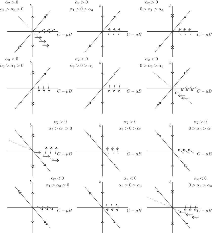
Figure 13: Reproduced from [54]. Analysis of the dynamics of the neighbourhood of the G-spot. In each panel, the phase plane of (33), (34) is depicted, for all possible sign combinations of the parameters $\alpha_{1,2,3}$. Here the bold line passing through the origin represents the location of the second eigenvector, and the arrows on this line and the $b$-axis represent whether each represents a stable or unstable manifold. In the case of a two-dimensional stable (unstable) eigenspace, double arrows are used to represent the strong stable (unstable) manifold. The dashed line represents the location of the horizontal nullcline. Arrows crossing this line and also the $(C-\mu B)$-axis indicate the direction of solution trajectories there

Note that in the rescaled singular timescale $s$, the G-spot is an equilibrium point and the dynamical system (33), (34) provides a planar linear system whose dynamics govern the behaviour near this singular equilibrium. Note that the singularity of the time rescaling at the G-spot means that the system (33) (34) only makes sense in the original co-ordinates if $p^{+}\neq 0$.

Figure 13 shows all possible qualitatively distinct phase portraits close to the G-spot. We are interested in what happens to initial conditions that are initially in slip, that is in the bottom right quadrant $p^{+}>0$, $b<0$. To explain the figure, note that the coefficient matrix

$$\begin{pmatrix}\alpha_{1}&0\\ \alpha_{2}&\alpha_{3}\end{pmatrix}$$

has two eigenvalues $\alpha_{1}$ and $\alpha_{3}$ with eigenvectors $(\alpha_{1}-\alpha_{3},\alpha_{2})^{T}$ and $(0,1)^{T}$, respectively. In particular, since it always corresponds to an eigenvector, independently of the value the coefficients $\alpha_{1,2,3}$, the $b^{+}$ axis is invariant. This latter fact shows immediately that an initial condition with $p^{+}>0$, $b<0$, cannot evolve into the Painlevé region $p^{+}<0$ except possibly at the G-spot $p^{+}=b=0$. In fact Fig. 13 shows that there are only three possible outcomes for any open set of initial conditions starting in the bottom right quadrant:

1. lift off via passage through $b=0$ for $p^{+}>0$,

2. continued slip by moving away from a neighbourhood of the origin while remaining in the bottom right quadrant,

3. approaching the G-spot.

The first two possibilities are regular transitions that do not involve the singularity $p^{+}\to 0$. Possibility 3 is rather special though, and although the G-spot is an isolated codimension-two point in phase space, it can attract an open set of initial conditions, owing to the fact that it is an equilibrium point in the rescaled dynamics.

Note that this third possibility can only occur in panels (c), (e) and (i) of Fig. 13, which really split into two separate cases. Either convergence to the G-spot is tangent to the $b$ axis, or it is tangent to the $\alpha_{1}$-eigenvector that is the line $\alpha_{2}p^{+}=(\alpha_{1}-\alpha_{3})b$. Note in the former case we have that $\lambda_{N}=-b/p^{+}$ becomes infinite, as we approach the G-spot, whereas in the former case $\lambda_{N}$ tends to the finite limit associated with the non-trivial eigenvector. Recalling that in the unscaled time, the G-spot is reached in finite time, we thus have two possibilities:

G1

If $0>\alpha_{3}>\alpha_{1}$ and the initial condition $(p^{+},b)$ in the lower right quadrant close to the G-spot is such that $\alpha_{2}p^{+}<(\alpha_{1}-\alpha_{3})b$, then the G-spot is approached in finite time such that ratio $p^{+}/b\to 0$ and the normal force $\lambda_{N}\to\infty$.

G2

If $\alpha_{2}<0$, $0<\alpha_{1}<\alpha_{3}$ then the G-spot is approached in finite time, and $\lambda_{N}$ approaches the finite limit $\alpha_{2}/(\alpha_{3}-\alpha_{1})>0$.

Each of these cases correspond to what has been referred to in the literature as dynamic jam. What happens next beyond dynamic jam remains an open question. In principle after the G-spot, there could be an IWC, a lift off event or even possibly a velocity jump immediately into stick (recall that $u>0$ as we approach the G-spot). It seems that these possibilities cannot easily be distinguished using the contact regularisation approach of Sec. 4.

5.2 Reaching a Painlevé state via complete chatter

The analysis in Secs. 3 and 4 analyse both stick and slip in the Painlevé regions, assuming that a trajectory arrived in the Painlevé state by smooth evolution while in contact. We found that stick is unaffected by either $p^{\pm}<0$, provided the body is in the interior of the friction cone. In contrast, the analysis in Sec. 5.1 above shows that the only way to enter the Painlevé region while slipping is via the G-spot. What we have not investigated though is whether a complete chatter sequence can end up a Zeno point that is in the Painlevé region.

In order for a chattering sequence to occur, we must have $b<0$. Hence the indeterminate cases of stick (cells II(ii) and III(ii) in Table 3) cannot be reached. So, consider instead the possibility of slip. Suppose that the parameter $p^{+}<0$ and consider the possibility of a chattering sequence leading to positive slip. Here, we are in the case of impact mappings as depicted in Fig. 10(b). Note that any impact with an initial velocity with $u^{-}>0$, must end up with $u^{+}=0$. Similarly any impact with $u^{-}<0$ ends up with $u^{+}\leq 0$. Hence the only possibility is that the Zeno point has $u\leq 0$. But note that there is no inconsistency or indeterminacy in this case (see cells I(vi) and II(vi) in Table 3). We either get stick or negative slip, the latter of which is consistent because $p^{-}>0$.

A similar conclusion holds if $p^{-}<0$, we cannot approach the Painlevé region for negative slip as the result of a chattering sequence. We conclude that even if one of the parameters $p^{\pm}<0$, it is not possible to have a Zeno point in the Painlevé region, thus dismissing this is a possible route into the Painlevé region.

5.3 Triggering reverse chatter

A final possibility for a complex triggered transition would be if a body that is smoothly in contact, were to spontaneously undergo a reverse chatter sequence. This possibility was considered by Nordmark et al [55], the results of which we summarise here.

In general, we can rule out such a spontaneous triggering of reverese chatter in T mode by the analysis of Sec. 4.2 since, provided the body remains in the interior of the friction cone, stick is stable. Similarly, the analysis of Sec. 4.3 rules out the possibility of spontaneous triggering of reverse chatter from within a condition of sustained slip, as this is stable wherever it is consistent (unless the border of Painlevé-ness is crossed, which was shown to be impossible). Similarly, reverse chatter cannot be triggered at the end of a forward chattering sequence, because such a sequence necessarily converges to a point where $e<1$.

This leaves the possibility that reverse chatter can be triggered at the boundary of one of the contact phases, namely at the termination of stick, or of slip. But, an analysis of the cases where $e$ can be greater than one shows that these are necessarily a subset of the cases that are in the interior of the friction cone. Hence it can be concluded that reverse chatter can only be triggered at the end of a slip phase. Then, it can be argued that either a case of stick is triggered, or under certain other conditions, in addition to $e>1$, we might get the triggering of reverse chatter.

Nordmark et al [55] enumerate the details and find that there are further inequality conditions on $a$, $b$, $A$, $B$, $C$, $\mu$ and $r$ that determine whether reverse chatter can be triggered from a transition into stick. Then they show, by introducing a compliant model, as in Sec. 4, that if these conditions are satisfied then the situation is not uniformly resolvable. That is, the precise details of the compliant force $f_{N}$ can affect whether regular stick motion of reverse chatter is triggered. We are left with another indeterminate case.

6 Multiple contact points

Let us now consider generalisation of the previous results to systems with multiple contacts. One aim is to identify which properties of Painlevé’s paradox are generally true, and which are specific properties of single-contact systems. Moreover, we will uncover many extra forms of degeneracy that are unique to multiple-contact point systems.

One of the main difficulties with answering Question 1 is that if we allow $F$, $T$, $S_{+}$ and $S_{-}$ at each of $n$ contacts, then this induces $4^{n}$ possible contact modes (although some of them will be kinematically inadmissible). This combinatorial complexity makes a consistency check for each potential combination computationally unfeasible for large $n$. In what follows we therefore focus mostly on the simplest case of just two frictional contacts.

Ivanov [32] considered generalisations of the CPP for a rod that has two points of contacts with rough rigid surfaces under the assumption that each contact undergoes slip. He enumerated the conditions under which the Painlevé paradox appears for suitably chosen external forces. The classification scheme of Ivanov has recently been refined by Várkonyi [84] to the level of our analysis in Sec. 3.1. A summary of and commentary on these results appear in the next three subsections.

6.1 Consistency analysis of contact modes

To begin with, consider a planar rigid-body system that has two point contacts, with nonzero tangential velocities: $x_{i}=y_{i}=v_{i}=0$ and $u_{i}>0$ for $i=1,2$. Thus there are four kinematically admissible modes: $S_{+}S_{+}$, $S_{+}F$, $FS_{+}$, and $FF$. Here the two-letter symbols refer to the specific combination of modes at the two contacts. The contact forces and accelerations are determined with the help of the equality constraints of Table 2 for both contacts. A contact mode is deemed consistent, if the consistency conditions of Table 2 are satisfied for both contacts.

The key observation is that the general analytical expressions for contact motion in Sec. 3 still apply, specifically the equation (14), but where now $b$ and $\lambda_{N}$ are vectors in ${\mathbb{R}}^{2}$ and $p^{+}$ is a matrix of size $2\times 2$. In this formulation, the elements $p^{+}_{ij}$ of $p^{+}$ represent the normal acceleration of contact $i$ in response to a slipping contact force with a normal component of unit size at contact $j$.

Várkonyi [84] has recently enumerated all the consistent modes under this restriction of no sticking modes. In order to summarise the results of his analysis, it is convenient to introduce the following notation. Let $p_{j}$ represent the $j^{th}$ column vector of $p^{+}$ such that $p^{+}=[p_{1}\;p_{2}]$. Furthermore, let $\gamma_{j}$ be the angle between $p_{j}$ and vector $[1\;0]^{T}$. For example, if $p_{j}=[0\;1]^{T}$ then $\gamma_{j}=\pi/2$. Similarly, we let $\hat{\gamma}_{j}$ be the angle between $-p_{j}$ and the vector $[1\;0]^{T}$ and $\beta$ be the angle between $-b$ and $[1\;0]^{T}$. It can be shown that the consistency of each contact mode can be determined using a string of three integers

$$s_{1}s_{2}s_{3},\quad\mbox{where}\quad s_{1}\in\{1,2,3,4\},\quad s_{2,3}\in\{1,2,\ldots 6\},$$

which code the relative position of the vectors $p_{1}$, $p_{2}$, $b$ and the co-ordinate axes. Specifically the index $s_{1}$ represents the quadrant of ${\mathbb{R}}^{2}$ that contains $p_{1}$. Equivalently, $s_{1}$ is the index of the interval among the four ordered intervals $[0,\pi/2]$, $[\pi/2,\pi]$, $[\pi,3\pi/2]$, $[3\pi/2,2\pi]$ that contains $\gamma_{1}$. In a similar fashion, the second integer $s_{2}$ represents the index of the interval among the set of ordered closed intervals bounded by $0$, $\hat{\gamma_{1}}$, $\gamma_{1}$ $\pi/2$, $\pi$, $3\pi/2$ and $2\pi$ that contains $\gamma_{2}$. The final integer $s_{3}$ represents the index of the interval among the set of ordered closed intervals bounded by $0$, $\gamma_{1}$, $\gamma_{2}$ $\pi/2$, $\pi$ $3\pi/2$ and $2\pi$ that contains $\beta$.

The relative positions of the vectors $p_{1}$, $p_{2}$ and $b$ corresponding to each class of configurations is depicted in Fig. 14. Thus, for example, the upper right panel refers to classes 14$s_{3}$ where $s_{3}=1,2,3\ldots 6$. Here we see, according to the above notation, that $s_{1}=1$ and so $p_{1}$ is in the first quadrant. In addition, $s_{2}=4$ and so $p_{2}$ is in third quadrant with positive angle to the $[0\;1]^{T}$ axis that is less than that of $-p_{1}$. The $s_{3}$-value corresponding to possible locations of $b$ are indicated by dashed arrows, which depicts the relative position of the vector $b$ with respect to $p_{1}$, $p_{2}$ and the four co-ordinate semi-axes.

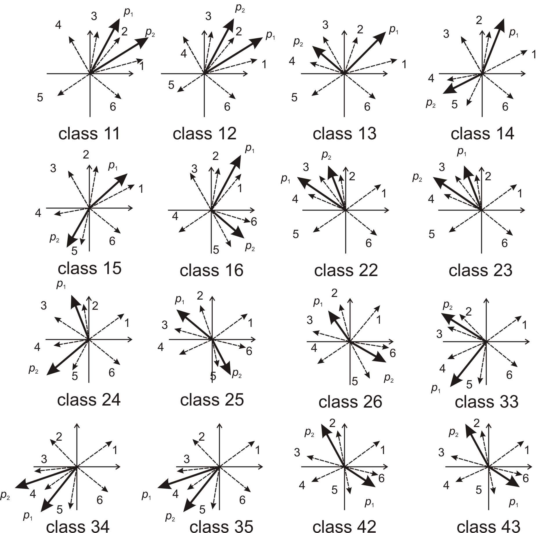
Figure 14: Relative positions of the vectors $p_{1}$ and $p_{2}$ (solid arrows) and the four co-ordinate semi-axes in each class $s_{1}s_{2}$. In each case, every possible position of the third vector $b$, which delineates the third integer $s_{3}$ is indicated by a dashed arrow. Note that only one member of each dual pair of classes is displayed, see Table 4 for the corresponding dual $\hat{s}_{1}\hat{s}_{1}$ in each case.

Classes	Contact modes				IWC
name (dual)	$FF$	$S_{+}S_{+}$	$S_{+}F$	$FS_{+}$	$IF$	$FI$	$II$
11 (self)	5	2	1 2 6	2 3 4
12 (self)	5	2	1 6	3 4
13 (41)	5	2 3	1 6	4
14 (31)	4 5	2 3 4	1 6	4			(x)
15 (32)	4 5	1 5 6	1 6	4			(x)
16 (21)	4	1 6	1 5 6	4 5		x
22 (45)	5	3	4 5	3 4	x
23 (46)	5	3	3 4 5	4	x
24 (36)	4 5	3 4	3 4 5	4	x		(x)
25 (self)	4	3 4 5	3 4	4 5	x	x	(x)
26 (self)	4	1 2 6	3 4	4 5	x	x
33 (44)	4 5	3 4	5	3			(x)
34 (self)	3 4 5	4	5	3			(x)
35 (self)	3 4 5	4	4 5	3 4			(x)
42 (self)	4	1 2 6	5	3
43 (self)	4	3 4 5	5	3			(x)

Table 4: Classification of planar systems with two non-sticking contacts. See text for details.

The results of the consistency analysis are summarised in Table 4. To cut down the number of rows of the table and sub-panels of Fig. 14, we have used the fact that each class has a dual that is obtained by swapping the labels of contact 1 and contact 2. This corresponds to swapping the labels $p_{1}$ and $p_{2}$ and reflecting both vectors in the line $45^{\circ}$ line in each case. The dual class $\hat{s}_{1}\hat{s}_{2}$ of each of the depicted cases $s_{1}s_{2}$ is given in brackets in the first column of Table 4, including cases that are self-dual. Note that the first two digits $s_{1}s_{2}$ of any class represents the coarser classification of Ivanov [32]. The last digit $s_{3}$ refines the classification into subclasses within which the consistency of each contact mode becomes uniquely determined (as depicted in columns 2 to 5 of the table). The significance of the shading of these columns and the meaning of the last three columns will be explained in the next subsection.

Note already that there are multiple occurrences of indeterminacy and inconsistency indicated in the table. For example, within class 15, subclasses 151, 154 and 156 are indeterminate because two contact modes in each case are consistent. In contrast subclasses 152 and 153 are inconsistent because there is no consistent contact mode for these cases. There are also several examples of triple indeterminacy, for example in subclass 112 where $S_{+}S_{+}$ and $S_{+}F$ and $FS_{+}$ are all consistent and of quadruple indeterminacy where all four possible contact modes are consistent, for example in subclasses 254 or 354.

Before going on to look at normal stability of these modes and the possibility of impact, it is worth stressing that Table 4 is only a partial classification for two contacts, because it ignores stick and cases where negative and positive slip can simulateously occur at different contacts. As far as the authors know, a general classification is not yet known, nor is a classification in cases where there are more than two contacts. Nevertheless, other examples of indeterminacy are known. Two such cases were illustrated in Fig. 7. The left-hand panel depicts a case in which the static equilibrium represents the $TT$ mode which is consistent provided there is a sufficiently large friction force at the contacts (solid arrows in the figure show the gravitational force and a possible choice of reaction forces). Simultaneously, the $FF$ mode is also consistent, in which case the block will just fall. The right-hand panel of Fig. 7 illustrates a shape resting on a slope in which both the body may be in equilibrium in mode $TT$, but for which motion in mode $S_{+}F$ is also consistent.

6.2 Contact regularisation and stability analysis

To resolve the indeterminate cases, we can compute the normal stability of different kinds of contact via the method introduced in Sec. 4. That is, we introduce a contact regularisation in the normal direction, linearise the ensuing equations of motion, perform an eigenvalue analysis on the appropriate Jacobian matrix and then pass to the infinite stiffness limit.

Applying this methodology to the cases enumerated in Table 4, it is straightforward to see that a contact in mode $F$ does not influence the normal stability. Hence, the stability analysis of the $S_{+}F$ and $FS_{+}$ contact modes is identical to the analysis of $S_{+}$ in Sec. 4. Specifically, we obtain that $S_{+}F$ is stable if $p_{11}>0$ and $FS_{+}$ is stable if $p_{22}>0$. For the $S_{+}S_{+}$ mode, the simultaneous dynamics of two contacts is described by a system of four first-order ODEs, and thus normal stability analysis requires the study of eigenvalues of a $4\times 4$ Jacobian matrix. The Jacobian and thus the stability properties of contact modes are independent of $b$. Hence the same results are obtained for all subclasses within this class.

The results of the stability analysis are summarised in Table 4. Details of the calculations are presented in [84]. Stability information is indicated by shading of the appropriate cell in the table. A dark (grey) shading indicates definitely unstable. Lighter (yellow, colour online) shading represents where the $S_{+}S_{+}$ mode may be stable, depending on further conditions. Finally, no shading represents a normally stable situation. One interesting thing to note is that the stability of the $S_{+}S_{+}$ mode is not uniquely determined in classes 13, 41, 14, 31, 23 and 46. The unstable regions within these subclasses are caused by so-called mode coupling – a phenomenon studied in the context of break squeal (see e.g. [30, 27]). In these regions, a system may cross the stability boundary during its motion. In such a situation, a spontaneous contact mode transition will occur. That is, the system would switch from the $S_{+}S_{+}$ mode to a different type of motion, despite the fact that the $S_{+}S_{+}$ mode remains consistent. As we argued in Secs. 3 and 4 such spontaneous transitions are not possible in the single-contact case.

Another intriguing property of these sometimes unstable $S_{+}S_{+}$ regions is that their exact boundaries within a subclass appear to depend on the underlying compliant contact model, even if the compliance parameter $\epsilon\to 0$. Hence, unlike in the single-contact case, the stability of a contact mode may be undecidable within rigid-body theory.

A closer look at Table 4 reveals an even more surprising phenomenon. In subclasses 261 and 262, the $S_{+}S_{+}$ is the unique consistent contact mode. These cases appear to be free from any paradoxes, but nevertheless the stability analysis shows that the $S_{+}S_{+}$ mode is robustly unstable. Robustness is meant in the sense of uniform resolvability, as introduced within Question 3 in the Introduction. That is, instability emerges as $\epsilon\to 0$ for any form of contact compliance within the framework of Sec. 3.2. As we shall see in the next subsection (see e.g. Fig. 15(A)), an IWC is likely to happen in these cases.

This observation refutes an often assumed hypothesis within the rigid body mechanics community that the failure of an object to slip smoothly along contact surfaces is always a result of the Painlevé paradox. This philosophy is embodied in an a priori rule known as Kilmister’s principle of constraints [10]: ”a unilateral constraint must be verified with (bounded) forces each time it is possible, and with impulses if and only if it is not possible with forces”. The observation also questions the relevance of enumerating every possible consistent contact modes, which is often assumed in a hybrid systems or complementarity formation to be the key question in the analysis of mechanical systems with frictional contacts, see e.g. [47, 64].

6.3 Impacts without collision

Let us now consider the possibility of impact, specifically an IWC for each of the cases enumerated in Table 4. This is indicated in last three columns of the table using a notation we shall now explain. A system with multiple contacts may undergo several types of impacts: an impulsive contact force may occur at any non-empty subset of the contact points, while the rest of the contacts lift off. In the simplest case of two non-sticking contacts, we have three types of IWC: impulsive force at one contact while the other lifts off, which we label by $IF$ or $FI$ depending on which compact impacts; and simultaneous impact at both contacts, which we label $II$.

Provided that we retain the assumption that the response of the object follows rigid body-theory, the $IF$ impact is consistent if the contact force at contact 1 seeks to push the contact point into the ground and simultaneously seeks to detach the other point. That is we require $p_{11}<0$ and the other point $p_{21}>0$. Analogously, $FI$ may occur only if $p_{22}<0$ and $p_{12}>0$.

The case of the $II$ impact is more subtle. It is a necessary condition that there must exists a combination of positive impulsive contact forces at the two contacts, which accelerates both contact points towards the ground. In other words, the cone spanned by vectors $p_{1}$ and $p_{2}$ should intersect the fourth quadrant of ${\mathbb{R}}^{2}$. Nevertheless, this condition can be shown to not be sufficient. To study the simultaneous dynamics of the two contacts during a double-impact process in general requires a careful analysis using a compliant contact model.

Thus the notation in the final three columns of Table 4 is to indicate with an ‘x’ where impacts of each type are possible. For the case of $II$ impacts, we have indicated by ‘(x)’ where the necessary conditions are satisfied.

The results of what happens in a double impact $II$ can be shown to depend heavily on the exact form of the compliance model (satisfying the properties given in Sec. 4), or equivalently of the impact model. The details will be presented elsewhere [83]. Computations reveal that there exist cases in which every contact mode is either inconsistent or unstable, and simultaneously, the three forms of IWC mentioned above are impossible, see Fig. 15(B). This observation points towards the incorrectness of another common assumption: that Painlevé’s paradox is perfectly resolvable by considering IWCs.

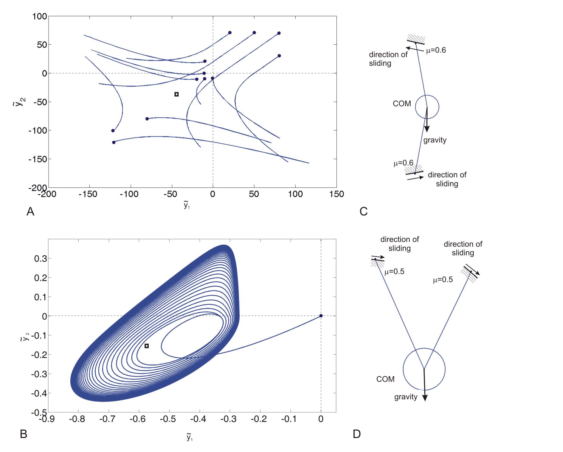
Figure 15: Simulation of fast contact dynamics in examples of (A) class 261 and (B) class 142 using the contact model (31). See text for details. The corresponding panels (C) and (D) show possible configurations that display the dynamics in panels (A) and (B) respectively. Parameter values used are (A) $a=[1\;1]^{T}$, $B=[[-0.055\;0.055]^{T}\;[0.088\;-0.036]^{T}]$, inducing $\gamma_{1}=0.75\pi$; $\gamma_{2}=1.875\pi$; $\alpha=0.25\pi$, and (B) $a=[1\;0.727]^{T}$, $B=[[3.051\;1.555]^{T}\;[-1.677\;-0.0375]^{T}]$, $k_{1}=1$; $k_{2}=3$; $q_{1}=q_{2}=1.2$, inducing $\gamma_{1}=0.15\pi$; $\gamma_{2}=1.07\pi$; and $\alpha=0.2\pi$.

Figure 15(A) shows a planar projection of the phase portrait of the fast contact dynamics for a configuration within class 261 (where the $S_{+}S_{+}$ mode is the unique consistent contact mode, but it is unstable, see Sec. 6.2). Several different initial conditions are depicted in which the initial time derivatives of $\tilde{y}_{i}$ are 0. The contact model (31) is used in the simulation, with $k=q=-1$. For every possible initial condition, one of the two contact penetrations, and hence the normal force diverges to minus infinity. The other contact always lifts off. In the rigid limit $\epsilon\rightarrow 0$ this behaviour corresponds to an IWC at one of the two contacts, and lift off at the other, that is, either mode $IF$ or mode $FI$. Note that the contact dynamics also has a consistent mode $S_{+}S_{+}$ in which both contacts slip, marked by a square in the figure, but this is unstable. The stable manifold of this point in the fast dynamics represents the dividing surface between two different types of IWC.

Figure 15(B) shows an example within class 142 in which there is the onset of some kind of micro-scale sprag-slip oscillation. Here there is also an unstable $S_{+}S_{+}$ mode, again represented by a square. For the parameter values depicted, every other contact mode is inconsistent and IWCs are not possible either. The initial condition for the trajectory depicted is $\tilde{y}_{1}=\tilde{y}_{2}=\dot{\tilde{y}}_{1}=\dot{\tilde{y}}_{2}=0$. The dynamics converges to an attractive limit cycle representing slipping motion accompanied by fast micro-vibration, with repeated liftoff and impact at the second contact point. In the limit $\epsilon\to 0$ this would correspond to a strange kind of sprag-slip limit cycle, for which the period is infinitesimally small.

Panels C and D of Fig. 15 show representations of slipping rigid bodies possessing the values of matrix $B$ that correspond to the cases shown in panels A and B, respectively. The bodies are under the influence of gravity, whose direction is represented by the solid arrow through the centres of mass (COM). The orientation of the vector $b$ for each body, depends on the slip velocity, with the case illustrated corresponding to this velocity being close to zero. The shape and dimension of each body and its point of contact are represented graphically by a circle that shows the radius of gyration centred at the COM, and two solid line sections terminating at the contact points. The orientations of the contact surfaces are represented by bold lines with hatched fills. The values of the coefficient of friction is specified by a label at each contact.

6.4 Stability of equilibria

Stability of equilibrium configurations of rigid-body systems with multiple unilateral contacts is of particular practical importance in robotics, where one needs to be able to demonstrate that grasping manoeuvres are robust. In this context Pang and Trinkle [64] proposed various characterisations of stable equilibrium configurations of systems with any number of contacts. They refer to a configuration as exhibiting the weak stability property if the $TT..T$ mode is consistent and the strong stability property if $TT..T$ mode is the only consistent contact mode which has $u=0$ for all contacts. However, they did not explore the consequences of these notions of “stability” from the point of view of dynamical systems theory. Howard and Kumar [29] demonstrated that the strong stability property of Pang and Trinkle is not necessary for stability against small external forces (structural stability) for the case of a planar rigid body with any number of contacts. An extension of this result to multibody systems was given in [85].

We found in Sec. 3.3 that reverse chattering can occur in a system with a single contact, if $b<0$ and the effective restitution coefficient $e>1$. We also pointed out in Sec. 3.4 the significance of avoiding reverse chatter in proving Lyapunov stability of equilibria. The case of multiple contacts is more complex because a sequence of impacts may include impacts at any of the contact points in regular (periodic) or irregular (chaotic) order. In some cases, simultaneous impacts at multiple points are also to be expected.

Or and Rimon [59] were the first to point out that the key to understanding Lyapunov stability of equilibria with unilateral frictional point contacts is to understand the possibility of reverse chattering motion of the system. They developed a sufficient condition for Lyapunov stability of a planar rigid body with two point contacts in the case of a specific impact law. A different sufficient condition using a more realistic impact law was developed by Várkonyi [86], who also demonstrated that reverse chattering $e>1$ may occur even if impacts are purely inelastic, i.e. if $r_{e}=0$. More recently, Várkonyi and Or found an almost exact condition of stability for planar bodies with two contacts and $r_{e}=0$, the details of which will appear elsewhere [87].

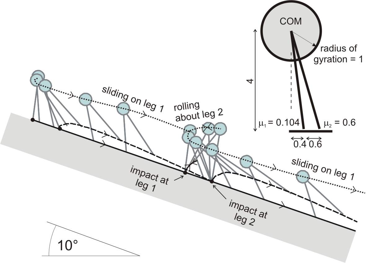
Figure 16: (Adapted from [86]). Simulation of the response of a heavy planar rigid body to a small perturbation of its equilibrium configuration on a perfectly inelastic ($r_{e}=0$) slope. See text for details.

Figure 16 presents simulation results for a specific example of heavy planar rigid body with two contact points that satisfies the strong stability property of [64], yet is not stable in the sense of Lyapunov. The shape of the body is represented by a circle and two lines as in Fig. 15, and for this simulation $r_{e}=0$. Initially, the object is resting on a slope of angle $10^{\circ}$, under the influence of gravity. In this case, a static equilibrium equilibrium in $TT$ mode can be shown to be consistent (calculation omitted). Nevertheless an infinitesimally small state-perturbation may set the object into divergent motion, causing it to tumble down the slope as illustrated. First we find accelerating slip motion on leg 1, in mode $S_{+}F$. This is followed by a sticking impact at leg 2 followed by a rolling motion of that leg (i.e. mode $FT$). This mode continues until leg 1 hits the ground again. These four steps of motion are repeated again and again, while the velocity of the object increases exponentially. The trajectories of the two contact points and the COM are shown by solid, dashed, and dotted curves, respectively in the figure. For more details, see [86]. It is interesting to note that if we had taken a lower coefficient of friction at leg 1, specifically if $\mu_{1}<0.1$, then the initial equilibrium would become ambiguous. Thus at time $t=0$ there would be an additional possibility for the motion, namely the behaviour displayed in the right-hand panels of Fig. 7.

If nothing else, this example illustrates that these considerations of stability with multiple points of contact are not merely of academic interest, but can be easily manifest in purely passive mechanical systems. Another recent practical illustration can be found in the work of Gamos and Or [21]. There they compute many details of the dynamics of bi-pedal passive walkers that can undergo stick-slip transitions, including several cases of multi-stability with complex basins of attraction.

7 Single-point-of-contact case in 3D

Everything discussed so has been for systems whose contact forces and motions line in a plane. Much less is known about the Painlevé paradox in situations that require a fully three-dimensional analysis. For simplicity, we restrict attention to the single contact case. Our goal is to highlight similarities with and differences from the planar case. In what follows we make some general observations, but only do precise calculations in the case of the three-dimensional analogue of the CPP.

7.1 Conditions for Painlevé paradoxes to occur

For any spatial system with a single contact, equations of motion analogous to (8) and (9) can be derived:

$$\dot{u} =a(q,\dot{q},t)+A(q,t)\lambda_{T}+\lambda_{N}B(q,t),$$ (35)

$$\dot{v} =b(q,\dot{q},t)+B^{T}(q,t)\lambda_{T}+\lambda_{N}C(q,t),$$ (36)

where now the tangential velocity $u\in{\mathbb{R}}^{2}$ is a 2-vector, as are $a$, $B$, and $\lambda_{T}$, whereas $A$ becomes a $2\times 2$ matrix. In contrast, quantities involved with normal directions — $v$, $a$, $C$ and $\lambda_{N}$ — remain scalars.

A three-dimensional analogue of the Coulomb friction law can be written in the form

$$\lambda_{T}=-\mu\lambda_{N}\left[\cos\phi\quad\sin\phi\right]^{T},$$ (37)

where $\phi$ is the angle of $u$ relative to the positive $x_{1}$ axis, as in Fig. 17. Equations (36) and (37) imply

$$\dot{v}=b+(C-\mu B^{T}[\cos\phi\quad\sin\phi]^{T})\lambda_{N}=0,$$ (38)

which leads naturally to the definition of the three-dimensional generalisation of the Painlevé parameter

$$p(\phi):=C-\mu B^{T}[\cos\phi\quad\sin\phi]^{T}.$$ (39)

Note that for motion in a plane with angle $\psi$ to the $(x_{1},y)$ plane, as in Fig. 17, sliding in $S_{+}$ mode would correspond to $\phi=\psi$, and sliding in $S_{-}$ mode to $\phi=\psi+\pi$ if $0<\theta<\pi/2$.

Exactly as in the planar case, the free fall mode is consistent if there is no penetration into the contact surface, that is if $b>0$. Moreover the slip mode $S$ is consistent if $\lambda_{N}>0$, which leads to the same condition $bp<0$. Hence, there is a unique consistent mode (either free fall or slip) if $p>0$. In contrast, either both modes are consistent or none of them is consistent if $p<0$.

As an example, consider the three-dimensional analogue of the CPP, namely a slender, rod with uniform cross-section contacting obliquely with a frictional surface. Zhao et al [92] derived the specific equations of motion for such a rod, which when projected onto tangential and normal directions lead (35) and (35) with

$$a =-l\left[\begin{array}[]{c}\dot{\psi}^{2}\cos\psi\cos^{3}\theta+\dot{\theta}^{2}\cos\psi\cos\theta\\ \dot{\psi}^{2}\sin\psi\cos^{3}\theta+\dot{\theta}^{2}\sin\psi\cos\theta\end{array}\right]$$ (42)

$$b =l\dot{\psi}^{2}\sin\theta+l\dot{\theta}^{2}\sin\theta-g$$ (43)

$$A =m^{-1}\left[\begin{array}[]{cc}1+3\sin^{2}\psi+3\cos^{2}\psi\sin^{2}\theta&-3\sin\psi\cos\psi\cos^{2}\theta\\ -3\sin\psi\cos\psi\cos^{2}\theta&1+3\cos^{2}\psi+3\sin^{2}\psi\sin^{2}\theta\end{array}\right]$$ (46)

$$B =3m^{-1}\sin\theta\cos\theta\left[\begin{array}[]{c}\cos\psi\\ \sin\psi\end{array}\right]$$ (49)

$$C =m^{-1}\left(1+3\cos^{2}\theta\right).$$ (50)

Here, $m$ is the mass and $l$ is the half-length of the rod, $\theta$ is the angle between the rod and the horizontal plane. The vectors $u$ and $\lambda_{T}$ are expressed in a global $(x_{1},x_{2})$ reference frame, see Fig. 17.

Let us consider the possibility of the Painlevé paradox for this problem. With the help of (43),(49), (50), the condition $p<0$ for the Painlevé paradox to occur can be expressed as

$$\mu\cos(\phi-\psi)>\mu_{p}(\theta)=\frac{1+3\cos^{2}\theta}{3\cos\theta\sin\theta},$$ (51)

which is identical to the condition for the planar rod (5) if $\phi=\psi$. Thus the Painlevé paradox for the 3D slender rod cannot occur if $\mu\leq\mu_{P}(\theta)$ or if $\cos(\phi-\psi)\leq 0$. In the case of $\mu\geq\mu_{P}(\theta)$ the paradox occurs in a range of slip directions parametrised by $\phi-\psi\in(\phi_{\rm min},\phi_{\rm max})$, where $\phi_{\rm max}=0$ if $\mu=\mu_{P}(\theta)$ and $\phi_{max}$ grows to $\pi/2$ if $\mu\rightarrow\infty$.

It was also shown in [92] that if the rod is in the Painlevé regime with $b<0$, the non-existence paradox (inconsistency) can be resolved by assuming an IWC. This assumption was also justified by taking a compliant contact model similar in fashion to the one introduced in Sec. 4. To obtain a more detailed picture of the dynamics in the Painlevé regime, Shen [72] considered a elastic finite element model of the CPP, using a 3D rod of a finite thickness with a rounded end. He was able to compare the dynamics during planar motion of the system in its plane of symmetry to the dynamics of an equivalent point contact model with a compliant contact point. He also argued that both models show that the continuation in the Painlevé regime can be understood in terms of an IWC.

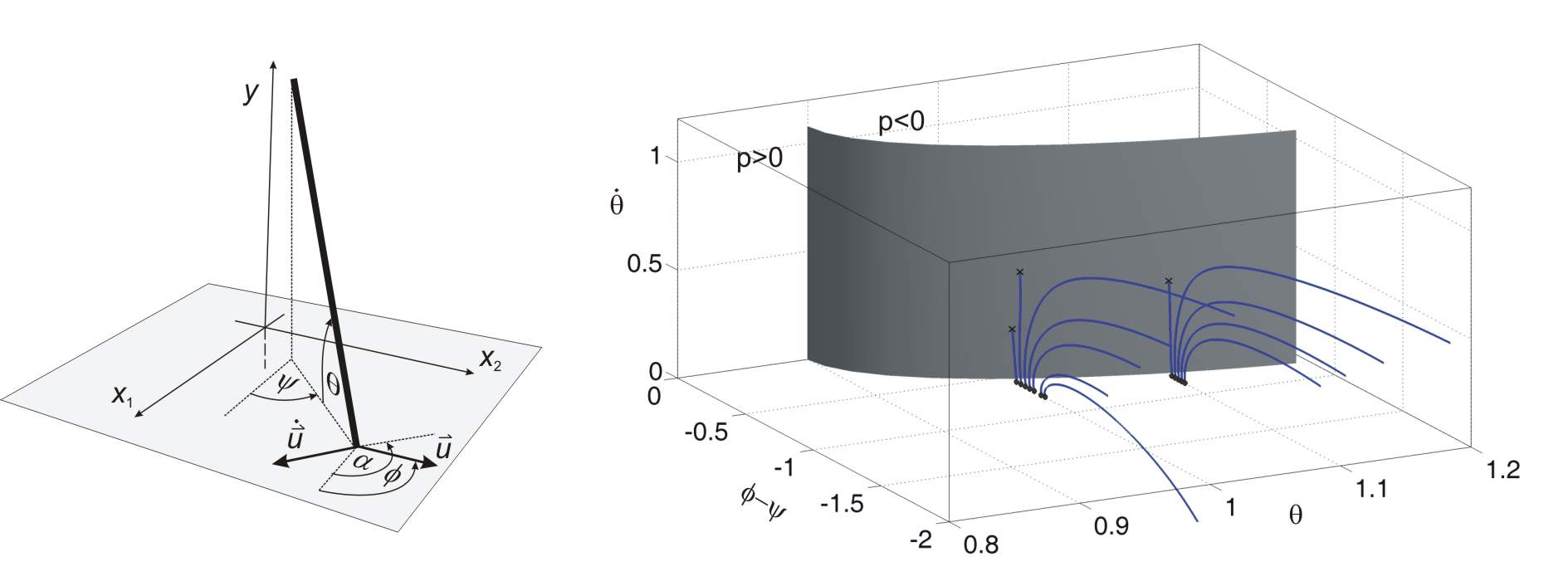
Figure 17: left: a slender, three-dimensional rod slipping on a horizontal surface. The coordinate axes $x_{1}$ and $x_{2}$ are horizontal, whereas axis $y$ is vertical. Here $u$ and $\dot{u}$ are the velocity and the acceleration of the contact point, respectively. Right: simulated trajectories of the slipping rod in a three-dimensional projection of state space, with the boundary of the Painlevé region represented by the grey surface. Circles denote initial points of the trajectories and x-shaped markers indicate points of crossing $p=0$. Parameter values used are $\mu=1$ and radius of gyration $=0.1l$

7.2 Dynamic jam

So far, we have not uncovered any behaviour of 3D systems that is qualitatively different from the planar case, in terms of consistent contact modes or the emergence of IWC. However, when we consider Question 2 from the introduction we get a more subtle answer. In particular, we found in Sec. 5.1, that it was not possible to enter the Painlevé region through the set $p^{+}=0$ while slipping, except at the G-spot where $b$ is simultaneously zero. As we shall now show, this need not be the case for 3D systems.

A fundamental difference that distinguishes the 2D and 3D cases is that for planar systems, the Painlevé parameters $p^{+}$ and $p^{-}$ depend on position variables $q$ and coefficient of friction only. Whereas, note from (39) that $p(\phi)$ in general depends additionally on the generalised velocities $\dot{q}$, through the definition of the angle $\phi$. Note that the angle $\psi$ is a cyclic coordinate of the slipping rod, hence we may assume $\psi=0$ without loss of generality. Then, (35) can be expressed with the help of (42), (46), (49) and (37) as

$$m\dot{u}=-l\cos\theta\left[\begin{array}[]{c}\dot{\psi}^{2}\cos^{2}\theta+\dot{\theta}^{2}\\ 0\end{array}\right]-\mu\lambda_{N}\left[\begin{array}[]{cc}1+3\sin^{2}\theta&0\\ 0&4\end{array}\right]\left[\begin{array}[]{c}\cos\phi\\ \sin\phi\end{array}\right]+3\sin\theta\cos\theta\lambda_{N}\left[\begin{array}[]{c}1\\ 0\end{array}\right]$$ (52)

Assume now that this system is very close to but outside of the Painlevé regime, such that $0<p\ll 1$. Furthermore, the free acceleration is such that the rod remains in contact ($b<0$), which is the case, for example, if the rod has sufficiently small angular velocity. According to (38) we find that $\lambda_{N}=-b/p\gg 1$. Thus, $O(1)$ terms in (52) become negligible in comparison with $O(\lambda_{N})$ terms, yielding

$$-m\lambda_{N}^{-1}\cdot\dot{u} =\mu\left[\begin{array}[]{cc}1+3\sin^{2}\theta&0\\ 0&4\end{array}\right]\left[\begin{array}[]{c}\cos\phi\\ \sin\phi\end{array}\right]-3\sin\theta\cos\theta\left[\begin{array}[]{c}1\\ 0\end{array}\right]+O(\lambda_{N}^{-1})$$ (59)

$$=\mu\left[\begin{array}[]{cc}(1+3\sin^{2}\theta)\mu-3\sin\theta\cos\theta\cos^{-1}\phi&0\\ 0&4\mu\end{array}\right]\left[\begin{array}[]{c}\cos\phi\\ \sin\phi\end{array}\right]+O(\lambda_{N}^{-1}).$$ (64)

The upper left element of the diagonal matrix in is smaller than the lower right one because

$$(1+3\sin^{2}\theta)\mu-3\sin\theta\cos\theta\cos^{-1}\phi\leq(1+3)\mu-0=4\mu.$$ (65)

This means that the absolute value of the angle of the vector that $-\dot{u}$ makes relative to the positive $x_{1}$ axis is larger than the absolute value of the angle $\phi$ of $u$. Therefore, $\phi$ approaches 0 over time in such a way that $\dot{\phi}\cdot\sin\phi<0$. Meanwhile the time derivative of the Painlevé parameter $p$ is (38)

$$\dot{p}=\dot{C}-\frac{d}{dt}\left(\mu B^{T}\right)\left[\cos\phi\quad\sin\phi\right]^{T}-\mu B^{T}\frac{d}{dt}{\left[\cos\phi\quad\sin\phi\right]^{T}}$$

in which all terms are $O(1)$ except for the acceleration-like term $\frac{d}{dt}\left[\cos\phi\quad\sin\phi\right]$, which is $O(\lambda_{N})$. Neglecting the $O(1)$ terms and substituting $\psi=0$ leads to

$$\dot{p} =-\mu B^{T}\frac{d}{dt}{\left[\cos\phi\quad\sin\phi\right]^{T}}+O(1)$$

$$=3\mu m^{-1}\sin\theta\cos\theta\sin\phi\dot{\phi}+O(1),$$

which is negative because $\sin\phi\dot{\phi}<0$ and all other terms are positive. Thus we arrive to the conclusion that $p$ becomes negative, and the system crosses the boundary of the Painlevé regime transversely away from the G-spot. Our conclusion is confirmed by numerical simulation (Fig. 17, right panel). What happens beyond this crossing is an open question.

8 Discussion

This article represents an attempt to survey the state of knowledge on the range complex phenomena in rigid body mechanics that have been grouped together under the epithet of the Painlevé paradox. We have drawn particular attention to recent results by the authors and their collaborators, while trying to establish some general notation and terminology that we hope will help to organise the previous literature and stimulate other researchers to investigate this fascinating topic. Let us close with some philosophical remarks and a brief summary of open problems.

8.1 Philosophical remarks

Far from being resolved, the Painlevé paradox on the inconsistency of rigid body mechanics with frictional contact, first posed over 120 years ago, would seem to retain many open facets. Even for the highly restrictive situation of a planar configuration with a single point contact, we have argued that there remain situations that are undecidable within the framework of rigid body mechanics. In particular, slender bodies such as the classical Painlevé problem of the falling rod reach a point of dynamic jam, from which it is not currently clear whether there is a unique forward continuation without including additional physics. In three dimensions, we have shown that things are even worse, because the rod can enter the unstable Painlevé region transversely. Here, the results in Table 3 suggest there is indeterminacy because the rod could lift-off or take an impact. Also, even outside the Painlevé region, we argued in Sec. 5 that reverse chatter can be triggered at a transition into stick. If reverse chatter occurs then there is infinite degeneracy between a continuum of different phases. Nevertheless, for the single contact case in 2D we showed that inclusion of an impact law and an analysis using contact regularisation enables resolution of all inconsistent cases, but indeterminacy remains.

If one allows more than one contact point, then we indicated in Sec. 6 that there are many other cases of indeterminacy, and we have not yet been able to resolve all possible cases of inconsistency, even under the simplifying assumption that no contact is in stick. We have also provided evidence, for example through the micro-scale chatter-like behaviour of Fig. 15, that there may be far more complex possibilities for reverse or forward chatter-like behaviours in the case of two or more contacts.

One thing that our analysis does point to though is the insufficiency of Kilmister’s principle applied to rigid bodies with multiple contacts. That has led to a common approach in multibody mechanics to seek sufficient conditions under which there is a unique consistent contact mode, thus avoiding any Painlevé paradoxes. We argue that this approach is misguided, because we already know from the single point of contact case that there are easily reachable configurations that are inevitably undecidable and which cannot be resolved without breaking the assumptions of rigid body mechanics. We also showed a specific case in Sec. 6 where there is a unique consistent contact mode $S_{+}S_{+}$, but this is not normally stable and instead an IWC must occur. Rather than seek sufficient conditions to sweep the paradox under the carpet, as it were, we have been motivated instead by the three separate questions posed in the Introduction. In particular we have attempted to separate the questions of: which configurations are consistent or determinate; how one may undergo a transition into an indeterminate state; and whether questions of consistency or indeterminacy can be resolved by consideration of impact and contact regularisation.

Contact regularisation concerns the introduction of finite stiffnesses and in Sec. 4 we considered only the simplest kind, namely introduction of a stiffness in the normal degree of freedom. In one sense such normal regularisation can resolve all of the consequences of the Painlevé paradoxes, if one allows the stiffness to remain finite. Even in this case though, simple nonsmooth friction laws in the tangent direction lead to Filippov systems which can themselves exhibit indeterminacy; see [34] for a mechanical example. The test we have used for genuine determinacy associated with the Painlevé paradox is what we have termed uniform resolvability, namely that normal contact regularisation leads to unique limiting behaviour in the infinite stiffness limit. If such a unique limit does not occur, such as in reverse chatter, then these cases we deem to be genuinely indeterminate. Of course, there are many other possible approaches to regularisation, and we mentioned already the approach of Szalai [82, 81] that appears promising.

We should also stress the fundamental point made in the Introduction that the Painlevé paradox is not about the real world, but an indication of the failure of rigid-body mechanics. Typically any friction or impact law is a gross approximation to tribological processes that occur at the microscale. Thus, the existence of undecidability (either inconsistency or indeterminacy) within a rigid body framework points to situations for which there will be extreme sensitivity with respect to initial conditions in the real mechanics.

An overarching conclusion then is that, for certain configurations at least, a purely rational mechanics approach to rigid body dynamics with impact and friction is fundamentally ill-posed. To put it somewhat pejoratively, one might say that there is nothing “rational” about rational mechanics at least for rigid bodies. There is a strong tradition going back to Newton, Euler and many others in trying to discover the “laws of mechanics” and showing that they are consistent. This body of literature has become known as rational mechanics; and indeed the Archives for Rational Mechanics and Analysis is one of the most prestigious scientific journals. The hope is that one day, by posing sufficiently many constitutive laws one can come up with self-consistent continuum theories for fluids, elastic solids, elasto-plastic materials, etc. One of the simplest such continuum theories is that of rigid body mechanics, which we typically teach to our students through an axiomatic approach. We talk about the Coulomb or Stribeck laws of friction, rather than models of friction. Nevertheless we have shown that with even the simplest consistent friction and impact laws for contact with friction lead to fundamentally undecidable cases, and the search for a grand unifying law that resolves all cases is probably futile.

Rather like Russell & Whitehead’s attempt in Principia Mathematica [89] to systematise arithmetic and, by implication, the whole of mathematics (see, for example [28] for a popular account), we could argue that any mission with the aim rationalising rigid body mechanics through axioms and laws is doomed to failure. Rather like the way Gödel’s Incompleteness Theorem [23] showed the impossibility of Russell and Whithead’s goal, in our view, the inconsistency and indeterminacy that is inherent in the Painlevé paradox suggests that a complete, self-consistent, theory of rigid body mechanics is impossible. It is also tempting to draw the analogy between Gödel’s use of paradox at the heart of his proof. If Gödel’s work has taught us anything it is that no mathematical theory of sufficient complexity to describe the real work is ever complete; undecidability paradoxes are inevitable.

8.2 Open problems and perspectives

In Sec. 2.3 we reviewed some of the configurations that have been shown to exhibit Painlevé paradox phenomena. Many of the practical implications of the theory to these and related mechanisms remain unexplored. For example, is it possible to explain the transition to sprag-slip oscillation in brake-disc-like systems through a reverse chatter instability? Can such instabilities be used to explain the mechanism for drawing dashed lines on a blackboard? Another practical area which seems largely unexplored is in rotor machinery with contact, where there are large couplings between tangential and normal motion due to gyroscopic forces. Even ignoring possible sprag-slip behaviour, rotordyanmics with contact can lead to rich dynamics, see e.g. [95] and references therein.

With two or more contacts we have pointed in Sec. 6 to many new phenomena, including IWCs that can involve one or more contacts and possible micro-chatter. To use a deliberate pun, we have only just scratched the surface for planar bodies with two contacts and there are many cases that remain unexplored. In three dimensions, and for more than two contact points, the conditions that lead to reverse chatter remain completely unexplored. Elucidating when reverse chatter can occur is an important question for applications, for example in the design of grippers and manipulators in robotics. We we have shown, the question of which mode of motion is observed cannot be solved simply by looking at which modes are feasible. Instead, we need to consider Lyapunov stability, which, using the method of contact regularisation, can lead to an understanding of where IWC and/or reverse chatter is either possible or inevitable.

We also pointed to recent work [21] that analyse how Painlevé paradoxes can occur in simple models of legged locomotion. There is a growing body of work in biomechanics that uses ideas from dynamical systems and bifurcation theory to understand human gate stability, since the pioneering work of Alexander [2], see e.g. [49] and references therein for recent results. As yet though, the complexities associated with the Painlevé paradox seems largely unexplored in that literature.

Another practical question is if the extreme sensitivity associated with the Painlevé paradox is unavoidable, how can we design control laws to ameliorate its effects? The state of the art in control of such systems seems to be to use the framework of complementarity or hybrid systems, see for example the work of Heemels and co-workers [26]. However, as we have shown, a complete understanding of the dynamics requires consideration of contact regularisation and impact, which go beyond the complementarity view.

There are many theoretical questions that remain yet to be analysed to determine consistency and stability. As far as we are aware the simplest cases yet to be analysed are situations where there are two sticking contacts in 2D, or where there is just one sticking contact in 3D. In general we are long way from a complete list of types of dynamical behaviour, and it is not yet known whether and how the non-existence paradox can be resolved in all cases. Also, characterisation of bifurcations and transitions in multi-contact systems remains completely unexplored. Implications of Painlevé paradoxes for the much more tricky situations of line or regional contact seem to remain a long way off. Even seemingly simple questions for planar single contact systems remain unsolved, such as what happens beyond the $G$-spot, and whether it is ever possible to cross into $p<0$ other than at this point for systems that have more than three-degrees of freedom.

In summary, far from being resolved, there seems to be a rich array of open questions, both theoretical and practical, that arise from the indeterminacy, multistability and instability associated with the classical Painlevé paradox. If nothing else we hope this survey will serve to stimulate fresh efforts by the next generation of researchers. It would seem to us that there could easily be room for another 120 years of fruitful research on these fascinating phenomena.

References

- [1] V. Acary. Projected event-capturing time-stepping schemes for nonsmooth mechanical systems with unilateral contact and Coulomb’s friction. Computer Methods in Applied Mechanics and Engineering, 256:224–250, 2013.
- [2] R.M. Alexander. A model of bipedal locomotion on compliant legs. Phil. Trans. Roy. Soc. Lond B, 338:189–198, 1992.
- [3] L.S. An. The painlevé paradoxes and the law of motion of mechanical systems with coulomb friction. Journal of Applied Mathematics and Mechanics, 54:430–438, 1990. Translated from Russian original.
- [4] L.X. Anh. Dynamics of Mechanical Systems with Coulomb Friction (Foundations of Engineering Mechanics). Springer, New York, 2003.
- [5] J. Bastien and M. Schatzman. Indeterminacy of a dry friction problem with viscous damping involving stiction. ZAMM, 88:243–255, 2008.
- [6] J.A. Batlle. On Newton’s and Poisson’s rules of percussive dynamics. ASME Journal of Applied Mechanics, 60:376–381, 1993.
- [7] Y. Berdeni. Problems in friction and impact, 2016. Phd Thesis, University of Bristol, in preparation.
- [8] A.V. Borisov and N.A. Kudryashov. Paul Painlevé and his contribution to science. Regular and Chaotic Dynamics, 19:1–19, 2014.
- [9] R.M. Brach. Mechanical Impact Dynamics: Rigid Body Collisions. Wiley, Chichester, UK, 1991.
- [10] B. Brogliato. Nonsmooth Mechanics. Springer, London, 2nd edition, 1999.
- [11] S.J. Burns and P.T. Piiroinen. The complexity of a basic impact mapping for rigid bodies with impacts and friction. Regular and Chaotic Dynamics, 19, 2014.
- [12] T. Butlin and J. Woodhouse. Friction-induced vibration: Model development and comparison with large-scale experimental tests. Journal of Sound and Vibration, 332:5302–5321, 2013.
- [13] A. Chatterjee and A. Ruina. A new algebraic rigid-body collision law based on impulse space considerations. ASME Journal of Applied Mechanics, 65:939–951, 1998.
- [14] R. Cross. ”impact behavior of a superball. American Journal of Physics, 83:238–248, 2015.
- [15] M. di Bernardo, C.J. Budd, A.R. Champneys, and Kowalczyk. Piecewise-smooth dynamical systems; theory and applications. Springer, New York, 2008.
- [16] M. di Bernardo, C.J. Budd, A.R. Champneys, P. Kowalczyk, A.B. Nordmark, G. Olivar, and P.T. Piiroinen. Bifurcations in nonsmooth dynamical systems. SIAM Review, 50:629–701, 2008.
- [17] S. Djerassi. Collision with friction: Part B: Poisson’s and Stornge’s(sic) hypotheses. Multibody Systems Dynamics, 21:37–54, 2009.
- [18] H.A Elkaranshawy. Using self-motion in redundant manipulators to cope with Painlevé paradox. In Biomechanics 2011, 2011. DOI: 10.2316/P.2011.752-076.
- [19] B. Feeny, A. Guran, N. Hinrichs, and K. Popp. A historical review on dry friction and stick-slip phenomena. ASME Applied Mechanics Reviews, 51:321–341, 1998.
- [20] A.F. Filippov. Differential equations with Discontinuous Righthand Sides. Springer, New York, 1988.
- [21] B. Gamos and Y. Or. Dynamic bipedal walking under stick-slip transitions. SIAM Journal of Applied Dynamical Systems, 14:609–642, 2015.
- [22] F. Génot and B. Brogliato. New results on Painlevé paradoxes. European Journal of Mechanics A/Solids, 18:653–677, 1999.
- [23] K. Gödel. Collected works, Vol. I. Oxford University Press, Oxford, UK, 1986. (Containing original German and English translation of: Über formal unentscheidbare Sätze der Principia Mathematica und verwandter Systeme, I. Monatshefte für Mathematik und Physik 38:173–98.).
- [24] S.S. Grigoryan. The solution to the Painlevé paradox for dry friction. Doklady Physics, 46:499–503, 2001. Translated from Russian.
- [25] B. Hall. Why Does Chalk Squeek? Master’s thesis, Department of Engineering Mathematics, University of Bristol, Bristol, UK, 2009.
- [26] W.P.M.H. Heemels, B. De Schutter, J. Lunze, and Lazer. M. Stability analysis and controller synthesis for hybrid dynamical systems. Phil. Trans. Roy. Soc. Lond. A, 368:4937–4960, 2010.
- [27] N. Hoffmann and L. Gaul. A sufficient criterion for the onset of sprag-slip oscillations. Archive of Applied Mechanics, 73:650–660, 2004.
- [28] D.R. Hofstadter. Gödel, Escher, Bach: An Eternal Golden Braid. Penguin, London, 20th edition, 2000.
- [29] W.S. Howard and V. Kumar. On the stability of grasped objects. IEEE Transactions on Robotics and Automation, 12:904–917, 1996.
- [30] R.A. Ibrahim. Friction-induced vibration, chatter, squeal and chaos. Part II: Dynamics and modeling. ASME Applied Mechanics Reviews, 47:227–253, 1994.
- [31] A.P. Ivanov. Energetics of a collision with friction. Journal of Applied Mathematics and Mechanics, 56:527–534, 1992.
- [32] A.P. Ivanov. Singularities in the dynamics of systems with non-ideal constraints. Journal of Applied Mathematics and Mechanics, 67:185–192, 2003.
- [33] Martyn J. and E. Chambers, editors. The Philosophical History and Memoirs of the Royal Academy of Sciences at Paris. J. & P. Knapton, London, 1742.
- [34] M.R. Jeffrey and R. Szalai. Nondeterministic dynamics of a mechanical system. Phys. Rev. E, 90:art. no. 022914, 2014.
- [35] J.H. Jellet. Treatise on the Theory of Friction. Hodges, Foster and Co., Dublin, 1872.
- [36] T.R. Kane. A dynamics puzzle, 1984. Sanford Mechanics Alumni Club Newsletter.
- [37] J.B. Keller. Impact with friction. ASME Journal of Applied Mechanics, 53:1–4, 1986.
- [38] N.M. Kinkaid, O.M. O’Reilly, and Papadopoulos P. Automotic disc brake squeal. Journal of Sound and Vibration, 267:105–166, 2003.
- [39] V.V. Kozlov. Friction by Painlevé and lagrangian mechanics. Doklady Physics, 56:355–358, 2011. Translated from Russian original.
- [40] A. Lamperski and A.D. Ames. Lyapunov theory for zeno stability. IEEE Transactions on Automatic Control, 58:101–115, 2013.
- [41] J. Le Rouzic, A. Le Bot, J. Perret-Liaudet, M. Guibert, A. Rusanov, L. Douminge, F. Bretagnol, and D. Mazuyer. Friction-induced vibration by Stribeck’s law: Application to wiper blade squeal noise. Tribology Letters, 49:563–572, 2013.
- [42] R. Leine and H. Nijmeijer. Dynamics and Bifurcations of Non-Smooth Mechanical Systems. Springer, New York, 2004.
- [43] R.I. Leine, B. Brogliato, and H. Nijmeijer. Periodic motion and bifurcations induced by the Painlevé paradox. European Journal of Mechanics A/Solids, 21:869–896, 2002.
- [44] RI Leine and N van de Wouw. Stability properties of equilibrium sets of non-linear mechanical systems with dry friction and impact. Nonlinear Dynamics, 51(4):551–583, 2008.
- [45] J. Liang, O. Ma, and C. Liu. Relative contact dynamics and its application on manipulator’s contact stability problem. In ASME 2012 International Design Engineering Technical Conferences, Chicago, USA, 2012.
- [46] C.S. Liu, Z. Zhao, and B. Chen. The bouncing motion appearing in a robotic system with unilateral constraint. Nonlinear Dyanamics, 49:217–232, 2007.
- [47] P. Lötstedt. Mechanical systems of rigid bodies subject to unilateral constraints. SIAM J. Applied Math., 42:281–296, 1982.
- [48] I.S. Mamaev and T.B. Ivanova. The dynamics of a rigid body with a sharp edge in contact with an inclined surface in the presence of dry friction. Regular and Chaotic Dynamics, 19:116–139, 2014.
- [49] H.M. Maus, S. Revzen, J. Guckenheimer, C. Ludwig, Reger J., and Seyfarth A. Constructing predictive models of human running. Royal Society Interface, 12:Art. No. UNSP 20140899, 2015.
- [50] J. Melcher, A.R. Champneys, and D.J. Wagg. The impacting cantilever: modal non-convergence and the importance of stiffness matching. Phil. Trans. Roy. Soc. Lond. A, 371:Art. No. 20120434, 2013.
- [51] P.D. Moreau, J.J. Panagiotopoulos. Nonsmooth Mechanics and Applications. Springer, New York, 1988. CISM Courses and Lectures vol. 302.
- [52] Yu.I. Neimark and V.N. Smirnova. Singularly perturbed problems and the Painlevé paradox. Differential Equations, 36:1639–1646, 2000.
- [53] A. Nordmark, H. Dankowicz, and Champneys A. Discontinuity-induced bifurcations in systems with impacts and friction: Discontinuities in the impact law. Int. J. Nonlinear Mech., 44:1011–1023, 2009.
- [54] A. Nordmark, H. Dankowicz, and A. Champneys. Discontinuity-induced bifurcations in systems with impacts and friction; part iii, 2011. Unpublished notes.
- [55] A. Nordmark, H. Dankowicz, and A. Champneys. Friction-induced reverse chatter in rigid-body mechanisms with impacts. IMA Journal of Applied Mathematics, 76:85–119, 2011.
- [56] A.B. Nordmark and P.T. Piiroinen. Simulation and stability analysis of impacting systems with complete chattering. Nonlinear Dynamics, 58:85–106, 2009.
- [57] Y. Or. Painlevé’s paradox and dynamic jamming in simple models of passive dynamic walking. Regular and Chaotic Dynamics, 19:64–80, 2014.
- [58] Y. Or and E. Rimon. On the hybrid dynamics of planar mechanisms supported by frictional contacts I: Necessary conditions for stability. In Proc. IEEE International Conference on Robotics and Automation, pages 1213 – 1218, 2008.
- [59] Y. Or and E. Rimon. On the hybrid dynamics of planar mechanisms supported by frictional contacts II: Stability of two-contact rigid body postures. In Proc. IEEE International Conference on Robotics and Automation, pages 1219–1224, 2008.
- [60] Y. Or and E. Rimon. Investigation of Painlevé’s paradox and dynamic jamming during mechanism sliding motion. Nonlinear Dyn., 67:1647–1668, 2012.
- [61] P. Painlevé. Sur les loi du frottement de glissement. Comptes Rendu des Séances de l’Academie des Sciences, 121:112–115, 1895.
- [62] P. Painlevé. Sur les loi du frottement de glissement. Comptes Rendu des Séances de l’Academie des Sciences, 141:401–405, 1905.
- [63] P. Painlevé. Sur les loi du frottement de glissement. Comptes Rendu des Séances de l’Academie des Sciences, 141:546–552, 1905.
- [64] J.S. Pang and J. Trinkle. Stability characterizations of rigid body contact problems with coulomb friction. Zeitschrift Angewandte Mathematik Mechanik, 80:643–663, 2000.
- [65] F. Pfeiffer and C. Glocker. Multibody Dynamics with Unilateral Contacts. Wiley, Chichester, ?? edition, 2008.
- [66] S.D. Poisson. Traité de Mécanique. Courier, Paris, 1811.
- [67] T.J. Prescott, M.J. Pearson, B. Mitchinson, and A.G. Sullivan, JCW ad Pipe. Whisking with robots. IEEE Robotics & Automation Magazine, 16:42–50, 2009.
- [68] T. Putelat and J.H.P. Dawes. Steady and transient sliding under rate-and-state friction. J. Mech. Phys. Solids, 78:70–93, 2015.
- [69] J. Sanders. A study of chatter-induced loss of mechanical contact, 2013. MS thesis, Theoretical & Applied Mechanics, University of Illinois at Urbana-Champaign.
- [70] T. Schindler and V. Acary. Timestepping schemes for nonsmooth dynamics based on discontinuous galerkin methods: Definition and outlook. Mathematics and Computers in Simulation, 95:180–199, 2014.
- [71] T. Schnidler, B. Nguyen, and J. Trinkle. Understanding the difference between prox and complementarity formulations for simulation of systems with contact. In IEEE/RSJ International Conference on Intelligent Robotics and Systems, San Francisco, USA, 2011.
- [72] Y. Shen. Painlevé paradox and dynamic jam of a three-dimensional elastic rod. Archive of Applied Mechanics, 85:805–816, 2015.
- [73] Y.N.A. Shen and W.J. Stronge. Painleve paradox during oblique impact with friction. Eur. J. Mechanics A – Solids, 30:457–467, 2011.
- [74] D.E. Stewart. Existence of solutions to rigid body dynamics and the Painlevé paradoxes. Comptes Rendus de l’Acedemie des Science Serie I: Matheamtique, 325:689–693, 1997.
- [75] D.E. Stewart. Convergence of a time-stepping scheme for rigid-body dynamics and resolution of Painlevé’s problem. Archive for Rational Mechanics and Analysis, 145:215–260, 1998.
- [76] D.E. Stewart. Rigid-body dynamics with friction and impact. SIAM Review, 42:3–39, 2000.
- [77] W.J. Strong. Smooth dynamics of oblique impact with friction. International Journal of Impact Engineering, 51:36–49, 2013.
- [78] W.J. Stronge. Rigid body collisions with friction. Proceedings of the Royal Society of London, 431:169–181, 1990.
- [79] W.J. Stronge. Impact Mechanics. Cambridge University Press, Cambridge, UK, 2000.
- [80] W.J. Stronge. Energetically consistent calculations for oblique impact in unbalanced systems with friction. J. Applied Mechanics – Trans. ASME, 82:art. no. 081003, 2015.
- [81] R. Szalai. Impact mechanics of elastic structures with point contact. Journal of Vibration and Acoustics — Transactions of the ASME, 136:Art. No. 041002, 2014.
- [82] R. Szalai. Modelling elastic structures with strong nonlinearities with application to stick-slip friction. Proc. Roy Soc. Lond. A, 470:Art. No. 20130593, 2014.
- [83] P.L. Várkonyi. Dynamics of rigid bodies with multiple frictional contacts: extended analysis, 2015. unpublished notes.
- [84] P.L. Várkonyi. Dynamics of rigid bodies with multiple frictional contacts: new faces of painlevé’s paradox. In Proc. 13th International Conf. of Dynamical Systems: theory and applications (DSTA), 2015.
- [85] P.L. Várkonyi. On the stability of rigid multibody systems with applications to robotic grasping and locomotion. ASME Journal of Mechanisms and Robotics, 7:041012, 2015.
- [86] P.L. Várkonyi, D. Gontier, and J. W. Burdick. On the lyapunov stability of quasistatic planar biped robots. In IEEE International Conference on Robotics and Automation (ICRA), pages 63–70, 2012.
- [87] P.L. Várkonyi and Y. Or. Lyapunov stability of a rigid body with two frictional contacts, 2015. unpublished notes.
- [88] A. Wagner, E. Heffel, A.F. Arrieta, G. Spelsberg-Korspeter, and P. Hagedorn. Analysis of an oscillatory Painlevé-Klein apparatus with a nonholonomic constraint. Differential Equations and Dynamical Systems, 21:149–157, 2013.
- [89] A.N. Whitehead and B. Russell. Principia Mathematica. Cambridge University Press, Cambridge, UK, second edition, 1927.
- [90] E.V. Wilms and H. Cohen. The occurrence of Painlevé’s paradox in the motion of a rotating shaft. J. Appl. Mech., 64:1008–1010, 1997.
- [91] J. Woodhouse, T. Putelat, and A. McKay. Are there reliable constitutive laws for dynamic friction?, 2015. to appear in Phil. Trans. Roy. Soc. Lond A.
- [92] Z. Zhao, C. Liu, and B. Chen. The Painlevé paradox studied at a 3d slender rod. J. Applied Mechanics – Trans. ASME, 75:art. no. 041006, 2008.
- [93] Z. Zhao, C. Liu, B. Chen, and B. Brogliato. Asymptotic analysis of Painlevé’s paradox. Multibody System Dynamics, Published online:DOI: 10.1007/s11044–014–9448–1, 2015.
- [94] Z. Zhao, C.S. Liu, W. Ma, and B. Chen. Experimental investigation of the Painlevé paradox in a robotic system. J. Applied Mechanics – Trans. ASME, 75:art. no. 041006, 2008.
- [95] A. Zilli, R.J. Williams, and David J. Ewins. Nonlinear dynamics of a simplified model of an overhung rotor subjected to intermittent annular rubs. J. Eng. Gas Turbines Power – Transactions ASME, 137:Art. No. 065001, 2015.