Thermodynamic formalism and linear response theory
for non-equilibrium steady states

Abstract

We study the linear response in systems driven away from thermal equilibrium into a non-equilibrium steady state with non-vanishing entropy production rate. A simple derivation of a general response formula is presented under the condition that the generating function describes a transformation that (to lowest order) preserves normalization and thus describes a physical stochastic process. For Markov processes we explicitly construct the conjugate quantities and discuss their relation with known response formulas. Emphasis is put on the formal analogy with thermodynamic potentials and some consequences are discussed.

I Introduction

One of the objectives of computational sciences is the accurate prediction of material properties. The determination of transport coefficients (e.g., conductivities and mobilities) remains a challenge since, in general, it implies currents and thus non-equilibrium conditions. Illustrative as well as technologically important examples include the efficient transport of charges in organic semiconductors Coropceanu et al. (2007); Poelking et al. (2014) and across thin membranes in reverse osmosis Kalra et al. (2003). While many sophisticated numerical methods have been developed based on thermal equilibrium, for driven systems one typically has to resort to brute-force computer experiments.

Sufficiently close to equilibrium transport coefficients can be determined from equilibrium fluctuations via the fluctuation-dissipation theorem Kubo et al. (1991). There have been considerable efforts to find general principles also for the linear response of non-equilibrium states Speck and Seifert (2006); Baiesi et al. (2009); Chetrite and Gawedzki (2009); Prost et al. (2009); Speck (2010); Seifert (2011); Warren and Allen (2012) (for more complete reviews we refer to Refs. 12; 13; 14 and references therein), which find application in “field-free” numerical algorithms Chatelain (2003); Diezemann (2005); Berthier (2007). There is now a “zoo” of different approaches and derivations yielding (sometimes unrecognized) equivalent results. One reason might be that actually several conjugate observables (and their linear combinations) are equivalent in determining the response Seifert and Speck (2010).

Extending the notion of statistical ensembles to trajectories (time-ordered sequences of dynamic events) is currently receiving considerable attention Lecomte et al. (2007); Garrahan et al. (2009); Turner et al. (2014). A canonical structure for the joint probability of microscopic probabilities and their currents as been formulated in Ref. 22. In contrast, here we are concerned with macroscopic currents without information about microscopic probabilities (or densities). Another concept is that of “canonical” path ensembles (also appearing under the names $s$-ensemble Merolle et al. (2005); Garrahan and Lesanovsky (2010), tilted ensemble, or Esscher transform) in which trajectories are biased by a time-integrated observable. Under certain conditions typical trajectories in the canonical path ensemble are equivalent to trajectories in the original processes with fixed value of the observable Chetrite and Touchette (2013, 2014); Szavits-Nossan and Evans (2015); Garrahan (2016). The purpose of this paper is to follow these ideas and apply them to the linear response around a non-equilibrium steady state (NESS). It is organized as follows: First, we briefly outline the canonical structure of intensive affinities and extensive generalized distances for NESS. We then derive a general response formula and show that it contains previously derived results, in particular the response formula by Warren and Allen Warren and Allen (2012) and the path weight representation Baiesi et al. (2009); Seifert and Speck (2010); Baiesi and Maes (2013). Before concluding we discuss our results in the light of a possible thermodynamic formalism for NESS.

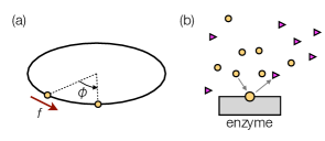
Figure 1: Examples for affinities and distances. (a) Colloidal particle in a ring trap with radius $R$. The particle is driven by a constant force $f$ (the affinity) while $X_{\tau}=R\phi$ is the total distance travelled during time $\tau$. (b) Sketch of an enzyme driving the reaction $\circ\to\triangleright$. The generalized “distance” $X_{\tau}=N^{\triangleright}_{\tau}=-N^{\circ}_{\tau}$ now corresponds to the number of $\triangleright$ molecules produced during time $\tau$. The affinity $f=-(\mu^{\triangleright}-\mu^{\circ})$ is given by the difference of chemical potential, which we assume to be fixed by chemiostats.

II Thermodynamic formalism

II.1 Conjugate variables

The mathematical structure of equilibrium statistical mechanics is based on pairs of an extensive quantity (volume, particle number) and the conjugate intensive quantity (pressure, chemical potential), which are related through thermodynamic potentials (free energies). What makes the formalism so powerful is that these potentials are also generating functions encoding the full statistics of the non-conserved extensive quantities. As a corollary, fluctuations encode the response of thermodynamic observables to a small external perturbation.

Pairs of apparently conjugate quantities $(f^{i},X^{i})$ also arise for non-equilibrium steady states (NESS), where non-zero intensive affinities $f^{i}$ (the generalized forces) give rise to transport and thus extensive (generalized) distances $X^{i}_{\tau}\sim\tau$ (measured over time $\tau$), see Fig. 1 for two examples. Their product determines the entropy production $\Sigma_{\tau}=\sum_{i}f^{i}X^{i}_{\tau}$. Truly conjugate quantities, however, would require the existence of a non-equilibrium “potential” $\Phi(f;\tau)$ so that $\langle X^{i}_{\tau}\rangle=\frac{\partial\Phi}{\partial f^{i}}$, which more generally would determine state functions and justify variation principles Martyushev and Seleznev (2006); Sasa and Tasaki (2006). Since this also implies strict convexity, it would preclude established phenomena like a negative differential mobility Jack et al. (2008).

II.2 Linear response regime

A thermodynamic description does, however, apply to the linear response regime. To this end, consider a generalized distance $X_{\tau}\sim\tau$ measured in thermal equilibrium (i.e., $f=0$) with probability distribution $P_{0}(X;\tau)$. Clearly, the average $\langle X_{\tau}\rangle=0$ vanishes. The time $\tau$ now plays a role similar to system size $N$ in conventional statistical mechanics. We define the generating function

$$Z_{0}(f;\tau)\equiv\int\mathrm{d}X\;e^{\frac{1}{2}fX}P_{0}(X;\tau)\asymp e^{\tau\frac{1}{2}\sigma(f)}$$ (1)

with large deviation function $\sigma(f)$, where $\asymp$ denotes the asymptotic limit of $\tau$ becoming larger than the longest correlation time. Following the analogy with conventional thermodynamics we ask: Does $Z_{0}(f;\tau)$ for $f\neq 0$ describe the same physical system but now with non-zero affinity (i.e., driven into a NESS)? A positive answer would imply that

$$\langle X_{\tau}\rangle=\tau\frac{\partial\sigma}{\partial f}$$ (2)

holds, which, however, is not the case for arbitrary $f$. Only for small $|f|\ll 1$ in the linear response regime does such an interpretation yield the correct result with mean

$$\begin{split}\langle X_{\tau}\rangle&=\frac{1}{Z_{0}}\int\mathrm{d}X\;Xe^{\frac{1}{2}fX}P_{0}(X;\tau)\\ &=\frac{1}{2}\langle(X_{\tau})^{2}\rangle f+\mathcal{O}(f^{2}).\end{split}$$ (3)

This result is the well-known fluctuation-dissipation theorem Kubo et al. (1991) through which fluctuations in thermal equilibrium determine how the system reacts to a small applied force $f$. Indeed, Onsager’s seminal insight has been that in the linear response regime (half) “the rate of increase of the entropy plays the role of a potential” Onsager (1931), namely the large deviation function

$$\sigma(f)=\frac{1}{2}\sum_{ij}L^{ij}f^{i}f^{j}$$ (4)

with symmetric Onsager coefficients $L^{ij}=L^{ji}$ following from the Green-Kubo relations

$$\frac{\partial}{\partial\tau}\frac{1}{2}\langle X^{i}_{\tau}X^{j}_{\tau}\rangle\asymp L^{ij}.$$ (5)

II.3 Canonical path ensembles

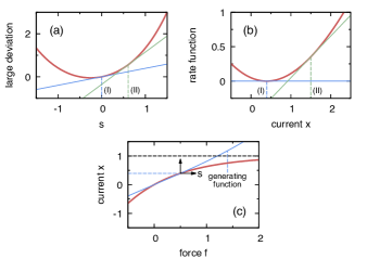
Figure 2: Illustration of the duality of $s$ and current $x=X_{\tau}/\tau$ for the asymmetric random walk (for details see Appendix A, with $f=\tfrac{1}{2}$ and $k^{+}=1$): (a) Large deviation function $\phi_{f}^{\ast}(s)$ (thick line). The slope at $s=0$ (steady state I) corresponds to the mean current $x_{0}$. (b) Rate function $\phi_{f}(x)$ of the current (thick line) with minimum at $x_{0}$. Conditioning currents to a value $x_{s}>x_{0}$ leads to the steady state (II) with $s>0$ determined by the slope. (c) The unbiased average current as a function of driving force $f$ (thick line) and the current $x_{s}=\partial_{s}\phi_{f}^{\ast}$ (thin line) from the generating function, where $s=(f_{\text{eff}}-f)/2$ quantifies a perturbation of the steady state with effective force $f_{\text{eff}}$. Both currents agree for $s=0$ but deviate for increasing values of the perturbation $s$. For fixed $k^{+}$ the unbiased current is bounded (dashed black line).

Away from the linear response regime for NESS characterized by the affinities $f$ we can still define the generating function

$$Z_{f}(s;\tau)\equiv\int\mathrm{d}X\;e^{sX}P_{f}(X;\tau)\asymp e^{\tau\phi_{f}^{\ast}(s)},$$ (6)

where $s$ at this point is just the argument of this function. Moments and cumulants are obtained through differentiation with respect to $s$ around $s=0$. The function $\phi_{f}^{\ast}(s)$ is the large deviation function, which by construction is a convex function. It is related to the rate function $P_{f}(X;\tau)\asymp e^{-\tau\phi_{f}(x)}$ for the current $x\equiv X_{\tau}/\tau$ through the Legendre-Fenchel transform Touchette (2009)

$$\phi_{f}^{\ast}(s)=\sup_{x}[xs-\phi_{f}(x)].$$ (7)

One can now ask the following question: Assume that we condition the path ensemble to contain only trajectories with a fixed value $x_{s}$ for the current. As discussed in detail by Chetrite and Touchette Chetrite and Touchette (2013, 2014), in the limit of large $\tau$ this “microcanonical” ensemble becomes equivalent (under mild assumptions) to a “canonical” ensemble in which the current fluctuates but its mean equals $x_{s}$. This canonical path ensemble is described through the generating function Eq. (6) for a value of $s$ determined through the condition $s=\partial_{x}\phi_{f}|_{x_{s}}$. While $s$ and $x$ are thus conjugate quantities (see Fig. 2 for an illustration for a specific system), changing $s$ does not trace a change of the affinities but involves a rather complicated, non-local transformation (Doob’s transform) also of the interactions Jack and Sollich (2010); Speck and Garrahan (2011); Chetrite and Touchette (2013, 2014); Nyawo and Touchette (2016). It is exactly this behavior that complicates a general thermodynamic description of NESS. However, in the following we demonstrate that small $s$ can be interpreted as a perturbation of the steady state, leading trivially to linear response relations. Moreover, based on this result we can construct a different set of conjugate quantities which extend Onsager’s result to NESS driven beyond the linear response regime.

III A general response formula

We consider a steady state maintained by at least one non-vanishing affinity and thus having a non-vanishing entropy production rate $\langle\Sigma_{\tau}\rangle>0$. For clarity, in this section we consider a single perturbation but the generalization to more than one is straightforward. To be sufficiently general, we define our quantity of interest through the stochastic (Riemann-Stieltjes) integral of the form

$$R_{\tau}[\omega_{t}]\equiv\int_{0}^{\tau}\mathrm{d}r(\omega_{t})\;=\int_{0}^{\tau}\mathrm{d}t\;\dot{r}(\omega_{t},\dot{\omega}_{t})$$ (8)

over a process $\omega_{t}$ representing the state $\omega$ of the system at time $t$. The integral maps a single trajectory $\{\omega_{t}\}_{0}^{\tau}$ of length $\tau\geqslant 0$ onto a real number. Clearly, $R_{\tau}\sim\tau$ is a time-extensive quantity. It will be convenient later to also introduce the generalized velocity $\dot{r}(\omega,\dot{\omega})$, which for stochastic processes is to be understood symbolically and follows the notational convention that typically is used in physics.

The joint probability $\phi(\omega,R,t)$ describes the probability to observe the system in state $\omega$ at time $t$ having accumulated an amount $R=R_{t}$ up to time $t\leqslant\tau$ starting with $R_{0}=0$. Hence, the initial condition factorizes to $\phi(\omega,R,0)=\psi(\omega)\delta(R)$, where $\psi(\omega)$ is the steady state probability of state $\omega$ and $\delta(R)$ is the Dirac $\delta$-function.

It is often more convenient to work with the (Laplace) transform

$$\hat{\phi}_{s}(\omega,t)\equiv\int\mathrm{d}R\;e^{sR}\phi(\omega,R,t)$$ (9)

with initial condition $\hat{\phi}_{s}(\omega,0)=\psi(\omega)$ following from the factorization of the joint probability, where the integral runs over all possible values of $R$. Moreover, for $s=0$ we have that $\hat{\phi}_{0}(\omega,t)=\psi(\omega)$ is the steady state probability. While in general $\hat{\phi}_{s}(\omega,t)$ is not normalized, we now explore the consequences of demanding that $\hat{\phi}_{s}(\omega,t)$ remains a normalized function for $s\neq 0$. Since for non-negative $\phi(\omega,R,t)$ Eq. (9) implies that also $\hat{\phi}_{s}(\omega,t)$ is non-negative, it can be interpreted as the probability distribution of state $\omega$ for a system parametrized by $s$. At this point the physical meaning of $s$ is not obvious but in the next section we will construct explicitly conjugate pairs $(s,R)$.

Now consider a system described by the probability distribution $\hat{\phi}_{s}(\omega,t)$. The expectation value for an arbitrary observable $A(\omega)$ becomes

$$\langle A(t)\rangle_{s}=\sum_{\omega}A(\omega)\hat{\phi}_{s}(\omega,t),$$ (10)

which reduces to $\langle A\rangle$ for $\hat{\phi}_{0}(\omega,t)=\psi(\omega)$ at $s=0$. Hence, in the following we interpret the conjugate variable $s$ appearing in the generating function to describe an external perturbation applied to the system at $t=0$ and driving it towards a neighboring steady state. The response to this perturbation is

$$\begin{split}\left.\frac{\partial\langle A(\tau)\rangle_{s}}{\partial s}\right|_{s=0}&=\sum_{\omega}A(\omega)\left.\frac{\partial\hat{\phi}_{s}(\omega,\tau)}{\partial s}\right|_{s=0}\\ &=\sum_{\omega}\int\mathrm{d}R\;A(\omega)R\phi(\omega,R,\tau)\\ &=\langle A(\tau)R_{\tau}\rangle,\end{split}$$ (11)

which follows inserting Eq. (9). This is our central result. It relates the response (sometimes called sensitivity) of an observable to the correlations of this observable with the amount of $R$ accumulated since the perturbation was applied. The correlations are to be determined in the unperturbed steady state corresponding to $s=0$. The result Eq. (11) is quite general and does not require any assumptions on the dynamics.

IV Constructing conjugate pairs

The response Eq. (11) follows for functions $\hat{\phi}_{s}(\omega,t)$ that, at least for small $s$, are normalized. This places some restrictions onto what integrals $R_{\tau}[\omega_{t}]$ are actually admissible. One property follows immediately by choosing $A(\omega)=1$, which implies that the average $\langle R_{t}\rangle=0$ vanishes for any $t>0$.

IV.1 Stochastic dynamics

To be more specific, we consider a continuous Markov process

$$\mathrm{d}\omega_{t}=\mathcal{F}(\omega_{t})\mathrm{d}t+\mathrm{d}\xi(\omega_{t})$$ (12)

with effective drift vector $\mathcal{F}(\omega)$ and random increments

$$\mathrm{d}\xi(\omega)=\sum_{\alpha}\sigma_{\alpha}(\omega)\circ\mathrm{d}W_{\alpha}(t),$$ (13)

where $W_{\alpha}(t)$ are independent Wiener processes and the symbol $\circ$ denotes the Stratonovich rule for stochastic integrals. With the symmetric diffusion matrix

$$D^{ij}(\omega)\equiv\frac{1}{2}\sum_{\alpha}\sigma_{\alpha}^{i}(\omega)\sigma_{\alpha}^{j}(\omega)$$ (14)

the Markov generator reads

$$L_{0}=F\cdot D\cdot\nabla+\nabla\cdot D\cdot\nabla=(F+\nabla)\cdot D\cdot\nabla.$$ (15)

Its adjoint $L^{\dagger}_{0}$ generates the time evolution of the probability distribution, $\partial_{t}\psi=L^{\dagger}_{0}\psi$. Here, $F(\omega)$ is the physical force such that the effective drift becomes

$$\mathcal{F}=D\cdot F+\frac{1}{2}\sum_{\alpha}(\nabla\cdot\sigma_{\alpha})\sigma_{\alpha}.$$ (16)

Throughout we set Boltzmann’s constant and temperature to unity so that entropies are dimensionless and the mobility matrix coincides with the diffusion matrix Eq. (14).

IV.2 The response formula of Warren and Allen

We first consider

$$\mathrm{d}r(\omega)=h(\omega)\mathrm{d}t+g(\omega)\circ\mathrm{d}\xi(\omega),$$ (17)

where the vector $g(\omega)$ couples to the same noise as in Eq. (12). Following Chetrite and Touchette Chetrite and Touchette (2013, 2014), the tilted (or deformed) generator for the evolution $\partial_{t}\hat{\phi}_{s}=L^{\dagger}_{s}\hat{\phi}_{s}$ becomes

$$L_{s}=F\cdot D\cdot\nabla+(\nabla+sg)\cdot D\cdot(\nabla+sg)+sh,$$ (18)

which for $s=0$ reduces to the generator $L_{0}$ in Eq. (15). Expanding the second term to linear order of $s$, we can recast this generator into the form

$$L_{s}=(F+2sg+\nabla)\cdot D\cdot\nabla+s[\nabla\cdot(D\cdot g)+h]+\mathcal{O}(s^{2}),$$ (19)

which manifestly preserves normalization if $\nabla\cdot(D\cdot g)+h=0$, which thus determines $h(\omega)$. Note that changing from Stratonovich to Itô calculus, this condition implies that $\mathrm{d}r=g\cdot\mathrm{d}\xi$. Clearly, since then state and noise are independent, the expectation value of $R$ vanishes as required.

We now assume that the perturbed steady state is described by the forces $F_{s}(\omega)$ depending on $s$. Expanding the forces to linear order,

$$F_{s}(\omega)=F(\omega)+s\left.\frac{\partial F_{s}(\omega)}{\partial s}\right|_{s=0}+\mathcal{O}(s^{2}),$$ (20)

we read off the coefficient

$$g(\omega)=\frac{1}{2}\left.\frac{\partial F_{s}(\omega)}{\partial s}\right|_{s=0}$$ (21)

by comparing with Eq. (19). This is the result found in Ref. 11 following quite a different approach. Provided we know how the forces depend on $s$, we have thus constructed one possible observable $R_{\tau}$ to be used in Eq. (11).

IV.3 Coupling to state changes

A more general form of time-extensive observables is given by

$$\mathrm{d}r(\omega)=h(\omega)\mathrm{d}t+g(\omega)\circ\mathrm{d}\omega,$$ (22)

where the vector $g(\omega)$ now couples to the evolution of the state $\omega$. The generator follows as

$$L_{s}=F\cdot D\cdot(\nabla+sg)+(\nabla+sg)\cdot D\cdot(\nabla+sg)+sh.$$ (23)

Expanding to lowest order we again find Eq. (21) for the coefficient $g(\omega)$ and the condition to preserve normalization now becomes

$$F\cdot D\cdot g+\nabla\cdot(D\cdot g)+h=0.$$ (24)

It is straightforward to check that the time-integrated observable $R_{\tau}$ following from Eq. (22) can be written as the derivative

$$R_{\tau}=-\left.\frac{\partial\mathcal{A}_{\tau}}{\partial s}\right|_{s=0}$$ (25)

with stochastic action

$$\mathcal{A}_{\tau}[\omega_{t}]\equiv\int_{0}^{\tau}\mathrm{d}t\;\mathcal{L}_{s}(\omega_{t},\dot{\omega}_{t}),$$ (26)

where (still employing the Stratonovich rule)

$$\mathcal{L}_{s}(\omega,\dot{\omega})=\frac{1}{4}(\dot{\omega}-D\cdot F_{s})\cdot D^{-1}\cdot(\dot{\omega}-D\cdot F_{s})\\ +\frac{1}{2}\nabla\cdot(D\cdot F_{s}).$$ (27)

Hence, employing Eq. (22), the conjugate observable $R_{\tau}$ now corresponds to the “path weight representation” discussed in Refs. 6; 18; 14.

V Discussion

V.1 Thermodynamic formalism

It is straightforward to extend Eq. (11) to multiple affinities $s=\{s^{i}\}$. We restrict our considerations to the set of observables $\{R^{i}_{\tau}\}$ with vanishing mean, for which we can derive a local potential. To this end, from the transformed joint probability Eq. (9) we define the generating function

$$Z_{f}(s;\tau)=\sum_{\omega}\hat{\phi}_{s}(\omega,\tau)\asymp e^{\tau\varphi_{f}^{\ast}(s)},$$ (28)

where we make explicit the dependency on the affinities $f$ driving the system. In the limit $\tau\to\infty$ the large deviation function again follows from the Legendre-Fenchel transform

$$\varphi_{f}^{\ast}(s)=\sup_{r}\left[r\cdot s-\varphi_{f}(r)\right],$$ (29)

where we have assumed that a large deviation principle $P_{f}(R;\tau)\asymp e^{-\tau\varphi_{f}(r)}$ holds with $r^{i}\equiv R^{i}/\tau$. As a consequence, $\varphi_{f}^{\ast}(s)$ is always a convex function and constitutes our local potential around a steady state determined by the affinities $f$. For a potential $\varphi_{f}^{\ast}(s)$ that is differentiable at $s=0$, the correlations are manifestly symmetric and follow as

$$\langle R^{i}_{\tau}R^{j}_{\tau}\rangle=\left.\frac{\partial^{2}}{\partial s^{i}\partial s^{j}}\ln Z_{f}\right|_{s=0}\asymp\left.\tau\frac{\partial^{2}\varphi_{f}^{\ast}}{\partial s^{i}\partial s^{j}}\right|_{s=0}=\tau L_{f}^{ij}$$ (30)

with steady state susceptibilities

$$L_{f}^{ij}\equiv\lim_{\tau\rightarrow\infty}\frac{1}{\tau}\frac{\partial\langle R^{i}_{\tau}\rangle_{s}}{\partial s^{j}}=\frac{\partial\langle\dot{r}^{i}\rangle_{s}}{\partial s^{j}}.$$ (31)

This result extends the Onsager potential Eq. (4) to non-zero affinities and emphasizes the canonical structure. An interesting consequence is that, employing Legendre transforms as in conventional thermodynamics, we can now switch between affinity $s^{i}$ and current $\langle\dot{r}^{i}\rangle$ depending on what is the more convenient variable for a specific situation. Moreover, susceptibilities are related by Maxwell and further relations (similar to, e.g., the relation between the heat capacities at constant volume and constant pressure).

V.2 Illustration: Single particle in a ring trap

To briefly illustrate our results we consider the paradigmatic single colloidal particle moving in a ring trap Blickle et al. (2007); Gomez-Solano et al. (2009, 2011); Nyawo and Touchette (2016), see Fig. 1(a). The state of the system is given by the position $x$ with force $F(x)=-\partial_{x}U(x)+f$, where $U(x)$ is an external, periodic potential energy and $f$ is the constant driving force. The diffusion coefficient $D_{0}$ is independent of $x$. The particle is driven into the unperturbed NESS through the force $f$ with non-zero average speed $v(f)=\langle\dot{x}\rangle=D_{0}[f-\langle\partial_{x}U\rangle]$. As perturbation we consider a change of the driving force, $f\to f+s$, with

$$F_{s}(x)=-\partial_{x}U(x)+f+s.$$ (32)

From Eq. (20) we immediately find

$$g=\left.\frac{1}{2}\frac{\partial F_{s}}{\partial s}\right|_{s=0}=\frac{1}{2}.$$ (33)

From Eq. (24) one then obtains $h(x)=-\frac{1}{2}D_{0}F_{f}(x)$ and thus from Eq. (22) the generalized velocity

$$\dot{r}(x,\dot{x})=\frac{1}{2}[\dot{x}-D_{0}F_{f}(x)].$$ (34)

This is indeed one of the admissible choices for determining the response with respect to a change of the driving force Seifert and Speck (2010).

The average of Eq. (34) for a perturbed NESS with $f+s$ becomes

$$\langle\dot{r}\rangle_{s}=\frac{1}{2}[v(f+s)+D_{0}\langle\partial_{x}U\rangle_{s}-D_{0}f]=\frac{1}{2}D_{0}s$$ (35)

after inserting the speed $v(f+s)=\langle\dot{x}\rangle_{s}=D_{0}[-\langle\partial_{x}U\rangle_{s}+f+s]$. Due to the additivity of the perturbation, the conjugate variable $\langle\dot{r}\rangle$ is a simple linear function of $s$ independent of $f$ implying the potentials $\varphi^{\ast}(s)=\frac{1}{4}D_{0}s^{2}$ and $\varphi(r)=\frac{1}{D_{0}}r^{2}$. Hence, while $v(f)$ is a non-linear function of the driving force $f$, the local potential describes trivial, equilibrium-like fluctuations Chetrite and Gawedzki (2009). Close to equilibrium in the linear response regime one recovers $\langle\dot{x}\rangle=2\langle\dot{r}\rangle=D_{0}f$ as expected.

V.3 Fluctuation theorem

What is the physical meaning of $s$? To get some insight let us assume that $s$ shifts the steady state to $f+s$ with probability

$$P_{f+s}(R;\tau)\sim e^{sR}P_{f}(R;\tau),$$ (36)

which is the expression that appears in the generating function. For a large class of observables (including the example from the previous subsection) we can write $R_{\tau}=\frac{1}{2}(X_{\tau}-S_{\tau})$ as a current $X_{\tau}$ minus another term $S_{\tau}$, both of which have the same average $\langle X_{\tau}\rangle=\langle S_{\tau}\rangle$ in the unperturbed NESS. While the current is antisymmetric with respect to time reversal, $X^{\dagger}_{\tau}=-X_{\tau}$, the second term $S^{\dagger}_{\tau}=S_{\tau}$ is invariant. The fluctuation theorem Seifert (2012) then becomes

$$\frac{P_{f+s}(R;\tau)}{P_{f+s}(R^{\dagger};\tau)}=\frac{P_{f}(X,S;\tau)}{P_{f}(-X,S;\tau)}e^{sX}=e^{(f+s)X},$$ (37)

where the final expression involves the entropy $\Sigma_{\tau}=(f+s)X_{\tau}$ produced in the perturbed NESS. This shows that the parameter $s$ of the generating function, for the pair $(s,R)$, indeed corresponds to a change of the affinity $f$ determining the unperturbed NESS. The importance of the time-symmetric contribution $S_{\tau}$ for the non-equilibrium linear response has been discussed by C. Maes and coworkers Baiesi et al. (2009); Basu and Maes (2015).

V.4 Linear response regime

As eluded to in the introduction, the observable $R_{\tau}$ appearing in Eq. (11) is not unique. This becomes apparent in the linear response regime perturbing thermal equilibrium when choosing the current $R_{\tau}\to X_{\tau}$, which also has vanishing mean. Again appealing to the fluctuation theorem we have for small $|f|\ll 1$

$$\frac{P_{f}(X;\tau)}{P_{f}(-X;\tau)}=\frac{e^{\frac{1}{2}f\cdot X}P_{0}(X;\tau)}{e^{-\frac{1}{2}f\cdot X}P_{0}(-X;\tau)}=e^{fX}.$$ (38)

Here we have used that the currents change sign under time reversal, whereby in equilibrium $P_{0}(-X;\tau)=P_{0}(X;\tau)$ holds. Following Eq. (36) one sees that now we have to use $s\to\frac{1}{2}f$ leading to the definition of the generating function Eq. (6) given in Sec. II.2, which in turn leads to the famous Onsager result.

VI Conclusions

In this paper we have studied the tilted Markov generator under the condition that for small tilt $s$ it preserves normalization and thus describes a physical stochastic process. Identifying this process as a shifted steady state has allowed us to interpret the abstract tilt parameter $s$ of the generating function as a perturbation of the original steady state. For Markov processes we have explicitly constructed two types of conjugate observables $R$ that encode the system’s response and thus allow to determine transport coefficients from correlations in the unperturbed steady state. Only forces are required as input, no explicit knowledge of the stationary distribution or entropy production is necessary.

What is perhaps most interesting is the notion of different ensembles analogous to conventional thermodynamics. Consider for example the situation that we require a transversal transport coefficient for fixed longitudinal field (affinity) although the simulations (or experiments) have to be performed at fixed current. Transport coefficients in one ensemble could then be calculated from those in another ensemble much in the same way the heat capacity at constant pressure is calculated from the heat capacity at constant volume. The approach presented here might pave the way for a systematic theory although the simple example of a trapped Brownian particle demonstrates that not all informations about the steady state are encoded in the corresponding local potential.

Appendix A Asymmetric random walk

As a specific example we consider the asymmetric random walk (ARW) Lebowitz and Spohn (1999); Mehl et al. (2008); Speck and Chandler (2012), for which we can perform the transformations analytically. The ARW describes the motion of a walker on an infinite lattice [cf. Fig. 1(a)] with discrete sites. The walker jumps forward and backward with rates $k^{+}$ and $k^{-}$, respectively. The affinity is simply the force $f=\ln(k^{+}/k^{-})$. For $N^{+}_{\tau}$ steps forward and $N^{-}_{\tau}$ steps backward, the distance traveled is $X_{\tau}=N^{+}_{\tau}-N^{-}_{\tau}$ with average

$$\langle X_{\tau}\rangle=\tau(k^{+}-k^{-})=\tau k^{+}(1-e^{-f}).$$ (39)

Note that here the distance takes only discrete integer values. Its probability is known analytically Kampen (1981)

$$P_{f}(X;\tau)=I_{X}(2\sqrt{k^{+}k^{-}}\tau)(k^{+}/k^{-})^{X/2}e^{-(k^{+}+k^{-})\tau},$$ (40)

where $I_{n}(z)$ is the modified Bessel function of the first kind of order $n$. The generating function

$$Z_{f}(s;\tau)=\sum_{X=-\infty}^{\infty}e^{sX}P_{f}(X;\tau)$$ (41)

can be calculated exactly using Abramowitz and Stegun (1972)

$$\sum_{X=-\infty}^{\infty}I_{X}(z)c^{X}=\exp\left[(z/2)(c+c^{-1})\right].$$ (42)

The result is $Z_{f}(s;\tau)=\exp[\tau\phi_{f}^{\ast}(s)]$ with

$$\phi_{f}^{\ast}(s)=k^{+}\left(e^{s}+e^{-(f+s)}-e^{-f}-1\right).$$ (43)

Clearly, the derivative

$$x_{s}=\frac{\partial\phi_{f}^{\ast}}{\partial s}=k^{+}\left(e^{s}-e^{-(f+s)}\right)$$ (44)

only agrees with the current Eq. (39) for $s=0$. Note that for this simple example the same current can be achieved through the effective force $f_{\text{eff}}=f+2s$ while simultaneously rescaling time. The slightly more complex example of a bias random walker with two internal states has been treated in Ref. 35.

References

- Coropceanu et al. (2007) V. Coropceanu, J. Cornil, D. A. da Silva Filho, Y. Olivier, R. Silbey, and J.-L. Brédas, Chem. Rev. 107, 926 (2007).
- Poelking et al. (2014) C. Poelking, M. Tietze, C. Elschner, S. Olthof, D. Hertel, B. Baumeier, F. Würthner, K. Meerholz, K. Leo, and D. Andrienko, Nature Mater. 14, 434– (2014).
- Kalra et al. (2003) A. Kalra, S. Garde, and G. Hummer, Proc. Natl. Acad. Sci. U.S.A. 100, 10175 (2003).
- Kubo et al. (1991) R. Kubo, M. Toda, and N. Hashitsume, Statistical Physics II (Springer-Verlag, Berlin, 1991), 2nd ed.
- Speck and Seifert (2006) T. Speck and U. Seifert, Europhys. Lett. 74, 391 (2006).
- Baiesi et al. (2009) M. Baiesi, C. Maes, and B. Wynants, Phys. Rev. Lett. 103, 010602 (2009).
- Chetrite and Gawedzki (2009) R. Chetrite and K. Gawedzki, J. Stat. Phys. 137, 890 (2009).
- Prost et al. (2009) J. Prost, J.-F. Joanny, and J. M. R. Parrondo, Phys. Rev. Lett. 103, 090601 (2009).
- Speck (2010) T. Speck, Prog. Theor. Phys. Suppl. 184, 248 (2010).
- Seifert (2011) U. Seifert, Eur. Phys. J. E 34, 1 (2011).
- Warren and Allen (2012) P. B. Warren and R. J. Allen, Phys. Rev. Lett. 109, 250601 (2012).
- Marconi et al. (2008) U. M. B. Marconi, A. Puglisi, L. Rondoni, and A. Vulpiani, Phys. Rep. 461, 111 (2008).
- Seifert (2012) U. Seifert, Rep. Prog. Phys. 75, 126001 (2012).
- Baiesi and Maes (2013) M. Baiesi and C. Maes, New Journal of Physics 15, 013004 (2013).
- Chatelain (2003) C. Chatelain, J. Phys. A: Math. Gen. 36, 10739 (2003).
- Diezemann (2005) G. Diezemann, Phys. Rev. E 72, 011104 (2005).
- Berthier (2007) L. Berthier, Phys. Rev. Lett. 98, 220601 (2007).
- Seifert and Speck (2010) U. Seifert and T. Speck, EPL 89, 10007 (2010).
- Lecomte et al. (2007) V. Lecomte, C. Appert-Rolland, and F. van Wijland, J. Stat. Phys. 127, 51 (2007).
- Garrahan et al. (2009) J. P. Garrahan, R. L. Jack, V. Lecomte, E. Pitard, K. van Duijvendijk, and F. van Wijland, J. Phys. A: Math. Theor. 42, 075007 (2009).
- Turner et al. (2014) R. M. Turner, T. Speck, and J. P. Garrahan, J. Stat. Mech.: Theor. Exp. p. P09017 (2014).
- Maes and Netočný (2008) C. Maes and K. Netočný, EPL 82, 30003 (2008).
- Merolle et al. (2005) M. Merolle, J. P. Garrahan, and D. Chandler, Proc. Natl. Acad. Sci. U.S.A. 102, 10837 (2005).
- Garrahan and Lesanovsky (2010) J. P. Garrahan and I. Lesanovsky, Phys. Rev. Lett. 104, 160601 (2010).
- Chetrite and Touchette (2013) R. Chetrite and H. Touchette, Phys. Rev. Lett. 111, 120601 (2013).
- Chetrite and Touchette (2014) R. Chetrite and H. Touchette, Ann. Henri Poincaré 16, 2005 (2014).
- Szavits-Nossan and Evans (2015) J. Szavits-Nossan and M. R. Evans, J. Stat. Mech. 2015, P12008 (2015).
- Garrahan (2016) J. P. Garrahan, J. Stat. Mech.: Theor. Exp. 2016, 073208 (2016).
- Martyushev and Seleznev (2006) L. Martyushev and V. Seleznev, Phys. Rep. 426, 1 (2006).
- Sasa and Tasaki (2006) S.-i. Sasa and H. Tasaki, J. Stat. Phys. 125, 125 (2006).
- Jack et al. (2008) R. L. Jack, D. Kelsey, J. P. Garrahan, and D. Chandler, Phys. Rev. E 78, 011506 (2008).
- Onsager (1931) L. Onsager, Phys. Rev. 37, 405 (1931).
- Touchette (2009) H. Touchette, Phys. Rep. 478, 1 (2009).
- Jack and Sollich (2010) R. L. Jack and P. Sollich, Prog. Theor. Phys. Suppl. 184, 304 (2010).
- Speck and Garrahan (2011) T. Speck and J. Garrahan, Eur. Phys. J. B 79, 1 (2011).
- Nyawo and Touchette (2016) P. T. Nyawo and H. Touchette, arXiv:1606.02602 (2016).
- Blickle et al. (2007) V. Blickle, T. Speck, C. Lutz, U. Seifert, and C. Bechinger, Phys. Rev. Lett. 98, 210601 (2007).
- Gomez-Solano et al. (2009) J. R. Gomez-Solano, A. Petrosyan, S. Ciliberto, R. Chetrite, and K. Gawedzki, Phys. Rev. Lett. 103, 040601 (2009).
- Gomez-Solano et al. (2011) J. R. Gomez-Solano, A. Petrosyan, S. Ciliberto, and C. Maes, J. Stat. Mech.: Theor. Exp. 2011, P01008 (2011).
- Basu and Maes (2015) U. Basu and C. Maes, J. Phys.: Conf. Ser. 638, 012001 (2015).
- Lebowitz and Spohn (1999) J. L. Lebowitz and H. Spohn, J. Stat. Phys. 95, 333 (1999).
- Mehl et al. (2008) J. Mehl, T. Speck, and U. Seifert, Phys. Rev. E 78, 011123 (2008).
- Speck and Chandler (2012) T. Speck and D. Chandler, J. Chem. Phys. 136, 184509 (2012).
- Kampen (1981) N. G. V. Kampen, Stochastic Processes in Physics and Chemistry (Elsevier, Amsterdam, 1981).
- Abramowitz and Stegun (1972) M. Abramowitz and I. A. Stegun, eds., Handbook of Mathematical Functions (Dover, New York, 1972), 9th ed.