Bulk-edge correspondence in topological pumping

Abstract

The topological pumping proposed in ’80s and recently realized by cold atom experimentsThouless (1983); Nakajima et al. (2015); Lohse et al. (2015) is revisited from a view point of the bulk-edge correspondence. For a system with boundaries, a new form of the pumped charge is derived by the Berry connection in the temporal gauge, that corresponds to the shift of the center of mass (CM). Even with boundaries, the pumped charge is carried by the bulk and its quantization is guaranteed by the discontinuities of the CM associated with the edge states. This is a modified Laughlin argument based on the local $U(1)$ invariance although physics behind is quite different.

Fundamental stability of edge states Halperin (1982); Laughlin (1981); Hatsugai (1993a) in the quantum Hall effect (QHE) implies the phase is topological. The bulk is gapped but, with boundaries, there exists localized modes in the gap. Conversely non trivial topological phases are necessarily associated with edge states as generic localized modes near the boundaries of the system or impurities. It applies to any of the topological phases that include the fractional QH states, quantum spin Hall states as the topological insulators, the Haldane phase of integer spin chains and so on. Generically emergence of the edge states is reduced to the feature of the bulk, that is the bulk-edge correspondence Hatsugai (1993b).

The phase is “topological” implies it is “hidden”Wen (1989), in the sense that one can hardly observe its character in a bulk, even though the phase is characterized by a topological invariantThouless et al. (1982); Kane and Mele (2005); Bernevig et al. (2006). Further, they are mostly not physical observables. Even in the QHE, whether the observed Hall conductance in experiments is of the bulk or of the edges is still controversial. The bulk topological character is hidden but the edge states are real observables. A typical example is a surface Dirac cone of the three dimensional topological insulators, that is observed by the angle resolved photoemission spectroscopies. The bulk-edge correspondence is thus a rigorous/conceptual bridge between the bulk and with boundaries, that was, at first, rigorously shown for the QHE Hatsugai (1993b) and justified today for the others as well Kitaev (2001); Ryu and Hatsugai (2002); Kane and Mele (2005); Bernevig et al. (2006); Qi et al. (2006); Schulz-Baldes et al. (2000); Graf and Porta (2013).

This reverse way of thinking is important since one can realize why the edges are there from a universal point of view. Some of them are historically well-known such as dangling bonds of semiconductors and some are new as the chiral edge modes of photonic crystals Haldane and Raghu (2008); Wang et al. (2008) and photon’s Hafezi (2014). This analogy even extends to the classical Newton equation Prodan and Prodan (2009); Kane and Lubensky (2014); Kariyado and Hatsugai (2015). It implies the universal feature of the bulk-edge correspondence.

Ultimate developments of recent quantum technology also trigger further studies of topological phases, such as realization of the Hofstadter butterfly by a synthetic gauge field in a artificial lattice using cold atoms Dalibard et al. (2011). Many of the theoretical ideas for the topological phases and gauge structures of matter are now directly measured experimentally where quantum coherence and structures are under the ultimate control and one can handle or even synthesize dimensions Dalibard et al. (2011); Mancini et al. (2015). One of the most clear and fundamental examples is a topological pump proposed long time ago Thouless (1983), where the time is used as a synthetic dimension and the topological effects in the QHE in 2D is realized in a simple one dimensional system. Even though the proposal is quite old as the QHE, it took so long time until its experimental realization in cold atoms Nakajima et al. (2015); Lohse et al. (2015), and intense studies have just began. Although the bulk-edge correspondence is fundamental in topological phases, it has never been applied to this topological pump. Here we have first made the role of the edge states clear in the topological pump. In this letter, a new expression of the pumped charge is derived by the Berry connection for the system with boundaries. In the adiabatic limit, the contribution of the the bulk and the edge are clearly separated. The pumped charge is carried by the bulk but its quantization is guaranteed by the locality of the edge states. Local $U(1)$ gauge symmetry as the charge conservation is crucially important but plays a role different from the QHE. Namely, in the QHE, the right- and left-edge states are always paired on the Fermi surface, whereas in the pumping, they can be separately observed at different times. Physically this is a fractionalization of the electron into the massive Dirac fermions carrying half charge quantum.

Let us consider a many body topological pump by the time dependent one dimensional hamiltonian of lattice free fermions of $L_{x}$ sites

$$H(\theta,t)=\sum_{j}^{L_{x}}\big{[}-t_{x}^{\theta}c_{j+1}^{\dagger}c_{j}+h.c.+v_{j}(t)c_{j}^{\dagger}c_{j}\big{]},$$

($t_{x}^{\theta}=t_{x}e^{-{\mathrm{i}}\theta/L_{x}},t_{x},t_{y}\in\mathbb{R}$. The twist $\theta$ is introduced to define the current operator as well as the Berry connection for a generic many-body state). The time dependent potential $v_{j}(t)$ can be any if it is periodic as $v_{j+q}(t)=v_{j}(t)$ where $q$ is a positive integer. For simplicity, we choose as $v_{j}(t)=-2t_{y}\cos(\frac{2\pi t}{T}-2\pi\phi j)$, $\phi=p/q$ with mutually prime $p$ and $q$. This is equivalent to the 2D QHE under a periodic potentialThouless et al. (1982); Hatsugai (1993a, b). When mapping back to the QHE in 2D, the time as a synthetic dimension corresponds to the momentum in $y$ direction ($\frac{2\pi t}{T}\to k_{y}$Hatsugai (1993a)). By writing the one particle state as $|\psi\rangle=\sum_{j}\psi_{j}c_{j}^{\dagger}|0\rangle$, the wave function $\psi_{j}$ satisfies the Harper equation, $-t_{x}^{\theta}\psi_{j-1}-2t_{y}\cos(2\pi\frac{t}{T}-2\pi\phi j)\psi_{j}-(t_{x}^{\theta})^{*}\psi_{j+1}=E_{\ell_{L}}\psi_{j}$. The time-reversal (TR) is broken by a finite $\theta$ but is recovered by taking the $\theta\to 0$ limit after the calculation. The pumping period, $T$, controls the adiabaticity of the pumping. For simplicity, we take $T=2\pi$ and control the adiabaticity by the energy scale of $t_{x}$ and $t_{y}$. Two boundary conditions are discussed. One is the open boundary condition with edges, ${\rm e}$: $\psi_{0}=\psi_{L_{x}}=0$ and the other is periodic one for the bulk ${\rm b}$: $\psi_{j+L_{x}}=\psi_{j}$. The many body eigen state of the snap shot hamiltonian $H(t)$ is given by specifying a set of occupied one particle states $\{\ell_{L}\}$ as $|\alpha\rangle=\prod_{\ell_{L}}(\sum_{j}\psi_{j,\ell_{L}}c_{j}^{\dagger}|0\rangle$.

Using the current operator

$$J = \frac{1}{L_{x}}({\mathrm{i}}\frac{t_{x}}{\hbar}e^{-{\mathrm{i}}\theta/L_{x}})\sum_{j}c_{j+1}^{\dagger}c_{j}+h.c=\hbar^{-1}\partial_{\theta}H(\theta,t),$$

the measured current at the time $t$, $\delta j=\langle G(t)|J|G(t)\rangle-\langle g(t)|J|g(t)\rangle$, is evaluated by the adiabatic approximation Thouless (1983) assuming a finite energy gap above the snap shot ground state $|g(t)\rangle$, $H(\theta,t)|g\rangle=|g\rangle E$. The state $|G(t)\rangle$ is a true many body state that obeys the time dependent Schrödinger equation, ${\mathrm{i}}\hbar\partial_{t}|G(t)\rangle=H(\theta,t)|G(t)\rangle$. It reads $\delta j=-{\mathrm{i}}B,\ B=\partial_{\theta}A_{t}-\partial_{t}A_{\theta}$ where $B$ is a field strength of the Berry connection $A_{\mu}=\langle g|\partial_{\mu}g\rangle$, $\mu=\theta,t$. Note that $\langle g(t)|J|g(t)\rangle|_{\theta=0}=0$ due to the TR invariance. Since the field strength $B$ is gauge invariant for the gauge transformation $|g^{\prime}\rangle=|g\rangle e^{{\mathrm{i}}\chi}$, $A^{\prime}_{\mu}=\langle g^{\prime}|\partial_{\mu}g^{\prime}\rangle=A_{\mu}+{\mathrm{i}}\partial_{\mu}\chi$, let us take a temporal gauge by imposing a gauge condition, $A^{(t)}_{t}=0$, which is quite useful for the discussion of the pumping. Then the field strength is given as $B=-\partial_{t}A^{(t)}_{\theta}$. Now we have a pumped charge between the time period $[t_{a},t_{b}]$ as

$$\Delta Q_{[t_{a},t_{b}]} = \int_{t_{a}}^{t_{b}}dt\,\delta j_{x}={\mathrm{i}}\int_{t_{a}}^{t_{b}}dt\,\partial_{t}A^{(t)}_{\theta}={\mathrm{i}}A^{(t)}_{\theta}(t)\bigg{|}^{t_{b}}_{t_{a}},$$

where the integration over $t$ has been carried out but it needs a special care, as discussed later. For any (regularly) gauge fixed many body state $|g\rangle$, the state in the temporal gauge is given by $|g^{(t)}(\theta,t)\rangle=|g(\theta,t)\rangle e^{{\mathrm{i}}\chi(\theta,t)}$, with the phase factor, $\chi$, that is path dependent and is explicitly given as $\chi(\theta,t)={\mathrm{i}}\int_{0}^{t}d\tau\,A_{t}(\theta,\tau)+{\mathrm{i}}\int_{0}^{\theta}d\vartheta\,A_{\theta}(\vartheta,0)$. It surely satisfies the gauge condition, $A^{(t)}_{t}(\theta,t)=0$ and one has

$$A^{(t)}_{\theta}(\theta,t) = A_{\theta}(\theta,t)-\partial_{\theta}\int_{0}^{t}d\tau\,A_{t}(\theta,\tau)-A_{\theta}(\theta,0).$$

This is gauge invariant: it is directly confirmed but is clear in a discretized form Fukui et al. (2005) as shown in Fig.1. Substituting this into $\Delta Q$ above, we have a pumped charge in a novel gauge invariant form.

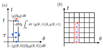
Figure 1: (a) The Berry connection $A^{(t)}$ in the temporal gauge and (b) its lattice analogue Fukui et al. (2005).

The discussion up to this point is general and applicable for both with/without edges.

Now let us consider a system with edges by imposing the open boundary condition. In this case, the twist of the hopping $e^{-{\mathrm{i}}\theta/L_{x}}$ is gauged out by the many body gauge transformation

$${\cal U}(\theta) = \prod_{j=1}e^{-{\mathrm{i}}\theta n_{j}(j-j_{0})/L_{x}},\quad j_{0}=L_{x}/2,$$

which operates for the fermion operator as ${\cal U}c_{j}{\cal U}^{\dagger}=e^{{\mathrm{i}}\theta j/L_{x}}c_{j}$ and we have $|g(\theta)\rangle={\cal U}|g_{0}\rangle$ where $|g_{0}\rangle$ is a snap shot ground state of the hamiltonian $H(0,t)$. Then noting that $A_{t}=\langle g|\partial_{t}g\rangle=\langle g_{0}|\partial_{t}g_{0}\rangle$ is $\theta$ independent and $A_{\theta}=\langle g_{0}|{\cal U}^{\dagger}\partial_{\theta}{\cal U}|g_{0}\rangle$, the Berry connection in the temporal gauge for the system with edges is

$$A^{(t),{\rm e}}_{\theta} = -{\mathrm{i}}\big{[}P(t)-P(0)\big{]},\ P(t)=\sum\nolimits_{j}x_{j}\rho_{j}(t)$$

where $\rho_{j}(t)=\langle g_{0}(t)|n_{j}|g_{0}(t)\rangle$, $x_{j}=\frac{j-j_{0}}{L_{x}}$ and $P(t)$ is the CM. Now we have the pumped charge as

$$\Delta Q_{[t_{a},t_{b}]} = P(t_{b})-P(t_{a}).$$

Note that this is only well defined for a system with boundaries. We also stress that the CM derived here is distinct from the Zak phase for infinite systems. We assume $P(t)$ is a CM measured for the snap shot ground state in contact with a particle reservoir, that is, the system is specified by the chemical potential $\mu$ and the temperature is sufficiently low. It should be also distinguished from the CM of the time dependent wave function $\sum_{j}x_{j}\langle G(t)|n_{j}|G(t)\rangle,$ which is recently observed in real experiments Nakajima et al. (2015); Lohse et al. (2015); Wang et al. (2013). Even though the fermi energy is in the bulk gap, when the one particle energy of the edge state coincides to the fermi energy, the many body gap of the snap shot hamiltonian necessarily closes and the edge state becomes suddenly occupied/unoccupied (See Fig.2). This sudden change of the snap shot ground state causes singularities (discontinuities) in ${{P}}$ since the edge state is spatially localized and its contribution to the normalized CM is $\pm 1/2$ in the limit $L_{x}\to\infty$. This is inevitable since topologically non trivial ground state is associated with the edge states passing through the gap. Then labeling the gap closing time’s by $t_{i}$’s ($t_{i}<t_{i+1}$, $i=1,2,\cdots$) and dividing the period into the time intervals without the singularities (patch-working in the the time domain), the total pumped charge in a single period $T$ is given as

$$\Delta{Q^{\rm e}} = \sum_{i}\int_{t_{i}^{+}}^{t_{i+1}^{-}}dt\,\partial_{t}P(t)=\sum_{i}\big{[}P(t_{i+1}^{-})-P(t_{i}^{+})\big{]}$$

$$= -\sum_{i}\big{[}P(t_{i}^{+})-P(t_{i}^{-})\big{]}=-\sum_{i}\Delta P(t_{i}),$$

where $t_{i}^{\pm}\equiv t_{i}\pm 0$ and $\Delta{P}(t_{i})\equiv P(t_{i}^{+})-P(t_{i}^{-})$ is a discontinuity of the CM at $t_{i}$. Also we used the periodicity of the CM in the adiabatic limit $P(t+T)=P(t)$, which follows from the periodicity of the hamiltonian $H(t+T)=H(t)$. This simple expression can be understood as a bulk-edge correspondence in time domain. We put ”${\rm e}$” to mark the expression for the system with edges. Note here that $P$ is only well defined with edges and can not be defined for a system with periodic boundary condition. Depending on the position of the edge state that cuts the fermi energy and the way it does, this discontinuity is determined as

$$\Delta P(t_{i}) = \left\{\begin{array}[]{ccc}-1/2&\text{Right}:&\text{become\ unoccupied}\\ +1/2&\text{Right}:&\text{become\ occupied}\\ +1/2&\text{Left}:&\text{become\ unoccupied}\\ -1/2&\text{Left}:&\text{become\ occupied},\end{array}\right.$$

where “Right” implies the edge state is localized near the boundary $j=L_{x}$ and the “Left” is for the edge states near the boundary $j\sim 0$.

Since the pair of the discontinuity coincides to the winding of the corresponding edge state energy around the “hole” (that corresponds to the energy gap) on the Riemann surface Hatsugai (1993a), total discontinuity is given by the winding number $I_{M}$ of the edge states

$$\sum_{i}\Delta P(t_{i}) = -I_{M},\qquad\Delta{Q^{\rm e}}=I_{M},$$

where we assume that the fermi energy is in the $M$-th energy gap from below. This algebraic definition of the winding number is only possible for the Harper equation, that is, only for special form of the $v_{j}(t)$. However the relation is generically justified by defining the winding number $I_{M}$ as the number of paired edge states with suitable sign depending on the direction of the crossing of the spectral flow with the fermi energy. This is a modified Laughlin argument Laughlin (1981) which is widely used for the topological number of edge states for various topological phasesHatsugai (1993a); Kane and Mele (2005); Qi et al. (2006). Since the total number of particles is conserved, the gapless times $t_{i}$’s that correspond to the (dis)appearance of the edge state are paired (irrespective to the position). It guarantees the quantization of the total pumped charge $\Delta Q^{\rm e}$ as an integer since even number of additions of $\pm 1/2$ is an integer. It is a consequence of the local $U(1)$ gauge symmetry as the Laughlin argument, but has sharp contrast to the QHE in which contribution of the edge states to the Hall conductance are always integers in the process of a unit flux penetration, since the right/left edge states are always paired on the Fermi surface. This $\pm 1/2$ contribution can be understood as a fractionalization of electrons into massive Dirac fermionsNiemi and Semenoff (1983); Hatsugai et al. (1996).

Also counting the topological number with discontinuities here should be compared with the counting of the singularities of the $\eta$-invariant for the Atiyah-Patodi-Singer index theorem Atiyah et al. (1976); Alvarez-Gaumé et al. (1985). Here we have clarified the close inter-relation between the topological nature of the discontinuities and local $U(1)$ gauge symmetry. This is not just a math but plays a crucial role in the recent experimentsNakajima et al. (2015); Lohse et al. (2015).

As an example, we calculated the CM, $P(t)$, numerically for $\phi=2/7$ and $L_{x}=1750$ and $L_{x}=350$. By the clear finite size effects, the discontinuities deviates from $\pm 1/2$ but approaches to the quantized values $\pm 1/2$ by the limit $L_{x}\to\infty$. In this case, we have $\Delta Q^{\rm e}=-2$.

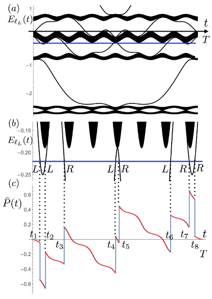
Figure 2: (a) One particle spectrum $E_{\ell_{L}}(t)$ and the fermi energy (blue line): $t_{x}=t_{y}=1$, $\phi=2/7$ and $L_{x}=1750$ (350). (b) Enlarged spectrum near the fermi energy. (c) The CM, $P(t)$, with edges by numerical calculation. $\Delta{{P}}(t_{i})=-0.499503(-0.4954)$, $0.496542(0.487094)$, $0.498412(0.494115)$, $0.497435(0.491092)$, $0.497435(0.491092)$, $0.498412(0.494115)$, $0.496542(0.487094)$, and $-0.499503(-0.4954)$ for $i=1,\cdots,8$. $\sum_{i}\Delta{{P}}(t_{i})=1.98577(1.9538)$.

Note that although the total pumped charge is governed by the discontinuity $\sum_{i}\Delta{{P}}(t_{i})$ due to the edge states, pumped charge is not carried by singularities caused by the edge states. The charge is still carried by the bulk as we explain below. This is the bulk-edge correspondence in the topological pumping. As one can see in Fig.2, the charge is pumped in the intervals between the singularities (red lines), which is the bulk contribution. Even though the system has boundaries, the effects of the edges are negligible for the bulk state since the one particle state of the bulk is extended and the amplitude near the boundaries is vanishing in the limit $L_{x}\to\infty$.

Although the CM is ill-defined for bulk (both for a periodic/infinite system), the pumped charge is well-defined as discussed by Thouless　Thouless (1983). As for an infinite system, the one particle state is given by the Bloch state $\psi_{j,\ell_{L}}\propto e^{{\mathrm{i}}k_{x}j}u_{j}(k_{x})$.

Now let $|g^{(t)}\rangle$ be a many body ground state of the snap shot hamiltonian in the temporal gauge. Assuming the fermi energy is in the $M$-th gap, one has

$$A^{(t),{\rm b}}_{\theta} = \langle g^{(t)}|\partial_{\theta}g^{(t)}\rangle=\int_{0}^{\Delta k}\frac{dk_{x}}{2\pi}\,a^{(t)}_{k_{x}},$$

$$a^{(t)}_{k_{x}} = {\rm Tr}_{M}{\cal A}^{(t)}_{k_{x}},\ {\cal A}^{(t)}_{k_{x}}=u^{\dagger}\partial_{k_{x}}u,\ u=(\bm{u}_{1},\cdots,\bm{u}_{M}),$$

where the limit $L_{x}\to\infty$ is taken and additional gauge condition $a^{(t)}_{t}={\rm Tr}_{M}u^{\dagger}\partial_{t}u=0$ is imposed. Also we put “${\rm b}$” to specify that it is purely from bulk. By using the gauge invariant form of the temporal gauge,

$$a^{(t)}_{k_{x}}(k_{x},t) = a_{k_{x}}(k_{x},t)-\partial_{k_{x}}\int_{0}^{t}d\tau\,a_{t}(k_{x},\tau)-a_{k_{x}}(k_{x},0),$$

the time derivative of $A^{(t),{\rm b}}_{\theta}$ is written by the field strength of the Bloch state, $b=\partial_{k_{x}}a_{t}-\partial_{t}a_{k_{x}}=-\partial_{t}a^{(t)}_{k_{x}}$. Now the bulk contribution of the pumped charge between the time period $[t_{a},t_{b}]$ is written asThouless (1983)

$$\Delta Q^{\rm b}_{[t_{a},t_{b}]} = {\mathrm{i}}\int_{t_{a}}^{t_{b}}dt\partial_{t}A^{(t),{\rm b}}_{\theta}=\frac{1}{2\pi{\mathrm{i}}}\int_{t_{a}}^{t_{b}}dt\int_{0}^{\Delta k}{dk_{x}}b(k_{x},t).$$

It implies that ${\mathrm{i}}\partial_{t}A^{(t),{\rm b}}_{\theta}$ is an effective CM of the bulk, even though the CM itself is not well defined.

To demonstrate the contribution of the pumping with edges is from the bulk, let us define a pumped charge between the time period $[t_{a},t_{b}]$ by compensating (skipping) the singularities from the edges as

$$\Delta Q^{\rm e}_{[t_{a},t_{b}]} = {{P}}(t_{b})-{{P}}(t_{a})-\int_{t_{a}}^{t_{b}}d\tau\,\sum_{i}\Delta{{P}}(t_{i})\delta(\tau-t_{i}).$$

This is a bulk contribution to the CM for the system with edges. According to the consideration here, we expect this bulk contribution $\Delta Q^{\rm e}_{[t_{a},t_{b}]}$ asymptotically approaches to $\Delta Q^{\rm b}_{[t_{a},t_{b}]}$ in the large system. We have numerically evaluated them for $\phi=2/7$ and shown in Fig.3. They show clear coincidence within numerical errors, indicating the relation between the bulk and the edges.

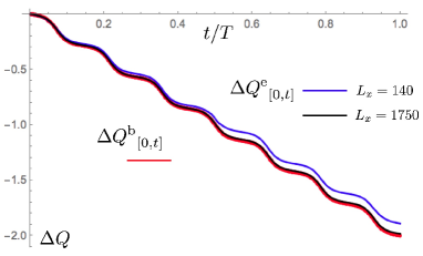
Figure 3: Pumped charge between the time interval $[0,t]$. The red line is by the bulk (Bloch states) $\Delta Q^{\rm b}_{[0,t]}$. The shifted pumped charge $\Delta{Q^{\rm e}}_{[0,t]}$’s are shown for $L_{x}=140$ (blue) and $L_{x}=1750$ (black) lines. The parameters are the same as Fig.2.

The pumped charge by bulk in a cycle is given by the Chern number $C_{M}$ Thouless (1983) of the Berry connection $a_{\mu}$ as $\Delta Q^{\rm b}=\Delta Q^{\rm b}_{[0,T]}=C_{M}$. Now we have established the physical bulk-edge correspondence in the topological pumping as

$$\Delta Q^{\rm e} = \Delta Q^{\rm b}$$

that gives the relation between the two topological invariants as was also shown in the QHE as

$$I_{M} = C_{M}.$$

It guarantees quantization of the Chern number $C_{M}$, since $I_{M}$ due to the singularities of edge states is quantized by definition.

Generically the bulk-edge correspondence is for the manybody state and the bulk and the edge can not be separated. Without gapped bulk, edge states are not well defined. We put a stress on that in the present pumping of the non interacting system, the manybody state is constructed from the one particle states which are classified into the bulk(unnormalizable) and the edge(localized). Then the contributions to the pumped charge are also clearly separated (Fig.3).

To describe the topological pumping by the CM, one necessarily needs to use a system with edges in contact with a particle reservoir. As we have established here, the pumped charge of the system with edges is carried by the bulk not by the edge states and the CM observed in the cold atom experiments $P_{{\rm exp}}(t)=\sum_{j}x_{j}\langle G(t)|n_{j}|G(t)\rangle$ is described by the bulk. Still the quantization of the pumped charge is governed by the edge states where the edge states induce discontinuities in the CM in the adiabatic limit. Even though the CM shows singularities in the adiabatic limit, these singularities can not be observed in realistic experiments in cold atoms, since the appearance of the edge states at the fermi energy necessarily implies the breakdown of the adiabaticity. As in an realistic experiment with finite speed pumping, the many body wave function approximately remains unchanged passing through the gapless point, that is, the bulk is adiabatic but the edge states is well described by the sudden approximation. It causes excitation across the gap, which eventually results in accumulation/depletion of the surface charges after one cycle. These two conditions, as the bulk is adiabatic and the edge is sudden, are conflicting requirements, if one requires both limits rigorously. Then in the experiment, it may not be easy to observe exact quantization of the pumped charge, especially for cases with high Chern numbers. We have also confirmed consistency of the argument by a direct numerical integration of the Liouville$-$von Neumann equation for the density matrix.

We thank stimulating discussions on the topological pump with Y. Takahashi, S. Nakajima and M. Lohse. The work is supported in part by KAKENHI from JSPS (Nos.26247064, 25400388,16K13845).

References

- Thouless (1983) D. J. Thouless, Phys. Rev. B 27, 6083 (1983).
- Nakajima et al. (2015) S. Nakajima, T. Tomita, S. Taie, T. Ichinose, H. Ozawa, L. Wang, M. Troyer, and Y. Takahashi, Nature Physics 12, 296-300 (2016), arXiv:1507.02223 .
- Lohse et al. (2015) M. Lohse, C. Schweizer, O. Zilberberg, M. Aidelsburger, and I. Bloch, Nature Physics 12, 350–354 (2016), arXiv:1507.02225 .
- Halperin (1982) B. I. Halperin, Phys. Rev. B 25, 2185 (1982).
- Laughlin (1981) R. B. Laughlin, Phys. Rev. B 23, 5632 (1981).
- Hatsugai (1993a) Y. Hatsugai, Phys. Rev. B 48, 11851 (1993a).
- Hatsugai (1993b) Y. Hatsugai, Phys. Rev. Lett. 71, 3697 (1993b).
- Wen (1989) X. G. Wen, Phys. Rev. B 40, 7387 (1989).
- Thouless et al. (1982) D. J. Thouless, M. Kohmoto, P. Nightingale, and M. den Nijs, Phys. Rev. Lett. 49, 405 (1982).
- Kane and Mele (2005) C. L. Kane and E. J. Mele, Phys. Rev. Lett. 95, 146802 (2005).
- Bernevig et al. (2006) B. A. Bernevig, T. L. Hughes, and S.-C. Zhang, Science 314, 1757 (2006).
- Kitaev (2001) A. Y. Kitaev, Physics-Uspekhi 44, 131 (2001).
- Ryu and Hatsugai (2002) S. Ryu and Y. Hatsugai, Phys. Rev. Lett. 89, 077002 (2002).
- Qi et al. (2006) X.-L. Qi, Y.-S. Wu, and S.-C. Zhang, Phys. Rev. B 74, 045125 (2006).
- Schulz-Baldes et al. (2000) H. Schulz-Baldes, J. Kellendonk, and T. Richter, Journal of Physics A: Math. and General 33, L27 (2000).
- Graf and Porta (2013) G.Graf and M.Porta, Comm. Math. Phys 324, 851 (2013).
- Haldane and Raghu (2008) F. D. M. Haldane and S. Raghu, Phys. Rev. Lett. 100, 013904 (2008).
- Wang et al. (2008) Z. Wang, Y. D. Chong, J. D. Joannopoulos, and M. Soljačić, Phys. Rev. Lett. 100, 013905 (2008).
- Hafezi (2014) M. Hafezi, Phys. Rev. Lett. 112, 210405 (2014).
- Prodan and Prodan (2009) E. Prodan and C. Prodan, Phys. Rev. Lett. 103, 248101 (2009).
- Kane and Lubensky (2014) C. L. Kane and T. C. Lubensky, Nat Phys 10, 39 (2014).
- Kariyado and Hatsugai (2015) T. Kariyado and Y. Hatsugai, Sci. Rep. 5, 18107 (2015).
- Dalibard et al. (2011) J. Dalibard, F. Gerbier, G. Juzeliūnas, and P. Öhberg, Rev. Mod. Phys. 83, 1523 (2011).
- Mancini et al. (2015) M. Mancini, G. Pagano, G. Cappellini, L. Livi, M. Rider, J. Catani, C. Sias, P. Zoller, M. Inguscio, M. Dalmonte, and L. Fallani, Science 349, 1510 (2015).
- Fukui et al. (2005) T. Fukui, Y. Hatsugai, and H. Suzuki, J. Phys. Soc. Jpn. 74, 1674 (2005).
- Wang et al. (2013) L. Wang, M. Troyer, and X. Dai, Phys. Rev. Lett. 111, 026802 (2013).
- Niemi and Semenoff (1983) A. J. Niemi and G. W. Semenoff, Phys. Rev. Lett. 51, 2077 (1983).
- Hatsugai et al. (1996) Y. Hatsugai, M. Kohmoto, and Y.-S. Wu, Phys. Rev. B 54, 4898 (1996).
- Atiyah et al. (1976) M. F. Atiyah, V. K. Patodi, and I. M. Singer, Math. Proc. Camb. Phil. Soc. 79, 71 (1976).
- Alvarez-Gaumé et al. (1985) L. Alvarez-Gaumé, S. D. Pietra, and G. Moore, Annals of Physics 163, 288 (1985).