Critical fragmentation properties of random drilling: How many random holes need to be drilled to collapse a wooden cube?

Abstract

A solid wooden cube fragments into pieces as we sequentially drill holes through it randomly. This seemingly straightforward observation encompasses deep and nontrivial geometrical and probabilistic behavior that is discussed here. Combining numerical simulations and rigorous results, we find off-critical scale-free behavior and a continuous transition at a critical density of holes that significantly differs from classical percolation.

The connectivity of a solid block of material strongly depends on the density of defects. To systematically study this dependence one must find an experimental way to create defects inside the solid. For example, in 2D one can simply punch holes in a sheet and measure the physical properties of the remaining material. But in 3D, inducing localized defects is not simple. One conventional solution consists in perforating the material by drilling holes or laser ablation from the surface Simon and Ihlemann (1996); Nolte et al. (1997).

In a table-top experiment, we start with a solid cube of wood and plot on each face a square-lattice mesh of $L$ by $L$ cells. Initially, the cube has no holes. Sequentially, for each one of three perpendicular faces, we randomly choose one square-cell and drill a hole having a radius of $1/\sqrt{2}$ cell lengths to the other side of the cube. We repeat this process iteratively until the entire structure collapses into small pieces and the bottom and top part of the cube are no longer connected. The first row of Fig. 1(a)-(d) shows the result of the drilling process of a real cube with edge length 6 cm (manufactured from 2 cm thick plates of medium-density fiberboard (MDF)), where holes were drilled with a diameter of 1 cm. As the drilling proceeds, pieces get disconnected and eventually the entire structure collapses.

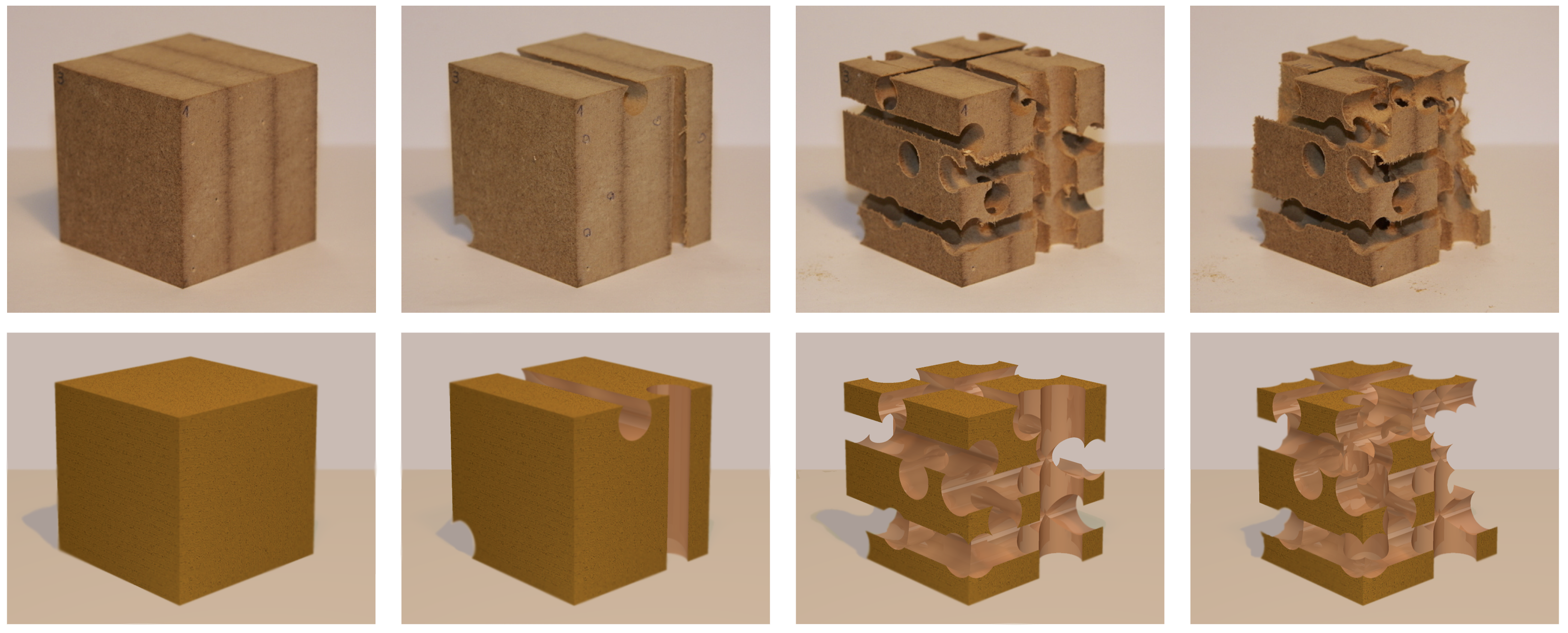
(a)               (b)               (c)               (d)

Figure 1: (color online) Cube drilling. The upper row shows photos of the experimental setup; the lower panels are the corresponding numerical results. The faces of the cube are divided with a square-lattice mesh of linear size $L=6$, such that each face can be drilled $L^{2}=36$ times. From left to right, (a) – (d), the number of drilled holes per face are (a) 0, (b) 1, (c) 6, and (d) 8. From our numerical results for the position of the transition in the thermodynamic limit (see main text), one estimates that around $13$ holes need to be drilled for the cube to disconnect.

Numerically, we start with a three-dimensional cubic lattice of $L^{3}$ sites and fix three perpendicular faces. A fraction $1-p$ square-cells on each face is randomly selected and all sites along the line perpendicular to that face are removed (second row of Fig. 1). Thirty years ago, Y. Kantor Kantor (1986) numerically studied this model on lattices of up to $10^{6}$ sites and concluded that the critical fragmentation properties of this model are in the same universality class as random percolation Stauffer (1979); Stauffer and Aharony (1994); Grimmett (1999). Here, we combine rigorous results and large-scale numerical simulations, considering lattices three orders of magnitude larger in size, to show that this is not the case. Removing entire rows at once induces strong long-range directional correlations and the critical behavior departs from random percolation. Also remarkably, while in random fragmentation power-law scaling is solely observed around the critical threshold, here we find it in an entire off-critical region. These findings suggest that long-range directional correlations lead to a rich spectrum of critical phenomena which need to be understood. Possible implications for other complex percolation models are discussed in the conclusions.

Threshold. The average total number of drilled holes is $3(1-p)L^{2}$ and the asymptotic probability that a site in the bulk is not removed is $p^{3}$. We first measure the threshold $p_{c}$ at which the cube collapses for different lattice sizes, up to $L=1024$, using different estimators of the transition point, as discussed in the Supplemental Material SM . Extrapolating the data to the limit $L\to\infty$, gives $p_{c}=0.6339\pm 0.0005$, consistent with the value estimated by Kantor using Monte Carlo renormalization group techniques Kantor (1986) (see Supplemental Material SM ). This threshold is larger than the two-dimensional square-lattice percolation threshold ($p_{2D}$) Ziff (2011); Jacobsen (2014) and smaller than the cubic root of the one for the three-dimensional simple cubic lattice Wang et al. (2013).

Static exponents. We consider the fraction $P_{\infty}$ of sites in the largest cluster of connected sites (see Supplemental Material for more data of $P_{\infty}(p)$ and of other observables SM ). $P_{\infty}$ is the standard order parameter in percolation identifying the transition from a disconnected to a globally connected state. For the drilling model, the situation will turn out to be more complicated. Figure 2(a) shows a double-logarithmic plot of the order parameter, rescaled by a power of the lattice size $P_{\infty}L^{\beta/\nu}$ as function of the distance to the transition $\lvert p-p_{c}\rvert L^{1/\nu}$. Based on finite-size scaling analysis Stauffer and Aharony (1994), we find that the critical exponent of the order parameter is $\beta=0.52\pm 0.04$, and the inverse of the correlation length exponent is $1/\nu=0.92\pm 0.01$ (see Supplemental Material). We note that both $\beta$ and $\nu$ are different from the corresponding values for 2D and 3D classical percolation. However, somehow surprisingly, the exponent ratio $\beta/\nu=0.50\pm 0.04$ is within error bars the same as for 3D percolation. Thus, while the fractal dimension of the largest cluster (given by $d_{f}=d-\beta/\nu$) is consistent with the one for 3D percolation, the larger value of $\beta$ (compared to 3D percolation) implies that the transition from the connected to the disconnected state is less abrupt (see also Supplemental Material). We consider next the behavior of the second moment of the cluster size distribution $M_{2}^{\prime}$, excluding the contribution of the largest cluster. As shown in Fig. 2(b), the finite-size scaling analysis gives that the susceptibility critical exponent is $\gamma=2.3\pm 0.1$. We note that our results for the static critical exponents are within error bars consistent with the scaling relation $2\beta+\gamma=d\nu$ (for $d=3$).

(a)

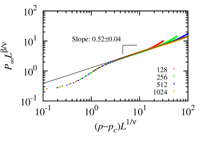
(b)

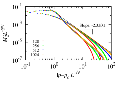
Figure 2: (color online) (a) Double-logarithmic plot of the rescaled order parameter $P_{\infty}L^{\beta/\nu}$ as function of the scaling variable $(p-p_{c})L^{1/\nu}$ for different lattice sizes $L$. The linear part has a slope of $\beta=0.52\pm 0.04$, consistent with $\beta/\nu$ being the same as for three-dimensional percolation, but with a different exponent $1/\nu=0.92$. The present value of $\beta$ is different from the two-dimensional one $\beta=5/36\approx 0.139$ Stauffer and Aharony (1994); Smirnov and Werner (2001) and the one in three dimensions, $\beta\approx 0.417$ Deng and Blöte (2005). (b) Double-logarithmic plot of the rescaled second moment $M_{2}^{\prime}L^{-\gamma/\nu}$, with $\gamma/\nu=2.0452$, as function of the scaling variable $|p-p_{c}|L^{1/\nu}$, with $1/\nu=0.92$, for different lattice sizes $L$. The solid black line is a guide to the eye with slope $-2.3$. The two sets of data points correspond to the sub-critical ($p<p_{c}$) and super-critical ($p>p_{c}$) regions.

Dynamical exponents. The transport properties of the largest cluster at the critical threshold, $p_{c}$, are intimately related to dynamical critical exponents and they can be measured by quantifying three sets of sites in the largest cluster Herrmann et al. (1984). First, we consider the so-called red sites. A site is considered a red site if its removal would lead to the collapse of the largest cluster . The red sites form a fractal set of fractal dimension $d_{\mathrm{RS}}=0.92\pm 0.07$ (see Fig. 3), which is compatible with the inverse of the correlation length exponent $\nu$ that we obtained from the finite-size scaling analysis in Fig. 2, $d_{\mathrm{RS}}=1/\nu$, as predicted by Coniglio for classical percolation Coniglio (1989). However the value of $d_{\mathrm{RS}}=1/\nu$ for the drilling transition is very different from the classical 3D percolation result $1/\nu=1.1437\pm 0.0006$ Deng and Blöte (2005). Figure 3 also shows that the shortest path connecting the top and bottom sides of the largest cluster is a fractal of fractal dimension $d_{\mathrm{SP}}=1.30\pm 0.05$. Finally, the backbone of the largest cluster between its bottom and top ends is defined as the set of sites that would carry current if a potential difference is applied between the cluster ends (also known as bi-connected component). The backbone fractal dimension is determined as $d_{\mathrm{BB}}=2.12\pm 0.08$, which is larger than in classical 3D percolation, where ${d_{\mathrm{BB}}=1.875\pm 0.003}$ Herrmann et al. (1984); Rintoul and Nakanishi (1994); Deng and Blöte (2004). Qualitatively, an increase in the backbone fractal dimension is compatible with a simultaneous decrease in the shortest path fractal dimension, since both correspond to a more compact backbone, similar to what is observed in long-range correlated percolation Prakash et al. (1992); Schrenk et al. (2013). Thus, although the fractal dimension of the largest cluster is similar in both classical percolation and drilling, the internal structure of the largest cluster is significantly different. This implies that transport and mechanical properties of the largest cluster follow a different scaling.

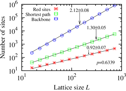
Figure 3: (color online) Number of sites in the backbone of the spanning cluster, length of its shortest path (chemical distance), and red sites in the backbone, measured at $p=p_{c}=0.6339$, as function of the lattice size $L$. Considering the local slopes of the data, we obtain the following fractal dimensions: ${d_{\mathrm{BB}}={2.12\pm 0.08}}$, ${d_{\mathrm{SP}}={1.30\pm 0.05}}$, and ${d_{\mathrm{RS}}={0.92\pm 0.07}}$. The fractal dimension of the red sites is, within error bars, compatible with the value ${1/\nu\approx 0.915}$, found from the finite size scaling behavior of the $p_{c}$ estimators (see Fig. S1), and the relation $d_{\mathrm{RS}}=1/\nu$ Coniglio (1989). Here, $d_{\mathrm{BB}}$ is larger than in classical three-dimensional percolation, where ${d_{\mathrm{BB}}=1.875\pm 0.003}$ Herrmann et al. (1984); Rintoul and Nakanishi (1994); Deng and Blöte (2004), while $d_{\mathrm{SP}}$ is smaller than the classical value ${d_{\mathrm{SP}}=1.3756\pm 0.0006}$ Zhou et al. (2012). The solid lines are guides to the eye. To extract the fractal dimensions, we analyzed the local slopes as proposed in Ref. Grassberger (1999). Results are averages over at least ${5\times 10^{3}}$ samples.

Cluster shape. Given the highly directional nature of the drilling process, we analyze the symmetry of the different clusters. In particular, we consider them as rigid bodies, consisting of occupied sites at fixed relative positions, and look at the eigenvalues and eigenvectors of their inertia tensors Rudnick and Gaspari (1987); Mansfield and Douglas (2013). The numerical results show that, when compared to classical percolation clusters, the drilling transition clusters are more anisotropic, their orientations being mainly aligned along the direction of the cube edges (see Supplemental Material for quantitative details SM ).

We now give a rigorous argument for the existence of asymmetric clusters in drilling percolation. Fix some $p\in(p_{2D},p_{c})$, where $p_{2D}\approx 0.5927<p_{c}$ is the critical threshold for $2D$ site percolation. Consider a lattice size $L_{X}\times L_{Y}\times L_{Z}$ with $L_{X}=L_{Y}=L$ and $L_{Z}=e^{L}$ and take a square domain $A$ in its base with side length $k=\sqrt{c_{0}\log(L)}$ where $c_{0}$ is a positive constant that is smaller than $-\left[\log{(p(1-p))}\right]^{-1}$. Say that the event $\mathcal{S}(A)$ occurred if, along the $z$-direction, no point inside $A$ is drilled but all points on its boundary are. For large $L$, this event happens with probability at least ${L}^{c_{0}\log{(p(1-p))}}$. Consider also two rectangles $R_{x}$ and $R_{y}$ in the $(x,z)$ and $(y,z)$-planes, respectively, aligned with $A$. These rectangles have base length $k$ and height $\exp\{c_{1}k\}$, where $c_{1}$ is an arbitrary positive constant smaller than the correlation length for two-dimensional percolation with parameter $p$. The event $\mathcal{R}_{x}$ (respectively $\mathcal{R}_{y}$) indicates the existence of a path crossing $R_{x}$ (respectively $R_{y}$) from bottom to top that has not been drilled in the $y$ (respectively $x$) direction. By our choice of $c_{1}$, $\mathcal{R}_{x}$ and $\mathcal{R}_{y}$ have positive probability (uniformly over $k$), i.e. there exists a $\delta>0$ such that $P(\mathcal{R}_{x})\geq\delta$. In addition, if $\mathcal{S}(A)$ occurs, then there exists a cluster spanning $A\times[0,e^{c_{1}k}]$ from bottom to top and whose projection into the $(x,y)$-plane does not extend beyond $A$. Thus the probability of finding a cluster of radius $k$ and height $e^{c_{1}k}$ is bounded from below by the probability that there exists a square $A$ along the diagonal $x=y$ for which $\mathcal{S}(A)\cap\mathcal{R}_{X}\cap\mathcal{R}_{Y}$ occurs, which is greater than

$$\begin{split}&1-(1-\delta^{2}L^{c_{0}\log{[p(1-p)]}})^{L(c_{0}\log{L})^{-1/2}}\\ &\geq 1-\exp(-c_{0}^{-1/2}\delta^{2}L^{1+c_{0}\log{[p(1-p)]}}\log(L)^{-1/2})\ \ ,\end{split}$$

which converges to unity as $L$ increases. This shows that one expects to have clusters extremely aligned along the $z$ axis, as numerically observed (see for example Fig. S15 of the Supplemental Material SM ). In fact, the same argument can be straightforwardly extended to explain the alignment along the $x$ and $y$ directions, as also observed.

Spanning probability. To understand the properties of the drilling transition in terms of global connectivity, we consider the spanning probability $\Pi(p)$, defined as the probability to have at least one cluster including sites from the top and bottom of the lattice, at a given value of the control parameter $p$. Figure 4 shows the spanning probability below the threshold $\Pi(p=0.63)$, for different lattice aspect ratios. The lattice size is ${L_{X}\times L_{Y}\times L_{Z}}$ with ${L_{X}=L_{Y}}$ and ${L_{Z}=rL_{X}}$ and the spanning probability is measured in the $z$-direction. At the drilling transition, $p=p_{c}$, the spanning probability approaches a constant for large lattice sizes (see Supplemental Material, Fig. S9), similar to what is observed for classical percolation Cardy (1992); Smirnov (2001). By contrast, for values of $p$ between $p_{2D}$ and $p_{*}$, the numerical results suggest a power-law decay of the spanning probability with $L_{Z}$, where the exponent increases with the aspect ratio $r$. For fixed $L_{X}$, it decays exponentially with $r$ (see inset of Fig. 4).

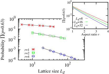
Figure 4: (color online) Main plot: Spanning probability $\Pi$, at ${p=0.63<p_{c}}$, as function of the lattice size $L_{Z}$, for different aspect ratios $r$. Solid black lines are guides to the eye with slopes, $-0.26$, $-0.58$, and $-1.22$, for ${r=1}$, $2$, and $4$. The inset shows the same probability as function of the aspect ratio $r$, for different fixed lattice sizes $L_{X}$. Results are based on at least $10^{7}$ samples.

It is possible to establish rigorously the off-critical power-law decay of $\Pi(p)$, modifying the argument for the existence of anisotropic clusters presented above. Specifically, we can show that $\Pi(p)\geq L_{X}^{-\theta}$, where $\theta=\theta(p,r)>0$, for any fixed $r>0$ and $p\in(p_{2D},p_{c})$. For that, let $B$ be the diagonal band $\{(x,y);|x-L_{X}/2|\leq\alpha n\log(L_{X}/n)$, $|x-y|<2n\}$ in the center of the $(x,y)$-face of the cube, where $\alpha$ and $n$ are constants setting the length and width, respectively. Let us say that the event $\mathcal{B}$ occurred if $B$ is free of holes in the $(x,y)$ plane i.e. if no sites in $B$ are drilled in the $z$-direction. Also say that the event $\mathcal{C}$ occurred if there exists a path $\sigma$ starting at height $z=0$ and finishing at height $z=L_{Z}$ whose projection into the $(x,y)$-plane is contained in $B$ and whose projection into the $(x,z)$-plane ($(y,z)$-plane) consists of sites that have not been drilled in the $y$-direction ($x$-direction). As discussed in detail in the Supplemental Material SM , for well chosen values of $\alpha$ and $n$ the probability of the event $\mathcal{C}$ is bounded from below by a constant not depending on $L_{X}$. Furthermore $\mathcal{B}$ and $\mathcal{C}$ are independent events. Since their joint occurrence implies the existence of a cluster including sites from the bottom and the top of the lattice, we conclude that

$$\begin{split}\Pi(p)&\geq P[\mathcal{B}\cap\mathcal{C}]=P[\mathcal{B}]P[\mathcal{C}]\\ &\geq\exp\{-c_{2}\alpha\,n\log(L_{X})\}c_{3}\geq{L_{X}}^{-\theta}\ \ ,\end{split}$$

where $c_{2}$, $c_{3}$, and $\theta$ are positive constants that depend on $p$.

The above argument also shows the existence of anisotropic clusters, sharpening the numerical results presented before. For $p<p_{2D}$, one has $\Pi(p)\sim e^{-c_{4}L_{X}}$, similarly to what happens for uncorrelated random percolation, where $c_{4}$ also depends on $p$. This is due to the fact that the projection of a path spanning the lattice into at least one of the coordinate planes is a path that spans the corresponding face, which has exponentially small probability in $L_{X}$, due to the classical exponential decay of connectivity in the subcritical phase Menshikov (1986); Aizenman and Barsky (1987).

Conclusion. We find unexpected critical behavior when sequentially drilling holes through a solid cube until it is completely fragmented. At the critical density of drilled holes, a continuous transition is observed in a different universality class than the one of random percolation. We also numerically observe off-critical scale-free behavior that we can justify for a wide range of densities of holes using rigorous arguments. This model is a representative of more complex percolation models where sites are removed in a strongly correlated manner Araújo et al. (2014); Hilário and Sidoravicius ; Liu et al. (2015). Examples are models where the set of removed sites is given by randomized trajectories, such as the so called Pacman and interlacement percolation models proposed to study the relaxation at the glass transition Pastore et al. (2013), enzyme gel degradation Abete et al. (2004) and corrosion Sznitman (2009, 2010), as well as percolation models for distributed computation Coppersmith et al. (1993); Winkler (2000). Other examples are percolation models explicitly introduce strong directional correlations as in the removal of cylinders Tykesson and Windisch (2012) and different variants of the four-vertex model Pete (2008). It would be interesting to explore up to which degree these models are in the same universality class or share common features.

While the fractal dimension of the largest fragment is consistent with the one of random percolation, all the other critical exponents are different. This has practical implications as the connectivity and transport properties do change considerably close to the threshold of connectivity. For example, we find the exponent of the order parameter to be substantially larger than for usual percolation which implies that the drilling transition is less abrupt. Since sites are removed along a line, it is necessary to remove more sites to produce the same effect in the largest fragment. We also find that, compared to usual percolation, the fractal dimension of the backbone is larger and the one of the shortest path is smaller, corresponding to a more compact backbone and therefore enhanced conductivity properties.

See pages 1,2 of drilling_SM.pdf See pages 1,3 of drilling_SM.pdf See pages 1,4 of drilling_SM.pdf See pages 1,5 of drilling_SM.pdf See pages 1,6 of drilling_SM.pdf See pages 1,7 of drilling_SM.pdf See pages 1,8 of drilling_SM.pdf See pages 1,9 of drilling_SM.pdf