Effects of Gene-Environment and Gene-Gene Interactions in Case-Control Studies: A Novel Bayesian Semiparametric Approach

Abstract

Present day bio-medical research is pointing towards the fact that virtually almost all diseases are manifestations of complex interactions of genetic susceptibility factors and modifiable environmental conditions. Cognizance of gene-environment interactions may help prevent or detain the onset of complex diseases like cardiovascular disease, cancer, type2 diabetes, autism or asthma by adjustments to lifestyle.

In this regard, we extend the Bayesian semiparametric gene-gene interaction model of ? to detect not only the roles of genes and their interactions, but also the possible influence of environmental variables on the genes in case-control studies. Our model also accounts for the unknown number of genetic sub-populations via finite mixtures composed of Dirichlet processes, which are related to each other through a hierarchical matrix-normal structure, incorporating gene-gene and gene-environment interactions. An effective parallel computing methodology, developed by us harnesses the power of parallel processing technology to increase the efficiencies of our conditionally independent Gibbs sampling and Transformation based MCMC (TMCMC) methods.

Applications of our model and methods to simulation studies with biologically realistic case-control genotype datasets obtained under five distinct set-ups of gene-environment interactions action yield encouraging results in each case. We followed these up by application of our ideas to a real, case-control based genotype dataset on early onset of myocardial infarction. Beside being in broad agreement with the reported literature on this dataset, the results obtained give some interesting insights to the differential effect of gender on MI.
Keywords: Case-control study; Dirichlet process; Gene-gene and gene-environment interaction; Matrix normal; Parallel processing; Transformation based MCMC.

1 Introduction

Although many people tend to classify the cause of a disease as either genetic or environmental, only a few diseases like Huntington’s Disease(HD) or GM2 gangliosidosis have so far been identified as purely genetic disorders. As indicated by many epidemiological studies, a different effect of a genotype is often observed on disease risk in persons with different environmental exposures (See ?, ?). Also there may be multiple genes which interact with each other to cause a disease only when an environmental factor passes a given threshold, implying thereby that presence of a risk allele may not be exposing all individuals to the same risk.

? and ?, point out that estimation of only the separate contributions of genes and environment to a disease, ignoring their interactions, will lead to incorrect estimation of the proportion of the disease (the “population attributable fraction”) that is explained by the genes, the environment, and their joint effect.

Study of gene-environment interaction is important to the field of pharmacogenetics also, since the efficacy and side-effects of some medications can vary depending on an individual’s genotype (see ?). Hence, extensive study of gene-environment interactions through sophisticated statistical modelling is necessary to devise new methods of disease prevention, detection and intervention.

Gene-environment interaction is often conceptualized as genetic control of sensitivity to different environments (?). According to ? (see also ?) gene-environment interaction is defined as “a different effect of an environmental exposure on disease risk in persons with different genotypes”. As genes are the fundamental units of change in an environmental response system, in order to model the gene-environment interaction effectively, it is important to understand the mechanism through which genes and environment interact together to bring about a physiological change in an individual. An environmental exposure could trigger a physiological change in a number of ways. Exposure to certain environmental stimuli may directly or indirectly alter the epigenome of an individual. Exposure to mutagens like high doses of x-ray or nuclear radiation, smoking etc. can enter into the body through tissues and directly interfere with the DNA sequence or replication mechanism. Some environmental stimuli may affect DNA indirectly by altering transcription factors and hence changing the expressions of certain genes. Many gene-gene interactions have been shown to be started by some environmental exposure. For example, excessive alcohol intake has been shown to suppress TACE gene, which then activates less MTHFR, resulting in reduced folate metabolism, causing depression.

Although the study of gene-environment interaction has become essential to the understanding of the aetiology of almost every disease, very little success has so far been achieved in this field. This want of success may be attributed to many causes like inadequacy of models incorporating the complex mechanism through which genes and environment may affect a disease risk (?). Indeed, given the complexity involved in the gene-environment interactions, no simple linear or additive relationship alone can model the relationship effectively. According to ? and ?, although statistical definition of gene environment interaction may lack clear biological interpretations, quantification of biological interaction should be based on statistical concepts of interaction. Furthermore, inadequacy of data regarding environmental exposure of individuals and stratified population structure are also important factors impeding success of the existing methods in this field. Association tests based on a pooled set of genetically diverse subpopulations (i.e., having differences in allele frequencies across subpopulations) may result in extremely inflated rates of false positives (see ?).

The above discussion points towards the fact that the widely-used log-linear models (see, for example, ?, ?, ?, ?, ?, ?, ?) are perhaps not quite adequate for modeling complex gene-gene and gene-environment interactions. Moreover, such models consider quite restrictive and ad-hoc association structures for simplifying computation and only attempt to test whether or not the interaction is present without being able to quantify the strength of the interaction. Uncertainty regarding unknown number of subpopulations are also not generally accounted for in the existing interaction models.

Our Bayesian hierarchical mixture model framework is aimed at incorporating all the aforementioned desirable mechanisms through which gene-environment interaction, along with the isolated effects of genes and their interactions may affect an individual’s risk of being affected by a disease, taking into account the fact that the underlying population may be stratified in nature. Since the number of sub-populations is not usually known, one must coherently and carefully account for the uncertainty associated with the unknown number of sub-populations. An additional feature of our model is learning about the number of underlying genetic sub-populations.

Because of dependence on environmental variables, our Bayesian semiparametric model comprises Dirichlet process based finite mixture models even at the individual subject level, in addition to genetic and case-control status. The mixtures share a complex dependence structure between themselves through suitable hierarchical matrix-normal distributions, suitably taking account of the dependence induced by the environmental variable. To detect the roles of genes, environment, gene-gene and gene-environment interactions, we extend the gene-gene interaction model and the associated Bayesian hypotheses testing methods of ? (henceforth, BB), and for the purpose of computation we develop a powerful parallel Markov chain Monte Carlo (MCMC) algorithm which exploits the conditional independence structures inherent in our Bayesian model, and combines the efficiencies of our Gibbs sampling method associated with the mixtures and Transformation based MCMC (TMCMC) of ?.

The rest of our paper is structured as follows. We introduce our proposed Bayesian semiparametric gene-environment interaction model in Section 2. In Section 3 we extend the Bayesian hypothesis testing procedures proposed in BB to learn about the roles of genes, environmental variables and their interactions in case-control studies. In Section 4 we demonstrate the validity of our model and methods with successful applications to five biologically realistic simulated data sets associated with five different set-ups. We also analysed a case-control type myocardial infarction data set obtained from dbGap with our model and methods, the results of which we report and discuss in detail in Section 5. As we point out, our results broadly agree with and in some cases contrast the existing results on this data set. Finally, we summarize our work with concluding remarks in Section 6. Further details are provided in the supplement, whose sections and figures have the prefix “S-” when referred to in this paper.

2 A new Bayesian semiparametric model for gene-gene and gene-environment interactions

2.1 Case-control genotype data

For $s=1,2$ denoting the two chromosomes, let $x^{s}_{ijkr}=1/0$ indicate respectively the presence and absence of the minor allele at $r$-th locus of the $j$-th gene for the $i$-th individual belonging to the $k$-th group of case/control, where $k=0,1$, with $k=1$ denoting case; $i=1,\ldots,N_{k}$; $r=1,\ldots,L_{j}$ and $j=1,\ldots,J$; let $N=N_{1}+N_{2}$. Let $\boldsymbol{E}_{i}$ denote a set of environmental variables associated with the $i$-th individual. In what follows, we model this case-control genotype data, along with the information on the environmental variables using our Bayesian semiparametric model, described in the next few sections.

2.2 Mixture models based on Dirichlet processes

Let $\mathbf{x}_{ijkr}=(x^{1}_{ijkr},x^{2}_{ijkr})$ represent the genotype at the $r$-th locus of the $j$-th gene for the $i$-th individual belonging to the $k$-th group of case/control, and let $\boldsymbol{X}_{ijk}=(\mathbf{x}_{ijk1},\mathbf{x}_{ijk2},\ldots,\mathbf{x}_{ijkL_{j}})$ denote the genotype information of the $i$-th individual of the $k$-th group at all the $L_{j}$ loci corresponding to the $j$-th gene. We assume that for every triplet $(i,j,k)$, $\boldsymbol{X}_{ijk}$ have the mixture distribution

$$[\boldsymbol{X}_{ijk}]=\sum_{m=1}^{M}\pi_{mijk}\prod_{r=1}^{L_{j}}f\left(\mathbf{x}_{ijkr}|p_{mijkr}\right),$$ (2.1)

where $f\left(\cdot|p_{mijkr}\right)$ is the Bernoulli mass function given by

$$f\left(\mathbf{x}_{ijkr}|p_{mijkr}\right)=\left\{p_{mijkr}\right\}^{x^{1}_{ijkr}+x^{2}_{ijkr}}\left\{1-p_{mijkr}\right\}^{2-(x^{1}_{ijkr}+x^{2}_{ijkr})},$$ (2.2)

and $M$ denotes the maximum number of mixture components possible.

Allocation variables $z_{ijk}$, with probability distribution

$$[z_{ijk}=m]=\pi_{mijk},$$ (2.3)

for $i=1,\ldots,N_{k}$ and $m=1,\ldots,M$, allow representation of (2.1) as

$$[\boldsymbol{X}_{ijk}|z_{ijk}]=\prod_{r=1}^{L_{j}}f\left(\mathbf{x}_{ijkr}|p_{z_{ijk}ijkr}\right).$$ (2.4)

Following ?, BB, we set $\pi_{mijk}=1/M$, for $m=1,\ldots,M$, and for all $(j,k)$.

Letting $\boldsymbol{p}_{mijk}=\left(p_{mijk1},p_{mijk2},\ldots,p_{mijkL_{j}}\right)$ denote the vector of minor allele frequencies at the $L_{j}$ loci of the $j$-th gene for the $i$-th individual of the $k$-th group of case/control corresponding to the $m$-th subpopulation (note that the vector depends upon the chromosomes through the respective genes), we next assume that

$$\boldsymbol{p}_{1ijk},\boldsymbol{p}_{2ijk},\ldots,\boldsymbol{p}_{Mijk} \stackrel{{\scriptstyle iid}}{{\sim}}\boldsymbol{G}_{ijk};$$ (2.5)

$$\boldsymbol{G}_{ijk} \sim\mbox{DP}\left(\alpha_{ijk}\boldsymbol{G}_{0,ijk}\right),$$ (2.6)

where $\mbox{DP}\left(\alpha_{ijk}\boldsymbol{G}_{0,ijk}\right)$ stands for Dirichlet process with expected probability measure $\boldsymbol{G}_{0,ijk}$ having precision parameter $\alpha_{ijk}$. We specify the base probability measure $\boldsymbol{G}_{0,ijk}$ as follows: for $m=1,\ldots,M$ and $r=1,\ldots,L_{j}$,

$$p_{mijkr}\stackrel{{\scriptstyle iid}}{{\sim}}\mbox{Beta}\left(\nu_{1ijkr},\nu_{2ijkr}\right),$$ (2.7)

under $\boldsymbol{G}_{0,ijk}$. Coincidences among $\boldsymbol{P}_{Mijk}=\left\{\boldsymbol{p}_{1ijk},\boldsymbol{p}_{2ijk},\ldots,\boldsymbol{p}_{Mijk}\right\}$, which occur with positive probability, is the property of the DP based mixture models that we exploit to learn about the actual number of mixture components.

The associated Polya urn distribution of $\boldsymbol{P}_{Mijk}$ can be derived by marginalizing over $\boldsymbol{G}_{ijk}$:

$$\left[\boldsymbol{p}_{mijk}|\boldsymbol{P}_{Mijk}\backslash\{\boldsymbol{p}_{mijk}\}\right]\sim\frac{\alpha_{ijk}}{\alpha_{ijk}+M-1}\boldsymbol{G}_{0,ijk}\left(\boldsymbol{p}_{mijk}\right)+\frac{1}{\alpha_{ijk}+M-1}\sum_{m^{\prime}\neq m=1}^{M}\delta_{\boldsymbol{p}_{m^{\prime}ijk}}\left(\boldsymbol{p}_{mijk}\right),$$ (2.8)

where $\delta_{\boldsymbol{p}_{m^{\prime}ijk}}(\cdot)$ denotes point mass at $\boldsymbol{p}_{m^{\prime}ijk}$. This scheme is useful for constructing an efficient Gibbs sampling strategy for simulating the mixtures conditional on the other parameters, embedded in a parallel MCMC strategy that we devise, bypassing the infinite-dimensional random measure $\boldsymbol{G}_{ijk}$.

Coincidences among the mixture components associate the triplets $(i,j,k)$ to different mixtures with varying number of components. Indeed, the genotype distributions of any two individuals $i$ and $i^{\prime}$ arising from a given sub-population with the same gene indexed by $j$ but with different case-control status, are likely to be different, so that $(i,j,k=0)$ and $(i^{\prime},j,k=1)$ may correspond to different mixtures. Also, for any two genes indexed by $j$ and $j^{\prime}$, $(i,j,k)$ and $(i,j^{\prime},k)$ may correspond to different mixtures because of differences in the distribution of genotypes of genes $j$ and $j^{\prime}$ for the $i$-th individual. Furthermore, for any two individuals indexed by $i$ and $i^{\prime}$, $(i,j,k)$ and $(i^{\prime},j,k)$ are likely to be associated with different mixtures because the genotype distribution of the $j$-th gene may be affected by different environmental exposures $\boldsymbol{E}_{i}$ and $\boldsymbol{E}_{i^{\prime}}$. Thus, it seems that the Dirichlet process based mixtures realistically take account of the various genotypic sub-populations and the number of such sub-populations the data arise from.

The above ideas are similar in essence to those in BB, but note that in their case, since the environmental effect $\boldsymbol{E}_{i}$ is not considered, the mixtures were with respect to $(j,k)$ only, not with respect to $(i,j,k)$ as in our current scenario influenced by $\boldsymbol{E}_{i}$.

Following BB, we set $M$, the maximum possible number of sub-populations to be $30$ and $\alpha_{ijk}=10$ in our applications. These choices are not affected by the presence of environmental variables, and performed adequately in our Bayesian analyses.

2.3 Modeling the complex dependence structure with appropriate modeling of the parameters of $\boldsymbol{G}_{0,ijk}$

We specify the dependence structure between the genes and the environment by primarily seeing to it that the environment may act upon gene-gene interaction without affecting the marginal distributions of the genotypes of the individual genes. However, we also take into account the fact that in some cases the environmental variables may cause changes in the distributions of the genotypes. Modelling the parameters of the expected probability measure $\boldsymbol{G}_{0,ijk}$ through a relevant hierarchical matrix-normal prior helps us incorporate the complex G$\times$E, G$\times$G and also the SNP$\times$SNP effects appropriately.

2.3.1 Modeling the parameters of $\boldsymbol{G}_{0,ijk}$

We model $\nu_{1ijkr}$ and $\nu_{2ijkr}$, for each loci $r=1,\ldots,L_{j}$, in $j$-th gene, of every individual $i$, having case or control status $k$, that is for every $(i,j,k)$, as the following:

$$\nu_{1ijkr} =\exp\left(u_{jr}+\lambda_{ijk}+\mu_{jk}+\boldsymbol{\beta}^{\prime}_{jk}\boldsymbol{E}_{i}\right);$$ (2.9)

$$\nu_{2ijkr} =\exp\left(v_{jr}+\lambda_{ijk}+\mu_{jk}+\boldsymbol{\beta}^{\prime}_{jk}\boldsymbol{E}_{i}\right).$$ (2.10)

The complex dependence structure that may exist between the SNPs within a gene and between the genes has been incorporated in our model by the parameters $u_{jr}$ , $v_{jr}$ and $\lambda_{ijk}$, $\mu_{jk}$ respectively (see BB for details). Here $\boldsymbol{E}_{i}$ is the $d$-dimensional vector of continuous environmental variables for the $i$th individual. The model can be easily extended to include categorical environmental variables along with the continuous ones.

Note that, non-null $\boldsymbol{\beta}_{jk}$ indicates significant marginal effect of the environmental variable $\boldsymbol{E}$ on the $j$-th gene. In Section 2.3.2 we introduce a modeling strategy that accounts for the complex phenomenon through which gene-gene interaction gets modified under the environmental effect, even though the marginal effects of the genes remain unchanged.

2.3.2 Matrix normal prior for $\lambda_{ijk}$’s

Let $\boldsymbol{\lambda}=(\boldsymbol{\lambda}_{1},\ldots,\boldsymbol{\lambda}_{J})$, where $\boldsymbol{\lambda}_{j}=(\lambda_{1j0},\ldots,\lambda_{n_{0}j0},\lambda_{1j1},\ldots,\lambda_{n_{1}j1})$, for $j=1,\ldots,J$. Note that $\lambda_{ijk}$ is shared by every locus of the $j$-th gene of the individual indexed by $(i,k)$.

We consider the following model for $\boldsymbol{\lambda}$:

$$\boldsymbol{\lambda}\sim\mathcal{N}\left(\boldsymbol{\xi},\boldsymbol{A}\otimes\tilde{\boldsymbol{\Sigma}}\right),$$ (2.11)

where $\boldsymbol{A}$ is the $J\times J$ left covariance matrix, indicating gene-gene interaction in the absence of environmental effect, and $\tilde{\boldsymbol{\Sigma}}=\boldsymbol{\Sigma}+\phi\mathcal{E}$ is the right covariance matrix under the effect of the environmental variable $E$. Here $\phi\geq 0$, $\boldsymbol{\Sigma}$ is some positive definite matrix, and the $(i,j)$-th element of the positive definite matrix $\mathcal{E}$, associated with the environmental variable $\boldsymbol{E}$, is given by

$$\mathcal{E}_{ij}=\exp\left(-b\|\boldsymbol{E}_{i}-\boldsymbol{E}_{j}\|^{2}\right),$$ (2.12)

where $b>0$ is a smoothness parameter.

Note that $\phi=0$ indicates absence of environmental effects on gene-gene interaction. It is quite important to observe that, because of the above Gaussian assumption, even for non-zero $\phi$, which points towards indirect effect of environmental factors on the epigenome, triggering genetic interactions, the marginal genotypic distributions associated with the $J$ genes of our model remain unaffected by $\boldsymbol{E}$.

For convenience, we represent the $JN$-dimensional vector $\boldsymbol{\lambda}$ as a $J\times N$ matrix $\boldsymbol{\Lambda}$, which has the following probability density function:

$$\pi(\boldsymbol{\Lambda})=\frac{\exp\left[-tr\left\{\tilde{\boldsymbol{\Sigma}}^{-1}\left(\boldsymbol{\Lambda}-\boldsymbol{\xi}\right)^{T}\boldsymbol{A}^{-1}\left(\boldsymbol{\Lambda}-\boldsymbol{\xi}\right)\right\}\right]}{\left(2\pi\right)^{J}\left|\boldsymbol{A}\right|^{N}\left|\boldsymbol{\Lambda}\right|^{J}}.$$ (2.13)

It follows that

$$\boldsymbol{\Lambda}^{col,k}\sim\mathcal{N}_{J}\left(\boldsymbol{\xi}^{col,k},\tilde{\sigma}_{kk}\boldsymbol{A}\right),$$ (2.14)

where $\boldsymbol{\Lambda}^{col,k}$ and $\boldsymbol{\xi}^{col,k}$ are the $k$-th columns of $\boldsymbol{\Lambda}$ and $\boldsymbol{\xi}$, respectively. The covariance matrix between $\boldsymbol{\Lambda}^{col,k_{1}}$ and $\boldsymbol{\Lambda}^{col,k_{2}}$ is given by

$$cov\left(\boldsymbol{\Lambda}^{col,k_{1}},\boldsymbol{\Lambda}^{col,k_{2}}\right)=\tilde{\sigma}_{k_{1}k_{2}}\boldsymbol{A},$$ (2.15)

where $\tilde{\sigma}_{k_{1}k_{2}}$ denotes the $(k_{1},k_{2})$-the element of $\tilde{\boldsymbol{\Sigma}}$. Also,

$$\boldsymbol{\Lambda}^{row,j}\sim\mathcal{N}_{N}\left(\boldsymbol{\xi}^{row,j},a_{jj}\tilde{\boldsymbol{\Sigma}}\right),$$ (2.16)

where $\boldsymbol{\Lambda}^{row,j}$ and $\boldsymbol{\xi}^{row,j}$ are the $j$-th rows of $\boldsymbol{\Lambda}$ and $\boldsymbol{\xi}$, respectively. Further,

$$cov\left(\boldsymbol{\Lambda}^{row,j_{1}},\boldsymbol{\Lambda}^{row,j_{2}}\right)=a_{j_{1}j_{2}}\tilde{\boldsymbol{\Sigma}}.$$ (2.17)

In our applications, following BB, we choose $\boldsymbol{\xi}=\boldsymbol{0}$.

To summarize, the matrix-normal prior imposes a dependence structure between the genes through the gene-gene interaction matrix $\boldsymbol{A}$, and $\tilde{\boldsymbol{\Sigma}}$ features the direct or indirect effect of the environmental factors, on the epigenome of the individuals. The randomness associated with the matrix-normal prior on $\boldsymbol{\Lambda}$ incorporates dependence between the SNPs within a gene.

Further discussion regarding the effect of environmental variables on gene-gene interaction is provided in Section S-1 of the supplement.

2.3.3 Priors for $u_{jr}$ and $v_{jr}$

We follow BB in setting, for $j=1,\ldots,J$, $u_{jr^{\prime}}=u_{r^{\prime}}$ and $v_{jr^{\prime}}=v_{r^{\prime}}$ for $r^{\prime}=1,\ldots,L$, where $L=\max\{L_{j};~{}j=1,\ldots,J\}$, and assuming for $r^{\prime}=1,\ldots,L$,

$$u_{r^{\prime}} \stackrel{{\scriptstyle iid}}{{\sim}}N(0,1);$$ (2.18)

$$v_{r^{\prime}} \stackrel{{\scriptstyle iid}}{{\sim}}N(0,1).$$ (2.19)

See BB for the details regarding the choice of $u_{jr}$ and $v_{jr}$.

2.3.4 Priors on $\mu_{jk}$, $\boldsymbol{\beta}_{jk}$, $\boldsymbol{A}$, $\boldsymbol{\Sigma}$, $b$ and $\phi$

We put the following hierarchical priors on $\boldsymbol{\mu}=(\mu_{jk};~{}j=1,\ldots,J;~{}k=0,1)$ and $\boldsymbol{\beta}=(\boldsymbol{\beta}_{\ell};~{}\ell=1,\ldots,D)$, where $\boldsymbol{\beta}_{\ell}=(\beta_{\ell jk};~{}j=1,\ldots,J;~{}k=0,1)$:

$$\boldsymbol{\mu} \sim\mathcal{N}\left(\boldsymbol{0},\boldsymbol{A}_{\alpha}\otimes\boldsymbol{\Sigma}_{\alpha}\right)$$ (2.20)

$$\boldsymbol{\beta}_{\ell} \stackrel{{\scriptstyle iid}}{{\sim}}\mathcal{N}\left(\boldsymbol{0},\boldsymbol{A}_{\beta}\otimes\boldsymbol{\Sigma}_{\beta}\right);~{}\ell=1,\ldots,D.$$ (2.21)

For priors on $\boldsymbol{A}_{\alpha}$, $\boldsymbol{A}_{\beta}$, $\boldsymbol{\Sigma}_{\alpha}$ and $\boldsymbol{\Sigma}_{\beta}$, we first consider their respective Cholesky decompositions: $\boldsymbol{A}_{\alpha}=\boldsymbol{C}_{\alpha}\boldsymbol{C}_{\alpha}^{\prime}$, $\boldsymbol{A}_{\beta}=\boldsymbol{C}_{\beta}\boldsymbol{C}_{\beta}^{\prime}$, $\boldsymbol{\Sigma}_{\alpha}=\boldsymbol{D}_{\beta}\boldsymbol{D}_{\beta}^{\prime}$ and $\boldsymbol{\Sigma}_{\beta}=\boldsymbol{D}_{\beta}\boldsymbol{D}_{\beta}^{\prime}$. We assume that the diagonal elements of the above Cholesky factors are $iid$ $Gamma(0.01,0.01)$, that is, gamma distribution with mean 1 and variance 100. We assume the non-zero off-diagonal elements of the Cholesky factors to be $iid$ $\mathcal{N}(0,10^{2})$.

Using the same Cholesky decomposition idea, we assume that the off-diagonal elements of the Cholesky factors of $\boldsymbol{A}$ and $\boldsymbol{\Sigma}$ to be $iid$ $\mathcal{N}(0,10^{2})$, and the diagonal elements to be $iid$ $Gamma(0.01,0.01)$.

We put log-normal priors on $b$ and $\phi$, so that both $\log(b)$ and $\log(\phi)$ are normally distributed with mean zero and variance 100.

Recall that the mixtures associated with gene $j\in\{1,\ldots,J\}$, and individual $i\in\{1,\ldots,N_{k}\}$ and case-control status $k\in\{0,1\}$, are conditionally independent of each other, given the interaction parameters. This allows us to update the mixture components in separate parallel processors, conditionally on the interaction parameters. Once the mixture components are updated, we update the interaction parameters using a specialized form of TMCMC, in a single processor. A schematic representation of our model and the parallel processing algorithm is provided in Figures 2.1. Details of our parallel processing algorithm are provided in Section S-2 of the supplement.

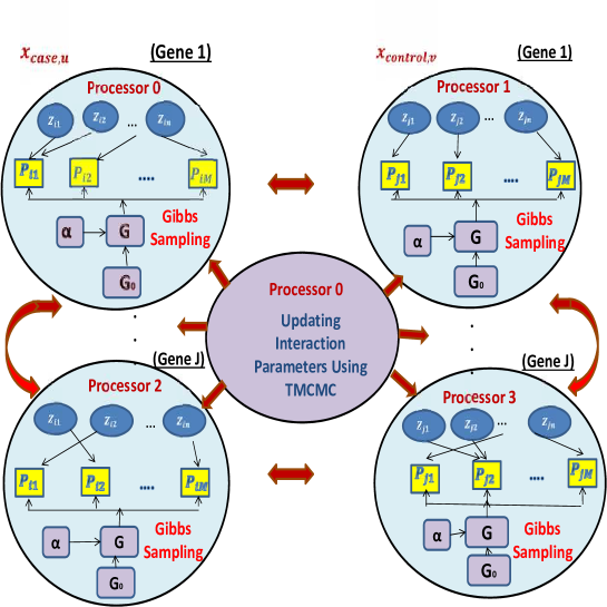
Figure 2.1: Schematic diagram for our model and parallel processing idea: The arrows in the diagram represent dependence between the variables. The ranks of the processors updating the sets of parameters in parallel using Gibbs sampling are also shown. Once the other parameters are updated in parallel, the interaction parameters are updated using TMCMC by the processor with rank zero.

3 Detection of the roles of environment, genes and their interactions in case-control studies

3.1 Formulation of appropriate Bayesian hypothesis testing procedures

In order to investigate if genes have any effect on case-control, it is pertinent to test

$$H_{01}:h_{0j}=h_{1j};~{}j=1,\ldots,J,$$ (3.1)

versus

$$H_{11}:\mbox{not}~{}H_{01},$$ (3.2)

where

$$h_{0j}(\cdot) =\prod_{i=1}^{N_{0}}\left\{\sum_{m=1}^{M}\pi_{mijk=0}\prod_{r=1}^{L_{j}}f\left(\cdot|p^{r}_{mijk=0}\right)\right\};$$ (3.3)

$$h_{1j}(\cdot) =\prod_{i=1}^{N_{1}}\left\{\sum_{m=1}^{M}\pi_{mijk=1}\prod_{r=1}^{L_{j}}f\left(\cdot|p^{r}_{mijk=1}\right)\right\}.$$ (3.4)

We shall also test, for $\ell=1,\ldots,D$; $j=1,\ldots,J$, and $k=0,1$:

$$H_{02}:\beta_{\ell jk}=0~{}\mbox{versus}~{}H_{12}:\beta_{\ell jk}\neq 0,$$ (3.5)

and

$$H_{03}:\phi=0~{}\mbox{versus}~{}H_{13}:\phi\neq 0.$$ (3.6)

The cases that can possibly arise and the respective conclusions are the following:

• If $\underset{1\leq j\leq J}{\max}~{}d(h_{0j},h_{1j})$ is significantly small with high posterior probability, then $H_{01}$ is to be accepted. If $h_{0j}$ and $h_{1j}$ are not significantly different, then it is plausible to conclude that the $j$-th gene is not marginally significant in the case-control study.

• Suppose that $H_{01}$ is accepted (so that genes have no significant role) and that $\beta_{\ell jk}$ is significant, at least for some $\ell$, $j$ and $k$, but $\phi$ is insignificant. This may be interpreted as the environmental variable $\boldsymbol{E}$ having some altering effect on the $j$-th gene, that doesn’t affect the disease status. If $\phi$ turns out to be significant, then this would additionally imply that the environmental variable $\boldsymbol{E}$ influences gene-gene interaction, but not in a way that causes the disease.

• If $H_{01}$ is rejected, indicating that the genes have significant roles to play in causing the disease, but none of the $\beta_{\ell jk}$ or $\phi$ turn out to be significant, then only genes, not $\boldsymbol{E}$, are responsible for causing the disease. In that case, the disease may be thought to be of purely genetic in nature.

• Suppose $H_{01}$ is rejected, $\beta_{\ell j0}$ and $\beta_{\ell j1}$ turn out to be significant, but that $H_{0\ell j}:\beta_{\ell j0}=\beta_{\ell j1}$ is accepted.Then although $\boldsymbol{E}$ is insignificant with respect to the marginal effect of gene $j$, it affects the disease status by triggering gene-gene interaction in some genes if $\phi$ turns out to be significant.

• If $H_{01}$ is rejected, $\beta_{\ell jk}$ is significant for some $\ell$, $j$, $k$, and $\phi$ is insignificant, then the presence of $\boldsymbol{E}$ has altering effect on some genes, which, in turn, cause the disease. In this case, since $\phi$ is insignificant, $\boldsymbol{E}$ does not seem to influence gene-gene interaction.

• If $H_{01}$ is rejected, $\beta_{\ell jk}$ is insignificant for all $\ell$, $j$, $k$, but $\phi$ is significant, then significant effect of $\boldsymbol{E}$ on altering the marginal effect of genes is to be ruled out, and one may conclude that the underlying cause of the disease is gene-gene interaction, which has been adversely affected by the environmental variable.

• If $H_{01}$ is rejected, $\beta_{\ell jk}$ is significant for some $\ell$, $j$, $k$, and $\phi$ is also significant, then the environmental variable has possibly significantly affected both the marginal and also gene-gene interaction adversely to cause the disease.

3.2 Hypothesis testing based on clustering modes

For $k=0,1$, let $i_{k}$ denote the index of the “central” clusterings of $\boldsymbol{P}_{Mijk}=\left\{\boldsymbol{p}_{1ijk},\boldsymbol{p}_{2ijk},\ldots,\boldsymbol{p}_{Mijk}\right\}$, $i=1,\ldots,N_{k}$. The concept of central clustering has been introduced by ?. Significant divergence between the two clusterings of $\boldsymbol{P}_{Mi_{0}jk=0}=\left\{\boldsymbol{p}_{1i_{0}jk=0},\boldsymbol{p}_{2i_{0}jk=0},\ldots,\boldsymbol{p}_{Mi_{0}jk=0}\right\}$ and $\boldsymbol{P}_{Mi_{1}jk=1}=\left\{\boldsymbol{p}_{1i_{1}jk=1},\boldsymbol{p}_{2i_{1}jk=1},\ldots,\boldsymbol{p}_{Mi_{1}jk=1}\right\}$, for $j=1,\ldots,J$. clearly indicates that the $j$-th gene is marginally significant. Once $i_{0}$ and $i_{1}$ are determined, we shall consider the clustering distance between $\boldsymbol{P}_{Mi_{0}jk=0}$ and $\boldsymbol{P}_{Mi_{1}jk=1}$, denoted by $\hat{d}\left(\boldsymbol{P}_{Mi_{0}jk=0},\boldsymbol{P}_{Mi_{1}jk=1}\right)$, as a suitable measure of divergence. We shall be particularly interested in

$$d^{*}=\max_{1\leq j\leq J}\hat{d}\left(\boldsymbol{P}_{Mi_{0}jk=0},\boldsymbol{P}_{Mi_{1}jk=1}\right);$$ (3.7)

In Section S-3 of the supplement we include a brief discussion of the aforementioned methodology.

BB point out that although significantly large divergence between clusterings indicate rejection of the null hypothesis, insignificant clustering distance need not necessarily provide strong enough evidence in favour of the null. In other words, even if the clustering distance is insignificant, it is important to check if the parameter vectors being compared are significantly different. In this regard, BB propose an appropriate divergence measure based on Euclidean distances of the logit transformations of the minor allele frequencies. The necessary ideas in our current context are discussed in Section S-3.1 of the supplement. In our case, in order to compute the Euclidean distance, we first compute the averages $\bar{p}_{mijk}=\sum_{r=1}^{L_{j}}p_{m,ijkr}/L_{j}$, then consider their logit transformations $\mbox{logit}\left(\bar{p}_{mijk}\right)=\log\left\{\bar{p}_{mijk}/(1-\bar{p}_{mijk})\right\}$. Then, we compute the Euclidean distance between the vectors

$$\mbox{logit}\left(\bar{\boldsymbol{P}}_{Mi_{0}jk=0}\right)=\left\{\mbox{logit}\left(\bar{p}_{1i_{0}jk=0}\right),\mbox{logit}\left(\bar{p}_{2i_{0}jk=0}\right),\ldots,\mbox{logit}\left(\bar{p}_{Mi_{0}jk=0}\right)\right\}$$

and

$$\mbox{logit}\left(\bar{\boldsymbol{P}}_{Mi_{1}jk=1}\right)=\left\{\mbox{logit}\left(\bar{p}_{1i_{1}jk=1}\right),\mbox{logit}\left(\bar{p}_{2i_{1}jk=1}\right),\ldots,\mbox{logit}\left(\bar{p}_{Mi_{1}jk=1}\right)\right\}.$$

We denote the Euclidean distance associated with the $j$-th gene by

$$d_{E,j}=d_{E,j}\left(\mbox{logit}\left(\bar{\boldsymbol{P}}_{Mi_{0}jk=0}\right),\mbox{logit}\left(\bar{\boldsymbol{P}}_{Mi_{1}jk=1}\right)\right),$$

and denote $\underset{1\leq j\leq J}{\max}~{}d_{E,j}$ by $d^{*}_{E}$.

3.3 Formal Bayesian hypothesis testing procedure integrating the above developments

In our problem, we need to test the following for reasonably small choices of $\varepsilon$’s:

$$H_{0,d^{*}}:~{}d^{*}<\varepsilon_{d^{*}}\hskip 5.69054pt\mbox{versus}\hskip 5.69054ptH_{1,d^{*}}:~{}d^{*}\geq\varepsilon_{d^{*}};$$ (3.8)

$$H_{0,d^{*}_{E}}:~{}d^{*}_{E}<\varepsilon_{d^{*}_{E}}\hskip 5.69054pt\mbox{versus}\hskip 5.69054ptH_{1,d^{*}_{E}}:~{}d^{*}_{E}\geq\varepsilon_{d^{*}_{E}};$$ (3.9)

$$H_{0,\beta_{\ell jk}}:~{}\left|\beta_{\ell jk}\right|<\varepsilon_{\ell jk}\hskip 5.69054pt\mbox{versus}\hskip 5.69054ptH_{1,\beta_{\ell jk}}:~{}\left|\beta_{\ell jk}\right|\geq\varepsilon_{\ell jk},$$ (3.10)

$$\mbox{for}~{}\ell=1,\ldots,D;~{}j=1,\ldots,J;~{}k=0,1;$$

$$H_{0,\phi}:~{}\phi<\varepsilon_{\phi}\hskip 5.69054pt\mbox{versus}\hskip 5.69054ptH_{1,\phi}:~{}\phi\geq\varepsilon_{\phi}.$$ (3.11)

If $H_{0}$ is rejected in (3.8) or in (3.9), we could also test if the $j$-th gene is influential by testing, for $j=1,\ldots,J$, $H_{0,\hat{d}_{j}}:~{}\hat{d}_{j}<\varepsilon_{\hat{d}_{j}}\hskip 5.69054pt\mbox{versus}\hskip 5.69054ptH_{1,\hat{d}_{j}}:~{}\hat{d}_{j}\geq\varepsilon_{\hat{d}_{j}}$, where $\hat{d}_{j}=\hat{d}\left(\boldsymbol{P}_{Mi_{0}jk=0},\boldsymbol{P}_{Mi_{1}jk=0}\right)$; we could also test $H_{0,d_{E,j}}:~{}d_{E,j}<\varepsilon_{d_{E,j}}\hskip 5.69054pt\mbox{versus}\hskip 5.69054ptH_{1,d_{E,j}}:~{}d_{E,j}\geq\varepsilon_{d_{E,j}}$.

To test if gene-gene interactions are significant, one may test, following BB, $H_{0,j,j^{*}}:~{}\left|\boldsymbol{A}_{jj^{*}}\right|<\varepsilon_{A_{jj^{*}}}$ versus $H_{1,j,j^{*}}:~{}\left|\boldsymbol{A}_{jj^{*}}\right|\geq\varepsilon_{A_{jj^{*}}}$, for $j^{*}\neq j$, $\boldsymbol{A}_{jj^{*}}$ being the $(j,j^{*})$-th element of $\boldsymbol{A}$. If $H_{1,j,j^{*}}$ is accepted for some (or many) $j^{*}\neq j$, then this would indicate significant interaction between the $j^{*}$-th and the $j$-th genes.

As argued in BB, here also it is easily seen that our testing procecure is equivalent to Bayesian multiple testing procedures that minimize the Bayes risk of additive “0-1” and “$0-1-c$” loss functions (see BB for the details; see also ?). Since it is well-known that Bayesian multiple tetsing methods automatically provide multiplicity control through the inherent hierarchy (see, for example, ?), separate error control is not necessary. A brief, schematic representation of the hierarchy of the hypothesis tests is shown in Figure 3.1.

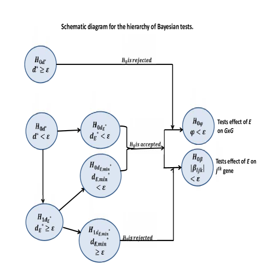
Figure 3.1: Schematic diagram for our Bayesian testing idea.

Our choices of the $\varepsilon$’s are based on the idea of null model introduced in BB. In a nutshell, we first specify an appropriate null model, which, for example, is the same model as ours but with $\boldsymbol{A}$ and $\tilde{\boldsymbol{\Sigma}}$ set to identity matrices to reflect the null hypotheses of “no interaction” and the same mixture distributions under cases and controls for each gene for no genetic effect. From the null model thus specified, we then generate case-control genotype data and fit our general Bayesian model to this “null data” and set $\varepsilon$ to be the $55$-th percentile of the relevant posterior distribution. The rationale and details of this procedure are provided in BB (particularly in Section S-7 of their supplement)

4 Simulation studies

For simulation studies, we first generate biologically realistic genotype data sets under stratified population with known G$\times$G and G$\times$E set ups from the GENS2 software of ?. We consider simulation studies in $5$ different true model set-ups: (a) presence of gene-gene and gene-environment interaction, (b) absence of genetic or gene-environmental interaction effect, (c) absence of genetic and gene-gene interaction effects but presence of environmental effect, (d) presence of genetic and gene-gene interaction effects but absence of environmental effect, and (e) independent and additive genetic and environmental effects.

As we demonstrate, our model and methodologies successfully identify the marginal effects of the genes, along with the G$\times$G and G$\times$E, and the number of sub-populations. Details are provided in Section S-4 of the supplement.

5 Application of our model and methodologies to a real, case-control dataset on Myocardial Infarction

MI (more commonly, heart attack), has been subjected to much investigation for detecting the underlying genetic causes, the possible environmental factors and their interactions. Application of our ideas to a case-control genotype dataset on early-onset of myocardial infarction (MI) from MI Gen study, obtained from the dbGaP database (http://www.ncbi.nlm.nih.gov/gap), led to some interesting insights into gene-environment and gene-gene interactions on incorporating sex as the environmental factor.

5.1 Data description

The MI Gen data obtained from dbGaP consists of observations on presence/absence of minor alleles at $727478$ SNP markers associated with 22 autosomes and the sex chromosomes of $2967$ cases of early-onset myocardial infarction, $3075$ age and sex matched controls. The average age at the time of MI was 41 years among the male cases and 47 years among the female cases. The data also consists of the sex information of the individuals, which we incorporate in our Bayesian model. The data broadly represents a mixture of four sub-populations: Caucasian, Han Chinese, Japanese and Yoruban. SNPs were mapped on to the corresponding genes using the Ensembl human genome database (http://www.ensembl.org/). However, technical glitches prevented us from obtaining information on the genes associated with all the markers. As such, we could categorize $446765$ markers out of $727478$ with respect to $37233$ genes.

For our analysis, we considered a set of SNPs that are found to be individually associated with different cardiovascular end points like LDL cholesterol, smoking, blood pressure, body mass etc. in various GWA studies published in NHGRI catalogue and augmented this set further with another set of SNPs found to be marginally associated with MI in the MIGen study (see ?). Our study also includes SNPs that are reported to be associated with MI in various other studies; see ?, ? and ?. In all, we obtained 271 SNPs. Unfortunately, only 33 of them turned out to be common to the SNPs of our original MI dataset on genotypes, which has been mapped on to the genes using the Ensembl human genome database. However, we included in our study all the SNPs associated with the genes containing the 33 common SNPs. Specifically, our study involves the genotypic information on 32 genes covering 1251 loci, including the 33 previously identified loci for $200$ individuals. We chose this relatively small number of individuals to ensure computational feasibility. However, even this data set, along with our model and prior, yielded results that are not only compatible with, but also complement the results established in the literature.

Categorization of the case-control genotype data into the four sub-populations, each of which are likely to represent several further and rather varied sub-populations genetically, implies that the maximum number of mixture components must be fixed at some value much higher than $4$. As before, we set $M=30$ and $\alpha_{jk}=10$ for every $(j,k)$, to facilitate data-driven inference.

We chose a similar set-up for the null model. That is, we chose the same number of genes and the same number of loci for each gene, the same number of cases and controls, the same value $M=30$, but $\alpha_{jk}=1.5$ for every $(j,k)$, as in our simulation studies. We use the same priors as in the real data set-up except that we set $\boldsymbol{A}$ and $\boldsymbol{\Sigma}$ to be identity matrices to ensure that the genetic interaction is not present and set the same mixture distribution under cases and controls for each gene to ensure the absence of genetic effects.

5.2 Remarks on incorporation of the sex variable in our model

In our case, $\boldsymbol{E}_{i}=E_{i}$, a one-dimensional binary variable, where $E_{i}=1$ if the $i$-th individual is male and $E_{i}=0$ if female. Hence, $\boldsymbol{\beta}_{jk}=\beta_{jk}$ is a scalar quantity. In (2.9) and (2.10) we considered the environmental variable to be continuous, but remarked that the model can be easily extended to include categorical variables. Indeed, in this case the exponentials of (2.9) and (2.10) can be thought of as binary regressions with sex as the covariate.

As regards $\mathcal{E}_{ij}$ of (2.12), we first consider $a_{0}+a_{1}E_{i}$ as a binary regression, and then write

$$\mathcal{E}_{ij}=\exp\left(-\|(a_{0}+a_{1}E_{i})-(a_{0}+a_{1}E_{j})\|^{2}\right)=\exp\left[-a^{2}_{1}(E_{i}-E_{j})^{2}\right],$$ (5.1)

with $b=a^{2}_{1}$ being the smoothness parameter. Observe that for the same sex, $\mathcal{E}_{ij}=1$ while for different sex, $\mathcal{E}_{ij}=\exp(-b)<1$.

5.3 Remarks on model implementation

We first obtain the number of parameters to be updated by TMCMC in our case; other unknowns associated with the mixtures, to be updated using Gibbs steps in parallel. Note that in our case, the interaction matrix $\boldsymbol{A}$ is of order $32\times 32=1024$, and the associated Cholesky decomposition then consists of $33\times 16=528$ parameters. Also, $\boldsymbol{\lambda}$ is a $NJ=200\times 2=400$-dimensional random vector and $\boldsymbol{\Sigma}$ is of order $N\times N=200\times 200$, so that its Cholesky decomposition consists of $201\times 100=20100$ parameters. Furthermore, $\left\{(u_{r},v_{r}):r=1,\ldots,L\right\}$, where $L=207$, consists of $2\times 207=414$ parameters, $\boldsymbol{\mu}$ and $\boldsymbol{\beta}$ consist of $64$ parameters each, and there are two more parameters $b$ and $\phi$. So, in all, there are $21572$ parameters to be updated simultaneously in a single block using TMCMC.

We implemented our parallel MCMC algorithm detailed in S-2 of the supplement on a VMware consisting of $50$ double-threaded, $64$-bit physical cores, each running at $2493.990$ MHz. In spite of the large number of parameters associated with the interaction part, our mixture of additive and additive-multiplicative TMCMC still ensured reasonable performance.

Our parallel MCMC algorithm takes about $11$ days to yield $100,000$ iterations in our aforementioned VMware machine. We discard the first $50,000$ iterations as burn-in. Informal convergence diagnostics such as trace plots exhibited adequate mixing properties of our parallel algorithm.

5.4 Results of the real data analysis

5.4.1 Effect of the sex variable

It turned out that $\varepsilon_{\phi}=1.043069$ and $P(\phi<\varepsilon_{\phi}|\mbox{Data})\approx 1$, so that $\phi$ is clearly insignificant, indicating no differential effect of sex on the genetic interactions. The posterior probabilities $P(|\beta_{1j1}-\beta_{1j0}|<\varepsilon|\mbox{Data})$ are shown in Figure 5.1. As before, $\varepsilon$ is the $55$-th percentile of the posterior distribution of $|\beta_{1j1}-\beta_{1j0}|$ under the null model. Under the 0-1 loss function, the above posterior probability exceeding $0.5$ indicates significant environmental effect on the $j$th gene. From the figure it is interesting to note that there is significant differential effect due to sex on the marginal effects of several genes although sex does not affect the genetic interactions significantly.

Figure 5.1: Index plots of posterior probabilities of no environmental effect with respect to $|\beta_{1j0}-\beta_{1j1}|<\varepsilon$, for $j=1,\ldots,32$.

5.4.2 Influence of genes and gene-gene interactions on MI based on our study

Our Bayesian hypotheses testing using the clustering metric yielded $P\left(d^{*}<\epsilon_{1}|\mbox{Data}\right)\approx 0.35202$ while that with the Euclidean distance we obtained $P\left(d^{*}_{E}<\epsilon_{2}|\mbox{Data}\right)\approx 0.51078$. In other words, it seems rather debatable whether or not the genes have significant overall effect on MI. This is in sharp contrast with the results obtained by BB where both clustering metric and Euclidean distance confirmed significant overall genetic influence on MI. However, both the posterior probabilities are substantially large, practically indicating that the genes are not very significant.

As far as testing of significance of the individual genes are concerned, it turned out that under the clustering metric, except genes $SMARCA4$, $RBMS1$, $COL4A1$, $RP11-306G20.1$, $MRAS$, $SLC22A1$, $CDKAL1$, $PCSK9$, $ADAMTS9-AS2$, and $AP006216.5$, the rest turned out to be significant, while with respect to the Euclidean metric the only insignificant genes are $AP006216.10$, $CELSR2$, $MRAS$, $PCSK9$, $OR4A48P$ and $BUD13$. The posterior probabilities of the null hypotheses (of no significant genetic influence) are shown in Figure S-3 of the supplement. The figure reveals that the posterior probabilities of no significant genetic influence, although generally did not cross $0.5$, are not adequately small to reflect very strong evidence against the null hypotheses. This is consistent with the result on overall genetic significance that we obtained.

The actual gene-gene correlations based on medians of the posterior covariances, are shown in Figure S-4 of the supplement. The color intensities correspond to the absolute values of the correlations. Consistent with the figure, all the tests on interaction turned out to support the hypotheses of no interaction.

Thus, individual genes have impact on MI but not gene-gene interactions. Moreover, the relatively weak evidences against the null suggest that external factors, in our case sex, may be playing a bigger role in explaining case-control with respect to MI. As such, given our data set of size $200$ with $77$ cases, the empirical conditional probability of a male given case is $0.3766234$, while the empirical conditional probability of a male given control is $0.504065$, indicating that with respect to our data, females seem to be more at risk compared to males. Coherency of Bayesian models in general is instrumental in reflecting this information in our inference in the way of downplaying the genes, suggesting at the same time that the only external factor, namely, sex, must have more important effect.

A detailed investigation of the disease predisposing loci detected by our model and methods, and the role of SNP-SNP interactions behind such disease predisposing loci, is carried out in Section S-5 of the supplement, and a discussion on the posterior distribution of the number of distinct mixture components is provided in Section S-6 of the supplement.

5.5 Discussion of our Bayesian methods and GWAS in light of our findings

Our results of Bayesian analysis of the MI data set demonstrate that sex plays more significant role than the genes in triggering the disease, and in particular, do not support gene-gene interaction. In these regards, our results significantly differ from those obtained by BB, who do not consider the sex variable in their model. Since as per our inference sex seems to be far more influential compared to the genes with respect to MI, there is internal consistency of our more general gene-gene and gene-environment interaction model with the gene-gene interaction model of BB. It is important to note that ? analyzed the same MI dataset using logistic regression and reached the same conclusion as ours that there is no significant gene-gene interaction. Since two completely different methods of analyses are in such strong agreement, it is pertinent to presume that the data contains enough information on the lack of gene-gene interaction. However, as we demonstrated, SNP-SNP correlations have important roles to play in determining the DPLs. These are responsible for suppression of the SNPs considered influential in the literature by implicit induction of negative correlations between Euclidean distances between cases and controls for the associated SNPs. Thus, even though the genes did not turn out to be as significant, it is clear that sophisticated nonparametric modeling of gene-gene and SNP-SNP interactions is of utmost importance.

6 Summary and conclusion

In this paper, we have extended the Bayesian semiparametric gene-gene interaction model of BB to realistically include the case of gene-environment interactions. Careful attention has been paid to the fact that in the absence of mutation, the environmental variable does not affect the marginal genotypic distributions, in spite of influencing gene-gene interaction. Needless to mention, our model considers dependence between SNPs as well to account for LD effects, in addition to gene-gene, gene-environment and dependencies between individuals. Besides, our model, via Dirichlet processes, facilitates learning about the number of genotypic sub-populations associated with the individuals and the genes, while accounting for the environmental effect at the same time.

We extend the Bayesian hypotheses testing methods introduced in BB to enable test for significances of marginal genetic and environmental effects, gene-gene interactions, effect of environment on gene-gene interaction and mutational effect. The basis for our tests are extensions of the clustering metric based tests proposed by BB to account for the environmental variables, in conjunction with the tests based on Euclidean metric. We recommended careful application of our tests based on the clustering metric, followed by re-confirmation with respect to the Euclidean metric.

On the Bayesian computational side, we propose a powerful parallel processing algorithm that takes advantage of the conditional independence structures built within our model through the Dirichlet process based mixture framework for parallelisation, and is complemented by the efficiency of TTMCMC, which updates the interaction parameters within a single processor.

We validate our model and methodologies with applications to biologically realistic datasets generated from under $5$ different set-ups characterized by different combinations and structures associated with gene-gene and gene-environment interactions. Adequate performance of our model and methods are demonstrated in every situation. Additionally, our ideas correctly captured the true number of genetic sub-populations in each case, and attempted to capture the DPL adequately even in the face of highly complex dependence structures.

We apply our model and methods to the MI Gen data set also studied by BB and because of inclusion of the sex variable, succeeded in obtaining results that are quite compatible with those reported in the literature. Although the gene-gene interactions turned out to be insignificant, the SNP-SNP correlations associated with case-control Euclidean distances facilitated understanding the mismatch of our DPL with those reported in the literature as having significant impact on MI. Interestingly, our Bayesian approach allowed us obtain insightful results even with a sample consisting of only $200$ individuals, showing the importance of building sophisticated models and prior structures, and efficient computational methods and technologies.

Supplementary Material

S-1 Further discussion regarding the effect of environmental variables on gene-gene interaction

It is important to elucidate how our above modeling strategy accounts for the G$\times$G and G$\times$E.

Recall that in our model, $\boldsymbol{A}$ represents the gene-gene interaction matrix in the absence of environmental variables, and has essentially the same interpretation as that of BB. When there is no significant environmental effect on the genes, it is pertinent to test for the significance of the elements of $\boldsymbol{A}$ (see (2.14) and (2.15) of our main manuscript), ignoring the multiplicative constants, to learn about gene-gene interactions.

However, when $\boldsymbol{E}_{i}$ affects gene-gene interactions of individual $i$, then it follows from (2.15) of our main manuscript that the relevant gene-gene covariance matrix for individual $i$ is $\tilde{\sigma}_{ii}\boldsymbol{A}$, which involves the effect of $\boldsymbol{E}_{i}$ through $\tilde{\sigma}_{ii}$.

S-2 A parallel MCMC algorithm for model fitting

Recall that the mixtures associated with gene $j\in\{1,\ldots,J\}$, and individual $i\in\{1,\ldots,N_{k}\}$ and case-control status $k\in\{0,1\}$, are conditionally independent of each other, given the interaction parameters. This allows us to update the mixture components in separate parallel processors, conditionally on the interaction parameters. Once the mixture components are updated, we update the interaction parameters using a specialized form of TMCMC, in a single processor. The details of updating the mixture components in parallel are as follows.

• Split the triplets $\left\{(i,j,k):~{}i=1,\ldots,N_{k};~{}j=1,\ldots,J;~{}k=0,1\right\}$ in the available parallel processors. For our convenience, we split the triplets sequentially into

  $$\mathcal{T}_{1}=\left\{(i,j,0):~{}i=1,\ldots,N_{0};~{}j=1,\ldots,J\right\}$$

  and

  $$\mathcal{T}_{2}=\left\{(i,j,1):~{}i=1,\ldots,N_{1};~{}j=1,\ldots,J\right\};$$

  we then parallelise updation of the mixtures associated with $\mathcal{T}_{1}$, followed by those of $\mathcal{T}_{2}$.

• During each MCMC iteration, for each $(i,j,k)$ in each available parallel processor, do the following

  1. Update the allocation variables $z_{ijk}$ by simulating from the full conditional distribution of $z_{ijk}$, given by

     $$[z_{ijk}=m|\cdots]\propto\pi_{mijk}\prod_{r=1}^{L_{j}}f\left(\mathbf{x}_{ijkr}|p_{mijkr}\right);$$ (S-2.1)

     for $m=1,\ldots,M$.

  2. Let $\left\{\boldsymbol{p}^{*}_{1ijk},\ldots,\boldsymbol{p}^{*}_{\tau_{ijk}ijk}\right\}$ denote the distinct elements in $\boldsymbol{P}_{Mijk}=\left\{\boldsymbol{p}_{1ijk},\ldots,\boldsymbol{p}_{Mijk}\right\}$. Also let $\boldsymbol{C}_{ijk}=\left\{c_{1ijk},\ldots,c_{Mijk}\right\}$ denote the configuration vector, where $c_{mijk}=\ell$ if and only if $\boldsymbol{p}_{mijk}=\boldsymbol{p}^{*}_{\ell ijk}$.

     Now let $\tau^{(m)}_{ijk}$ denote the number of distinct elements in $\boldsymbol{P}_{-Mijkm}=\boldsymbol{P}\backslash\left\{\boldsymbol{p}_{mijk}\right\}$ and let ${\boldsymbol{p}^{m}}^{*}_{\ell}=\left\{{p^{m}}^{*}_{\ell ijkr};~{}r=1,\ldots,L_{j}\right\};~{}\ell=1,\ldots,\tau^{(m)}_{ijk}$ denote the distinct parameter vectors. Further, let ${\boldsymbol{p}^{m}}^{*}_{\ell}$ occur $M_{\ell m}$ times.

     Then update $c_{mijk}$ using Gibbs steps, where the full conditional distribution of $c_{mijk}$ is given by

     $$[c_{mijk}=\ell|\cdots]\propto\left\{\begin{array}[]{ccc}q^{*}_{\ell,mijk}&\mbox{if}&\ell=1,\ldots,\tau^{(m)}_{ijk};\\ q_{0,mijk}&\mbox{if}&\ell=\tau^{(m)}_{ijk}+1,\end{array}\right.$$ (S-2.2)

     where

     $$q_{0,mijk} =\alpha_{ijk}\prod_{r=1}^{L_{j}}\frac{\beta\left(n_{1mijkr}+\nu_{1ijkr},n_{2mijkr}+\nu_{2ijkr}\right)}{\beta\left(\nu_{1ijkr},\nu_{2ijkr}\right)};$$ (S-2.3)

     $$q^{*}_{\ell,mjk} =M_{\ell m}\prod_{r=1}^{L_{j}}\left\{{p^{m}}^{*}_{\ell jkr}\right\}^{n_{1mijkr}}\left\{1-{p^{m}}^{*}_{\ell ijkr}\right\}^{n_{2mijkr}}.$$ (S-2.4)

     In (S-2.3) and (S-2.4), $n_{1mijkr}$ and $n_{2mijkr}$ denote the number of $``a"$ and $``A"$ alleles, respectively, at the $r$-th locus of the $j$-th gene of the $i$-th individual, associated with the $m$-th mixture component. In other words, $n_{1mijkr}=x^{1}_{ijkr}+x^{2}_{ijkr}$ and $n_{2mjr}=2-\left(x^{1}_{ijkr}+x^{2}_{ijkr}\right)$. The function $\beta(\cdot,\cdot)$ in the above equations is the Beta function such that for any $s_{1}>0,s_{2}>0$, $\beta(s_{1},s_{2})=\frac{\Gamma(s_{1})\Gamma(s_{2})}{\Gamma(s_{1}+s_{2})}$; $\Gamma(\cdot)$ being the Gamma function.

  3. Let ${n}^{*}_{1\ell ijkr}=\sum_{m:c_{mijk}=\ell}n_{1mijkr}$ and ${n}^{*}_{2\ell ijkr}=\sum_{m:c_{mijk}=\ell}n_{2mijkr}$. Then, for $\ell=1,\ldots,\tau_{jk}$; $r=1,\ldots,L_{j}$; $j=1,\ldots,J$ and $k=0,1$, update ${p}^{*}_{\ell ijkr}$ by simulating from its full conditional distribution, given by

     $$[{p}^{*}_{\ell ijkr}|\cdots]\sim\mbox{Beta}\left({n}^{*}_{1\ell ijkr}+\nu_{1ijkr},{n}^{*}_{2\ell ijkr}+\nu_{2ijkr}\right).$$ (S-2.5)

• During each MCMC iteration, update the interaction parameters $\left\{(u_{r^{\prime}},v_{r^{\prime}});~{}r^{\prime}=1,\ldots,L\right\}$, $\boldsymbol{\Lambda}$, $\boldsymbol{A}$ and $\boldsymbol{\Sigma}$, $\boldsymbol{A}_{\alpha}$, $\boldsymbol{A}_{\beta}$, $\boldsymbol{\Sigma}_{\alpha}$, $\boldsymbol{\Sigma}_{\beta}$, $b$, and $\phi$ in a single processor using TMCMC, conditionally on the remaining parameters. As in BB, we update these parameters using a mixture of additive and additive-multiplicative TMCMC, exploiting the Cholesky factorizations of the positive definite matrices, and updating only the non-zero elements of the respective lower triangular matrices.

S-3 Clustering metric, clustering mode, and divergence measures based on Euclidean distance

Let $C_{1}$ and $C_{2}$ denote two possible clusterings of some dataset. Let ${K_{1}}$ and $K_{2}$ denote the number of clusters of clusterings $C_{1}$ and $C_{2}$ respectively, and let $\tilde{n}_{{i}{j}}$ denote the number of units belonging to the ${i}$-th cluster of $C_{1}$ and ${j}$-th cluster of $C_{2}$, and $\tilde{n}_{00}=\sum\sum\tilde{n}_{ij}$ is the total number of units. Following ? and BB we consider the following divergence between $C_{1}$ and $C_{2}$, which has been conjectured to be a metric by ?:

$$\hat{d}(C_{1},C_{2})=\max\left\{\bar{d}(C_{1},C_{2}),\bar{d}(C_{2},C_{1})\right\},$$ (S-3.1)

where

$$\bar{d}(C_{1},C_{2}) = \left\{\tilde{n}_{00}-\sum_{{i}=1}^{K_{1}}\max_{1\leq j\leq K_{2}}\tilde{n}_{{i}{j}}\right\}\bigg{/}{\tilde{n}}_{00}$$ (S-3.2)

$$= 1-\frac{\sum_{{i}=1}^{K_{1}}\underset{1\leq j\leq K_{2}}{\max}{\tilde{n}}_{{i}{j}}}{{\tilde{n}}_{00}}.$$ (S-3.3)

Let $\mathcal{C}$ denote the set of all possible clusterings of some dataset. Motivated by the definition of mode in the case of parametric distributions, ? define that clustering $C^{*}$ as “central,” which, for a given small $\epsilon>0$, satisfies the following equation:

$$P\left(\left\{C\in\mathcal{C}:\hat{d}(C^{*},C)<\epsilon\right\}\right)=\sup_{C^{\prime}\in\mathcal{C}}P\left(\left\{C\in\mathcal{C}:\hat{d}(C^{\prime},C)<\epsilon\right\}\right).$$ (S-3.4)

Note that $C^{*}$ is the global mode of the posterior distribution of clustering as $\epsilon\rightarrow 0$. Thus, for a sufficiently small $\epsilon>0$, the probability of an $\epsilon$-neighborhood of an arbitrary clustering $C^{\prime}$, of the form $\left\{C:\hat{d}(C^{\prime},C)<\epsilon\right\}$, is highest when $C^{\prime}=C^{*}$, the central clustering.

In a set of clusterings $\left\{C^{(\ell)}:\ell=1,\ldots,L\right\}$, ? define that clustering $C^{(j)}$ as “approximately central,” which, for a given small $\epsilon>0$, satisfies the following equation:

$$C^{(j)}=\arg\max_{1\leq\ell\leq L}\frac{1}{L}\#\left\{C^{(k)};1\leq k\leq L:\hat{d}(C^{(\ell)},C^{(k)})<\epsilon\right\}.$$ (S-3.5)

The central clustering $C^{(j)}$ is easily computable, given $\epsilon>0$ and a suitable metric $d$. Also, by the ergodic theorem, as $L\rightarrow\infty$ the empirical central clustering $C^{(j)}$ converges almost surely to the exact central clustering $C^{*}$.

In our case, we shall obtain $i_{0}$ and $i_{1}$, the indices of the central clusterings associated with $\boldsymbol{P}_{Mijk=0};~{}i=1,\ldots,N_{0}$ and $\boldsymbol{P}_{Mijk=1};~{}i=1,\ldots,N_{1}$, respectively, obtained by the above method. Once $i_{0}$ and $i_{1}$ are determined, we shall consider clustering distances between $\boldsymbol{P}_{Mi_{0}jk=0}$ and $\boldsymbol{P}_{Mi_{1}jk=1}$, denoted by $\hat{d}\left(\boldsymbol{P}_{Mi_{0}jk=0},\boldsymbol{P}_{Mi_{1}jk=1}\right)$. We shall be particularly interested in (3.7). A schematic representation of our model and hypothesis testing based on the ideas of central clustering is shown in Figure S-1.

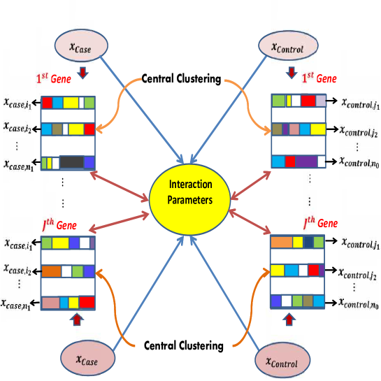
Figure S-1: Schematic diagram for our model and testing of hypothesis based on the ideas of central clustering.

S-3.1 Shortcoming of the clustering metric for hypothesis testing and a divergence measure based on Euclidean distance

BB note that when two clusterings are the same, minimizing the Euclidean distance over all possible permutations of the clusters, provides a sensible measure of divergence. In other words, for any two vectors $\boldsymbol{v}^{(1)}=\left(v^{(1)}_{1},\ldots,v^{(1)}_{K}\right)$ and $\boldsymbol{v}^{(2)}=\left(v^{(2)}_{1},\ldots,v^{(2)}_{K}\right)$ in $K$-dimensional Euclidean space, where $K>1$, BB propose the following divergence measure:

$$d_{E,\mbox{min}}\left(\boldsymbol{v}^{(1)},\boldsymbol{v}^{(2)}\right)=\min_{j_{1},\ldots,j_{K}}\sqrt{\sum_{i=1}^{K}\left(v^{(1)}_{i}-v^{(2)}_{j_{i}}\right)^{2}},$$ (S-3.6)

the minimization being over all possible permutations $(j_{1},j_{2},\ldots,j_{K})$ of $(1,2,\ldots,K)$. The above divergence is non-negative, symmetric in that $d_{E,\mbox{min}}\left(\boldsymbol{v}^{(1)},\boldsymbol{v}^{(2)}\right)=d_{E,\mbox{min}}\left(\boldsymbol{v}^{(2)},\boldsymbol{v}^{(1)}\right)$, satisfies the property $d_{E,\mbox{min}}\left(\boldsymbol{v}^{(1)},\boldsymbol{v}^{(2)}\right)=0$ if and only if $\boldsymbol{v}^{(1)}=\boldsymbol{v}^{(2)}$, and is invariant with respect to permutations of the clusters.

Since computation of $d_{E,\mbox{min}}$ involves minimization over all possible permutations, great computational burden will be incurred. BB devise a strategy based on the simple Euclidean distance $d_{E}$ (which does not require minimization over permutations), which can often avoid such computational burden. The idea is that, if the null hypothesis is accepted with respect to $d_{E}$, then this clearly implies acceptance of the null with respect to $d_{E,\mbox{min}}$, so that minimization over permutations is completely avoided. If, on the other hand, the null is rejected when tested with $d_{E}$, then one must re-test the null using $d_{E,\mbox{min}}$, which would involve dealing with permutations. In our case we compute the Euclidean distance after giving the logit transformation to the minor allele frequences. The details are provided in Section 3.2 of the main manuscript. The method of selecting appropriate $\varepsilon$’s for the hypotheses tests are provided in Section S-4 of the supplement.

S-4 Simulation studies

S-4.1 First simulation study: presence of gene-gene and gene-environment interaction

S-4.1.1 Data description

As in BB we consider two genetic factors as allowed by GENS2 and simulated 5 data sets with gene-gene and gene-environment interaction with a one-dimensional environmental variable, associated with 5 sub-populations. One of the genes consists of 1084 SNPs and another has 1206 SNPs, with one DPL at each gene. There are 113 individuals in each of the 5 data sets, from which we selected a total of 100 individuals without replacement with probabilities assigned to the 5 data sets being $(0.1,0.4,0.2,0.15,0.15)$. Our final dataset consists of 46 cases and 54 controls. Since, in our case, the environmental variable is one-dimensional, $d=1$.

S-4.1.2 Model implementation

We implemented our parallel MCMC algorithm on i7 processors by splitting the mixture updating mechanisms in 8 parallel processors, and updating the interaction parameters in a single processor. Our code is written in C in conjunction with the Message Passing Interface (MPI) protocol for parallelisation.

The total time taken to implement $100,000$ MCMC iterations, where the first $50,000$ are discarded as burn-in, is approximately 4 days. We assessed convergence informally with trace plots, which indicated adequate mixing properties of our algorithm.

S-4.1.3 Specifications of the thresholds $\varepsilon$’s using null distributions

Following the method outlined in Section 3.3.1 of our main manuscript, setting $M$, the maximum number of distinct components to be 30, and $\alpha_{ijk}=1.5$ following BB, we obtain

$\varepsilon_{d^{*}}=0.633$, $\varepsilon_{\hat{d}_{1}}=0.6$, $\varepsilon_{\hat{d}_{2}}=0.6$, $\varepsilon_{d^{*}_{E}}=18.000$, $\varepsilon_{d^{*}_{E,1}}=17.483$, $\varepsilon_{d^{*}_{E,2}}=17.249$, $\varepsilon_{\beta_{110}}=0.570$, $\varepsilon_{\beta_{120}}=0.665$, $\varepsilon_{\beta_{111}}=1.819$, $\varepsilon_{\beta_{121}}=1.106$, $\varepsilon_{\phi}=0.658$, $\varepsilon_{A_{12}}=\varepsilon_{A_{21}}=0.200$.

S-4.1.4 Results of fitting our model

The posterior probabilities $P\left(d^{*}<\varepsilon_{d^{*}}|\mbox{Data}\right)$, $P\left(\hat{d}_{1}<\varepsilon_{\hat{d}_{1}}|\mbox{Data}\right)$ and $P\left(\hat{d}_{2}<\varepsilon_{\hat{d}_{2}}|\mbox{Data}\right)$ empirically obtained from $50,000$ MCMC samples, turned out to be $0.358$, $0.334$ and $0.336$, respectively. Hence, $H_{0,d^{*}}$, $H_{0,\hat{d}_{1}}$ and $H_{0,\hat{d}_{2}}$ are rejected, suggesting the influence of significant genetic effects in the case-control study. Moreover, $P\left(d^{*}_{E}<\varepsilon_{d^{*}_{E}}|\mbox{Data}\right)$, $P\left(\hat{d}_{E,1}<\varepsilon_{\hat{d}_{E,1}}|\mbox{Data}\right)$ and $P\left(\hat{d}_{E,2}<\varepsilon_{\hat{d}_{E,2}}|\mbox{Data}\right)$ are given, approximately, by $0.460$, $0.916$ and $0.361$, respectively. That is, even though $H_{0,\hat{d}^{*}_{E,1}}$ is to be accepted, there is not enough evidence to suggest acceptance of $H_{0,\hat{d}^{*}_{E,2}}$ and $H_{0,\hat{d}^{*}_{E}}$. Thus, with respect to the “0-1” loss, the test with respect to the Euclidean-based metric is consistent with the test with respect to the clustering metric.

To check the influence of the environmental variable on the genes we compute the posterior probabilities $P\left(|\beta_{1jk}|<\varepsilon_{\beta_{1jk}}|\mbox{Data}\right)$, for $j=1,2$ and $k=0,1$. The probabilities turned out to be $0.759$, $0.253$, $1.000$ and $1.000$, respectively, showing that $\beta_{111}$ is significant. That is, the environmental variable has a significant effect on gene $j=1$. Now if gene-gene interaction is found to be significant, then the interaction of the environment and gene 1 would seem to have affected gene $j=2$ as well, so that both $H_{0,\hat{d}_{1}}$ and $H_{0,\hat{d}_{2}}$ are rejected. Hence, we now investigate the significance of gene-gene interaction.

As regards $\phi$, the corresponding posterior probability turned out to be $0.982$, indicating its insignificance. Noting that the model of ? does not have provision for any interaction terms related to our matrix $\mathcal{E}$, $\phi=0$ is the true hypothesis. The relevant posterior probability of $\boldsymbol{A}_{12}$ ($=\boldsymbol{A}_{21}$) is given by $\mbox{P}\left(\left|\boldsymbol{A}_{12}\right|<\varepsilon_{A_{12}}|\mbox{Data}\right)\approx 0.463$, which implies statistically significant gene-gene interaction under the “$0-1$” loss.

This seems to confirm the roles of genes, influenced by the environmental variable in the simulated case-control study.

Finally, the true number of sub-populations has been identified correctly by our model and methods, even though we set the maximum number of components $M$ to be $30$. All the posteriors related to the number of components have correctly concentrated around 5, the true number of components, a few of which are shown in Figure S-1.

(a) Posterior of $\tau_{110}$.

(b) Posterior of $\tau_{211}$.

(c) Posterior of $\tau_{120}$.

(d) Posterior of $\tau_{221}$.

Figure S-1: Gene-gene and gene-environment interaction: Posterior distributions of the number of distinct components.

S-4.1.5 Detection of DPL

The correct positions of the DPL, provided by GENS2, are $rs13266634$ and $rs7903146$, for the first and second gene respectively. Due to the LD effects implied by the correlated structured of our model the actual DPL need not be easy to locate. For the gene-gene interaction model of BB it has been possible to identify a relatively small set of loci which included the actual DPLs. Our current gene-gene and gene-environment interaction model is, however, much more structured due to incorporation of gene-environment dependence in addition to gene-gene dependence. In particular, since $\nu_{1ijkr}$ and $\nu_{2ijkr}$ consist of $\lambda_{ijk}$, $\mu_{jk}$ and $\boldsymbol{\beta}_{jk}$ that are shared by every locus of the $j$-th gene of the individual denoted by $(i,k)$, and because $\beta_{121}$ is significant in our example, this induces further dependence between the loci of the second gene. Because of gene-gene interaction, this also implicitly induces further dependence between the loci of the first gene. Hence, it is rather challenging to locate the DPLs in the presence of both gene-gene and gene-environmental interactions.

But in spite of the difficulties, it has been possible to segregate the DPL, albeit not as precisely as in BB. Borrowing the idea of BB, and letting $\boldsymbol{p}^{r}_{ijk}=\left\{p_{mijkr}:m=1,\ldots,M\right\}$, we declare the $r$-th locus of the $j$-th gene as disease pre-disposing if, for the $r$-th locus, the Euclidean distance $d^{r}_{j}\left(\mbox{logit}\left(\boldsymbol{p}^{r}_{i_{0}jk=0}\right),\mbox{logit}\left(\boldsymbol{p}^{r}_{i_{1}jk=1}\right)\right)$, between $\mbox{logit}\left(\boldsymbol{p}^{r}_{i_{0}jk=0}\right)$ and $\mbox{logit}\left(\boldsymbol{p}^{r}_{i_{1}jk=1}\right)$, is significantly larger than $d^{r^{\prime}}_{j}\left(\boldsymbol{p}^{r^{\prime}}_{i_{0}jk=0},\boldsymbol{p}^{r^{\prime}}_{i_{1}jk=1}\right)$, for $r^{\prime}\neq r$. We adopt the graphical method as BB.

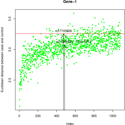
(a) Index plot for the first gene

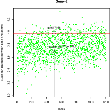
(b) Index plot for the second gene.

Figure S-2: Index plots: Plots of the Euclidean distances $\left\{d^{r}_{j}\left(\boldsymbol{p}^{r}_{i_{0}jk=0},\boldsymbol{p}^{r}_{i_{1}jk=1}\right);~{}r=1,\ldots,L_{j}\right\}$ against the indices of the loci, for $j=1$ (panel (a)) and $j=2$ (panel (b)).

The red, horizontal lines in the panels of Figure S-2 represent the cut-off value such that the points above the horizontal line are those with the highest $10\%$ Euclidean distances. The true DPLs and the SNPs which are the nearest neighbors of the true DPLs with Euclidean distances on or above the red, horizontal line are shown in the figures. It is interesting to note that even though the Euclidean distances of the true DPLs fall below the red, horizontal line (due to LD effects), they are quite close to SNPs that cross the 10% horizontal line. Thus, examination of the close neighbors of the SNPs whose Euclidean distances are high, would reveal the actual DPLs.

S-4.2 Second simulation study: no genetic or environmental effect

Here we use the same case-control genotype data set as used by BB in their second simulation study where genetic effects are absent, consisting of 49 cases and 51 controls and 5 sub-populations with the mixing proportions $(0.1,0.4,0.2,0.15,0.15)$. We use the same environmental data set generated in our first simulation study described in Section S-4.1, which is unrelated to this genotype data.

Here we obtain, from $50,000$ MCMC samples, $P\left(d^{*}<\varepsilon_{d^{*}}|\mbox{Data}\right)\approx 0.359$, $P\left(\hat{d}_{1}<\varepsilon_{\hat{d}_{1}}|\mbox{Data}\right)\approx 0.337$ and $P\left(\hat{d}_{2}<\varepsilon_{\hat{d}_{2}}|\mbox{Data}\right)\approx 0.334$. Thus, even though neither genes nor environment are responsible for the case-control status under the true, data-generating model of GENS2, still $H_{0,d^{*}}$, $H_{0,\hat{d}_{1}}$ and $H_{0,\hat{d}_{2}}$ are rejected.

However, $P\left(d^{*}_{E}<\varepsilon_{d^{*}_{E}}|\mbox{Data}\right)\approx 0.761$, so that $H_{0,d^{*}_{E}}$ is to be accepted. This also implies that there is no significant difference between the mixture models $h_{0j}$ and $h_{1j}$ for $j=1,2$. The apparent conflict between acceptance of $H_{0,d^{*}_{E}}$ and rejection of $H_{0,d^{*}}$ can be clarified as follows. Since we are considering the distance between two central clusterings, and there is a non-negligible amount of uncertainty associated with the central clustering because of relatively small sizes of case and control groups in these simulation studies, the distance between the central clusterings turn out to be larger compared to the gene-gene interaction studies carried out by BB, which did not involve distances between central clusterings. In our situation, the number of clusters remained around 5 as in the previous simulation study, but the clusters of two central clusterings associated with cases and controls turned out to have only a few common elements, thus contributing towards relatively large distance. Also, the data sets generated by GENS2 provide somewhat lesser information when fitted to our complex Bayesian nonparametric model, as compared to the data generated from our null Bayesian nonparametric model itself. This problem is further aggravated since the central clusterings themselves are subject to a (relatively large) degree of approximation, as discussed above. Consequently, the distance between central clusterings associated with the null model and the null data is somewhat lesser than that associated with the data simulated from GENS2.

Hence, here one needs to exercise caution to reach the right conclusion. Indeed, $P\left(d_{E,1}<\varepsilon_{d_{E,1}}|\mbox{Data}\right)\approx 0.713$ and $P\left(d_{E,2}<\varepsilon_{d_{E,2}}|\mbox{Data}\right)\approx 0.946$, also suggesting acceptance of $H_{0,d_{E,1}}$ and $H_{0,d_{E,2}}$. Also recall that BB obtained, for the same genotype data, the clear conclusion of acceptance of all three hypotheses $H_{0,d^{*}}$, $H_{0,\hat{d}_{1}}$ and $H_{0,\hat{d}_{2}}$, with respect to both clustering and Euclidean distances associated with their gene-gene interaction model. Thus our results with respect to the Euclidean distance is consistent with the results obtained by BB. We conclude that genes are not responsible for the case-control outcome in this study. Hence, the environmental variable has no negative influence on the genes in triggering the disease. Note that given the above conclusion, the tests involving $\beta_{\ell jk}$ and $\phi$ are rendered unimportant. As before, our model has successfully captured 5 sub-populations.

Since we model the genotype data conditionally on the case-control status, rather than modelling the case-control status directly as binary outcomes, it is not possible to infer from the above conclusion that the environmental variable is irrelevant for the case-control outcome in this study. To test whether or not the environmental variable is marginally influential, one may consider direct modelling of the case-control binary data using, say, the logistic regression on the environment, and then test significance of the environmental variable, independently of our Bayesian nonparametric model. Considering such a test, we obtain clear insignificance of the environmental variable.

S-4.3 Third simulation study: absence of genetic and gene-gene interaction effects but presence of environmental effect

In this study we consider a case-control genotype data set simulated from GENS2 where case-control status depends only upon the environmental data. The number of cases turned out to be 47 among a total of 100 individuals.

We obtain $P\left(|\beta_{1jk}|<\varepsilon_{\beta_{110}}|\mbox{Data}\right)\approx 0.998$, $P\left(|\beta_{1jk}|<\varepsilon_{\beta_{120}}|\mbox{Data}\right)\approx 1.000$, $P\left(|\beta_{1jk}|<\varepsilon_{\beta_{111}}|\mbox{Data}\right)\approx 1.000$, and $P\left(|\beta_{1jk}|<\varepsilon_{\beta_{121}}|\mbox{Data}\right)\approx 1.000$, suggesting that all $\beta_{1jk}$ are insignificant. This indicates that the environmental variable does not cause mutation of the genes. But even though genes are not responsible for the case-control outcome in this study, rather counter-intuitively we find that $P\left(d^{*}<\varepsilon_{d^{*}}|\mbox{Data}\right)\approx 0.359$, $P\left(\hat{d}_{1}<\varepsilon_{\hat{d}_{1}}|\mbox{Data}\right)\approx 0.336$ $P\left(\hat{d}_{2}<\varepsilon_{\hat{d}_{2}}|\mbox{Data}\right)\approx 0.332$, $P\left(d^{*}_{E}<\varepsilon_{d^{*}_{E}}|\mbox{Data}\right)\approx 0.236$, $P\left(\hat{d}_{E,1}<\varepsilon_{\hat{d}_{E,1}}|\mbox{Data}\right)\approx 0.548$ and $P\left(\hat{d}_{E,2}<\varepsilon_{\hat{d}_{E,2}}|\mbox{Data}\right)\approx 0.298$, all suggesting the relevance of genes in this experiment. Significant gene-gene interaction is also indicated by $P\left(\left|\boldsymbol{A}_{12}\right|<\varepsilon_{A_{12}}|\mbox{Data}\right)\approx 0.450$. It also turned out, counter-intuitively, that $P\left(\phi<\varepsilon_{\phi}|\mbox{Data}\right)\approx 0.351$, suggesting significant impact of the environmental variable on gene-gene interaction.

In an attempt to resolve this dilemma we again considered a logistic linear regression of the case-control status on the environmental variable and the (summaries of the) genes, and obtained, using the Akaike Information Criterion (AIC), the model consisting of the marginal effects of the environment and the second gene, as the best model. Thus, relevance of at least the second gene is also revealed by this simple logistic linear model.

Since gene-environment interaction is ruled out by the best logistic linear model, we re-implemented our model by setting $\phi=0$, so that the environmental variable can not have any effect on gene-gene interaction. This can be interpreted as (data based) prior information obtained from the best logistic linear model. With this prior information it then turned out that $P\left(d^{*}<\varepsilon_{d^{*}}|\mbox{Data}\right)\approx 0.358$, $P\left(\hat{d}_{1}<\varepsilon_{\hat{d}_{1}}|\mbox{Data}\right)\approx 0.340$ $P\left(\hat{d}_{2}<\varepsilon_{\hat{d}_{2}}|\mbox{Data}\right)\approx 0.317$, $P\left(d^{*}_{E}<\varepsilon_{d^{*}_{E}}|\mbox{Data}\right)\approx 0.658$, $P\left(\hat{d}_{E,1}<\varepsilon_{\hat{d}_{E,1}}|\mbox{Data}\right)\approx 0.653$ and $P\left(\hat{d}_{E,2}<\varepsilon_{\hat{d}_{E,2}}|\mbox{Data}\right)\approx 0.804$, strongly suggesting that genes are not responsible for case-control status. And, as before, all the $\beta_{\ell jk}$ turned out to be insignificant, demonstrating that the environmental variable does not have any effect on the genes. Since the best logistic linear model includes the environmental variable one may conclude on this basis that the environmental effect is the only factor responsible in this case-control experiment. Thus, our inference is consistent with the true data-generating mechanism.

S-4.4 Fourth simulation study: presence of genetic and gene-gene interaction effects but absence of environmental effect

Here we use the same genotype data set as used by BB in their first simulation study associated with genetic and gene-gene interaction effects, consisting of 41 cases and 59 controls and 5 sub-populations with the mixing proportions $(0.1,0.4,0.2,0.15,0.15)$. We use the same environmental data set generated in our first simulation study described in Section S-4.1, which is unrelated to this case-control genotype data.

Here we obtain $P\left(d^{*}<\varepsilon_{d^{*}}|\mbox{Data}\right)\approx 0.362$, $P\left(\hat{d}_{1}<\varepsilon_{\hat{d}_{1}}|\mbox{Data}\right)\approx 0.336$ $P\left(\hat{d}_{2}<\varepsilon_{\hat{d}_{2}}|\mbox{Data}\right)\approx 0.337$, $P\left(d^{*}_{E}<\varepsilon_{d^{*}_{E}}|\mbox{Data}\right)\approx 0.345$, $P\left(\hat{d}_{E,1}<\varepsilon_{\hat{d}_{E,1}}|\mbox{Data}\right)\approx 0.764$ and $P\left(\hat{d}_{E,2}<\varepsilon_{\hat{d}_{E,2}}|\mbox{Data}\right)\approx 0.317$, so that importance of genes is correctly indicated by our tests.

As for the tests related to the environmental variable, we find $P\left(|\beta_{1jk}|<\varepsilon_{\beta_{110}}|\mbox{Data}\right)\approx 0.633$, $P\left(|\beta_{1jk}|<\varepsilon_{\beta_{120}}|\mbox{Data}\right)\approx 0.647$, $P\left(|\beta_{1jk}|<\varepsilon_{\beta_{111}}|\mbox{Data}\right)\approx 1.000$, and $P\left(|\beta_{1jk}|<\varepsilon_{\beta_{121}}|\mbox{Data}\right)\approx 1.000$, meaning that all the $\beta_{\ell jk}$ are insignificant. That is, mutation is to be correctly ruled out.

That the environmental variable has no influence on gene-gene interaction is clear from the result $P\left(\phi<\varepsilon_{\phi}|\mbox{Data}\right)\approx 0.640$, which correctly suggests acceptance of the null hypotheses $\phi=0$. Also, $P\left(\left|\boldsymbol{A}_{12}\right|<\varepsilon_{A_{12}}|\mbox{Data}\right)\approx 0.423$, correctly suggesting the presence of gene-gene interaction.

To check if the environmental variable has no role to play in the case-control outcome of this study we again perform analyses based on logistic regression and obtain insignificance of the environmental variable.

S-4.5 Fifth simulation study: independent and additive genetic and environmental effects

Now we simulate a case-control genotype dataset from GENS2 where the genetic and environmental effects are independent of each other and additive. Among 100 individuals obtained, there are 57 cases.

Note that in our Bayesian model there is no provision for additivity of genetic and environmental effects. Hence this dataset is not expected to provide enough information to our Bayesian model to enable it capture the true data-generating relationships between the genes and the environmental variable. Here we obtain $P\left(d^{*}_{E}<\varepsilon_{d^{*}_{E}}|\mbox{Data}\right)\approx 0.711$, $P\left(\hat{d}_{E,1}<\varepsilon_{\hat{d}_{E,1}}|\mbox{Data}\right)\approx 0.740$ and $P\left(\hat{d}_{E,2}<\varepsilon_{\hat{d}_{E,2}}|\mbox{Data}\right)\approx 0.816$, indicating that the genes are unimportant in this study. All $\beta_{\ell jk}$ also turned out to be insignificant. However, $P\left(\phi<\varepsilon_{\phi}|\mbox{Data}\right)\approx 0.054$, suggesting that gene-gene interaction is influenced by the environmental variable. Since genetic effect turned out to be insignificant, it is clear that gene-gene interaction did not have substantial effect on the case-control data.

On conducting independent logistic regression experiments as before we find that the best AIC-based model consists of the marginal effects of the environmental variable and the first gene, along with an intercept, which is somewhat consistent with the actual data-generating model.

In summary, it seems that with respect to our Bayesian model, the additive effect has been almost wholly transformed into the environmental effect, given that the provoked gene-gene interaction did not not affect the case-control data. From the practical perspective, it seems that the environmental variable exerts much stronger influence in this case-control study compared to the genes and gene-gene interaction.

(a) Posterior probability of no genetic effect with respect to clustering metric.

(b) Posterior probability of no genetic effect with respect to Euclidean metric.

Figure S-3: Posterior probabilities of no individual genetic influence in MI study: Index plots of the posterior probabilities of the null hypotheses for (a) clustering metric and (b) Euclidean metric, for the $32$ genes.

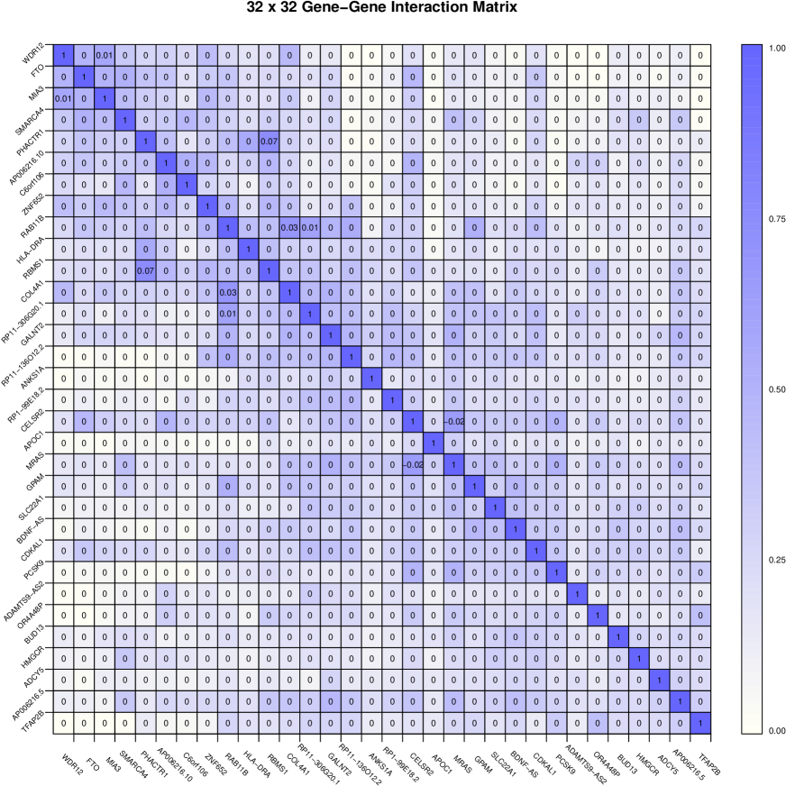
(a) Colorplot of actual posterior gene-gene interaction.

Figure S-4: Gene-gene interaction plot in MI study: Actual gene-gene interactions based on medians of the absolute values of the posterior covariances.

S-5 Disease predisposing loci detected by our Bayesian analysis

Figure S-5 shows the index plots of the posterior medians of the clustering and Euclidean distances between case and control, with respect to the corresponding genes.

(a) Clustering metric medians.

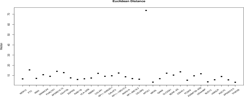
(b) Euclidean metric medians.

Figure S-5: Posterior medians of the Euclidean distances: Index plots of the posterior medians of the Euclidean distances with respect to the $32$ genes.

It is clear from the figure that in terms of the clustering metric, genes $FTO$, $PHACTR1$, $GALNT2$, $RP11-136O12.2$, $ANKS1A$ and $ADCY5$ exceed $0.66$, while $APOC1$ exceeds $70$ in terms of the Euclidean distance. The number of loci of these $7$ genes are $137$, $177$, $89$, $45$, $54$, $95$ and $1$, respectively.

After computing the averaged Euclidean distances $\left\{d^{r}_{j}\left(\mbox{logit}\left(\boldsymbol{p}^{r}_{jk=0}\right),\mbox{logit}\left(\boldsymbol{p}^{r}_{jk=1}\right)\right);~{}r=1,\ldots,L_{j}\right\}$, of the loci in each such Gene-$j$, where the averages are taken over the TMCMC samples, we single out that SNP with maximum such distance and compare this SNP, which we continue to refer to as DPL, with that SNP of Gene-$j$ which is reported in the literature as important. Our findings are reported in Figures S-6 and S-7. Since $APOC1$ consists of only one SNP ($rs4420638$), that SNP is clearly our DPL, and so this case does not present any new insight. As such, we do not display the corresponding diagram.

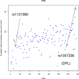
(a) DPL of $FTO$.

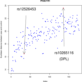
(b) DPL of $PHACTR1$.

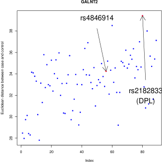
(c) DPL of $GALNT2$.

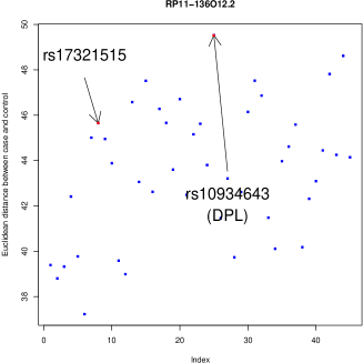
(d) DPL of $RP11-136O12.2$.

Figure S-6: Disease predisposing loci of the genes influential with respect to the clustering metric: Plots of the Euclidean distances $\left\{d^{r}_{j}\left(\mbox{logit}\boldsymbol{p}^{r}_{jk=0},\mbox{logit}\boldsymbol{p}^{r}_{jk=1}\right);~{}r=1,\ldots,L_{j}\right\}$ against the indices of the loci.

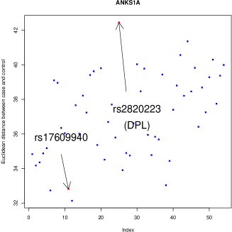
(a) DPL of $ANKS1A$.

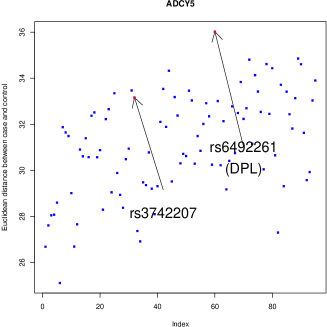
(b) DPL of $ADCY5$.

Figure S-7: Disease predisposing loci of genes influential with respect to the Euclidean metric: Plots of the Euclidean distances $\left\{d^{r}_{j}\left(\mbox{logit}\boldsymbol{p}^{r}_{jk=0},\mbox{logit}\boldsymbol{p}^{r}_{jk=1}\right);~{}r=1,\ldots,L_{j}\right\}$ against the indices of the loci.

S-5.1 Role of SNP-SNP interactions behind our obtained DPLs

Figures S-6 and S-7 show that most of the literature based SNPs have turned out to be less influential in terms of case-control Euclidean distance. BB showed that with respect to their Bayesian model it is possible to explain agreements and disagreements between the literature based SNPs and the important SNPs obtained from their model in terms of gene-gene and SNP-SNP interactions. In our case, although it turned out that gene-gene interactions are insignificant, there are still substantial SNP-SNP interactions with respect to case-control Euclidean distances. Indeed, we illustrate that such SNP-SNP correlations play important roles in this regard. Recall that $APOC1$ consisting of the singleton locus $rs4420638$, is the most influential with respect to the Euclidean metric in terms of case-control Euclidean distance. The correlation between the case-control Euclidean distances associated with the literature-cited locus $rs1121980$ of $FTO$ and $rs4420638$ of $APOC1$ is $-0.198163$, and this negative correlation with the most influential SNP is responsible for low influence of $rs1121980$ in comparison with the DPL $rs1051336$, which the correlation $-0.1162004$ with $APOC1$.

As regards $PHACTR1$, the correlation between the literature based $rs12526453$ and $rs2820223$ of $ANKS1A$ is $-0.3860316$. Since $rs2820223$ is also the DPL of $ANKS1A$, it is not at all unlikely that $rs12526453$ would turn out to be less significant because of the negative correlation. However, the correlation of the DPL of $ANKS1A$ with the DPL $rs10265116$ of $PHACTR1$ is $-0.4036174$, which is more negative than than that with the literature based SNP. To comprehend this counter-intuitive phenomenon, note that $APOC1$ exerts more positive influence on the DPL (correlation $0.3131022$) than on the literature based locus (correlation $0.279255$), so that overall the DPL seems to have more influence.

The same locus $rs2820223$ of $ANKS1A$ also exerts negative influence on $rs4846914$ of $GALNT2$, with correlation $-0.2414285$, and on $rs17321515$ of $RP11-136O12.2$, with correlation $-0.03827756$, taking away much of the influences of the aforementioned literature based loci. The correlations of the DPL of $ANKS1A$ with the DPLs of $GALNT2$ and $RP11-136O12.2$ are $-0.2182731$ and $-0.01800756$, respectively, which are larger than the correlations with the literature based SNPs. Furthermore, $APOC1$ has correlations $0.2921335$ and $0.100273$ with the DPLs of $GALNT2$ and $RP11-136O12.2$ and correlations $0.2887141$ and $0.07980527$ with the literature based SNPs, which are consistent with the order associated with the correlations with the DPL of $ANKS1A$.

On the other hand, the singleton $rs4420638$ of $APOC1$ has correlation $-0.09018503$ with the literature based $rs17609940$ of $ANKS1A$ making it somewhat less influential compared to the DPL $rs2820223$, which has correlation $-0.05074254$ with $APOC1$.

For gene $ADCY5$, the DPL $rs6492261$ and the literature based locus $rs3742207$ are somewhat close in terms of their case-control Euclidean distances. Indeed, in this case, the DPL of $ANKS1A$ has almost same positive correlations $0.02089441$ and $0.02126861$ with the DPL and the literature based SNPs of $ADCY5$. Consistent with these observations, it is seen that the correlations of $APOC1$ with these two SNPs of $ADCY5$ are $0.4463449$ and $0.453281$, respectively. These seem to provide an explanation for $rs6492261$ and $rs3742207$ to be relatively consistent with each other.

A mathematical explanation of such influences based on the interactions has been provided in BB. However, as in BB here also it is useful to remark that our above explanations, even though focussed on a very small number of genes and SNPs, may still be inadequate; indeed it is not feasible to explain precisely the complex influences the SNPs have on one another which might be responsible for the discrepancies between the DPLs that we obtained and the so-called influential SNPs cited in the literature.

S-6 Posteriors of the number of distinct mixture components

Unlike BB, under the current study the posteriors of the number of distinct components associated with all the genes turn out to be almost identical. Figure S-8, shows the posteriors of the number of distinct components associated with three of the relatively influential genes, $FTO$, $PHACTR1$ and $GALNT2$. Observe that the posteriors are almost identical for all the genes, with the mode at $5$ components, and $4$ receiving the next highest probability. Recall that in case of BB, the genes turned out to be highly significant with significant interactions among them and they were associated with different posteriors. After incorporating the environmental factor, the genes seem to play very little role in causing MI and also the posteriors of the number of distinct subpopulations associated with the genes are similar. Our results are also consistent with the four broad sub-populations composed of Caucasians, Han Chinese, Japanese and Yoruban.

(a) Posterior of $\tau_{2,0}$.

(b) Posterior of $\tau_{2,1}$.

(c) Posterior of $\tau_{5,0}$.

(d) Posterior of $\tau_{5,1}$.

(e) Posterior of $\tau_{14,0}$.

(f) Posterior of $\tau_{14,1}$.

Figure S-8: Posterior of number of components: Posterior distributions of the number of distinct components $\tau_{j,k}$ for each pair ($j,k$); j=2,5,14; $k=0,1$. The left and right panels show the posteriors associated with cases and controls, respectively.