Large Anomalous Nernst Effect in a Skyrmion Crystal

Abstract

Thermoelectric properties of a model skyrmion crystal were theoretically investigated, and it was found that its large anomalous Hall conductivity, corresponding to large Chern numbers induced by its peculiar spin structure leads to a large transverse thermoelectric voltage through the anomalous Nernst effect. This implies the possibility of finding good thermoelectric materials among skyrmion systems, and thus motivates our quests for them by means of the first-principles calculations as were employed here.

I Introduction

Thermoelectric (TE) generation, harvesting waste heat and turning it into electricity, should play an important role in realizing more energy-efficient society and overcoming the global warming. Nevertheless, it is yet to be widely used, mainly due to its still limited efficiency. There have been many studies pursueing highly efficient TE systems with a large value of figure of merit: $Z_{X}=\sigma X^{2}/\kappa$, where $\sigma$ and $\kappa$ are longitudinal electrical and thermal conductivity respectively, and $X=S\ {\rm or}\ N$ is the Seebeck or Nernst coefficient depending on whether we use the longitudinal or transverse voltage for power generation. Here we omitted labels $xx$ or $yy$ in $\sigma$ and $\kappa$ by assuming an isotropic system. Among those, our study sheds light on the anomalous effect of electrical conduction perpendicular to an electric field (anomalous Hall effect, AHE) Nagaosa et al. (2010) or to a temperature gradient (anomalous Nernst effect, ANE) Xiao et al. (2006) on TE performance, focusing on a particular contribution to the conductivity of AHE (ANE), namely the so-called intrinsic term $\sigma^{\rm int}_{xy}(\alpha^{\rm int}_{xy})$ expressed as a functional of Berry curvatureXiao et al. (2010) $\Omega({\bf k})\equiv i\langle\partial_{\bf k}u|\times|\partial_{\bf k}u\rangle$ in momentum(k) space (See the middle line of Eq.(6) in Appendix A), where $|u_{\bf k}\rangle$ is the periodic part of a Bloch state.

Systems hosting AHE/ANE are found in magnetic materials, both normal semiconductors Culcer et al. (2003) and topological insulators Chang et al. (2013). We previously studied simple models of 2D electron gas in an interface composed of those materials Mizuta and Ishii (2014, 2015). The anomalous effect on Seebeck coefficient was fairly large there, but remained rather small compared to what will be reported in this paper, which can mainly be attributed to the limited magnitude of the anomalous Hall conductivity (AHC) $\sigma^{\rm int}_{xy}\leq 1$ (The unit is taken to be $e^{2}/h$ for the AHC in 2D in this paper) there.

There have been several ideas proposed for obtaining large AHC, such as the manipulation of massive Dirac cones (each of them being the source of $\sigma^{\rm int}_{xy}=1$) by controlling parameters Fang et al. (2014), or the extention of system dimension in the normal-to-plane direction (2D to 3D) Jiang et al. (2012).

What we focus here is another one, namely, the control of real-space spin textures which are well known to induce another contribution to the AHE/ANE, often called the topological Hall/Nernst conductivityNeubauer et al. (2009) $\sigma^{T}_{xy}(\alpha^{T}_{xy})$ that also has a geometrical meaning related to $\sigma^{\rm int}_{xy}(\alpha^{\rm int}_{xy})$. In terms of Berry-phase theory Xiao et al. (2010), the emergence of topological terms in the continuum limit (spin variation scale $\gg$ atomic spacing), is an analogue of the ordinary Hall effect with the external $B$ field just replaced by spin magnetic field $B_{\rm spin}$, which is the real-space Berry curvature $\Omega({\bf R})$ itself, proportional to a quantity called spin scalar chirality $\chi_{ijk}\equiv{\bf m}_{i}\cdot{\bf m}_{j}\times{\bf m}_{k}$ reflecting the geometrical structure spanned by each spin trio $({\bf m}_{i},\ {\bf m}_{j},\ {\bf m}_{k})$. Although it should be better to treat $\sigma^{\rm int}_{xy}$ and $\sigma^{T}_{xy}$ on an equal footing, we will omit the latter (topological) term in the main part of this paper because the validity of the simple relation $B_{\rm spin}\propto\Omega({\bf R})$ is not clear for our system of rather short spin variation scale. Still, the omission can be justified within this approximation (See Appedix B for details).

Among many possible spin textures, what we target here is the so-called skyrmion crystal (SkX) phase observed even near room-temperature Yu et al. (2010), where skyrmions, particle-like spin whirls, align on a lattice. The skyrmionic systems, originally explored in nuclear physics Skyrme (1962), have been studied extensively these days in condensed matter physics as well. Typical SkX-hosting materials are some of the transition metal silicides/germanides: MnSi Mühlbauer et al. (2009), MnGe, FeGe, or heterostructures such as monolayer Fe on Ir(111) Heinze et al. (2011), in all of which the Dzyaloshinskii-Moriya term, a spin-orbit coupling effect peculiar to their inversion-asymmetric crystal structure, plays a crucial role in the emergence of skyrmions.

Regarding the AHE in skyrmionic systems, phases with a quantized AHC, i.e. $\sigma^{\rm int}_{xy}=C(e^{2}/h)$ with an integer $C$ called Chern number, have been recently predicted in the models of SkX where the conduction electron spins are exchange-coupled to the SkX either strongly Hamamoto et al. (2015) or weakly Lado and Fernández-Rossier (2015), preceded by a report of QAHE in a meron (half-skyrmion) crystalMcCormick and Trivedi (2015). In this paper we focus on the case picked out in Ref.[Hamamoto et al., 2015] because of its particularly large $\sigma^{\rm int}_{xy}$, implying the possibility of large ANE as well, thanks to the close relation between AHE and ANE Xiao et al. (2006); Miyasato et al. (2007), and that is the main point we confirmed in this study.

At the end of this section, we stress that the computational method used in our study is based on first-principles, which can be applied to the exploration of realistic materials of SkX etc. from the same perspective.

II Expressions of thermoelectric quantities

The formulae for the thermoelectric cofficients to be evaluated follow from the linear response relation of charge current: ${\bf j}=\tilde{\sigma}{\bf E}+\tilde{\alpha}(-\nabla T)$, where E and $\nabla T$ are the electric field and temperature gradient present in the sample.

Using the conductivity tensors $\tilde{\sigma}=[\sigma_{ij}]$ and $\tilde{\alpha}=[\alpha_{ij}]$, we obtain

$$\left\{\begin{array}[]{l}{\displaystyle S\equiv S_{xx}\equiv\frac{E_{x}}{\partial_{x}T}=\frac{S_{0}+\theta_{H}N_{0}}{1+\theta_{H}^{2}}\vspace{2mm}}\\ {\displaystyle N\equiv S_{xy}\equiv\frac{E_{x}}{\partial_{y}T}=\frac{N_{0}-\theta_{H}S_{0}}{1+\theta_{H}^{2}}=-S_{yx}.}\end{array}\right.$$ (1)

Here we defined $S_{0}\equiv\alpha_{xx}/\sigma_{xx},\theta_{H}\equiv\sigma_{xy}/\sigma_{xx},\ N_{0}\equiv\alpha_{xy}/\sigma_{xx}$ for a simpler notation. See Eq.(6) in Appendix A for the specific form of the conductivity tensors $\sigma$ and $\alpha$ we consider here. Throughout this paper, since our 2D system has no periodicity in $z$ direction, we discuss $\sigma_{ij}\equiv\sigma_{ij}^{2D}\equiv d\times\sigma_{ij}^{3D}$, which is independent of the film thickness $d$ and has the dimension of $e^{2}/h$ whose unit can be $\Omega^{-1}$, instead of real conductivity $\sigma_{ij}^{3D}$.

Note that the Seebeck coefficient $S_{0}$ estimated without considering Berry curvature is obtained by setting $\theta_{H}=0$ and $N_{0}=0$ in Eq. (1).

III Model

We consider a magnetic SkX on a two dimensional square lattice, with its unit cell of lattice constant $2\lambda=19.8{\mathrm{\AA}}$ containing $6\times 6$ spins, thus the atomic lattice spacing $a=2\lambda/6$ being 3.3Å. The spin configuration is equivalent to the one studied in Ref.[Hamamoto et al., 2015], i.e., the spherical coordinates of spin ${\bf m}({\bf r}_{i})$ located at site $i$ are set as $\theta_{i}=\pi(1-r_{i}/\lambda)$ for $r_{i}<\lambda$ and $\theta_{i}=0$ for $r_{i}>\lambda$, along with $\phi_{i}=\tan^{-1}(y_{i}/x_{i})+C$, where $C$ is an arbitrary constant. In order to simulate the simplest case, we assumed each spin is that of a hydrogen atom. The spin modulation in the system is shown in Fig.1.

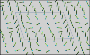
Figure 1: A view of an unit cell of $6\times 6$ SkX.

IV Computational procedure

Our calculations consist of three steps: (1) Obtain the electronic states of target SkX using OpenMX code Ozaki et al. , (2) Construct maximally localized Wannier functions (MLWF) employing Wannier90 codeMostofi et al. (2008) and finally (3) Compute from the obtained MLWF all the necessary transport quantities [tensors $\sigma$ and $\alpha$ in Eq.(6)] expressed according to the Boltzmann semiclassical transport theory, where we adopted constant-relaxation-time approximation with a fixed value of $\tau=0.1$ps .

In step(1), one s-character numerical pseudo-atomic orbital with cutoff radius of 7 bohr was assigned to each H atom. The present calculation for a non-collinear magnetic system was realized by applying a spin-constraining method Kurz et al. (2004) in the non-collinear density functional theory Kubler et al. (1972). Step(1) yielded 6$\times$6=36 non-spin-degenerate occupied bands and the equal number of unoccupied ones, among which only the former 36 bands were used in step(2) to construct MLWF and interpolated with them to calculate the conductivities. In step(3), two modules were used in Wannier90: berry module based on the formalism in Ref.[Wang et al., 2006] to compute $\sigma^{\rm int}_{xy}$ and boltzwann module introduced in Ref.[Pizzi et al., 2014] to compute $\sigma_{xx}$ and $S_{0}$, in both of which the sampling for integrations was performed on $50\times 50$ k-points. Besides these, numerical intergrations were carried out to evaluate $\alpha_{xy}$ from $\sigma_{xy}$ via Eq.(6).

The above procedure was tested, referring to Ref.[Hamamoto et al., 2015].

V Results and Discussions

V.1 Electronic structure and conductivities

First we show the obtained band structure of the 36 occupied states in Fig.2(a).

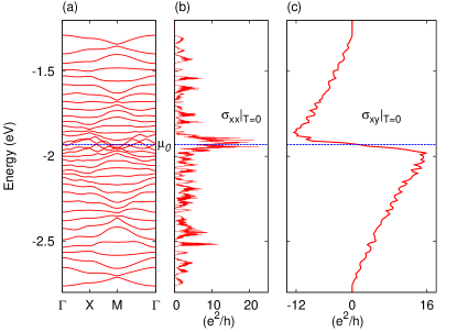
Figure 2: (a) Band structure and Fermi-level dependence of (b) longitudinal and (c) anomalous Hall conductivity of $6\times 6$ SkX. The blue dashed line indicates the $\mu_{0}$ mentioned in the main text.

We notice there that each band is well isolated from (not touching with) each other, except for the four bands around the middle energy range [-2.0, -1.9]eV, which we shall hereafter refer to as “central bands”. We also see that some neighboring bands, including the center ones, tend to converge toward M point $(0.5,\ 0.5)\pi/(2\lambda)$. Away from M point, we see some degenerate points. Regarding the dispersions, quite nice symmetry with respect to the energy $\mu_{0}\simeq-1.93$eV in the center bands also deserves close attention. Further analyses are needed in order to understand the secrets behind these interesting features.

Next, let us observe how the longitudinal conductivity $\sigma_{xx}$ and AHC at $T=0$K depend on the band filling (Fermi level) in Fig.2(b) and (c) respectively. The $\sigma_{xx}(\mu)|_{T=0}$ has a large peak in the central bands region, as can be expected from the obviously large density of states there. The $\sigma_{xx}$’s roughly symmetric variation with respect to $\mu_{0}$ (recognized when averaged over some spreaded energy) could have been anticipated intuitively from the above-mentioned symmetric band structure.

The AHC, on the other hand, shows good anti-symmetric behavior with respect to $\mu_{0}$, which is quite understandable from the combined consideration of, again, the symmetric band structure and the assumption that each of the isolated (other than the central) bands is analogous to a Landau level formed by external magnetic field which contributes AHC=1 ($e^{2}/h$) in the quantum Hall effect. The maximum absolute value of AHC is approximately 16, reached just below the central bands, while the second largest value of about 12 is located just above them. These behaviors result in the drastical change of AHC around central bands as is prominent in Fig.2(c). This very character has a strong effect on the TE properties of the system, as will be seen below.

V.2 Filling-dependence of thermoelectric properties

We will proceed to our main subjects, the TE quantities of the system, especially focusing on their electron filling dependence, which we assume to be parametrized by the chemical potential $\mu$ within the rigid band approximation. In all what is reported in this paper, the room temperature $T=300$K is assumed. The Seebeck $S$ and Nernst $N$ coefficients, the terms $S_{0},\ \theta_{H},\ N_{0}$ constituting them [Eq.(1)], and the power factors associated with each of $S$ and $N$, are shown in Fig.3(a), (b) and (c), respectively.

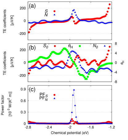
Figure 3: Chemical potential dependence of the thermoelectric quantities of $6\times 6$ SkX at $T=300$K: (a)$S$ and $N$, (b)$S_{0},\ N_{0}$(left axis) and $\theta_{H}$(right axis) [see Eq.(1)], (c)Power factors corresponding to $S$ and $N$. The blue dotted line for PF_N in (c) is drawn to guide the eye.

As to the longitudinal $S(\mu)$, it is largely affected by the anomalous effect when $\theta_{H}(\mu)$ is finite (almost throughout the plotted $\mu$ range)We recognize in Fig.3(a,b) the following three points (i)-(iii) including their explanation based on what we have seen in Fig.2: (i) $S({\mu_{0}})\simeq 0$ and $S_{0}({\mu_{0}})\simeq 0$, resulting from the combination of the above-mentioned behavior of $\sigma_{xx}|_{T=0}$ and $\sigma_{xy}|_{T=0}$, whose symmetrical centers came across with each other around $\mu_{0}$. (ii) Just below and above $\mu_{0}$, $S$ shows the peaks (the higher one reaching $\approx 80\mu$V/K) of the sign opposite to that of $S_{0}$ despite rather small Hall angle $\theta_{H}$ there. This is thanks to the large $N_{0}$ that satisfies $|\theta_{H}N_{0}|>|S_{0}|$. (iii) Between the central and edge energy range, $S$ is strongly suppressed compared to $S_{0}$ due to large $\theta_{H}$.

On the transverse part $N$, what we notice in Fig.3(a,b) and their interpretations are the following two points (i) and (ii): (i) Around $\mu_{0}$, it shows a large peak $N\simeq N_{0}\simeq 180\mu$V/K. This is because of $\theta_{H}(\mu_{0})\simeq 0$ [See Eq.(1)] and large $\sigma_{xy}^{\prime}(\mu_{0})$ (the prime indicating the derivative with respect to $\mu$ at $T=0$) as a result of the large anti-symmetry of $\sigma_{xy}$ around $\mu_{0}$, which affects $N_{0}$ approximately through the Mott’s relation [Eq.(2), later to be discussed quantitavely] $N_{0}\propto\sigma_{xy}^{\prime}/\sigma_{xx}$. (ii) Away from $\mu_{0}$, $N$ is strongly suppressed compared to $N_{0}$ due to large $\theta_{H}$, similarly to the relation between $S$ and $S_{0}$. This is different from the situation where $N_{0}$ is the far dominant contribution to $N$, as reported for example in Ref.[Hanasaki et al., 2008]. In view of the relation between $S$ and $N$, it is instructive that large $N$ appears thanks to the large asymmetry of $\sigma_{xy}$, at the same filling where $S$ diminishes due to the complete loss of asymmetry in $\sigma_{xx}$, showing that $\sigma_{xy}$ could be an additional freedom in seeking better thermoelectricity, when the material is properly designed.

V.3 Largest predicted thermoelectric voltages

In order to better capture quantitatively the above-mentioned connection between conductivities and TE coefficients that leads to large values of the latter, which are seemingly attractive for TE applications, let us check whether the largest value $S_{\rm max}$ and $N_{\rm max}$ seen in the central energy range in Fig.3(a) can be roughly estimated via the well-known Mott’s formula, which says,

$$\alpha_{ij}=-\frac{\pi^{2}}{3}\frac{k_{B}^{2}T}{e}\sigma_{ij}^{{}^{\prime}}(\mu)|_{T=0},$$ (2)

where the prime in $\sigma_{xy}^{\prime}$ means the derivative with regard to the Fermi energy (chemical potenatial $\mu$ at $T=0$). We write the chemical potential values that respectively give $S_{\rm max}$ and $N_{\rm max}$ as $\mu_{S}$ and $\mu_{N}$, both of which are close to $\mu_{0}$ but slightly different from each other. Finding that $S_{0}(\mu_{S})\approx 0,\ \theta_{H}(\mu_{S})\approx 1$, $S$ reduces to $S({\mu_{S}})\simeq N_{0}(\mu_{S})/2=\sigma_{xy}^{\prime}/{2\sigma_{xx}}$. Similarly found is that $N(\mu_{N})\simeq N_{0}(\mu_{N})$ because of $S_{0}(\mu_{N})\approx 0\approx\theta_{H}(\mu_{N})$. A rough estimation of $\sigma_{xy}^{\prime}(\mu_{S})|_{T=0}$ can be obtained by linearly-approximating the drastical drop of AHC $\Delta\sigma_{xy}(\mu)\approx-28(e^{2}/h)\Omega^{-1}$ in the energy range $\Delta\mu\approx 0.13$ eV in Fig.2(c). This gives $\sigma_{xy}^{\prime}(\mu_{S})\simeq\frac{\Delta\sigma_{xy}}{\Delta\mu}\approx 2.2\times 10^{2}(e^{2}/h)$eV^-1. The other quantity we need is $\sigma_{xx}(\mu_{S})$, which was found to be about $7.7(e^{2}/h)$. Combining these, a dimensionless factor of $x=k_{B}T/(\sigma_{xx}/\sigma_{xy}^{\prime})\simeq 0.73$ is found at $T=300{\rm K}\ (kT\simeq 0.026{\rm eV}$). Finally our evaluation arrives at $N_{\rm max}=N(\mu_{N})\simeq N(\mu_{S})\simeq N_{0}(\mu_{S})\simeq-\frac{\pi^{2}}{3}\frac{k_{B}}{e}x\approx 2\times 10^{2}\mu{\rm V/K}$ and therefore $S_{\rm max}=S(\mu_{S})\approx 1\times 10^{2}\mu{\rm V/K}$. These values are in fairly good accordance with the integration-derived values, hence clarifying that $T=300$K is low enough (in comparison to the Fermi level) for the Mott’s formula to be valid at least for rough estimation.

At this point we compare the maximum value of $\alpha_{xy}\approx 10^{-8}$ A/K corresponding to the above-estimated $N_{\rm max}$, with a value reasonably expected to be maximum within the low temperature approximation for the two-band Dirac-Zeeman (DZ) model we studied before Mizuta and Ishii (2015). The low-$T$ approximated $\alpha_{xy}$ in Eq.(4) of Ref.[Mizuta and Ishii, 2015] can be rewritten as a 2D quantity $\alpha_{xy}\simeq(\pi ke/12h)(kT/\Delta)/\tilde{\mu}^{2}$, where $\Delta$ is the Zeeman gap and $\tilde{\mu}\equiv\mu/\Delta\geq 1$ for the electron-doped case. Assuming rather small $\tilde{\mu}=2$, and choosing $(kT/\Delta)=0.3$ to loosely satisfy the low-$T$ criterion $kT\ll\mu-\Delta=\Delta$, we obtain $\alpha_{xy}\approx 10^{-10}$A/K for the DZ model, which is by two orders of magnitude smaller than in the $6\times 6$ SkX. Although some larger $\alpha_{xy}$ can be achieved beyond low-$T$ range, still larger values in the SkX should be ascribed to the AHC more than ten times larger than that of the DZ model.

Finally, since $N_{\rm max}\simeq 180\mu$V/K is a good enough value as a TE material, in order to further investigate the practical performance of the present system, we plot the powerfactor ${\rm PF}_{S}\equiv\sigma_{xx}S^{2}$ and ${\rm PF}_{N}\equiv\sigma_{xx}N^{2}$ in Fig.3(c). Note that, for the evaluation of power factors, unlike in the discussions of TE quantities up to now, we need to know $\sigma^{3D}_{xx}$. Therefore we assumed the SkX film thickness of 10nm. The maximum of ${\rm PF}_{N}\approx 10^{-3}$W/(K²m) is comparable to the values of possible oxide TE candidates such as NaCo₂O₄ and ZnO Gaultois et al. (2013). Although the thermal conductivity $\kappa$ was beyond the scope of this study, we just make a rough estimate here: Assuming the thermal conductivity $\kappa$ of the order of 1W/(Km) corresponding to good TE materials Gaultois et al. (2013), the present case realizes $Z_{N}T$ of the order of 0.3 at $T=300$K.

The main limitation of our results lies in the lack of knowledge on the processes through which electrons are scattered. Even if the single-$\tau$ approximation is valid, the magnitude of $\tau$ matters a lot. This is clearly manifested in the relation $N(\mu_{N})\propto\tau^{-1}$. For example we obtain $N(\mu_{N})\approx 20\mu$V/K if we suppose $\tau=1{\rm ps}$, although the Nernst coefficient of this size is still much larger than the so far reported values and is practically valuable Sakuraba (2016).

VI Summary

We computed the thermoelectric (TE) coefficients in a model of square skyrmion crystal, where spin-scalar-chirality-driven anomalous Hall/Nernst effects directly expressed in terms of Berry curvature in momentum space, were found to give rise to, not only a very different behavior in Seebeck coefficient from in the case of conventional TE materials, but also a surprisingly large Nernst coefficient. The future task is to understand the physics unique to such systems that leads to the prominent TE effect, and to find or design good TE materials among this class of materials using the first-principles method used here, which will also be of great practical importance for energy-saving applications.

Appendix A Expressions of conductivity tensors

We derive below the semiclassical formulae for conductivity tensors. The starting point is the expression for charge current ${\bf j}$ obtained in Ref.[Xiao et al., 2006], which reads,

$${\bf j} =e\int\frac{d{\bf k}}{(2\pi)^{2}}g({\bf r},{\bf k}){\bf v}_{\bf k}$$

$$+e\nabla_{\bf r}\times k_{\rm B}T({\bf r})\int\frac{d{\bf k}}{(2\pi)^{2}}{\bf\Omega}({\bf k})\log\left[1+\exp\left(-\frac{\varepsilon_{\bf k}-\mu}{k_{\rm B}T({\bf r})}\right)\right],$$ (3)

where $e,\ g({\bf r},{\bf k)},\ T({\bf r}),\ {\bf v}_{\bf k},\ \varepsilon_{\bf k},\ {\rm\Omega}({\bf k}),\ {\rm and}\ \mu$ stand for the electron’s charge ($e<0$), distribution function, local temperature, (velocity, energy and k-space Berry curvature) of an electron with wave number k and chemical potential, respectively.

The second term is a correction that appears when spatial inhomogeneity [$T({\bf r})$ in the present case] exists. Simplifying the second term following Ref.[Xiao et al., 2006] and substituting the set of equations of motion of a perturbed (by E field) Bloch electron

$${\bf v}_{\bf k}=\frac{1}{\hbar}\frac{\partial\varepsilon_{\bf k}}{\partial{\bf k}}-\dot{\bf k}\times{\bf\Omega}({\bf k}),\ \ \dot{\bf k}=e{\bf E}$$ (4)

which was derived in Ref.[Sundaram and Niu, 1999], for ${\bf v}_{\bf k}$ and the form of distribution

$$g({\bf r},{\bf k})=\tau_{\bf k}{\bf v}_{\bf k}\cdot\left[e{\bf E}+(\varepsilon_{\bf k}-\mu)\left(-\frac{\nabla T}{T}\right)\left(-\frac{\partial f}{\partial\varepsilon}\right)\right],$$ (5)

obtained as the solution of Boltzmann transport equation within relaxation time ($\tau_{\bf k}$) approximation, for $g({\bf r},{\bf k})$, we obtain

$$\left\{\begin{array}[]{l}{\displaystyle\sigma_{xx}=e^{2}\tau\int d{\bf k}\ v_{x}({\bf k})^{2}\left(-\frac{\partial f}{\partial\varepsilon}\right),\vspace{2mm}}\\ {\displaystyle\sigma_{xy}=-\frac{e^{2}}{\hbar}\int d{\bf k}\ \Omega_{z}({\bf k})=-\sigma_{yx},\vspace{2mm}}\\ {\displaystyle\alpha_{ij}=\frac{1}{e}\int d\varepsilon\sigma_{ij}(\varepsilon)|_{T=0}\frac{\varepsilon-\mu}{T}\left(-\frac{\partial f}{\partial\varepsilon}\right)}\\ \qquad\qquad{\rm for}\ \ \ \ i=x\ \ {\rm or}\ \ y,\ \ j=x\ \ {\rm or}\ \ y,\end{array}\right.$$ (6)

where $v_{x}({\bf k})\equiv\hbar^{-1}\partial\varepsilon({\bf k})/\partial k_{x}$ is the electron’s group velocity, and we assumed a constant relaxation time ($\tau_{\bf k}=\tau$).

Appendix B Comment on the topological Hall contribution

We roughly estimate the magnitude of change in our result to be brought about by considering $\sigma_{xy}^{T}$ omitted in the main part of the paper.

The expression for $\sigma_{xy}^{T}$ in the Drude model treatment is,

$$\sigma_{xy}^{T}=\frac{\omega_{s}\tau}{1+(\omega_{s}\tau)^{2}}\sigma_{xx},$$ (7)

where $\omega_{s}\equiv eB_{\rm spin}/m_{e}$ with spin-scalar-chirality-induced field $B_{\rm spin}\equiv(\hbar/2e)\hat{\bf m}\cdot(\partial_{x}\hat{\bf m}\times\partial_{y}\hat{\bf m})$ determined by the unit vector of the background spin texture $\hat{\bf m}\equiv{\bf m}/|{\bf m}|$ and electron mass $m_{e}$.

Substituting the present SkX form of $\hat{\bf m}({\bf r})$, we obtain the spatially-inhomogeneous $B_{\rm spin}({\bf r})=(\hbar/2e)(\pi/r\lambda)\sin\pi(1-r/\lambda)$, which gives a skyrmion size $\lambda$-independent flux of $h/e$ Hamamoto et al. (2015). Approximating by taking its unit-cell averaged value $\overline{B}_{\rm spin}=(h/e)/(\pi\lambda^{2})$ that is roughly $10^{3}$ T in our case of $\lambda\approx 1{\rm nm}$, we obtain the frequency of $\overline{\omega_{s}}=(e\overline{B}_{\rm spin}/m_{e}\approx 2\times 10^{14}{\rm s}^{-1}$ and thus $\overline{\omega_{s}}\tau\approx 20$ for the scattering-relaxation time of $\tau=0.1$ps assumed throughout this paper. Therefore, the contribution of $\sigma_{xy}^{T}\approx\sigma_{xx}/20$ adds less than 0.1 to $\theta_{H}$ and less than 0.1$S_{0}$ to $N_{0}$, which is good reason to omit $\sigma_{xy}^{T}$ in our case.

References

- Nagaosa et al. (2010) N. Nagaosa, J. Sinova, S. Onoda, A. H. MacDonald, and N. P. Ong, Rev. Mod. Phys. 82, 1539 (2010).
- Xiao et al. (2006) D. Xiao, Y. Yao, Z. Fang, and Q. Niu, Phys. Rev. Lett. 97, 026603 (2006).
- Xiao et al. (2010) D. Xiao, M. Chang, and Q. Niu, Rev. Mod. Phys. 82, 1959 (2010).
- Culcer et al. (2003) D. Culcer, A. MacDonald, and Q. Niu, Phys. Rev. B 68, 045327 (2003).
- Chang et al. (2013) C.-Z. Chang, J. Zhang, X. Feng, J. Shen, Z. Zhang, M. Guo, K. Li, Y. Ou, P. Wei, L.-L. Wang, Z.-Q. Ji, Y. Feng, S. Ji, X. Chen, J. Jia, X. Dai, Z. Fang, S.-C. Zhang, K. He, Y. Wang, L. Lu, X.-C. Ma, and Q.-K. Xue, Science 340, 167 (2013).
- Mizuta and Ishii (2014) Y. P. Mizuta and F. Ishii, JPS Conf. Proc. 3, 017035 (2014).
- Mizuta and Ishii (2015) Y. P. Mizuta and F. Ishii, JPS Conf. Proc. 5, 011023 (2015).
- Fang et al. (2014) C. Fang, M. J. Gilbert, and B. A. Bernevig, Phys. Rev. Lett. 112, 046801 (2014).
- Jiang et al. (2012) H. Jiang, Z. Qiao, H. Liu, and Q. Niu, Phys. Rev. B 85, 045445 (2012).
- Neubauer et al. (2009) A. Neubauer, C. Pfleiderer, B. Binz, A. Rosch, R. Ritz, P. G. Niklowitz, and P. Böni, Phys. Rev. Lett. 102, 186602 (2009).
- Yu et al. (2010) X. Yu, N. Kanazawa, Y. Onose, K. Kimoto, W. Zhang, S. Ishiwata, Y. Matsui, and Y. Tokura, Nature Mater. 10, 106 (2010).
- Skyrme (1962) T. Skyrme, Nucl. Phys. 31, 556 (1962).
- Mühlbauer et al. (2009) S. Mühlbauer, B. Binz, F. Jonietz, C. Pfleiderer, A. Rosch, A. Neubauer, R. Georgii, and P. Böni, Science 323, 915 (2009).
- Heinze et al. (2011) S. Heinze, K. von Bergmann, M. Menzel, J. Brede, A. Kubetzka, R. Wiesendanger, G. Bihlmayer, and S. Blügel, Nature Phys. 7, 713 (2011).
- Hamamoto et al. (2015) K. Hamamoto, M. Ezawa, and N. Nagaosa, Phys. Rev. B 92, 115417 (2015).
- Lado and Fernández-Rossier (2015) J. L. Lado and J. Fernández-Rossier, Phys. Rev. B 92, 115433 (2015).
- McCormick and Trivedi (2015) T. M. McCormick and N. Trivedi, Phys. Rev. A 91, 063609 (2015).
- Miyasato et al. (2007) T. Miyasato, N. Abe, T. Fujii, A. Asamitsu, S. Onoda, Y. Onose, N. Nagaosa, and Y. Tokura, Phys. Rev. Lett. 99, 086602 (2007).
- (19) T. Ozaki, H. Kino, J. Yu, M. J. Han, M. Ohfuti, F. Ishii, K. Sawada, Y. Kubota, T. Ohwaki, H. Weng, M. Toyoda, H. Kawai, Y. Okuno, R. Perez, P. P. Bell, T. Duy, Y. Xiao, A. M. Ito, and K. Terakura, Open source package for Material eXplorer, www.openmx-square.org .
- Mostofi et al. (2008) A. A. Mostofi, J. R. Yates, Y. S. Lee, I. Souza, D. Vanderbilt, and N. Marzari, Comput. Phys. Commun. 178, 685 (2008), www.wannier.org.
- Note (1) This value is expected to be realistic Shur et al. (1996), but we will find later in the discussions that our results are very sensitive to the choice of .
- Kurz et al. (2004) P. Kurz, F. Förster, L. Nordström, G. Bihlmayer, and S. Blügel, Phys. Rev. B 69, 024415 (2004).
- Kubler et al. (1972) J. Kubler, K. H. Hock, J. Sticht, and A. R. Williams, J. Phys. F. 18, 469 (1972).
- Wang et al. (2006) X. Wang, J. R. Yates, I. Souza, and D. Vanderbilt, Phys. Rev. B 74, 195118 (2006).
- Pizzi et al. (2014) G. Pizzi, D. Volja, B. Kozinsky, M. Fornari, and N. Marzari, Comput. Phys. Commun. 185, 422 (2014).
- Note (2) For the SkX, the calculated band structure and the Fermi energy dependence of AHC were in overall agreement with the ones reported in Ref.[\rev@citealpnumhamamotoquantized2015], confirming the reproducibility of the similar situation by different approaches, i.e., tight-binding model as in Ref.[\rev@citealpnumhamamotoquantized2015] and our first-principles treatment.
- Note (3) Our choice is just an example of suitable sets for finding large in the following sense: If we obtain larger bandwidths, e.g. by compressing the lattice (making smaller), while somehow keeping maximally the shape of Berry curvature, will be smaller, but thanks to the approximate relation [see Eq.(2)], at a higher temperature we may well get of the same magnitude as in the original system.
- Hanasaki et al. (2008) N. Hanasaki, K. Sano, Y. Onose, T. Ohtsuka, S. Iguchi, I. Kezsmarki, S. Miyasaka, S. Onoda, N. Nagaosa, and Y. Tokura, Phys. Rev. Lett. 100, 106601 (2008).
- Gaultois et al. (2013) M. W. Gaultois, T. D. Sparks, C. K. H. Borg, R. Seshadri, W. D. Bonificio, and D. R. Clarke, Chem. Mater. 25, 2911 (2013).
- Sakuraba (2016) Y. Sakuraba, Scr. Mater. 111, 29 (2016).
- Sundaram and Niu (1999) G. Sundaram and Q. Niu, Phys. Rev. B 59, 14915 (1999).
- Shur et al. (1996) M. Shur, B. Gelmont, and M. Asif Khan, J. Electron. Mater. 25, 777 (1996).