Analytic derivation of the next-to-leading order proton structure function $F_{2}^{p}(x,Q^{2})$ based on the Laplace transformation

Abstract

An analytical solution based on the Laplace transformation technique for the Dokshitzer-Gribov-Lipatov-Altarelli-Parisi DGLAP evolution equations is presented at next-to-leading order accuracy in perturbative QCD. This technique is also applied to extract the analytical solution for the proton structure function, $F_{2}^{p}(x,Q^{2})$, in the Laplace $s$-space. We present the results for the separate parton distributions for all parton species, including valence quark densities, the anti-quark and strange sea parton distribution functions (PDFs), and the gluon distribution. We successfully compare the obtained parton distribution functions and the proton structure function with the results from GJR08 [Eur. Phys. J C 53 (2008) 355-366] and KKT12 [J. Phys. G 40 (2013) 045002] parametrization models as well as the $x$-space results using QCDnum code. Our calculations show a very good agreement with the available theoretical models as well as the deep inelastic scattering (DIS) experimental data throughout the small and large values of $x$. The use of our analytical solution to extract the parton densities and the proton structure function is discussed in detail to justify the analysis method considering the accuracy and speed of calculations. Overall, the accuracy we obtain from the analytical solution using the inverse Laplace transform technique is found to be better than 1 part in 10⁴ to 10⁵. We also present a detailed QCD analysis of non-singlet structure functions using all available DIS data to perform global QCD fits. In this regard we employ the Jacobi polynomial approach to convert the results from Laplace $s$ space to Bjorken $x$ space. The extracted valence quark densities are also presented and compared to the JR14, MMHT14, NNPDF and CJ15 PDFs sets. We evaluate the numerical effects of target mass corrections (TMCs) and higher twist (HT) terms on various structure functions, and compare fits to data with and without these corrections.

I Introduction

Dokshitzer-Gribov-Lipatov-Altarelli-Parisi (DGLAP) evolution equations Dokshitzer:1977sg ; Gribov:1972ri ; Lipatov:1974qm ; Altarelli:1977zs are a set of an integro differential equations which can be used to evolve the parton distribution functions (PDFs) to an arbitrary energy scale, Q². The solutions of the DGLAP evolution equations will provide us the gluon, valence quark and sea quark distributions inside the nucleon. Consequently these equations can be used widely as fundamental tools to extract the deep inelastic scattering (DIS) structure functions (SFs) of the proton, neutron, and deuteron to enrich our current information about the structure of hadrons. The standard procedure to obtain the $x$ dependence of the gluon and quark distributions is to solve numerically the DGLAP equations and compare the solutions with the data in order to fit the PDFs to some initial factorization scale, typically less than the square of the $c$-quark mass Q${}_{0}^{2}\approx$ ($m_{c}^{2}\approx$2 GeV²). The initial distributions for the gluon and quark are usually determined in a global QCD analysis including a wide variety of DIS data from HERA Abramowicz:2016ztw ; Abt:2016zth ; Abramowicz:2015mha ; Aaron:2009kv ; Aaron:2009bp ; Aaron:2009aa and COMPASS Adolph:2015saz , hadron collisions at Tevatron Aaltonen:2008eq ; Abazov:2008ae ; Abulencia:2007ez ; Abbott:2000ew fixed-target experiments over a large range of $x$ and Q², as well as $\nu(\bar{\nu}){\rm N}\ xF_{3}$ data from CHORUS and NuTeV Onengut:2005kv ; Tzanov:2005kr , and also the data for the longitudinal structure function $F_{\rm L}(x,Q^{2})$ Collaboration:2010ry . Finally using the coupled integro-differential DGLAP evolution equations one can find the PDFs at higher energy scale, Q². For the most recent studies on global QCD analysis, see for instance Harland-Lang:2014zoa ; Khanpour:2012tk ; Alekhin:2012ig ; ::2014uva ; Buckley:2014ana ; Ball:2014uwa ; Martin:2009iq ; JimenezDelgado:2008hf .

Some analytical solutions of the DGLAP evolution equations using the Laplace transform technique, initiated by Block et al., have been reported in recent years Block:2010du ; Block:2011xb ; Block:2010fk ; Block:2009en ; Block:2010ti ; Block:2007pg ; Block:2008xc ; Zarei:2015jvh ; AtashbarTehrani:2013qea ; Boroun:2015cta ; Boroun:2014dka with considerable phenomenological success. In this paper, a detailed analysis has been performed, using repeated Laplace transforms, in order to find an analytical solutions of the DGLAP evolution equations at next-to-leading order (NLO) approximations. We also analytically calculate the individual gluon, singlet and non-singlet quark distributions from the initial distributions inside the nucleon. We present our results for the valence quark distributions $xu_{v}$ and $xd_{v}$, the anti quark distributions $x(\overline{d}+\overline{u})$ and $x\Delta=x(\overline{d}-\overline{u})$, the strange sea distribution $xs=x\overline{s}$, and finally the gluon distribution $xg$. Using the Laplace transform technique, we also extract the analytical solutions for the proton structure function $F_{2}^{p}(x,Q^{2})$ as the sum of flavor singlet $F_{2}^{\rm S}(x,Q^{2})$, $F_{2}^{\rm g}(x,Q^{2})$ and flavor non singlet $F_{2}^{\rm NS}(x,Q^{2})$ distributions. The obtained results indicate an excellent agreement with the DIS data as well as those obtained by other methods such as the fit to the $F_{2}^{p}$ structure function performed by KKT12 Khanpour:2012tk and GJR08 Gluck:2007ck .

In the present work, we also demonstrate once more the compatibility of the Laplace transform technique and the Jacobi polynomial expansion approach at the next-to-leading order and extract the valence quark densities as well as the values of the parameter $\alpha_{s}(M_{Z}^{2})$ from the QCD fit to the recent DIS data. The effect of target mass corrections (TMCs), which are important especially in the high-$x$ and low-Q² regions, and the contribution from higher twist (HT) terms are also considered in the analysis. To quantify the size of these corrections, we evaluate the structure functions at next-to-leading order in QCD, and compare the results with the DIS data used in our PDF fits.

The present paper is organized as follows: In Sec. II, we provide a brief discussion of the theoretical formalism of the proton structure function $F_{2}^{p}(x,Q^{2})$ at the NLO approximation of QCD. A detailed formalism to establish an analysis method for the solution of DGLAP evolution using the repeated Laplace transforms for the singlet sector have been presented in Sec. III. In Sec. IV, we also review the method of the analytical solution of DGLAP evolution equations based on Laplace transformation techniques for the non singlet sector. In Sec. V, we utilize this method to calculate the proton structure function $F_{2}^{p}(x,Q^{2})$ by Laplace transformation. We attempt a detailed comparison of our next-to-leading order results with recent results from the literature in Sec. VI. We also discuss in detail the use of our analytical solution to justify the analysis method in terms of accuracy and speed. A completed comparison between the obtained results and available DIS data is also presented in this section. The application of the Laplace transformation techniques and Jacobi polynomial expansion machinery at the next-to-leading order are described in detail in Sec. VII. The method of the QCD analysis including the PDF parametrization, statistical procedures, and data selection are also presented in this section. The numerical effects of target mass corrections (TMCs) and higher twist terms (HT) on various structure functions are also discussed. Finally, we give our summary and conclusions in Sec. VIII. In Appendix A, we render the results for the different splitting functions in the Laplace transformed $s$ space, and Appendix B includes the analytical expression for the coefficient functions of the singlet and gluon distribution in $s$ space.

II Theoretical formalism

The present DIS and hadron collider data provide the best determination of quark and gluon distributions in a wide range of $x$ Abramowicz:2015mha ; Aaron:2009bp ; Aaron:2009aa . In this article we will be concerned specifically with the proton structure function at next-to-leading order accuracy in perturbative QCD. In the common $\overline{\rm MS}$ renormalization scheme the $F_{2}(x,Q^{2})$ structure function, extracted from the DIS $ep$ process, can be written as the sum of a flavour singlet $F_{2,{\rm S}}(x,Q^{2})$, $F_{2,g}(x,Q^{2})$ and a flavour non-singlet $F_{2,{\rm NS}}(x,Q^{2})$ distributions in which we will have,

$$\frac{F_{2}(x,Q^{2})}{x} = \frac{1}{x}\left(F_{2,{\rm S}}(x,Q^{2})+F_{2,g}(x,Q^{2})+F_{2,{\rm NS}}(x,Q^{2})\right)$$ (1)

$$= <e^{2}>C_{2,{\rm S}}(x,Q^{2})\ \otimes\ q_{\rm S}(x,Q^{2})$$

$$+ <e^{2}>C_{2,{\rm g}}(x,Q^{2})\ \otimes\ g(x,Q^{2})$$

$$+ C_{2,{\rm NS}}(x,Q^{2})\ \otimes\ q_{\rm NS}(x,Q^{2})\,,$$

here $g$ and $q_{i}$ represent the gluon and quark distribution functions respectively. The $q_{\rm NS}$ stands for the usual flavour non-singlet combination, $xu_{v}=x(u-\bar{u})$, $xd_{v}=x(d-\bar{d})$ and $q_{\rm S}$ stand for the flavour-singlet quark distribution,

$$xq_{\rm S}=\sum_{i=1}^{N_{f}}x(q_{i}+\bar{q}_{i})\,,$$

where $N_{f}$ denotes the number of active massless quark flavours. In Equation (1) the $\otimes$ symbol denotes the convolution integral which turns into a simple multiplication in Mellin $N$ space and $<e^{2}>$ represents the average squared charge. $C_{2,{\rm S}}$ and $C_{2,{\rm NS}}$ are the common next-to-leading order Wilson coefficient functions Vermaseren:2005qc . The analytical expression for the additional next-to-leading order gluonic coefficient function $C_{2,{\rm g}}$ can be found in Ref. Vermaseren:2005qc . As we already mentioned the gluon and quark distribution functions at the initial state $Q_{0}^{2}$ can be determined by fit to the precise experimental data over a large numerical range for $x$ and Q². The individual quark and gluon distributions are parametrized with the pre-determined shapes as a standard functional form. This function is given in terms of $x$ and a chosen value for the input scale Q${}_{0}^{2}$. The gluon distribution $xg(x,Q_{0}^{2})$ is a far more difficult case for PDF parametrizations to obtain precise information due to the small constraints provided by the recent data Khanpour:2012tk ; Martin:2009iq .

In the following, we will present our analytic method based on the newly developed Laplace transform technique to determine the non singlet $F_{\rm NS}(x,Q^{2})$ and singlet $F_{\rm S}(x,Q^{2})$ and $G(x,Q^{2})$ structure functions using the input distributions $F_{\rm NS0}(x,Q_{0}^{2})$, $F_{\rm S0}(x,Q_{0}^{2})$ and $G_{0}(x,Q_{0}^{2})$ at Q${}_{0}^{2}$ = 2 GeV². We use the KKT12 Khanpour:2012tk and GJR08 Gluck:2007ck input parton distributions to determine the individual parton distribution functions at an arbitrary Q² > Q${}_{0}^{2}$, which can be obtained, using the DGLAP evolution equations. Having the parton distribution functions and using the inverse Laplace transform, one can extract the proton structure function $F_{2}^{p}(x,Q^{2})$ as a function of $x$ at any desired Q² value.

III Singlet solution in Laplace space at the next-to-leading order approximation

For the most important high energy processes the next-to-leading order approximation is the standard one which we also consider it in our analysis. The DGLAP evolution equations can describe the perturbative evolution of the singlet $xq_{\rm S}(x,Q^{2})$ and gluon $xg(x,Q^{2})$ distribution functions. The coupled DGLAP evolution equations at the next-to-leading order approximation, using the convolution symbol $\otimes$, can be written as  Block:2007pg ; Block:2008xc

$$\frac{4\pi}{\alpha_{s}(Q^{2})}\frac{\partial F_{\rm S}}{\partial lnQ^{2}}(x,Q^{2})=F_{\rm S}\otimes\left(P_{qq}^{0}+\frac{\alpha_{s}(Q^{2})}{4\pi}P_{qq}^{1}\right)(x,Q^{2})$$

$$+\ G\otimes\left(P_{qg}^{0}+\frac{\alpha_{s}(Q^{2})}{4\pi}P_{qg}^{1}\right)(x,Q^{2})\,,$$ (2)

$$\frac{4\pi}{\alpha_{s}(Q^{2})}\frac{\partial G}{\partial lnQ^{2}}(x,Q^{2})=F_{\rm S}\otimes\left(P_{gq}^{0}+\frac{\alpha_{s}(Q^{2})}{4\pi}P_{gq}^{1}\right)(x,Q^{2})$$

$$+\ G\otimes\left(P_{gg}^{0}+\frac{\alpha_{s}(Q^{2})}{4\pi}P_{gg}^{1}\right)(x,Q^{2})\,,$$ (3)

where $\alpha_{s}(Q^{2})$ is the running coupling constant and the splitting functions $P_{ij}^{0}(x,\alpha_{s}(Q^{2}))$ and $P_{ij}^{1}(x,\alpha_{s}(Q^{2}))$ are the Altarelli-Parisi splitting kernels at one and two loop corrections respectively as Altarelli:1977zs ; Curci:1980uw ; Furmanski:1980cm ,

$$P_{ij}(x,\alpha_{s}(Q^{2}))=P_{ij}^{\rm LO}(x)+\frac{\alpha_{s}(Q^{2})}{2\pi}P_{ij}^{\rm NLO}(x)\,.$$ (4)

In the evolution equations, we take N_f = 4 for $m^{2}_{c}<\mu^{2}<m^{2}_{b}$ and N_f = 5 for $m^{2}_{b}<\mu^{2}<m^{2}_{t}$ and adjust the QCD parameter $\Lambda$ at each heavy quark mass threshold, $\mu^{2}=m^{2}_{c}$ and $m^{2}_{b}$. Consequently the renormalized coupling constant $\alpha_{s}(Q^{2})$ can be run continuously when the N_f changes at the $c$ and $b$ mass thresholds Botje:2010ay .

We are now in a position to briefly review the method of extracting the parton distribution functions via analytical solution of DGLAP evolution equation using the Laplace transformation technique. By considering the variable changes $\nu\equiv\ln(1/x)$ and $w\equiv\ln(1/z)$, one can rewrite the evolution equations presented in Eqs.(III) and (III) in terms of the convolution integrals and with respect to $v$ and $\tau$ variables as Block:2010du ; Zarei:2015jvh

$$\frac{\partial{\hat{F}}_{\rm S}}{\partial\tau}(\nu,\tau)=$$

$$\int_{0}^{\nu}\left({\hat{K}}_{qq}(\nu-w)\ +\ \frac{\alpha_{s}(\tau)}{4\pi}{\hat{K}}_{qq}^{1}(\nu-w)\right){\hat{F}}_{\rm S}(w,\tau)d\,w$$

$$+\int_{0}^{\nu}\left({\hat{K}}_{qg}(\nu-w)\ +\ \frac{\alpha_{s}(\tau)}{4\pi}{\hat{K}}_{qg}^{1}(\nu-w)\right){\hat{G}}(w,\tau)d\,w$$

$$\frac{\partial{\hat{G}}}{\partial\tau}(\nu,\tau)=$$

$$\int_{0}^{\nu}\left({\hat{K}}_{gq}(\nu-w)\ +\ \frac{\alpha_{s}(\tau)}{4\pi}{\hat{K}}_{gq}^{1}(\nu-w)\right){\hat{F}}_{\rm S}(w,\tau)d\,w$$

$$+\int_{0}^{\nu}\left({\hat{K}}_{gg}(\nu-w)\ +\ \frac{\alpha_{s}(\tau)}{4\pi}{\hat{K}}_{gg}^{1}(\nu-w)\right){\hat{G}}(w,\tau)d\,w,$$

where the Q² dependence of above evolution equations is expressed entirely thorough the variable $\tau$ as $\tau(Q^{2},Q_{0}^{2})\equiv{1\over 4\pi}\int_{Q^{2}_{0}}^{Q^{2}}\alpha_{s}({Q^{\prime}}^{2})d\ \ln{Q^{\prime}}^{2}$. Note that we used the notation $\hat{F}_{\rm S}(\nu,\tau)\equiv F_{\rm S}(e^{-\nu},Q^{2})$ and $\hat{G}(\nu,\tau)\equiv G(e^{-\nu},Q^{2})$. The above convolution integrals show that using one-loop ${\hat{K}}_{ij}^{0}(\nu)\equiv e^{-\nu}P_{ij}^{0}(e^{-\nu})$ and two-loop ${\hat{K}}_{ij}^{1}(\nu)\equiv e^{-\nu}P_{ij}^{1}(e^{-\nu})$ kernels where the $i$ and $j$ are a combination of quark $q$ or gluon $g$, one can obtain the singlet ${\hat{F}}_{\rm S}(\nu,\tau)$ and gluon ${\hat{G}}(\nu,\tau)$ sectors of distributions.

Defining the Laplace transforms $f(s,\tau)\equiv{\cal L}[\hat{F}_{\rm S}(\nu,\tau);s]$ and $g(s,\tau)\equiv{\cal L}[\hat{G}(\nu,\tau);s]$ and using this fact that the Laplace transform of a convolution factors is simply the ordinary product of the Laplace transform of the factors, which have been presented in  Block:2010du ; Block:2011xb , the Laplace transforms of Eqs.(III), and (III) convert to ordinary first-order differential equations in Laplace space $s$ with respect to variable $\tau$. Therefore we will arrive at

$${\partial f\over\partial\tau}(s,\tau) = \left(\Phi_{f}^{\rm LO}(s)\ +\ \frac{\alpha_{s}(\tau)}{4\pi}\Phi_{f}^{\rm NLO}(s)\right)f(s,\tau)$$ (7)

$$+ \left(\Theta_{f}^{\rm LO}(s)\ +\ \frac{\alpha_{s}(\tau)}{4\pi}\Theta_{f}^{\rm NLO}(s)\right)g(s,\tau)\,,$$

$${\partial g\over\partial\tau}(s,\tau) = \left(\Phi_{g}^{\rm LO}(s)\ +\ \frac{\alpha_{s}(\tau)}{4\pi}\Phi_{g}^{\rm NLO}(s)\right)g(s,\tau)$$ (8)

$$+ \left(\Theta_{g}^{\rm LO}(s)\ +\ \frac{\alpha_{s}(\tau)}{4\pi}\Theta_{g}^{\rm NLO}(s)\right)f(s,\tau)\,,$$

whose the leading-order splitting functions for the structure function $F_{2}$, presented in Altarelli:1977zs ; Floratos:1981hs in Mellin space, are given by $\Phi_{(f,g)}^{\rm{LO}}$ and $\Theta_{(f,g)}^{\rm{LO}}$ at Laplace $s$ space by

$$\Phi_{f}^{\rm{LO}}=4-\frac{8}{3}\left(\frac{1}{s+1}+\frac{1}{s+2}+2\left(\gamma_{E}+\psi(s+1)\right)\right)\,,$$ (9)

$$\Theta_{f}^{\rm{LO}}=2N_{f}\left(\frac{1}{1+s}-\frac{2}{2+s}+\frac{2}{3+s}\right)\,,$$ (10)

$$\Phi_{g}^{\rm{LO}} = 12\left(\frac{1}{s}-\frac{2}{1+s}+\frac{1}{2+s}-\frac{1}{3+s}-\left(\gamma_{E}+\psi(s+1)\right)\right)$$ (11)

$$+\frac{33-2N_{f}}{3}\,,$$

and

$$\Theta_{g}^{\rm{LO}}=\frac{8}{3}\left(\frac{2}{s}-\frac{2}{1+s}+\frac{1}{2+s}\right)\,,$$ (12)

where the N_f is the number of active quark flavors, $\gamma_{E}$ is the Euler’s constant and $\psi$ is the digamma function. The next-to-leading order splitting functions $\Phi_{(f,g)}^{\rm NLO}$ and $\Theta_{(f,g)}^{\rm NLO}$ are too lengthy to be include here and we present them in Appendix A. One can easily determine these next-to-leading order splitting functions in Laplace $s$ space using the next-to-leading order results derived in Ref. Altarelli:1977zs ; Curci:1980uw ; Furmanski:1980cm . The leading-order solution of the coupled ordinary first order differential equations in Eqs.(7) and (8) in terms of the initial distributions are straightforward. Considering the initial distributions for the gluon, $g^{0}(s)$, and singlet distributions, $f^{0}(s)$, at the input scale Q${}_{0}^{2}=2$ GeV², the evolved solutions in the Laplace $s$ space are given by Block:2010du ; Block:2011xb ,

$$f(s,\tau) = k_{ff}(s,\tau)f^{0}(s)\ +\ k_{fg}(s,\tau)g^{0}(s)$$

$$g(s,\tau) = k_{gg}(s,\tau)g^{0}(s)\ +\ k_{gf}(s,\tau)f^{0}(s),$$ (13)

The inverse Laplace transform of coefficients $k$ in the above equations are defined as kernels $K_{ij}(\nu,\tau)\equiv{\cal L}^{-1}[k_{ij}(s,\tau);\nu]$ and the input distributions by $\hat{F}_{\rm S}^{0}(\nu)\equiv{\cal L}^{-1}[f^{0}(s);\nu]$ and $\hat{G}^{0}(\nu)\equiv{\cal L}^{-1}[g^{0}(s);\nu]$. Then the following decoupled solutions with respect to $\nu$ and Q² variables and in terms of the convolutions integrals can be written as,

$$\hat{F}_{\rm S}(\nu,Q^{2})=\int_{0}^{v} K_{\rm FF}(\nu-w,\tau)\hat{F}_{\rm S}^{0}(w)\,dw$$

$$+ \int_{0}^{\nu}K_{\rm FG}(\nu-w,\tau)\hat{G}_{0}(w)\,dw,$$ (14)

$$\hat{G}(\nu,Q^{2})=\int_{0}^{\nu} K_{\rm GG}(\nu-w,\tau)\hat{G}_{0}(w)\,dw$$

$$+ \int_{0}^{\nu}K_{\rm GF}(\nu-w,\tau)\hat{F}_{\rm S}^{0}(w)\,dw.$$ (15)

Considering the $\nu\equiv ln(1/x)$, one can finally arrive at the solutions of the DGLAP evolution equations with respect to $x$ and Q² variables. As we mentioned earlier, the $Q^{2}$ dependence of the distributions functions $\hat{F}_{\rm S}(\nu,Q^{2})$ and $\hat{G}(v,Q^{2})$ are specified by $\tau$ variable. Clearly knowledge of the initial distributions $F_{\rm S}^{0}(x)$ and $G^{0}(x)$ at $Q_{0}^{2}$ is needed to obtained the distributions at any arbitrary energy scale $Q^{2}$

Now we intend to extend our calculations to the next-to-leading order approximation for gluon and singlet sectors of unpolarized parton distributions. In this case, to decouple and to solve DGLAP evolutions in Eqs.(7) and (8) we need an extra Laplace transformation from $\tau$ space to $U$ space. The $U$ will be a parameter in this new space. In the rest of the calculation, the $\alpha_{s}(\tau)/4\pi$ is replaced for brevity by $a(\tau)$. Therefore the solution of the first-order differential equations in Eqs.(7) and (8) can be converted to

$$U {\cal F}(s,U)-f^{0}(s)=\Phi_{f}^{\rm LO}(s){\cal F}(s,U)$$

$$+\Phi_{f}^{\rm NLO}(s)\ {\cal L}[a(\tau)f(s,\tau);U]$$

$$+\Theta_{f}^{\rm LO}(s){\cal G}(s,U)+\Theta_{f}^{\rm NLO}(s)\ {\cal L}[a(\tau)g(s,\tau);U]\,,$$

$$U {\cal G}(s,U)-g^{0}(s)=\Phi_{g}^{\rm LO}(s){\cal G}(s,U)$$

$$+\Phi_{g}^{\rm NLO}(s)\ {\cal L}[a(\tau)g(s,\tau);U]$$

$$+\Theta_{g}^{LO}(s){\cal F}(s,U)+\Theta_{g}^{\rm NLO}(s)\ {\cal L}[a(\tau)f(s,\tau);U]\,.$$

We can consider a very simple parametrization for $a(\tau)$ as $a(\tau)=a_{0}$ . Generally to do a more precise calculation at the next-to-leading order approximation, one can consider the following expression for the $a(\tau)$ as Zarei:2015jvh

$$a(\tau)\approx a_{0}+a_{1}e^{-b_{1}\tau}\,.$$ (18)

This expansion involves excellent accuracy to a few parts in $10^{4}$. Using $a(\tau)$ defined in the above equation and the conventions which were presented in Block:2010du ; Block:2011xb , the following simplified notations for the splitting functions in $s$ space can be introduced by:

$$\Phi_{f,g}(s)\equiv\Phi_{f,g}^{\rm LO}(s)+a_{0}\Phi_{f}^{\rm NLO}(s),$$

$$\Theta_{f,g}(s)\equiv\Theta_{g}^{\rm LO}(s)+a_{0}\Theta_{g}^{\rm NLO}(s)\;.$$ (19)

Equations.(III) and (III) can be solved simultaneously to get the desired coupled algebraic equations for singlet ${\cal F}(s,U)$ and gluon ${\cal G}(s,U)$ distributions arriving at,

$$\left[U-\Phi_{f}(s)\right]{\cal F}(s,U)-\Theta_{f}(s){\cal G}(s,U)=$$

$$f^{0}(s) +a_{1}\left[\Phi_{f}^{\rm NLO}(s){\cal F}(s,U+b_{1})+\Theta_{f}^{\rm NLO}(s){\cal G}(s,U+b_{1})\right]\,,$$

$$-\Theta_{g}(s){\cal F}(s,U)+\left[U-\Phi_{g}(s)\right]{\cal G}(s,U)=$$

$$g^{0}(s) +a_{1}\left[\Theta_{g}^{\rm NLO}(s){\cal F}(s,U+b_{1})+\Phi_{g}^{\rm NLO}(s){\cal G}(s,U+b_{1})\right]\,.$$

The simplified solutions of above equations can be obtained by setting $a_{1}=0$ in Eq.(18). For $a(\tau)=a_{0}$, the Eqs.(III) and (III) lead us to,

$$\left[U-\Phi_{f}(s)\right]{\cal F}_{1}(s,U)-\Theta_{f}(s){\cal G}_{1}(s,U)=f^{0}(s)\,,$$ (22)

$$-\Theta_{g}(s){\cal F}_{1}(s,U)+\left[U-\Phi_{g}(s)\right]{\cal G}_{1}(s,U)=g^{0}(s)\,.$$ (23)

One can easily solve these equations and extract the ${\cal F}_{1}(s,U)$ and ${\cal G}_{1}(s,U)$ distributions. The results are clearly based on the input quarks $f^{0}(s)$ and $g^{0}(s)$ gluon distribution functions at Q${}_{0}^{2}$. Using the Laplace transform technique, it is possible to go back from $U$ space to $\tau$ space, leading to the desired $f(s,\tau)$ and $g(s,\tau)$ expressions. The complete solutions of Eqs. (III) and (III) can be obtained via iteration processes. The iteration can be continued to any required order but we will restrict ourselves to getting a sufficient convergence of the solutions. Our results show that the second order of iterations is sufficient to get a reasonable convergence. Using the iterative solution of Eqs. (III) and (III) and the inverse Laplace transform technique to get back from $U$ space to $\tau$ space, the following expressions for the singlet and gluon distributions can be obtained Block:2010du ; Block:2011xb ; AtashbarTehrani:2013qea :

$$f(s,\tau) = k_{ff}(a_{1},b_{1},s,\tau)\,f^{0}(s)+k_{fg}(a_{1},b_{1},s,\tau)\,g^{0}(s)\,,$$

$$g(s,\tau) = k_{gg}(a_{1},b_{1},s,\tau)\,g^{0}(s)+k_{gf}(a_{1},b_{1},s,\tau)\,f^{0}(s)\,,$$

The analytical expressions for the next-to-leading order approximation of coefficients $k_{ff}$, $k_{fg}$, $k_{gf}$ and $k_{gg}$ up to the desired steps of iteration are given in Appendix B. Using Laplace inversion in Eq. (III) from $s$ to $\nu$ space, we can arrive to the decoupled solutions ($\nu$, $\tau$) space as the result of convolution defined by the Eqs. (III) and (15).

As a brief description, we have used the Laplace transform algorithm presented in Refs. Block:2009en ; Block:2010ti for the numerical inversion of Laplace transformations and convolutions to obtain the required parton distribution functions. The analytical result at the LO approximation is given by Eq. (III). Employing the iterative numerical method through Eq. (III) -(23), up to desired order to achieve a sufficient convergence, will yield us the analytical expressions for the patron densities in $s$ space at the NLO approximation given by Eq. (III). To return the distributions to the $\nu$ space we need to convolution integral, Eqs. (III) and (15) in both LO and the NLO approximations. The Q² dependence of the solutions are determined by the $\tau$ variable and recalling that $\nu\equiv\ln(1/x)$, the solutions can be transformed back into the usual $x$ space. Consequently, one can obtain the singlet and gluon distributions as $F_{S}(x,Q^{2})$ and $G(x,Q^{2})$ respectively.

We have used the numerical Laplace transform algorithm presented in Refs. Block:2009en ; Block:2010ti for the numerical inversion of Laplace transformations and convolutions to obtain the parton distribution functions and structure function in $x$ and $Q^{2}$ space.

IV Non-singlet solution in Laplace space at the next-to-leading order approximation

Here we wish to extend our calculations to the next-to-leading order approximation for the non singlet sector of the parton distributions. For the non singlet distribution $F_{\rm NS}(x,Q^{2})$, one can schematically write the logarithmic derivative of $F_{\rm NS}$ as a convolution of non-singlet distribution $F_{\rm NS}(x,Q^{2})$ with the non-singlet splitting functions, $p_{qq}^{\rm LO,NS}$ and $p_{qq}^{\rm NLO,NS}$ Altarelli:1977zs ; Curci:1980uw ; Furmanski:1980cm . Therefore the next-to-leading order contributions for the $F_{\rm NS}(x,Q^{2})$ can be written as:

$$\frac{4\pi}{\alpha_{s}(Q^{2})} \frac{\partial F_{\rm NS}}{\partial lnQ^{2}}(x,Q^{2})$$

$$=F_{NS}\otimes\left(p_{qq}^{\rm LO,NS}+\frac{\alpha_{s}(Q^{2})}{4\pi}p_{qq}^{\rm NLO,NS}\right)(x,Q^{2})\,.$$

Again changing to the required variable, $\nu\equiv\ln(1/x)$, and going to the Laplace space $s$, we arrive at the simple solution as,

$$\frac{\partial\hat{F}_{\rm NS}}{\partial\tau}(\nu,\tau) =\int_{0}^{\nu}\left(p_{qq}^{\rm LO,NS}(\nu-w)\right.+$$

$$\left.\frac{\alpha_{s}(\tau)}{4\pi}p_{qq}^{\rm NLO,NS}(\nu-w)\right)\hat{F}_{\rm NS}(w,\tau)e^{-(\nu-w)}\,dw\,.$$

Going to Laplace $s$ space, we can obtain the first-order differential equations in Laplace space $s$ with respect to the $\tau$ variable for the non-singlet distributions $f_{\rm NS}(s,\tau)$:

$$\frac{\partial f_{\rm NS}}{\partial\tau}(s,\tau)=\left(\Phi_{\rm NS}^{\rm LO}+\frac{\alpha_{s}(\tau)}{4\pi}\Phi_{\rm NS,qq}^{\rm NLO}\right)f_{\rm NS}(s,\tau)\,.$$ (27)

The above equation has a very simplified solution,

$$f_{\rm NS}(s,\tau)=e^{\tau\Phi_{\rm NS}(s)}f^{0}_{\rm NS}(s)\,,$$ (28)

where $\Phi_{\rm NS}(s)$ is contains the next-to-leading order contributions of the splitting functions at $s$ space, defined as

$$\Phi_{\rm NS}(s)\equiv\Phi_{\rm NS}^{\rm LO}(s)+\frac{\tau_{2}}{\tau}\Phi_{\rm NS,qq}^{\rm NLO}(s)\,.$$ (29)

The evaluation of $\Phi_{\rm NS,qq}^{\rm NLO}(s)={\cal L}\left[e^{-\nu}p_{qq}^{\rm NLO,NS}(e^{-\nu});s\right]$ is straightforward but too lengthy to present here. The analytical results for the unpolarized splitting functions in the transformed Laplace $s$ space at the next-to-leading order approximation are given in Appendix A. The Q² dependence of the evolution equations is represented by $\tau$ at the leading order approximation and by $\tau_{2}$ at the next-to-leading order approximation which the latter one defined as Block:2010du ; Block:2011xb ; AtashbarTehrani:2013qea ,

$$\tau_{2}\equiv\frac{1}{4\pi}\int_{0}^{\tau}\alpha(\tau^{\prime})d\tau^{\prime}\ =\ (\frac{1}{4\pi})^{2}\int_{Q_{0}^{2}}^{Q^{2}}\alpha_{s}^{2}(Q^{\prime 2})\ d\ln Q^{\prime 2}\,.$$

Since all parts of the current analysis are done at the next-to-leading order approximation, we should use the $\tau_{2}$ variable as well. However to simplify in notation, the $\tau$ variable is used insteadly through out the whole paper.

Similar to the singlet case, any non-singlet solution, $F_{\rm NS}(x,Q^{2})$, can be obtained using the non-singlet kernel $K_{\rm NS}\equiv{\cal L}^{-1}[e^{\tau\Phi_{\rm NS}(s)};\nu]$ which is defined by,

$$\hat{F}_{\rm NS}(\nu,\tau)=\int_{0}^{\tau}K_{\rm NS}(\nu-w)\hat{F}_{\rm NS}^{0}(w)dw\,.$$ (31)

Using again the appropriate change of variable, $\nu\equiv ln(1/x)$, the solution of Eq.(31) can be converted to the usual $(x,Q^{2})$ space. The iterative numerical method of Laplace transformations at the NLO approximation is followed by the convolutions, based on Eqs. (III) and (15). For the numerical inversion of Laplace transformations and convolutions to obtain the appropriate PDFs and SF in $x$ and $Q^{2}$ space, we again used the numerical inversion routine presented in Refs. Block:2009en ; Block:2010ti .

V Proton structure function $F_{2}^{p}(x,Q^{2})$ in Laplace space

We perform here an next-to-leading order analytical analysis for the proton structure function $F_{2}^{p}(x,Q^{2})$ using the Laplace transform technique. The result for singlet, gluons and non singlet parton distributions which we obtained in previous sections are used to extract the nucleon structure function. The next-to-leading order proton structure function $F_{2}^{p}(x,Q^{2})$ for massless quarks can be written as Dokshitzer:1977sg ; Gribov:1972ri ; Lipatov:1974qm ; Altarelli:1977zs

$$F_{2}(x,Q^{2}) = \sum_{i=1}^{n_{f}}e_{i}^{2}x(C_{q}(x,\alpha_{s})\otimes[q_{i}(x,Q^{2})+\bar{q}_{i}(x,Q^{2})]$$ (32)

$$+ C_{g}(x,\alpha_{s})\otimes g(x,Q^{2}))\,,$$

where $C_{q}$ and $C_{g}$ are the next-to-leading order quarks and gluon Wilson coefficients, and $q_{i}$, $\bar{q}_{i}$, and $g(x,Q^{2})$ are the quark, anti-quark and gluon distributions, respectively. We exactly follow the method that we introduced before to solve the DGLAP evolution equations analytically to drive the proton structure function at the next-to-leading order approximation first in Laplace $s$ space and then in Bjorken $x$ space. As we already mentioned, only the initial knowledge of singlet $F_{\rm S}^{0}(x)$, gluon $G^{0}(x)$, and non singlet $F_{\rm NS}^{0}(x)$ distributions is required to solve the DGLAP evolution equations via the Laplace transform technique.

For our numerical investigation, we use the KKT12 Khanpour:2012tk and GJR08 Gluck:2007ck parton distribution functions at Q${}_{0}^{2}$ = 2 GeV². The valence quark distributions $xu_{v}$ and $xd_{v}$, the anti-quark distributions $x(\overline{d}+\overline{u})$ and $x\Delta=x(\overline{d}-\overline{u})$, the strange sea distribution $xs=x\overline{s}$ and the gluon distribution $xg$ of the KKT12 and GJR08 models are generically parameterized via the following standard functional form

$$xq=a_{q}x^{b_{q}}(1-x)^{c_{q}}(1+d_{q}x^{f_{q}}+e_{q}x),$$ (33)

subject to the constraints that $\int_{0}^{1}u_{v}\ dx=2$, $\int_{0}^{1}d_{v}\ dx=1$, and the total momentum sum rule

$$\int_{0}^{1}x[u_{v}+d_{v}+2(\bar{u}+\bar{d}+\bar{s})+g]\ dx=1\,.$$ (34)

After changing to the variable $\nu\equiv\ln(1/x)$ and using the Laplace transform $q(s)={\cal L}[e^{-\nu}q(e^{-\nu});s]$, one can easily obtain Eq.(33) in Laplace $s$ space,

$$q(s) = a_{q}\left(B[1+c_{q},b_{q}+s]+e_{q}\ B[1+c_{q},1+b_{q}+s]\right.$$ (35)

$$\left.+d_{q}\ B[1+c_{q},b_{q}+f_{q}+s]\right)\,.$$

We use the following standard parametrizations in Laplace $s$ space at the input scale Q${}_{0}^{2}$=2 GeV² for all parton types $xq_{i}$, obtained from GJR08 set of the free parton distribution functions Gluck:2007ck :

$$u_{v}(s) = 0.5889\left(\ {\rm B}[4.7312,0.3444+s]\right.$$ (36)

$$- 0.175\ {\rm B}[4.7312,0.8444+s]$$

$$+ \left.17.997\ {\rm B}[4.7312,1.3444+s]\right)\,,$$

$$d_{v}(s) = 0.2585\left(\ {\rm B}[5.8682,0.2951+s]\right.$$

$$- 1.0552\ {\rm B}[5.8682,0.7951+s]$$

$$+ \left.26.536\ {\rm B}[5.8682,1.2951+s]\right)\,,$$

$$\bar{d}(s)-\bar{u}(s) = 7.2874\left(\ {\rm B}[19.756,1.2773+s]\right.$$ (38)

$$- 6.3187\ {\rm B}[19.756,1.7773+s]$$

$$+ \left.18.306\ {\rm B}[19.756,2.2773+s]\right)\,,$$

$$\bar{d}(s)+\bar{u}(s) = 0.2295\left(\ {\rm B}[9.8819,-0.1573+s]\right.$$ (39)

$$+ 0.8704\ {\rm B}[9.8819,0.3427+s]$$

$$+ \left.8.2179\ {\rm B}[9.8819,0.8427+s]\right)\,,$$

$$g(s) = 1.3667\ {\rm B}[4.3258,-0.105+s]\,,$$ (40)

where ${\rm B}$ is the common Euler beta function. The strange quark distribution function is assumed to be symmetric ( $xs=x\overline{s}$ ) and it is proportional to the isoscalar light quark sea which parameterized as

$$s(s)=\bar{s}(s)=\frac{k}{2}\ \left(\bar{d}(s)+\bar{u}(s)\right)\,,$$ (41)

where in practice $k$ is a constant fixed to $k$ = $0.5$ Khanpour:2012tk ; Gluck:2007ck .

The proton structure function $F_{2}^{p}(x,Q^{2})$ in Laplace $s$ space, up to the next-to-leading order approximation, can be written as

$${\cal F}_{2}^{\rm p,light}(s,\tau)={\cal F}_{2}^{\rm S}(s,\tau)+{\cal F}_{2}^{G}(s,\tau)+{\cal F}_{2}^{\rm NS}(s,\tau)\,,$$ (42)

where the flavour singlet ${\cal F}_{2}^{\rm S}$ and gluon ${\cal F}_{2}^{G}$ contribution read

$${\cal F}_{2}^{\rm S}(s,\tau) = \left(\frac{4}{9}2\bar{u}(s,\tau)+\frac{1}{9}2\bar{d}(s,\tau)+\frac{1}{9}2\bar{s}(s,\tau)\right)$$ (43)

$$\times\left(1+\frac{\tau}{4\pi}C^{(1)}_{q}(s)\right)\,,$$

$${\cal F}_{2}^{\rm G}(s,\tau) = \frac{2}{9}g(s,\tau)\left(\frac{\tau}{4\pi}C^{(1)}_{g}(s)\right)\,.$$ (44)

Finally the non-singlet contribution for three active (light) flavours is given by

$${\cal F}_{2}^{\rm NS}(s,\tau) = \left(\frac{4}{9}u_{v}(s,\tau)+\frac{1}{9}d_{v}(s,\tau)\right)\left(1+\frac{\tau}{4\pi}C^{(1)}_{q}(s)\right)\,,$$

where the $C_{q}^{(1)}(s)$ and $C_{g}^{(1)}(s)$ are the common next-to-leading order approximation of Wilson coefficients functions, derived in Laplace $s$ space by $c_{q}(s)={\cal L}[e^{-\nu}c_{q}(e^{-\nu});s]$ and $c_{g}(s)={\cal L}[e^{-\nu}c_{g}(e^{-\nu});s]$,

$$C_{q}^{(1)}(s)=$$

$$C_{F}\left(-9-\frac{2\pi^{2}}{3}-\frac{2}{(1+s)^{2}}+\frac{6}{1+s}-\frac{2}{(2+s)^{2}}+\frac{4}{2+s}+\right.$$

$$3\left(\gamma_{E}+\psi(s+1)\right)+\frac{2\left(\gamma_{E}+\psi(s+2)\right)}{1+s}+\frac{2\left(\gamma_{E}+\psi(s+3)\right)}{2+s}+$$

$$\left.\frac{1}{3}\left(\pi^{2}+6\left(\gamma_{E}+\psi(s+1)\right){}^{2}-6\psi^{\prime}(s+1)\right)+4\psi^{\prime}(s+1)\right)\,,$$

$$C_{g}^{(1)}(s)=$$

$$f\left(\frac{2}{(1+s)^{2}}-\frac{2}{1+s}-\frac{4}{(2+s)^{2}}+\frac{16}{2+s}+\frac{4}{(3+s)^{2}}-\frac{16}{3+s}-\right.$$

$$\left.\frac{2\left(\gamma_{E}+\psi(s+2)\right)}{1+s}+\frac{4\left(\gamma_{E}+\psi(s+3)\right)}{2+s}-\frac{4\left(\gamma_{E}+\psi(s+4)\right)}{3+s}\right)\,.$$

Once again the Q² dependence of proton structure function in Eq.(42) is evaluated by $\tau(Q^{2},Q_{0}^{2})\equiv{1\over 4\pi}\int_{Q^{2}_{0}}^{Q^{2}}\alpha_{s}({Q^{\prime}}^{2})d\,\ln{Q^{\prime}}^{2}$. The final desired solution of the proton structure functions in Bjorken $x$ space, $F_{2}^{\rm p,light}(x,Q^{2})$, are readily found using the inverse Laplace transform and the appropriate change of variables.

The next-to-leading order contribution of heavy quarks, $F_{i}^{c,b}(x,Q^{2})$, to the proton structure function can be calculated in the fixed flavor number scheme (FFNS) approach Khanpour:2012tk ; Riemersma:1994hv ; Laenen:1992zk ; Gluck:2006pm ; Gluck:2004fi ; Gluck:2008gs ; Gluck:1993dpa ; Laenen:1992cc and will yield the total structure functions as $F^{\rm p,total}_{2}(x,Q^{2})=F_{2}^{\rm p,light}(x,Q^{2})+F_{i}^{\rm heavy}(x,Q^{2})$ where the $F_{2}^{\rm p,light}(x,Q^{2})$ refers to the common $u,\,d,\,s$ (anti) quarks and gluon initiated contributions, and $F_{i}^{\rm heavy}(x,Q^{2})=F_{2}^{c}(x,Q^{2})+F_{2}^{b}(x,Q^{2})$ are the charm and bottom quarks structure functions. We should mention that for the $F^{\rm p,total}_{2}$ only its light contribution is derived by Laplace transform technique. Its heavy contribution results from the usual Mellin transform technique. In the present analysis we use the GJR08 values for $m_{c}$ = 1.30 GeV and $m_{b}$ = 4.20, GeV which slightly differ from the KKT12 default values of $m_{c}$ = 1.41 GeV and $m_{b}$ = 4.50 GeV.

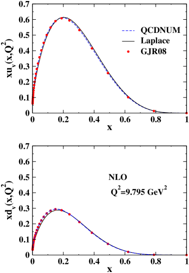
Figure 1: (Color online) Our results for the non-singlet distribution, $xu_{v}(x,Q^{2})$ and $xd_{v}(x,Q^{2})$, using Eq.(31) and comparison with the global QCD analysis of GJR08. The $x$-space results from the QCD evolution package, QCDnum, are also presented (dashed line).

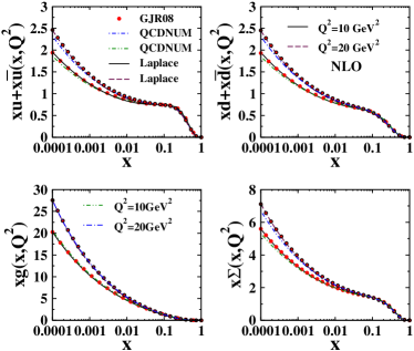
Figure 2: (Color online) Sea quarks and singlet distributions in comparison with the next-to-leading order results of GJR08 model. The gluon distribution are also shown. The solid-line correspond to Q² = 10 GeV² and the dashed-line correspond to Q² = 20 GeV². The results from the QCD evolution package, QCDnum, are also presented (dash-dotted and dash double-dotted lines).

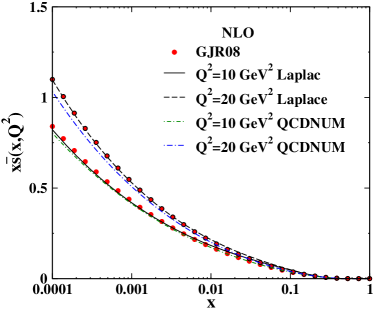
Figure 3: (Color online) The strange sea distribution $xs=x\overline{s}$ in comparison with the next-to-leading order results of GJR08 model. The solid line correspond to Q² = 10 GeV² and the dashed-line corresponds to Q² = 20 GeV². The results from the QCD evolution package, QCDnum, are also presented (dash-dotted and dash-double-dotted lines).

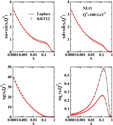
Figure 4: (Color online) Sea quarks, gluon and non-singlet distributions and comparison with the results from next-to-leading order KKT12 global QCD analysis at Q² = 100 GeV².

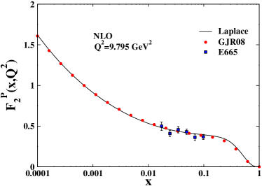
Figure 5: (Color online) The next-to-leading order approximation of the total proton structure function, $F_{2}^{\rm p,total}(x,Q^{2})$, as a function of $x$ at Q² = 9.795 GeV². The input distributions are obtained from the GJR08 model Gluck:2007ck . Here the straight line represents our result, using the Laplace transform technique, and the red circles represent the proton structure function arising from the GJR08 global QCD analysis. A comparison with the E665 experimental data Adams:1996gu is also shown.

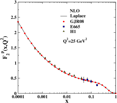
Figure 6: (Color online) The next-to-leading order approximation of the total proton structure function, $F_{2}^{\rm p,total}(x,Q^{2})$, as a function of $x$ at Q² = 25 GeV². The input distributions are obtained from the GJR08 model Gluck:2007ck . Here the straight line represents our result, using the Laplace transform technique, and the red circles represent the proton structure function arising from the GJR08 global QCD analysis. The square and up-triangle signs represent the the E665 experimental data Adams:1996gu and H1 inclusive deep inelastic neutral current data Aaron:2009kv , respectively.

VI The results of Laplace transformation technique

In this section, we present our results that have been obtained for the parton distribution functions and proton structure function $F_{2}^{p}(x,Q^{2})$ using the Laplace transformation technique to find an analytical solution for the DGLAP evolution equations. We obtain the valence quark distributions, $xu_{v}(x,Q^{2})$ and $xd_{v}(x,Q^{2})$, using Eq.(31) and compare them with the next-to-leading order GJR08 results. Since the GJR08 Collaboration started their evolution at Q${}_{0}^{2}$ = 2 GeV², we used $F_{\rm NS}^{0}$, $F_{\rm S}^{0}$ and $G^{0}$ constructed from their values at Q${}_{0}^{2}$ in Eq.(33). The results for the evolved non-singlet distributions are depicted in Fig. 1. To double check and indicate the sufficient precision of our analysis, we have also used the QCD evolution package, QCDnum Botje:2010ay and linked it to the LHAPDF Buckley:2014ana package for the GJR08 PDFs, which directly render the parton densities in $x$ space. As can be seen from the related figures, a good agreement between our results and the other ones exist. It indicates the evolution works well beyond the charm quark mass threshold, Q² > Q${}_{0}^{2}$ ($\approx m_{c}^{2}$ = 2 GeV²). In this figure the straight line represents the solution resulting from the Laplace transform technique and the red circles represent the valance quark distributions from GJR08 global QCD analysis. The dashed line indicates the results, arising out from QCDnum evolution package. One can conclude that the agreement, over the large span of $0<x<1$, is quite striking. The accuracy of the present analysis has been investigated and is typically better than about 1 part in 10⁵ at small and large values of Bjorken $x$ for the up-valence quark distribution $xu_{v}$. For the down-valence quark distribution $xd_{v}$, disagreements between our calculation and the GJR08 results are less than 1–2% for $0<x<0.2$.

In Fig. 2, the results for sea quark and singlet distributions are shown and compared with the next-to-leading order analysis of the GJR08 model as well as QCDnum evolution package. However some researchers are reporting the singlet solution rather than the individual distribution for sea quarks, but following the technique which was introduced in Furmanski:1980cm ; Furmanski:1981ja , it is possible to present separately the see quark distributions. The analytical solution for the gluon distribution, $G(x,Q^{2})=xg(x,Q^{2})$, is also shown. All distributions are obtained from Eq.(III) in $(s,\tau)$ space and then converted to the ($x$, Q²) space, using the convolution integrals in Eq.(III). The results indicated by the solid line correspond to Q² = 10 GeV² and the ones indicated by the dashed line correspond to Q² = 20 GeV². The strange sea distribution $xs=x\overline{s}$ and its comparison with the next-to-leading order results of the GJR08 model are also shown in Fig. 3 at Q² = 10 GeV² and Q² = 20 GeV². This figure indicates that the obtained results from the present analysis based on the Laplace transform technique are in good agreement with the ones obtained by global QCD analysis of GJR08 for the parton distribution functions and also the obtained results from the QCD evolution package, QCDnum. One can conclude from Figs. 2 and  3 that the agreements between our results and GJR08 global analysis are excellent over the entire range of momentum fraction-$x$ and the virtuality Q². We found slightly disagreements between $x$-space results calculated from the QCDnum package and the GJR08 analysis which are 1.5–2% for all parton species except for the gluon distribution. It is clear from the mentioned plots that, over the enormous Q² and $x$ spans, our analytic solutions are in satisfactory agreement with the GJR08 analysis.

A detailed comparison has also been shown with the next-to-leading order results from the KKT12 global QCD analysis and depicted in Fig. 4. In this figure our analytical solution based on the Laplace transform technique is presented for sea and singlet distributions as well as for the gluon distribution $G(x,Q^{2})=xg(x,Q^{2})$ at Q² = 100 GeV². The analytical solution arises from Eq.(III) which is related to the KKT12 initial distributions at Q${}_{0}^{2}$ = 2 GeV².

The results of analytical solutions for all parton distribution functions clearly show significant agreement over a wide range of $x$ and Q² variables. The only serious disagreements which we found between our calculations and the KKT12 results are for $xu+x\bar{u}$ and $xd+x\bar{d}$ distributions, which are smaller than 2–2.5% at $0.01<x<0.1$.

As a numerical illustration of our analytical approaches at the next-to-leading order approximation of the total proton structure function, $F_{2}^{p}(x,Q^{2})$, we compare our results with the GJR08 proton structure function and depict them in Figs. 5 and 6. A comparison with E665 data at fixed-target experiments  Adams:1996gu and H1 inclusive deep inelastic neutral current data Aaron:2009kv are also shown there. The results for the total proton structure function $F_{2}^{\rm p,total}(x,Q^{2})$ have been presented as a function of $x$ (both for large and small $x$) at Q² = 9.795 and 25 GeV². It is seen that our analytical solutions based on the inverse Laplace transform technique at the NLO approximation for the proton structure function over a wide range of $x$ and Q² values correspond well with the experimental data and the QCD analysis performed by GJR08 analysis. One can conclude that, in spite of small disagreement for the parton densities, we found a satisfactory agreement for the proton structure function over a wide range of $x$ and Q². The overall agreement is found to be 1 part in 10⁵.

Based on our obtained results for the next-to-leading order proton structure function, $F_{2}^{p}(x,Q^{2})$, and its good agreement with other theoretical models as well as experimental data, one can evaluate the parton distributions functions at the input scale Q${}_{0}^{2}$ by performing a global QCD fit to the all available and up-to-date DIS and hadron collision data, using the Jacobi polynomials approach. We plan to present our detailed QCD analysis based on the analytical calculation in the next section.

VII Jacobi polynomials technique for the DIS analysis

Global analysis of deep-inelastic scattering (DIS) data in the framework of QCD provides us with new knowledge of hadron physics and serves as a test of reliability of our theoretical understanding of the hard scattering of leptons and hadrons. Various QCD analyses, both for polarized and un-polarized case, can be constructed using all available data from fixed-target experiments, DIS data and the precise data from hadron colliders. For further literature on various PDFs models, we refer the reader to review articles Carrazza:2016htc ; Harland-Lang:2014zoa ; Mangano:2016jyj ; Pennington:2016dpj ; Dulat:2015mca ; Jimenez-Delgado:2014twa ; Carrazza:2015hva ; Rojo:2015acz ; DeRoeck:2011na ; Accardi:2016qay ; McNulty:2016xtv ; Accardi:2016ndt . The kinematics spanned by each DIS data set used in our fit are described in Secs. VII.

We shall focus here on the non-singlet (NS) structure functions, $F_{2}^{\rm NS}(x,Q^{2})$, with their corresponding Laplace $s$-space moments ${\cal M}^{\rm NS}(s,Q^{2})$ in order to perform a QCD analysis of deep inelastic scattering data up to the next-to-leading order (NLO). Based on a popular parametrization for the parton distribution functions (PDFs), we apply the Jacobi polynomial formalism. We consider a wide range of DIS data corresponding the momentum transfer from low Q${}_{0}^{2}\gtrsim 2\,{\rm GeV}^{2}$ to high Q${}^{2}\sim 30000\,{\rm GeV}^{2}$ where the approach still works reasonably still works. In this section, we first give an introductory description of the Jacobi polynomial approach, as the method of our QCD analysis for the non singlet (NS) structure functions and the procedure of the QCD fit to the data.

In the common $\overline{MS}$ factorization scheme, one can obtained the relevant $F_{2}$ structure function up to NLO from the combination of non-singlet, flavour singlet and gluon contributions of Eqs.(43–V).

In Laplace $s$ space, the combinations of parton densities at the valence region $x\geq 0.3$ for the proton structure function ${\cal M}_{2}^{p}$ in NLO can be written as:

$${\cal M}_{2}^{p}(s,\tau) = \left(\frac{4}{9}u_{v}(s)+\frac{1}{9}d_{v}(s)\right)\times$$ (48)

$$\left(1+\frac{\tau}{4\pi}C_{q}^{(1)}(s)\right)e^{\tau\Phi_{\rm NS}(s)}$$

In the above region, the combinations of parton densities for the deuteron structure function ${\cal M}_{2}^{d}$ are also given by,

$${\cal M}_{2}^{d}(s,\tau) = \frac{5}{18}\,(u_{v}(s)+d_{v}(s))\times\,,$$ (49)

$$\left(1+\frac{\tau}{4\pi}C_{q}^{(1)}(s)\right)e^{\tau\Phi_{\rm NS}(s)}\,,$$

where $d=\frac{p+n}{2}$. In the region of $x\leq 0.3$ for the difference of proton ${\cal M}_{2}^{p}$ and deuteron ${\cal M}_{2}^{d}$ data, we use:

$${\cal M}_{2}^{\rm NS}(s,\tau) \equiv 2({\cal M}_{2}^{p}-{\cal M}_{2}^{d})(s,\tau)$$ (50)

$$= \left(\frac{1}{3}\,(u_{v}-d_{v})(s)+\frac{2}{3}\,(\bar{u}-\bar{d})(s)\right)\times\leavevmode\nobreak\$$

$$\left(1+\frac{\tau}{4\pi}C_{q}^{(1)}(s)\right)e^{\tau\Phi_{\rm NS}(s)}$$

Since sea quarks can not be neglected for $x$ smaller than about 0.3, in our calculation we suppose the $\bar{d}-\bar{u}$ distribution from JR14 Jimenez-Delgado:2014twa at Q${}_{0}^{2}$ = 2 GeV² to be

$$x(\bar{d}-\bar{u})(x,Q_{0}^{2})=37.0x^{2.2}(1-x)^{19.2}(1+2.1\sqrt{x})\,,$$ (51)

As we mentioned at the beginning of this section, the method we have employed is using the Jacobi polynomials expansion of the structure functions. The details of the Jacobi polynomial approach are presented in our previous work Khorramian:2009xz . Here we outline a brief review of this method. According to this approach, using the Jacobi polynomial moments $a_{n}(Q^{2})$, one can reconstruct the structure function as,

$$xf(x,Q^{2})=x^{\beta}(1-x)^{\alpha}\sum_{n=0}^{\rm N_{max}}a_{n}(Q^{2})\Theta_{n}^{\alpha,\beta}(x)\,,$$ (52)

where ${\rm N_{max}}$ is the number of polynomials and $\Theta_{n}^{\alpha,\beta}(x)$ are the Jacobi polynomials of order $n$,

$$\Theta_{n}^{\alpha,\beta}(x)=\sum_{j=0}^{n}\,c_{j}^{(n)}{(\alpha,\beta)}\,x^{j}\,,$$ (53)

in which $c_{j}^{(n)}{(\alpha,\beta)}$ are the coefficients that are expressed through $\Gamma$ functions and satisfy the orthogonality relation with the weight $w^{\alpha,\beta}=x^{\beta}(1-x)^{\alpha}$ as follows

$$\int_{0}^{1}dx\,x^{\beta}(1-x)^{\alpha}\Theta_{m}^{\alpha,\beta}(x)\Theta_{n}^{\alpha,\beta}(x)=\delta_{mn}\,.$$ (54)

Using the above equations, we can relate the proton, neutron and non singlet structure functions with their Laplace $s$-space moments,

$$F_{2}^{\rm p,d,NS}(x,Q^{2}) = x^{\beta}(1-x)^{\alpha}\sum_{n=0}^{\rm N_{max}}\Theta_{n}^{\alpha,\beta}(x)$$

$$\times \sum_{j=0}^{n}\,c_{j}^{(n)}{(\alpha,\beta)}{\cal M}_{2}^{\rm p,d,NS}(s=j+1,Q^{2})\,,$$

where ${\cal M}_{2}^{\rm p,d,NS}(s,Q^{2})$ are the moments in Laplace $s$ space presented in Eqs.(48–50) for the proton, neutron and non-singlet structure functions. Here the Q² dependence of the structure functions will be provided by the Q² dependence of their moments in the Laplace-$s$ space. We consider ${\rm N_{max}}$ to be 9, $\alpha$ to be 3.0 and $\beta$ to be 0.7 to achieve the fastest convergence of the above series Khorramian:2009xz ; Krivokhizhin:1987rz ; Krivokhizhin:1990ct .

VII.1 Method of the QCD analysis

In this section, we present the details of the analysis which our analysis is based. We begin with a short discussion of the parametrization chosen for the various flavour PDFs. We then present a detailed discussion on the data set used and kinematic cuts applied. The method of the minimizations also will be discussed. Then we present the results of the analysis and describe the approach taken in this analysis.

PDF parametrizations

For the parametrization of the PDFs at the input scale Q${}^{2}_{0}$, chosen here to be 2 GeV², standard five-parameter form is adopted for valence parton species $f$,

$$xu_{v}(x,Q_{0}^{2}) = {\cal N}_{u}x^{\alpha_{u}}(1-x)^{\beta_{u}}(1+\gamma_{u}\sqrt{x}+\eta_{u}x)\,,$$

$$xd_{v}(x,Q_{0}^{2}) = {\cal N}_{d}x^{\alpha_{d}}(1-x)^{\beta_{d}}(1+\gamma_{d}\sqrt{x}+\eta_{d}x)\,.$$

This form applies to the up-valence $xu_{v}=xu-x\bar{u}$ and down-valence $xd_{v}=xd-x\bar{d}$ distributions. The normalization factors, ${\cal N}_{u}$ and ${\cal N}_{d}$, will be fixed by $\int_{0}^{1}u_{v}dx=2$ and $\int_{0}^{1}d_{v}dx=1$, respectively. In the Laplace $s$ space, the normalizations ${\cal N}_{u}$ and ${\cal N}_{d}$ are fixed by ${\cal L}[e^{-v}u_{v}(e^{-v});s=0]=2$ and ${\cal L}[e^{-v}d_{v}(e^{-v});s=0]=1$, respectively.

Data sets

Our valence PDFs are obtained by fitting to a global database of over 572 data points from a variety of high energy scattering processes. The data sets used in this analysis are listed in Table. 1. These include deep-inelastic scattering data from BCDMS Benvenuti:1989fm ; Benvenuti:1989rh ; Benvenuti:1989gs , SLAC Whitlow:1991uw and NMC Arneodo:1996qe ; Arneodo:1995cq experiments. The BCDMS data were collected at CERN and both proton and deuterium targets were used in the same experiment. These data sets facilitate flavor separation of PDFs at large $x$. The NMC experiment was also performed at CERN. The NMC data span lower values of $x$ and Q² and, due to the better coverage of the small-$x$ region, those data are also sensitive to the isospin asymmetry in the sea distribution.

The DIS data from H1 H1 and ZEUS ZEUS Collaborations are also included. New data sets from combined measurement of H1 and ZEUS Collaborations at HERA for the inclusive $e^{\pm}p$ scattering cross sections are also added Aaron:2009aa . As one can see from Table. 1, we use three data samples: for $F_{2}^{p}(x,Q^{2})$ and $F_{2}^{d}(x,Q^{2})$ in the valence quarks regions $x\geq 0.3$ and for $F_{2}^{\rm NS}(x,Q^{2})=2(F_{2}^{p}(x,Q^{2})-F_{2}^{d}(x,Q^{2}))$ in the region of $x<0.3$. Before the fitting process, we apply different cuts on data samples in order to widely eliminate the higher twist (HT) effects. Cuts on the kinematic coverage of the DIS data have been made for Q${}^{2}>4$ GeV² and on the hadronic mass of $W^{2}>12.5$. An additional cut on the BCDMS data ($y>0.35$) and on the NMC data ($Q^{2}>8$ GeV²) was also applied. The DIS data used in our fit and the number of data points for each experiment after the cuts are listed in Table  1. The numbers of reduced data points by the additional cuts are given in the fifth column of the table. This reduces the number of data points from 467 to 248 for $F_{2}^{p}(x,Q^{2})$, from 232 to 159 for $F_{2}^{d}(x,Q^{2})$ and from 208 to 165 for $F_{2}^{\rm NS}(x,Q^{2})$.

Table 1: Data sets used in our analysis, with the corresponding number of data points (a) $F_{2}^{p}(x,Q^{2})$, (b) $F_{2}^{d}(x,Q^{2})$, and (c) $F_{2}^{\rm NS}(x,Q^{2})$ for the non-singlet QCD analysis with their $x$ and Q² ranges. The name of different data sets, and range of $x$ and Q² are given in the three first columns. The normalization shifts are also listed in the last column. The details of corrections to data and the kinematic cuts applied on data are contained in the text.

Experiment	$x$	Q${}^{2},{\rm GeV}^{2}$	$F_{2}^{p}$	$F_{2}^{p}\leavevmode\nobreak\ {\rm cuts}$	${\cal N}$
BCDMS (100)	0.35–0.75	11.75–75.00	51	29	0.9984
BCDMS (120)	0.35–0.75	13.25–75.00	59	32	0.9968
BCDMS (200)	0.35–0.75	32.50–137.50	50	28	0.9986
BCDMS (280)	0.35–0.75	43.00–230.00	49	26	1.005
NMC (comb)	0.35–0.50	7.00–65.00	15	14	0.9996
SLAC (comb)	0.30–0.62	7.30–21.39	57	57	1.0000
H1 (hQ2)	0.40–0.65	200–30000	26	26	1.0015
ZEUS (hQ2)	0.40–0.65	650–30000	15	15	1.0000
H1 (comb)	0.40–0.65	90–30000	145	21	1.0000
Proton			467	248

(a) $F_{2}^{p}(x,Q^{2})$ data points.
Experiment $x$ Q${}^{2},{\rm GeV}^{2}$ $F_{2}^{d}$ $F_{2}^{d}\leavevmode\nobreak\ {\rm cuts}$ ${\cal N}$ BCDMS (120) 0.35–0.75 13.25–99.00 59 32 1.0069 BCDMS (200) 0.35–0.75 32.50–137.50 50 28 1.0048 BCDMS (280) 0.35–0.75 43.00–230.00 49 26 1.0038 NMC (comb) 0.35–0.50 7.00–65.00 15 14 0.9987 SLAC (comb) 0.30–0.62 10.00–21.40 59 59 0.9961 Deuteron 232 159
(b) $F_{2}^{d}(x,Q^{2})$ data points.
Experiment $x$ Q${}^{2},{\rm GeV}^{2}$ $F_{2}^{\rm NS}$ $F_{2}^{\rm NS}\leavevmode\nobreak\ {\rm cuts}$ ${\cal N}$ BCDMS (120) 0.070–0.275 8.75–43.00 36 30 0.9987 BCDMS (200) 0.070–0.275 17.00–75.00 29 28 0.9929 BCDMS (280) 0.100–0.275 32.50–115.50 27 26 0.9997 NMC (comb) 0.013–0.275 4.50–65.00 88 53 1.0002 SLAC (comb) 0.153–0.293 4.18–5.50 28 28 1.0010 Non-singlet 208 165
(c) $F_{2}^{\rm NS}(x,Q^{2})$ data points.

Statistical procedures

Agreement between the data sets and our theory predictions is quantified by the following $\chi^{2}_{\rm global}$ functional:

$$\chi^{2}_{\rm global}=\sum_{n=1}^{N_{\rm exp}}w_{n}\,\chi^{2}_{n}\,,$$ (57)

in which

$$\chi_{n}^{2} = \left(\frac{1-{\cal N}_{n}}{\Delta{\cal N}_{n}}\right)^{2}+\sum_{i=1}^{N^{\rm data}}\left(\frac{{\cal N}_{n}\,F_{2,i}^{\rm Data}-F_{2,i}^{\rm Theory})^{2}}{{\cal N}_{n}\,\Delta F_{2,i}^{\rm Data}}\right)^{2}$$ (58)

where $F_{2}^{\rm Data}$ and $F_{2}^{\rm Theory}$ stand for the measurements and theory predictions, respectively. $\Delta F_{2}^{\rm Data}$ is the measurements uncertainty (statistical and systematic combined in quadrature) and $i$ stands for $i$th data point in the fit. $\Delta{\cal N}_{n}$ is the experimental normalization uncertainty and ${\cal N}_{n}$ is the overall normalization factor which should be obtained from the fit to the data and then kept fixed. The minimization of the above $\chi^{2}_{\rm global}$ value to determine the best fit parameters of the valence parton distributions is done using the CERN program MINUIT James:1975dr . The value of $\chi^{2}/{\rm n.d.f}$ computed according to Eq.(57) for the used data sets is given in Table 2. The description quality is good enough for all data. This value is comparable to 1, therefore, the data can be easily accommodated in our fit. The uncertainties on the observables and on the PDFs throughout this paper, are computed using well-known Hessian error propagation, as outlined in Refs. Pumplin:2001ct ; Martin:2002aw ; Martin:2009iq ; Accardi:2016qay ; Owens:2012bv ; Accardi:2016ndt ; Khanpour:2016pph ; Shahri:2016uzl , with $\Delta\chi^{2}=5.86$, which corresponds to a 68% confidence level (C.L.) in the ideal Gaussian statistics.

VII.2 Target mass corrections (TMCs)

It is important to consider all sources of corrections in a QCD analysis which may contribute to a comparable magnitude, such as target mass corrections (TMCs) Georgi:1976ve ; Mirjalili:2012zz . In this section, we will focus on the target mass corrections, which formally are subleading $1/Q^{2}$ corrections to leading twist structure functions. Their effects are important at large value of $x$ and moderate $Q^{2}$, which coincides with the region where parton distribution functions (PDFs) are not very well determined. Consequently, a reliable perturbative QCD based analysis which includes data in the low-$Q^{2}$ region, demands an accurate description of the TMCs. To study the effect of TMCs, we follow the method presented in Refs. Georgi:1976ve ; Gluck:2006yz ; Steffens:2012jx ; Khorramian:2009xz to determine the analytical form in Laplace $s$-space. The moments of flavor non singlet structure functions in the presence of TMCs and in the Laplace $s$ space have the following form

$${\cal M}_{2,{\rm TMC}}^{k}(s,Q^{2})\equiv{\cal L}[{\cal M}_{2,{\rm TMC}}^{k}(e^{-v},Q^{2};s)]\,$$

$$={\cal M}_{2}^{k}(s,Q^{2})+\frac{s(s-1)}{s+2}\left(\frac{m_{N}^{2}}{Q^{2}}\right)\,{\cal M}_{2}^{k}(s+2,Q^{2})$$

$$+\frac{\Gamma(s+3)^{2}}{2\Gamma(s-1)\Gamma(s+5)}\left(\frac{m_{N}^{2}}{Q^{2}}\right)^{2}\,{\cal M}_{2}^{k}(s+4,Q^{2})$$

$$+\frac{\Gamma(s+4)\Gamma(s+5)}{6\Gamma(s-1)\Gamma(s+7)}\left(\frac{m_{N}^{2}}{Q^{2}}\right)^{3}\,{\cal M}_{2}^{k}(s+6,Q^{2})$$

$$+\frac{\Gamma(s+5)\Gamma(s+7)}{24\Gamma(s-1)\Gamma(s+9)}\left(\frac{m_{N}^{2}}{Q^{2}}\right)^{4}\,{\cal M}_{2}^{k}(s+8,Q^{2})$$

$$+{\cal{O}}\left(\frac{m_{N}^{2}}{Q^{2}}\right)^{5}\,,$$ (59)

where higher powers $(m_{\rm N}^{2}/Q^{2})^{n}$ ($n\geqslant 2$) are negligible for the relevant $x<0.8$ region. Consequently we can neglect these higher order parts. By inserting Eq.(VII.2) into Eq.(52), one can obtain

$$F_{2}^{k,{\rm TMC}}(x,Q^{2}) = x^{\beta}(1-x)^{\alpha}\sum_{n=0}^{\rm N_{max}}\Theta_{n}^{\alpha,\beta}(x)$$

$$\times \sum_{j=0}^{n}\,c_{j}^{(n)}{(\alpha,\beta)}\,{\cal M}_{2,{\rm TMC}}^{k}(j+1,Q^{2})\,.$$

In this equation ${\cal M}_{2,{\rm TMC}}^{k}(j+1,Q^{2})$ are the moments determined by Eq.(VII.2). The effects of TMCs on the PDFs and the corresponding observables will be illustrated in Sec. VII.4.

VII.3 Higher twist (HT) corrections

In addition to the important role played by TMCs at large values of $x$ and moderate $Q^{2}$, the effects of higher twist (HT) corrections are also significant Abt:2016vjh ; Jimenez-Delgado:2013boa ; Leader:2006xc ; Nath:2016phi ; Wei:2016far . Consequently, in the context of parton distribution analyses, the study of higher twists is also important in its own right. In addition to the kinematic cuts ($Q^{2}\geq 4$ GeV², $W^{2}\geq 12.5$ GeV²) we apply in our analysis, we also take into account higher twist corrections to the proton $F_{2}^{p}(x,Q^{2})$ and deuteron structure functions $F_{2}^{d}(x,Q^{2})$ for the kinematic region $Q^{2}\geq 4{\rm GeV}^{2},4<W^{2}<12.5{\rm GeV}^{2}$. For this purpose, we extrapolate our QCD fit results to this region.

In practice, higher twist contributions are usually parameterized independently from the leading twist one with some function of $x$, which is typically polynomial in $x$. In the region where the power corrections are non-negligible for the case of the DIS data, they are defined within an entirely phenomenologically motivated ansatz, as follows:

$$F_{2}^{\rm HT}(x,Q^{2})={\cal O}_{\rm TMC}[F_{2}^{\rm TMC}(x,Q^{2})]\cdot\left(1+\frac{h(x,Q^{2})}{Q^{2}[{\rm GeV}^{2}]}\right)\,,$$

where $F_{2}^{\rm TMC}(x,Q^{2})$ are given by Eq.(VII.2). In the above equation, the operation ${\cal O}_{\rm TMC}[...]$ denotes taking the target mass corrections of the twist–2 contributions to the respective structure function. As we mentioned, the coefficients $h(x,Q^{2})$ are determined in bins of $x$ and Q² and are then averaged over Q². The $x$-shape of the higher twist contributions is defined by the following expression,

$$h(x)=\alpha\left(\frac{x^{\beta}}{1-x}-\gamma\right)\,.$$ (62)

This choice of $h(x,Q^{2})$ provides sufficient flexibility of the higher twist terms with respect to the data analyzed. To perform higher twist QCD analysis of the non-singlet world data, we consider the $Q^{2}\geq 4\,{\rm GeV}^{2},4<W^{2}<12.5\,{\rm GeV}^{2}$ cuts. The parameter values of the $h(x)$ function were fitted to the data simultaneously with the valence PDFs parameters and the value of $\Lambda_{\rm QCD}$. The corresponding parameter values are presented in Table. 3. One can see the sensitivity of the fit to the higher twist terms in Sec. VII.4.

VII.4 Results of QCD fit

In this section, we present the results of our global QCD analysis which is based on the analytical solution based on Laplace transform technique and Jacobi polynomials approach. The parameter values of the next-to-leading order non-singlet QCD fit at the input scale of Q${}_{0}^{2}=2\,{\rm GeV}^{2}$ are presented in Table. 2. The parameters values without error have been fixed after the first minimization since the present data do not constrain these parameters well enough. From the table, one can finds rather stable PDF central values. The value for $\alpha_{\rm s}^{\rm N_{f}=4}(Q_{0}^{2})$ has also been obtained from the fit. This result can be expressed in terms of $\alpha_{s}(M_{Z}^{2})$, which is correspond to $\alpha_{s}(M_{Z}^{2})=0.1173\pm 0.0011$.

Next-to-leading order (NLO) fit
$u_{v}$	$\alpha_{u}$	0.7108 $\pm$ 0.1295
	$\beta_{u}$	3.3595 $\pm$ 0.027
	$\gamma_{u}$	0.2979
	$\eta_{u}$	1.3440
$d_{v}$	$\alpha_{d}$	0.9467 $\pm$ 0.0261
	$\beta_{d}$	2.8468 $\pm$ 0.3130
	$\gamma_{d}$	1.1004
	$\eta_{d}$	-1.1330
$\alpha_{\rm s}^{\rm N_{f}=4}(Q_{0}^{2})$		0.3521 $\pm$ 0.0139
$\chi^{2}/{\rm n.d.f}$		521.303/563 = 0.92

Table 2: Parameter values of the NLO non-singlet QCD fit at Q${}_{0}^{2}=2\,{\rm GeV}^{2}$. The parameters values without error have been fixed after the first minimization.

The obtained valence-quarks PDFs themselves are displayed in Fig. 7 at the input scale of Q${}_{0}^{2}=2\,{\rm GeV}^{2}$ along with their $\Delta\chi^{2}_{\text{global}}=5.86$ (68 % C.L.) uncertainty bands computed with the Hessian approach, for $xu_{v}(x,Q_{0}^{2})$ and $xd_{v}(x,Q_{0}^{2})$. For comparison, we also show the results from BBG Blumlein:2006be , GJR08 Gluck:2008gs and up-to-date results from CJ15 Accardi:2016qay PDFs.

NLO
$h(x)$	$\alpha=1.089$	$\beta=1.132$	$\gamma=0.960$

Table 3: Parameter values of the NLO HT fit at Q${}_{0}^{2}=2\,{\rm GeV}^{2}$.

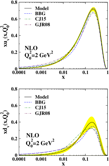
Figure 7: (Color online) The parton densities $xu_{v}$ and $xd_{v}$ at the input scale Q${}^{2}_{0}=2\,{\rm GeV}^{2}$. The uncertainties of our PDFs (yellow band) correspond to a 68% confidence level (C.L.) with $\Delta\chi^{2}_{\text{global}}=5.86$. The dashed line is the BBG PDF Blumlein:2006be ,the dashed-dotted line is the CJ15 PDF Accardi:2016qay and dashed-double-dotted line is the result from GJR08 Gluck:2008gs

For the higher value of Q² (=10 GeV²), we plot our $xu_{v}(x,Q^{2})$ and $xd_{v}(x,Q^{2})$ parton densities in Fig. 8. The valence-quark densities from several recent representative NLO global parametrizations including JR14 Jimenez-Delgado:2014twa , NNPDF2.3 Ball:2012cx and MMHT14 Harland-Lang:2014zoa are also shown for comparison. As this plot shows, the results of our analysis and from different parametrizations are in good agreement.

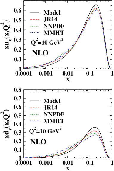
Figure 8: (Color online) The parton densities $xu_{v}(x,Q^{2})$ and $xd_{v}(x,Q^{2})$ at the scale of Q${}^{2}=10\,{\rm GeV}^{2}$. The dashed line is the JR14 PDFs Jimenez-Delgado:2014twa ,the dashed-dotted line is the NNPDF2.3 model Ball:2012cx , and the dashed-double-dotted line is the results from the MMHT14 group Harland-Lang:2014zoa .

The quality of the fit to the data is illustrated in Fig. 9, where the inclusive proton $F_{2}^{p}$ structure functions from BCDMS, SLAC, NMC, H1 and ZEUS are compared with our next-to-leading order fit as a function of Q² at approximately constant values of $x$. The data have been scaled by a factor $c$, from $c=1$ for $x=0.75$ to $c=15$ for $x=0.35$. The vertical arrowed line in the plot indicates the regions with $W^{2}>12.5\,{\rm GeV}^{2}$.

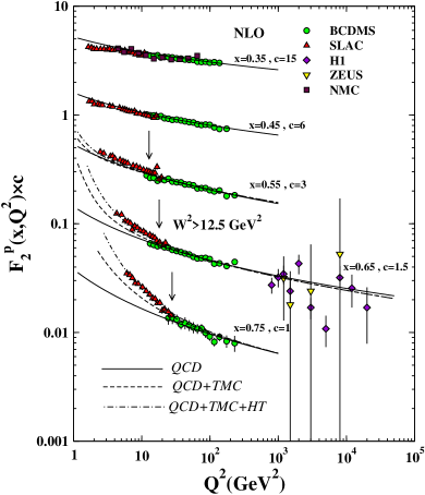
Figure 9: (Color online) Comparison of proton structure function $F^{p}_{2}$ data from BCDMS, SLAC, NMC, H1 and ZEUS with our theory predictions, as a function of Q² for fixed values of $x$. The pure QCD fit in next-to-leading order is shown as a solid line, the contributions from target mass corrections (TMCs) are shown as dashed line, and the higher twist (HT) correction is shown as a dashed-dotted line.

In Fig. 10, detailed comparisons of the deuteron structure function $F^{d}_{2}$ data from the BCDMS, SLAC and NMC experiments are shown with the theory predictions of our fit. The results have been plotted as a function of Q² with the corresponding $x$ ranges. The data have been scaled by a factor $c$, from $c=1$ for $x=0.75$ to $c=15$ for $x=0.35$.

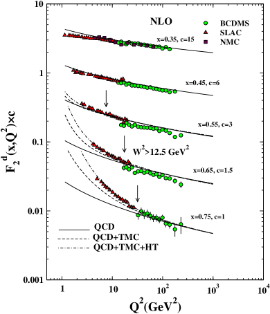
Figure 10: (Color online) Comparison of the structure function $F^{d}_{2}$ data from BCDMS, SLAC and NMC with our theory predictions, as a function of Q² for the fixed values of $x$. The pure QCD fit in next-to-leading order is shown by a solid line, the contributions from target mass corrections (TMCs) shown as a dashed line, and the higher twist (HT)correction is shown as a dashed-dotted line.

Comparisons to data from BCDMS and NMC experiments for the non-singlet structure function $F^{\rm NS}_{2}$ are shown in Fig. 11. The data have been scaled by a factor $c$, from $c=0.2$ for $x=0.275$ to $c=2.6$ for $x=0.0125$.

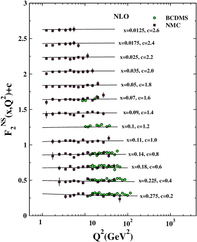
Figure 11: (Color online) Comparison of BCDMS and NMC data for the non-singlet structure function $F^{\rm NS}_{2}$ with our QCD predictions at next-to-leading order.

One can see that our theory predictions based on analytical solutions using Laplace transform and Jacobi polynomials provide a very good description of the data. When the effects of target mass corrections (TMCs) and higher-twist (HT) corrections are included, the agreement between theory prediction and the data become strikingly better. Figures. 9 and 10 clearly present this result. The agreements between the theory prediction for $F^{p}_{2}$ and $F^{d}_{2}$ structure functions (including TMCs and HT) and data, over several decades of Q² and $x$, are also excellent.

VIII Summary and conclusion

We presented the next-to-leading order decoupled analytical evolution equations for singlet $F_{\rm S}(x,Q^{2})$, gluon $G(x,Q^{2})$ and non-singlet $F_{\rm NS}(x,Q^{2})$ distributions, arising from the coupled DGLAP evolution equations in the Laplace s-space. We then rendered the results for valance quark distributions $xu_{v}$ and $xd_{v}$, the anti-quark distributions $x(\overline{d}+\overline{u})$ and $x\Delta=x(\overline{d}-\overline{u})$, the strange sea distribution $xs=x\overline{s}$ and the gluon distribution $xg$ initiated from KKT12 and GJR08 input parton distributions at Q${}_{0}^{2}$ = 2 GeV². In this work, we also calculated the proton structure function $F_{2}^{p}(x,Q^{2})$ using directly the Laplace transform technique, derived from corresponding analytical solutions for singlet $F_{2}^{\rm S}(x,Q^{2})$, $F_{2}^{\rm G}(x,Q^{2})$ and non-singlet $F_{2}^{\rm NS}(x,Q^{2})$ structure functions. To determine the proton structure function at any arbitrary Q² scale, we only need to know the initial distributions for singlet, gluon and non-singlet distributions at the input scale Q${}_{0}^{2}$. The method presented in this analysis enable us to achieve strictly analytical solution for parton densities and structure function in terms of the $x$ variable. We observed that the general solutions are in satisfactory agreements with the available experimental data and other parametrization models. In further research activities we hope to report the results of the Laplace transform technique to get analytical solutions for heavy quark contributions of the proton structure function. Extension of the current result to the higher next-to-next-to-leading order (NNLO) approximation is also a valuable task to pursue in future.

We also applied our approach to extract the initial valence-quarks densities $xu_{v}$ and $xd_{v}$ from fit to DIS data for the non-singlet sector. The Laplace transform technique and Jacobi polynomial approach were used to performed the analysis. When using this approach, the target mass corrections (TMCs) and higher twist (HT) effects are taken into account in the analysis. The obtained results are in satisfactory agreements with the DIS data and other phenomenological models. We hope to apply these techniques to a global fit of the experimental neutrino-nucleon structure function $xF_{3}(x,Q^{2})$ data in order to determine at the NLO approximation, the valence-quarks distributions $xu_{v}$ and $xd_{v}$, which can be used for the interpretation of results from future neutrino experiments.

In summary, there are various numerical methods to solve the DGLAP evolution equations to obtain the quarks and gluon parton distribution functions. In this paper we have shown that the methods of the Laplace transforms technique are also the reliable and alternative schemes to obtain the analytical solution of these equations. The advantage of using such a technique is that it enables us to achieve strictly analytical solutions for the proton distribution functions $F_{2}^{p}(x,Q^{2})$ in terms of the Bjorken-$x$ variable and virtuality Q².

Appendix A: The Laplace transforms of splitting functions at the NLO approximation

We present here the Laplace transforms of the splitting functions for quark and gluon sectors, denoted by $\Phi^{\rm NLO}$ and $\Theta^{\rm NLO}$ respectively at the next-to-leading order approximation which we used in Eqs.(III) and (29). We fixed the usual quadratic Casimir operators to their exact values, using $C_{A}=3$, ${\rm T_{F}}=f$ and $C_{F}=4/3$. The $\psi(s)$ is defined by $\psi(s)=\frac{d}{ds}{\rm ln}\Gamma(s)$ and $\gamma_{E}=0.577216$ is the Euler-Lagrange constant.

$$\Phi_{\rm{NS},qq}^{\rm{NLO}}=\hskip 398.33858pt\text{(A.1)}$$

$$C_{F}T_{F}\left(-\frac{2}{3(1+s)^{2}}-\frac{2}{9(1+s)}-\frac{2}{3(2+s)^{2}}+\frac{22}{9(2+s)}+\frac{20\left(\gamma_{E}+\psi(s+1)\right)}{9}+\frac{4}{3}\psi^{\prime}(s+1)\right)+$$

$$C_{F}{}^{2}\left(-\frac{1}{(1+s)^{3}}-\frac{5}{1+s}-\frac{1}{(2+s)^{3}}+\frac{2}{(2+s)^{2}}+\frac{5}{2+s}+\right.$$

$$\frac{2\left(\gamma_{E}+\frac{1}{1+s}+\psi(s+1)-(1+s)\psi^{\prime}(s+2)\right)}{(1+s)^{2}}+\frac{2\left(\gamma_{E}+\frac{1}{2+s}+\psi(s+2)-(2+s)\psi^{\prime}(s+3)\right)}{(2+s)^{2}}-$$

$$\left.4\left(\left(\gamma_{E}+\psi(s+1)\right)\psi^{\prime}(s+1)-\frac{1}{2}\psi^{\prime\prime}(s+1)\right)+3\psi^{\prime}(s+1)\right)+$$

$$C_{A}C_{F}\left(-\frac{1}{(1+s)^{3}}+\frac{5}{6(1+s)^{2}}+\frac{53}{18(1+s)}+\frac{\pi^{2}}{6(1+s)}-\frac{1}{(2+s)^{3}}+\right.$$

$$\frac{5}{6(2+s)^{2}}-\frac{187}{18(2+s)}+\frac{\pi^{2}}{6(2+s)}-\frac{67\left(\gamma_{E}+\psi(s+1)\right)}{9}+$$

$$\left.\frac{1}{3}\pi^{2}\left(\gamma_{E}+\psi(s+1)\right)-\frac{11}{3}\psi^{\prime}(s+1)-\psi^{\prime\prime}(s+1)\right)\,,$$

$$\Phi_{\rm{NS},q\bar{q}}^{\rm{NLO}}=\hskip 398.33858pt\text{(A.2)}$$

$$C_{F}\left(-\frac{C_{A}}{2}+C_{F}\right)$$

$$\left(-\frac{2}{(1+s)^{3}}-\frac{2}{(1+s)^{2}}+\frac{4}{1+s}+\frac{\pi^{2}}{3(1+s)}+\frac{2}{(2+s)^{3}}-\frac{2}{(2+s)^{2}}-\frac{8}{2+s}-\frac{\pi^{2}}{3(2+s)}+\frac{5}{3+s}-\right.$$

$$\frac{13}{9(4+s)}+\frac{25}{36(5+s)}-\frac{41}{100(6+s)}+\frac{4}{25(7+s)}-\left(\gamma_{E}+\psi\left(2+\frac{s}{2}\right)\right)-$$

$$\frac{1}{3}\pi^{2}\left(-\left(\gamma_{E}+\psi\left(\frac{1+s}{2}\right)\right)+\left(\gamma_{E}+\psi\left(1+\frac{s}{2}\right)\right)\right)+\left(\gamma_{E}+\psi\left(\frac{3+s}{2}\right)\right)+$$

$$4\left(-\left(\gamma_{E}+\psi\left(1+\frac{s}{2}\right)\right)+\left(\gamma_{E}+\psi\left(\frac{3+s}{2}\right)\right)\right)+\frac{4}{9}\left(-\left(\gamma_{E}+\psi\left(2+\frac{s}{2}\right)\right)+\left(\gamma_{E}+\psi\left(\frac{5+s}{2}\right)\right)\right)+$$

$$\frac{1}{4}\left(-\left(\gamma_{E}+\psi\left(3+\frac{s}{2}\right)\right)+\left(\gamma_{E}+\psi\left(\frac{5+s}{2}\right)\right)\right)+\frac{4}{25}\left(-\left(\gamma_{E}+\psi\left(3+\frac{s}{2}\right)\right)+\left(\gamma_{E}+\psi\left(\frac{7+s}{2}\right)\right)\right)+$$

$$\frac{1}{(1+s)^{3}}\left(-8+(1+s)\text{Ln}(16)+2(1+s)\psi\left(1+\frac{s}{2}\right)-2(1+s)\psi\left(\frac{1+s}{2}\right)-(1+s)^{2}\psi^{\prime}\left(1+\frac{s}{2}\right)+\right.$$

$$\left.(1+s)^{2}\psi^{\prime}\left(\frac{1+s}{2}\right)\right)-\frac{0.99984}{(2+s)^{3}}\left(\frac{16}{(1+s)^{2}}+\frac{12s}{(1+s)^{2}}+(2+s)\text{Ln}(16)-2(2+s)\psi\left(1+\frac{s}{2}\right)+2(2+s)\psi\left(\frac{1+s}{2}\right)+\right.\allowdisplaybreaks[1]$$

$$\left.(2+s)^{2}\psi^{\prime}\left(1+\frac{s}{2}\right)-(2+s)^{2}\psi^{\prime}\left(\frac{1+s}{2}\right)\right)-$$

$$\frac{1.9702}{(3+s)^{3}}\left(\frac{164+284s+188s^{2}+60s^{3}+8s^{4}}{(1+s)^{2}(2+s)^{2}}-4(3+s)\text{Ln}(2)-2(3+s)\psi\left(1+\frac{s}{2}\right)+\right.$$

$$\left.2(3+s)\psi\left(\frac{1+s}{2}\right)+(3+s)^{2}\psi^{\prime}\left(1+\frac{s}{2}\right)-(3+s)^{2}\psi^{\prime}\left(\frac{1+s}{2}\right)\right)-$$

$$\frac{1.801}{(4+s)^{3}}\left(\frac{2176+4392s+3504s^{2}+1408s^{3}+288s^{4}+24s^{5}}{(1+s)^{2}(2+s)^{2}(3+s)^{2}}+4(4+s)\text{Ln}(2)-\right.$$

$$\left.2(4+s)\psi\left(1+\frac{s}{2}\right)+2(4+s)\psi\left(\frac{1+s}{2}\right)+(4+s)^{2}\psi^{\prime}\left(1+\frac{s}{2}\right)-(4+s)^{2}\psi^{\prime}\left(\frac{1+s}{2}\right)\right)-$$

$$\frac{1.3242}{(5+s)^{3}}\left(\left.\left(57328+146144s+162160s^{2}+103728s^{3}+42144s^{4}+11160s^{5}+1880s^{6}+184s^{7}+8s^{8}\right)\right/\right.$$

$$\left((1+s)^{2}(2+s)^{2}(3+s)^{2}(4+s)^{2}\right)-4(5+s)\text{Ln}(2)-2(5+s)\psi\left(1+\frac{s}{2}\right)+$$

$$\left.2(5+s)\psi\left(\frac{1+s}{2}\right)+(5+s)^{2}\psi^{\prime}\left(1+\frac{s}{2}\right)-(5+s)^{2}\psi^{\prime}\left(\frac{1+s}{2}\right)\right)-$$

$$\frac{0.6348}{(6+s)^{2}}\left(\text{Ln}(16)-2\psi\left(4+\frac{s}{2}\right)+2\psi\left(\frac{7+s}{2}\right)+(6+s)\psi^{\prime}\left(4+\frac{s}{2}\right)-(6+s)\psi^{\prime}\left(\frac{7+s}{2}\right)\right)+$$

$$\frac{0.1398}{(7+s)^{2}}\left(\text{Ln}(16)+2\psi\left(4+\frac{s}{2}\right)-2\psi\left(\frac{9+s}{2}\right)-(7+s)\psi^{\prime}\left(4+\frac{s}{2}\right)+(7+s)\psi^{\prime}\left(\frac{9+s}{2}\right)\right)+$$

$$\left.\frac{1}{4}\left(\psi^{\prime\prime}\left(\frac{2+s}{2}\right)-\psi^{\prime\prime}\left(\frac{1+s}{2}\right)\right)\right)\,,$$

$$\Phi_{qq}^{\rm{NLO}}=\hskip 398.33858pt\text{(A.3)}$$

$$C_{F}T_{F}\left(\frac{40}{9s}-\frac{4}{(1+s)^{3}}-\frac{8}{3(1+s)^{2}}-\frac{38}{9(1+s)}-\frac{4}{(2+s)^{3}}-\frac{32}{3(2+s)^{2}}+\frac{130}{9(2+s)}-\frac{16}{3(3+s)^{2}}-\right.$$

$$\left.\frac{112}{9(3+s)}+\frac{20\left(\gamma_{E}+\psi(s+1)\right)}{9}+\frac{4}{3}\psi^{\prime}(s+1)\right)+$$

$$C_{F}^{2}\left(\frac{1}{(1+s)^{3}}-\frac{2}{(1+s)^{2}}-\frac{1}{1+s}-\frac{\pi^{2}}{3(1+s)}-\frac{2.999}{(2+s)^{3}}+\frac{8.289}{2+s}+\frac{\text{{``}3.9404{''}}}{(3+s)^{3}}-\frac{11.481}{3+s}-\right.$$

$$\frac{3.602}{(4+s)^{3}}+\frac{15.25}{4+s}+\frac{2.648}{(5+s)^{3}}-\frac{14.225}{5+s}-\frac{1.269}{(6+s)^{3}}+\frac{10.472}{6+s}+\frac{0.279}{(7+s)^{3}}-\frac{5.776}{7+s}+$$

$$\frac{2.548}{8+s}-\frac{1.0411}{9+s}+\frac{0.4327}{10+s}-\frac{0.136}{11+s}+\frac{0.0224}{12+s}+$$

$$\frac{1}{(1+s)^{3}}\left(-8+(1+s)\text{Ln}(16)+2(1+s)\psi\left(1+\frac{s}{2}\right)-2(1+s)\psi\left(\frac{1+s}{2}\right)-\right.$$

$$\left.(1+s)^{2}\psi^{\prime}\left(1+\frac{s}{2}\right)+(1+s)^{2}\psi^{\prime}\left(\frac{1+s}{2}\right)\right)-$$

$$\frac{0.999}{(2+s)^{3}}\left(\frac{16}{(1+s)^{2}}+\frac{12s}{(1+s)^{2}}+(2+s)\text{Ln}(16)-2(2+s)\psi\left(1+\frac{s}{2}\right)+2(2+s)\psi\left(\frac{1+s}{2}\right)+\right.$$

$$\left.(2+s)^{2}\psi^{\prime}\left(1+\frac{s}{2}\right)-(2+s)^{2}\psi^{\prime}\left(\frac{1+s}{2}\right)\right)-$$

$$\frac{1.9702}{(3+s)^{3}}\left(\frac{164+284s+188s^{2}+60s^{3}+8s^{4}}{(1+s)^{2}(2+s)^{2}}-4(3+s)\text{Ln}[2]-2(3+s)\psi\left(1+\frac{s}{2}\right)+\right.$$

$$\left.2(3+s)\psi\left(\frac{1+s}{2}\right)+(3+s)^{2}\psi^{\prime}\left(1+\frac{s}{2}\right)-(3+s)^{2}\psi^{\prime}\left(\frac{1+s}{2}\right)\right)-\allowdisplaybreaks[1]$$

$$\frac{1.801}{(4+s)^{3}}\left(\frac{2176+4392s+3504s^{2}+1408s^{3}+288s^{4}+24s^{5}}{(1+s)^{2}(2+s)^{2}(3+s)^{2}}+4(4+s)\text{Ln}[2]-\right.$$

$$\left.2(4+s)\psi\left(1+\frac{s}{2}\right)+2(4+s)\psi\left(\frac{1+s}{2}\right)+(4+s)^{2}\psi^{\prime}\left(1+\frac{s}{2}\right)-(4+s)^{2}\psi^{\prime}\left(\frac{1+s}{2}\right)\right)-$$

$$\frac{1.3242}{(5+s)^{3}}\left(\frac{57328+146144s+162160s^{2}+103728s^{3}+42144s^{4}+11160s^{5}+1880s^{6}+184s^{7}+8s^{8}}{(1+s)^{2}(2+s)^{2}(3+s)^{2}(4+s)^{2}}-\right.$$

$$4(5+s)\text{Ln}[2]-2(5+s)\psi\left(1+\frac{s}{2}\right)+2(5+s)\psi\left(\frac{1+s}{2}\right)+(5+s)^{2}\psi^{\prime}\left(1+\frac{s}{2}\right)-$$

$$\left.(5+s)^{2}\psi^{\prime}\left(\frac{1+s}{2}\right)\right)+\frac{2\left(\gamma_{E}+\frac{1}{1+s}+\psi(s+1)-(1+s)\psi^{\prime}(s+2)\right)}{(1+s)^{2}}+$$

$$\frac{2\left(\gamma_{E}+\frac{1}{2+s}+\psi(s+2)-(2+s)\psi^{\prime}(s+3)\right)}{(2+s)^{2}}-$$

$$\frac{0.6348}{(6+s)^{2}}\left(\text{Ln}(16)-2\psi\left(4+\frac{s}{2}\right)+2\psi\left(\frac{7+s}{2}\right)+(6+s)\psi^{\prime}\left(4+\frac{s}{2}\right)-(6+s)\psi^{\prime}\left(\frac{7+s}{2}\right)\right)+$$

$$\frac{0.1398}{(7+s)^{2}}\left(\text{Ln}(16)+2\psi\left(4+\frac{s}{2}\right)-2\psi\left(\frac{9+s}{2}\right)-(7+s)\psi^{\prime}\left(4+\frac{s}{2}\right)+(7+s)\psi^{\prime}\left(\frac{9+s}{2}\right)\right)-$$

$$\left.4\left(\left(\gamma_{E}+\psi(s+1)\right)\psi^{\prime}(s+1)-\frac{1}{2}\psi^{\prime\prime}(s+1)\right)+3\psi^{\prime}(s+1)\right)+$$

$$C_{A}C_{F}\left(-\frac{2}{(1+s)^{3}}+\frac{11}{6(1+s)^{2}}+\frac{17}{18(1+s)}+\frac{\pi^{2}}{3(1+s)}-\frac{0.00016}{(2+s)^{3}}+\frac{11}{6(2+s)^{2}}-\frac{10.39}{2+s}-\right.$$

$$\frac{1.97}{(3+s)^{3}}+\frac{5.74}{3+s}+\frac{1.801}{(4+s)^{3}}-\frac{7.625}{4+s}-\frac{1.32}{(5+s)^{3}}+\frac{7.112}{5+s}+\frac{0.634}{(6+s)^{3}}-\frac{5.23}{6+s}-\frac{0.139}{(7+s)^{3}}+$$

$$\frac{2.88}{7+s}-\frac{1.274}{8+s}+\frac{0.5205}{9+s}-\frac{0.216}{10+s}+\frac{0.068}{11+s}-\frac{0.0112}{12+s}-\frac{67\left(\gamma_{E}+\psi(s+1)\right)}{9}+$$

$$\frac{1}{3}\pi^{2}\left(\gamma_{E}+\psi(s+1)\right)-$$

$$\frac{1}{2(1+s)^{3}}\left(-8+(1+s)\text{Ln}(16)+2(1+s)\psi\left(1+\frac{s}{2}\right)-2(1+s)\psi\left(\frac{1+s}{2}\right)-\right.$$

$$\left.(1+s)^{2}\psi^{\prime}\left(1+\frac{s}{2}\right)+(1+s)^{2}\psi^{\prime}\left(\frac{1+s}{2}\right)\right)+$$

$$\frac{0.49992}{(2+s)^{3}}\left(\frac{16}{(1+s)^{2}}+\frac{12s}{(1+s)^{2}}+(2+s)\text{Ln}(16)-2(2+s)\psi\left(1+\frac{s}{2}\right)+2(2+s)\psi\left(\frac{1+s}{2}\right)+\right.$$

$$\left.(2+s)^{2}\psi^{\prime}\left(1+\frac{s}{2}\right)-(2+s)^{2}\psi^{\prime}\left(\frac{1+s}{2}\right)\right)+$$

$$\frac{0.9851}{(3+s)^{3}}\left(\frac{164+284s+188s^{2}+60s^{3}+8s^{4}}{(1+s)^{2}(2+s)^{2}}-4(3+s)\text{Ln}[2]-2(3+s)\psi\left(1+\frac{s}{2}\right)+\right.$$

$$\left.2(3+s)\psi\left(\frac{1+s}{2}\right)+(3+s)^{2}\psi^{\prime}\left(1+\frac{s}{2}\right)-(3+s)^{2}\psi^{\prime}\left(\frac{1+s}{2}\right)\right)+$$

$$\frac{0.9005}{(4+s)^{3}}\left(\frac{2176+4392s+3504s^{2}+1408s^{3}+288s^{4}+24s^{5}}{(1+s)^{2}(2+s)^{2}(3+s)^{2}}+4(4+s)\text{Ln}[2]-\right.$$

$$\left.2(4+s)\psi\left(1+\frac{s}{2}\right)+2(4+s)\psi\left(\frac{1+s}{2}\right)+(4+s)^{2}\psi^{\prime}\left(1+\frac{s}{2}\right)-(4+s)^{2}\psi^{\prime}\left(\frac{1+s}{2}\right)\right)+$$

$$\frac{0.6621}{(5+s)^{3}}\left(\frac{57328+146144s+162160s^{2}+103728s^{3}+42144s^{4}+11160s^{5}+1880s^{6}+184s^{7}+8s^{8}}{(1+s)^{2}(2+s)^{2}(3+s)^{2}(4+s)^{2}}-\right.$$

$$4(5+s)\text{Ln}[2]-2(5+s)\psi\left(1+\frac{s}{2}\right)+2(5+s)\psi\left(\frac{1+s}{2}\right)+(5+s)^{2}\psi^{\prime}\left(1+\frac{s}{2}\right)-$$

$$\left.(5+s)^{2}\psi^{\prime}\left(\frac{1+s}{2}\right)\right)+\frac{0.3174}{(6+s)^{2}}\left(\text{Ln}(16)-2\psi\left(4+\frac{s}{2}\right)+2\psi\left(\frac{7+s}{2}\right)+(6+s)\psi^{\prime}\left(4+\frac{s}{2}\right)-(6+s)\psi^{\prime}\left(\frac{7+s}{2}\right)\right)-$$

$$\frac{0.0699}{(7+s)^{2}}\left(\text{Ln}(16)+2\psi\left(4+\frac{s}{2}\right)-2\psi\left(\frac{9+s}{2}\right)-(7+s)\psi^{\prime}\left(4+\frac{s}{2}\right)+(7+s)\psi^{\prime}\left(\frac{9+s}{2}\right)\right)-\left.\frac{11}{3}\psi^{\prime}(s+1)-\psi^{\prime\prime}(s+1)\right)\,,$$

$$\Theta_{f}^{\rm{NLO}}=\hskip 398.33858pt\text{(A.4)}$$

$$C_{F}T_{F}\left(-\frac{2}{(1+s)^{3}}+\frac{1}{(1+s)^{2}}+\frac{14}{1+s}-\frac{2\pi^{2}}{3(1+s)}+\frac{4}{(2+s)^{3}}-\frac{4}{(2+s)^{2}}-\frac{29}{2+s}+\right.$$

$$\frac{4\pi^{2}}{3(2+s)}+\frac{20}{3+s}-\frac{4\pi^{2}}{3(3+s)}+\frac{4\left(\gamma_{E}+\psi(s+1)\right)}{1+s}-\frac{4\left(\gamma_{E}+\psi(s+2)\right)}{1+s}-$$

$$\frac{8\left(\gamma_{E}+\psi(s+2)\right)}{2+s}+\frac{8\left(\gamma_{E}+\psi(s+3)\right)}{3+s}+\frac{2\left(\pi^{2}+6\left(\gamma_{E}+\psi(s+1)\right){}^{2}+6\psi^{\prime}(s+1)\right)}{6+6s}-$$

$$\frac{4\left(\pi^{2}+6\left(\gamma_{E}+\psi(s+2)\right){}^{2}+6\psi^{\prime}(s+2)\right)}{12+6s}+$$

$$\left.\frac{4\left(\pi^{2}+6\left(\gamma_{E}+\psi(s+3)\right){}^{2}+6\psi^{\prime}(s+3)\right)}{18+6s}\right)+$$

$$C_{A}T_{F}\left(\frac{40}{9s}-\frac{4}{(1+s)^{3}}-\frac{2}{(1+s)^{2}}-\frac{4}{1+s}-\frac{8}{(2+s)^{3}}-\frac{16}{(2+s)^{2}}+\frac{54}{2+s}-\frac{4\pi^{2}}{3(2+s)}-\right.$$

$$\frac{88}{3(3+s)^{2}}-\frac{373}{9(3+s)}+\frac{58}{9(4+s)}-\frac{49}{36(5+s)}+\frac{247}{450(6+s)}-\frac{9}{50(7+s)}+$$

$$\frac{8}{25(8+s)}+\frac{8\left(\gamma_{E}+\psi(s+3)\right)}{2+s}-\frac{8\left(\gamma_{E}+\psi(s+4)\right)}{3+s}+$$

$$\frac{1}{(1+s)^{3}}\left(-8+(1+s)\text{Ln}(16)+2(1+s)\psi\left(1+\frac{s}{2}\right)-2(1+s)\psi\left(\frac{1+s}{2}\right)-\right.$$

$$\left.(1+s)^{2}\psi^{\prime}\left(1+\frac{s}{2}\right)+(1+s)^{2}\psi^{\prime}\left(\frac{1+s}{2}\right)\right)+$$

$$\frac{1}{(2+s)^{3}}2\left(\frac{16}{(1+s)^{2}}+\frac{12s}{(1+s)^{2}}+(2+s)\text{Ln}(16)-2(2+s)\psi\left(1+\frac{s}{2}\right)+\right.$$

$$\left.2(2+s)\psi\left(\frac{1+s}{2}\right)+(2+s)^{2}\psi^{\prime}\left(1+\frac{s}{2}\right)-(2+s)^{2}\psi^{\prime}\left(\frac{1+s}{2}\right)\right)-$$

$$\frac{1}{(3+s)^{3}}2\left(\frac{164+284s+188s^{2}+60s^{3}+8s^{4}}{(1+s)^{2}(2+s)^{2}}-4(3+s)\text{Ln}(2)-\right.$$

$$2(3+s)\psi\left(1+\frac{s}{2}\right)+2(3+s)\psi\left(\frac{1+s}{2}\right)+(3+s)^{2}\psi^{\prime}\left(1+\frac{s}{2}\right)-$$

$$\left.(3+s)^{2}\psi^{\prime}\left(\frac{1+s}{2}\right)\right)-\frac{2\left(\pi^{2}+6\left(\gamma_{E}+\psi(s+2)\right){}^{2}-6\psi^{\prime}(s+2)\right)}{6+6s}+$$

$$\frac{4\left(\pi^{2}+6\left(\gamma_{E}+\psi(s+3)\right){}^{2}-6\psi^{\prime}(s+3)\right)}{12+6s}-$$

$$\left.\frac{4\left(\pi^{2}+6\left(\gamma_{E}+\psi(s+4)\right){}^{2}-6\psi^{\prime}(s+4)\right)}{18+6s}\right)\,,$$

$$\Theta_{g}^{\rm{NLO}}=\hskip 398.33858pt\text{(A.5)}$$

$$C_{F}T_{F}\left(-\frac{40}{9s}+\frac{40}{9(1+s)}-\frac{32}{9(2+s)}+\frac{8\left(\gamma_{E}+\psi(s+1)\right)}{3s}-\frac{8\left(\gamma_{E}+\psi(s+2)\right)}{3(1+s)}+\right.$$

$$\left.\frac{4\left(\gamma_{E}+\psi(s+3)\right)}{3(2+s)}\right)+$$

$$C_{F}^{2}\left(-\frac{2}{(1+s)^{3}}-\frac{2}{(1+s)^{2}}-\frac{5}{2(1+s)}+\frac{1}{(2+s)^{3}}-\frac{7}{2(2+s)^{2}}-\frac{7}{2(2+s)}+\right.$$

$$\frac{6\left(\gamma_{E}+\psi(s+1)\right)}{s}-\frac{6\left(\gamma_{E}+\psi(s+2)\right)}{1+s}+\frac{5\left(\gamma_{E}+\psi(s+3)\right)}{2+s}-$$

$$\frac{\pi^{2}+6\left(\gamma_{E}+\psi(s+1)\right){}^{2}-6\psi^{\prime}(s+1)}{3s}+\frac{2\left(\pi^{2}+6\left(\gamma_{E}+\psi(s+2)\right){}^{2}-6\psi^{\prime}(s+2)\right)}{6+6s}-$$

$$\left.\frac{\pi^{2}+6\left(\gamma_{E}+\psi(s+3)\right){}^{2}-6\psi^{\prime}(s+3)}{12+6s}\right)+$$

$$C_{A}C_{F}\left(\frac{1}{s}+\frac{4}{(1+s)^{3}}+\frac{12}{(1+s)^{2}}-\frac{17}{9(1+s)}+\frac{2\pi^{2}}{3(1+s)}+\frac{2}{(2+s)^{3}}+\frac{5}{(2+s)^{2}}+\right.$$

$$\frac{10}{9(2+s)}+\frac{8}{3(3+s)^{2}}+\frac{31}{9(3+s)}+\frac{11}{36(4+s)}-\frac{119}{900(5+s)}-\frac{7}{200(6+s)}-$$

$$\frac{2}{25(7+s)}-\frac{22\left(\gamma_{E}+\psi(s+1)\right)}{3s}+\frac{22\left(\gamma_{E}+\psi(s+2)\right)}{3(1+s)}-\frac{17\left(\gamma_{E}+\psi(s+3)\right)}{3(2+s)}-$$

$$\frac{1}{s^{2}}\left(\text{Ln}(16)-2\psi\left(1+\frac{s}{2}\right)+2\psi\left(\frac{1+s}{2}\right)+s\psi^{\prime}\left(1+\frac{s}{2}\right)-s\psi^{\prime}\left(\frac{1+s}{2}\right)\right)-$$

$$\frac{1}{(1+s)^{3}}\left(-8+(1+s)\text{Ln}(16)+2(1+s)\psi\left(1+\frac{s}{2}\right)-2(1+s)\psi\left(\frac{1+s}{2}\right)-\right.$$

$$\left.(1+s)^{2}\psi^{\prime}\left(1+\frac{s}{2}\right)+(1+s)^{2}\psi^{\prime}\left(\frac{1+s}{2}\right)\right)-$$

$$\frac{1}{2(2+s)^{3}}\left(\frac{16}{(1+s)^{2}}+\frac{12s}{(1+s)^{2}}+(2+s)\text{Ln}(16)-2(2+s)\psi\left(1+\frac{s}{2}\right)+\right.$$

$$\left.2(2+s)\psi\left(\frac{1+s}{2}\right)+(2+s)^{2}\psi^{\prime}\left(1+\frac{s}{2}\right)-(2+s)^{2}\psi^{\prime}\left(\frac{1+s}{2}\right)\right)+$$

$$\frac{\pi^{2}+6\left(\gamma_{E}+\psi(s+1)\right){}^{2}-6\psi^{\prime}(s+1)}{3s}-\frac{4\left(1+\gamma_{E}s+s(\psi(s)-s\psi^{\prime}(s+1))\right)}{s^{3}}-$$

$$\frac{2\left(\pi^{2}+6\left(\gamma_{E}+\psi(s+2)\right){}^{2}-6\psi^{\prime}(s+2)\right)}{6+6s}+\frac{4\left(\gamma_{E}+\frac{1}{1+s}+\psi(s+1)-(1+s)\psi^{\prime}(s+2)\right)}{(1+s)^{2}}+$$

$$\frac{\pi^{2}+6\left(\gamma_{E}+\psi(s+3)\right){}^{2}-6\psi^{\prime}(s+3)}{12+6s}-\left.\frac{2\left(\gamma_{E}+\frac{1}{2+s}+\psi(s+2)-(2+s)\psi^{\prime}(s+3)\right)}{(2+s)^{2}}\right)\,,$$

$$\Phi_{g}^{\rm{NLO}}=\hskip 398.33858pt\text{(A.6)}$$

$$C_{F}T_{F}\left(\frac{4}{3s}-\frac{4}{(1+s)^{3}}+\frac{6}{(1+s)^{2}}-\frac{16}{1+s}-\frac{4}{(2+s)^{3}}+\frac{10}{(2+s)^{2}}+\frac{8}{2+s}+\frac{20}{3(3+s)}\right)+$$

$$C_{A}T_{F}\left(-\frac{46}{9s}+\frac{4}{3(1+s)^{2}}+\frac{58}{9(1+s)}+\frac{4}{3(2+s)^{2}}-\frac{38}{9(2+s)}+\frac{46}{9(3+s)}+\right.$$

$$\left.\frac{20\left(\gamma_{E}+\psi^{\prime}(s+1)\right)}{9}\right)+$$

$$C_{A}{}^{2}\left(\frac{2}{(1+s)^{3}}+\frac{25}{3(1+s)^{2}}-\frac{97}{18(1+s)}+\frac{\pi^{2}}{1+s}+\frac{\text{{``}6.{''}}}{(2+s)^{3}}-\frac{11}{3(2+s)^{2}}-\right.$$

$$\frac{2.476}{2+s}-\frac{\pi^{2}}{3(2+s)}-\frac{2.029}{(3+s)^{3}}+\frac{44}{3(3+s)^{2}}-\frac{7.395}{3+s}+\frac{\pi^{2}}{3(3+s)}-$$

$$\frac{1.801}{(4+s)^{3}}+\frac{4.708}{4+s}+\frac{1.324}{(5+s)^{3}}-\frac{6.564}{5+s}-\frac{0.635}{(6+s)^{3}}+\frac{4.926}{6+s}+\frac{0.139}{(7+s)^{3}}-$$

$$\frac{2.878}{7+s}+\frac{1.114}{8+s}-\frac{0.521}{9+s}+\frac{0.217}{10+s}-\frac{0.0683}{11+s}+\frac{0.0112}{12+s}-\frac{67\left(\gamma_{E}+\psi^{\prime}(s+1)\right)}{9}+$$

$$\frac{1}{3}\pi^{2}\left(\gamma_{E}+\psi^{\prime}(s+1)\right)-\frac{1}{s^{2}}\left(\text{Ln}(16)-2\psi\left(1+\frac{s}{2}\right)+2\psi\left(\frac{1+s}{2}\right)+s\psi^{\prime}\left(1+\frac{s}{2}\right)-s\psi^{\prime}\left(\frac{1+s}{2}\right)\right)-$$

$$\frac{1}{(1+s)^{3}}\left(-8+(1+s)\text{Ln}(16)+2(1+s)\psi\left(1+\frac{s}{2}\right)-2(1+s)\psi\left(\frac{1+s}{2}\right)-\right.$$

$$\left.(1+s)^{2}\psi^{\prime}\left(1+\frac{s}{2}\right)+(1+s)^{2}\psi^{\prime}\left(\frac{1+s}{2}\right)\right)-$$

$$\frac{1.99992}{(2+s)^{3}}\left(\frac{16+12s}{(1+s)^{2}}+(2+s)\text{Ln}(16)-2(2+s)\psi\left(1+\frac{s}{2}\right)+\right.$$

$$\left.2(2+s)\psi\left(\frac{1+s}{2}\right)+(2+s)^{2}\psi^{\prime}\left(1+\frac{s}{2}\right)-(2+s)^{2}\psi^{\prime}\left(\frac{1+s}{2}\right)\right)+$$

$$\frac{0.0149}{(3+s)^{3}}\left(\frac{164+284s+188s^{2}+60s^{3}+8s^{4}}{(1+s)^{2}(2+s)^{2}}-4(3+s)\text{Ln}(2)-\right.$$

$$2(3+s)\psi\left(1+\frac{s}{2}\right)+2(3+s)\psi\left(\frac{1+s}{2}\right)+(3+s)^{2}\psi^{\prime}\left(1+\frac{s}{2}\right)-$$

$$\left.(3+s)^{2}\psi^{\prime}\left(\frac{1+s}{2}\right)\right)-\frac{0.9005}{(4+s)^{3}}\left(\frac{2176+4392s+3504s^{2}+1408s^{3}+288s^{4}+24s^{5}}{(1+s)^{2}(2+s)^{2}(3+s)^{2}}+\right.$$

$$4(4+s)\text{Ln}(2)-2(4+s)\psi\left(1+\frac{s}{2}\right)+2(4+s)\psi\left(\frac{1+s}{2}\right)+\left.(4+s)^{2}\psi^{\prime}\left(1+\frac{s}{2}\right)-(4+s)^{2}\psi^{\prime}\left(\frac{1+s}{2}\right)\right)-$$

$$\frac{0.6621}{(5+s)^{3}}\left(\left(57328+146144s+162160s^{2}+103728s^{3}+42144s^{4}+11160s^{5}+\right.\right.$$

$$\left.1880s^{6}+184s^{7}+8s^{8}\right)/\left((1+s)^{2}(2+s)^{2}(3+s)^{2}(4+s)^{2}\right)-$$

$$4(5+s)\text{Ln}(2)-2(5+s)\psi\left(1+\frac{s}{2}\right)+2(5+s)\psi\left(\frac{1+s}{2}\right)+$$

$$\left.(5+s)^{2}\psi^{\prime}\left(1+\frac{s}{2}\right)-(5+s)^{2}\psi^{\prime}\left(\frac{1+s}{2}\right)\right)-\frac{4\left(1+\gamma_{E}s+s(\psi(s)-s\psi^{\prime}(s+1))\right)}{s^{3}}+$$

$$\frac{8\left(\gamma_{E}+\frac{1}{1+s}+\psi^{\prime}(s+1)-(1+s)\psi^{\prime}(s+2)\right)}{(1+s)^{2}}-\frac{4\left(\gamma_{E}+\frac{1}{2+s}+\psi(s+2)-(2+s)\psi^{\prime}(s+3)\right)}{(2+s)^{2}}+$$

$$\frac{4\left(\gamma_{E}+\frac{1}{3+s}+\psi(s+3)-(3+s)\psi^{\prime}(s+4)\right)}{(3+s)^{2}}-$$

$$\frac{0.3174}{(6+s)^{2}}\left(\text{Ln}(16)-2\psi\left(4+\frac{s}{2}\right)+2\psi\left(\frac{7+s}{2}\right)+(6+s)\psi^{\prime}\left(4+\frac{s}{2}\right)-\right.\allowdisplaybreaks[1]$$

$$\left.(6+s)\psi^{\prime}\left(\frac{7+s}{2}\right)\right)+\frac{0.0699}{(7+s)^{2}}\left(\text{Ln}(16)+2\psi\left(4+\frac{s}{2}\right)-2\psi\left(\frac{9+s}{2}\right)-(7+s)\psi^{\prime}\left(4+\frac{s}{2}\right)+\right.$$

$$\left.(7+s)\psi^{\prime}\left(\frac{9+s}{2}\right)\right)-4\left(\left(\gamma_{E}+\psi^{\prime}(s+1)\right)\psi^{\prime}(s+1)-\frac{1}{2}\psi^{\prime\prime}(s+1)\right)-\left.\psi^{\prime\prime}(s+1)\right)\,.$$

Appendix B: The coefficient functions of singlet and non-singlet distributions in the Laplace s space at the NLO approximation

We present here the Laplace transformed for the coefficient functions of the singlet and gluon distributions which we used in Eq.(III).

$$k_{ff}=\hskip 398.33858pt\text{(B.1)}$$

$$\left(e^{\frac{1}{2}\tau\left(-2b_{1}+\Phi_{f}+\Phi_{g}-R\right)}\right.$$

$$\left(b_{1}\left(a_{1}\Theta_{f}\Theta_{g}\left(-\Phi_{f}-\Phi_{g}+R\right)+a_{1}e^{\tau R}\Theta_{f}\Theta_{g}\left(\Phi_{f}+\Phi_{g}+R\right)+b_{1}{}^{2}e^{b_{1}\tau}\left(-\left(-1+e^{\tau R}\right)\left(\Phi_{f}-\Phi_{g}\right)-R-e^{\tau R}R\right)+\right.\right.$$

$$e^{\tau\left(b_{1}+R\right)}\left(\Phi_{f}{}^{3}+\Phi_{f}{}^{2}\left(-3\Phi_{g}+R\right)+\left(\Phi_{g}{}^{2}-\left(-4+a_{1}\right)\Theta_{f}\Theta_{g}\right)\left(-\Phi_{g}+R\right)+\Phi_{f}\left(3\Phi_{g}{}^{2}+\left(4+a_{1}\right)\Theta_{f}\Theta_{g}-2\Phi_{g}R\right)\right)+$$

$$\left.e^{b_{1}\tau}\left(-\Phi_{f}{}^{3}+\left(\Phi_{g}{}^{2}-\left(-4+a_{1}\right)\Theta_{f}\Theta_{g}\right)\left(\Phi_{g}+R\right)+\Phi_{f}{}^{2}\left(3\Phi_{g}+R\right)-\Phi_{f}\left(3\Phi_{g}{}^{2}+\left(4+a_{1}\right)\Theta_{f}\Theta_{g}+2\Phi_{g}R\right)\right)\right)+$$

$$4a_{1}e^{\frac{1}{2}\tau\left(b_{1}+R\right)}\left(R\left(-b_{1}{}^{2}\Phi_{f}+\Phi_{f}\left(\Phi_{f}-\Phi_{g}\right){}^{2}+\left(3\Phi_{f}-\Phi_{g}\right)\Theta_{f}\Theta_{g}\right)\text{Cosh}\left[\frac{1}{2}\tau R\right]\text{Sinh}\left[\frac{b_{1}\tau}{2}\right]+\right.$$

$$\left.\left.\left.\left.\left(b_{1}{}^{2}\Theta_{f}\Theta_{g}\text{Cosh}\left[\frac{b_{1}\tau}{2}\right]+\left(\Phi_{f}{}^{2}-\Phi_{f}\Phi_{g}+\Theta_{f}\Theta_{g}\right)\left(-b_{1}{}^{2}+R^{2}\right)\text{Sinh}\left[\frac{b_{1}\tau}{2}\right]\right)\text{Sinh}\left[\frac{1}{2}\tau R\right]\right)\right)\right)\right/$$

$$\left(2b_{1}R\left(-b_{1}{}^{2}+R^{2}\right)\right),$$

$$k_{fg}=\hskip 398.33858pt\text{(B.2)}$$

$$\left(e^{\frac{1}{2}\tau\left(-2b_{1}+\Phi_{f}+\Phi_{g}-R\right)}\right.$$

$$\left(b_{1}\Theta_{f}\left(-2b_{1}{}^{2}e^{b_{1}\tau}\left(-1+e^{\tau R}\right)+e^{\tau\left(b_{1}+R\right)}\left(2\Phi_{f}{}^{2}-\left(4+a_{1}\right)\Phi_{f}\Phi_{g}+\left(2+a_{1}\right)\Phi_{g}{}^{2}+2\left(4+a_{1}\right)\Theta_{f}\Theta_{g}-a_{1}\Phi_{g}R\right)-\right.\right.$$

$$e^{b_{1}\tau}\left(2\Phi_{f}{}^{2}-\left(4+a_{1}\right)\Phi_{f}\Phi_{g}+\left(2+a_{1}\right)\Phi_{g}{}^{2}+2\left(4+a_{1}\right)\Theta_{f}\Theta_{g}+a_{1}\Phi_{g}R\right)+a_{1}\left(-2\Theta_{f}\Theta_{g}+\Phi_{g}\left(\Phi_{f}-\Phi_{g}+R\right)\right)+$$

$$\left.a_{1}e^{\tau R}\left(2\Theta_{f}\Theta_{g}+\Phi_{g}\left(-\Phi_{f}+\Phi_{g}+R\right)\right)\right)+$$

$$4a_{1}e^{\frac{1}{2}\tau\left(b_{1}+R\right)}\Theta_{f}\left(\left(-b_{1}{}^{2}+\Phi_{f}{}^{2}-\Phi_{f}\Phi_{g}+2\Theta_{f}\Theta_{g}\right)R\text{Cosh}\left[\frac{1}{2}\tau R\right]\text{Sinh}\left[\frac{b_{1}\tau}{2}\right]+\right.$$

$$\left.\left.\left.\left(b_{1}{}^{2}\Phi_{g}\text{Cosh}\left[\frac{b_{1}\tau}{2}\right]+\Phi_{f}\left(-b_{1}{}^{2}+R^{2}\right)\text{Sinh}\left[\frac{b_{1}\tau}{2}\right]\right)\text{Sinh}\left[\frac{1}{2}\tau R\right]\right)\right)\right)/\left(2b_{1}R\left(-b_{1}{}^{2}+R^{2}\right)\right),$$

$$k_{gf}=\hskip 398.33858pt\text{(B.3)}$$

$$\left(2e^{\frac{1}{2}\left(-b_{1}+\Phi_{f}+\Phi_{g}\right)\tau}\Theta_{g}\left(-a_{1}\left(\left(b_{1}+\Phi_{f}-\Phi_{g}\right)\left(b_{1}+\Phi_{g}\right)-2\Theta_{f}\Theta_{g}\right)R\text{Cosh}\left[\frac{1}{2}\tau R\right]\text{Sinh}\left[\frac{b_{1}\tau}{2}\right]+\right.\right.$$

$$\left(b_{1}\left(-\left(b_{1}+\Phi_{f}-\Phi_{g}\right)\left(b_{1}-\left(1+a_{1}\right)\Phi_{f}+\Phi_{g}\right)+2\left(2+a_{1}\right)\Theta_{f}\Theta_{g}\right)\text{Cosh}\left[\frac{b_{1}\tau}{2}\right]-\right.$$

$$\left.\left.\left.\left(b_{1}+a_{1}\Phi_{g}\right)\left(b_{1}{}^{2}-\left(\Phi_{f}-\Phi_{g}\right){}^{2}-4\Theta_{f}\Theta_{g}\right)\text{Sinh}\left[\frac{b_{1}\tau}{2}\right]\right)\text{Sinh}\left[\frac{1}{2}\tau R\right]\right)\right)/\left(b_{1}R\left(-b_{1}{}^{2}+R^{2}\right)\right),$$

$$k_{gg}=\hskip 398.33858pt\text{(B.4)}$$

$$\left(e^{\frac{1}{2}\tau\left(-2b_{1}+\Phi_{f}+\Phi_{g}-R\right)}\right.$$

$$\left(b_{1}\left(a_{1}\Theta_{f}\Theta_{g}\left(-\Phi_{f}-\Phi_{g}+R\right)+a_{1}e^{\tau R}\Theta_{f}\Theta_{g}\left(\Phi_{f}+\Phi_{g}+R\right)+b_{1}{}^{2}e^{b_{1}\tau}\left(\left(-1+e^{\tau R}\right)\Phi_{f}+\Phi_{g}-R-e^{\tau R}\left(\Phi_{g}+R\right)\right)+\right.\right.$$

$$e^{b_{1}\tau}\left(\Phi_{f}{}^{3}-\Phi_{g}{}^{3}-\left(4+a_{1}\right)\Phi_{g}\Theta_{f}\Theta_{g}+\Phi_{g}{}^{2}R-\left(-4+a_{1}\right)\Theta_{f}\Theta_{g}R+\Phi_{f}{}^{2}\left(-3\Phi_{g}+R\right)+\right.$$

$$\left.\Phi_{f}\left(3\Phi_{g}{}^{2}-\left(-4+a_{1}\right)\Theta_{f}\Theta_{g}-2\Phi_{g}R\right)\right)+$$

$$e^{\tau\left(b_{1}+R\right)}\left(-\Phi_{f}{}^{3}+\Phi_{g}{}^{3}+\left(4+a_{1}\right)\Phi_{g}\Theta_{f}\Theta_{g}+\Phi_{g}{}^{2}R-\left(-4+a_{1}\right)\Theta_{f}\Theta_{g}R+\Phi_{f}{}^{2}\left(3\Phi_{g}+R\right)+\right.$$

$$\left.\left.\Phi_{f}\left(-3\Phi_{g}{}^{2}+\left(-4+a_{1}\right)\Theta_{f}\Theta_{g}-2\Phi_{g}R\right)\right)\right)+$$

$$4a_{1}e^{\frac{1}{2}\tau\left(b_{1}+R\right)}\left(R\left(-b_{1}{}^{2}\Phi_{g}+\left(\Phi_{f}-\Phi_{g}\right){}^{2}\Phi_{g}-\left(\Phi_{f}-3\Phi_{g}\right)\Theta_{f}\Theta_{g}\right)\text{Cosh}\left[\frac{1}{2}\tau R\right]\text{Sinh}\left[\frac{b_{1}\tau}{2}\right]+\right.$$

$$\left.\left.\left.\left.\left(b_{1}{}^{2}\Theta_{f}\Theta_{g}\text{Cosh}\left[\frac{b_{1}\tau}{2}\right]+\left(b_{1}{}^{2}-\left(\Phi_{f}-\Phi_{g}\right){}^{2}-4\Theta_{f}\Theta_{g}\right)\left(\left(\Phi_{f}-\Phi_{g}\right)\Phi_{g}-\Theta_{f}\Theta_{g}\right)\text{Sinh}\left[\frac{b_{1}\tau}{2}\right]\right)\text{Sinh}\left[\frac{1}{2}\tau R\right]\right)\right)\right)\right/$$

$$\left(2b_{1}R\left(-b_{1}{}^{2}+R^{2}\right)\right)\,,$$

where $R$ is defined as,

$$R=\sqrt{\left(\Phi_{f}-\Phi_{g}\right){}^{2}+4\Theta_{f}\Theta_{g}}\,.\hskip 227.62204pt\text{(B.5)}$$