Error bounds for last-column-block-augmented truncations of block-structured Markov chains

Keywords: Queue, block-structured Markov chain (BSMC), level-dependent quasi-birth-and-death process (LD-QBD), last-column-block-augmented northwest-corner truncation (LC-block-augmented truncation), error bound, perturbation bound Mathematics Subject Classification: 60J22; 37A30; 60J28; 60K25

1 Introduction

Let $\{(X(t),J(t));t\geq 0\}$ denote a continuous-time regular-jump Markov chain with state space $\mathbb{F}:=\cup_{k\in\mathbb{Z}_{+}}\{k\}\times\mathbb{S}_{k}$ (see, e.g., Brémaud (1999, Chapter 8, Definition 2.5)), where

$$\mathbb{S}_{k}=\{0,1,\dots,S_{k}\}\subset\mathbb{Z}_{+},\qquad\mathbb{Z}_{+}=\{0\}\cup\mathbb{N},\qquad\mathbb{N}=\{1,2,3,\dots\}.$$

Let $\bm{P}^{(t)}=(p^{(t)}(k,i;\ell,j))_{(k,i;\ell,j)\in\mathbb{F}^{2}}$ denote the transition matrix function of $\{(X(t),J(t))\}$, i.e.,

$$p^{(t)}(k,i;\ell,j)=\mathsf{P}(X(t)=\ell,J(t)=j\mid X(0)=k,J(0)=i),\qquad t\geq 0,\ (k,i;\ell,j)\in\mathbb{F}^{2},$$

where $(k,i;\ell,j)$ denotes ordered pair $((k,i),(\ell,j))$. Since $\{(X(t),J(t))\}$ is a regular-jump Markov chain, the transition matrix function $\bm{P}^{(t)}$ is continuous, which implies that the infinitesimal generator of $\{(X(t),J(t))\}$ is well-defined (see, e.g., Brémaud (1999, Chapter 8, Theorems 2.1 and 3.4)). Thus, we define $\bm{Q}:=(q(k,i;\ell,j))_{(k,i;\ell,j)\in\mathbb{F}^{2}}$ as the infinitesimal generator of $\{(X(t),J(t))\}$, i.e.,

$$\bm{Q}=\lim_{t\downarrow 0}\frac{\bm{P}^{(t)}-\bm{I}}{t},$$

where $\bm{I}$ denotes the identity matrix with an appropriate order according to the context.

It should be noted (see, e.g., Brémaud (1999, Chapter 8, Definition 2.4 and Theorem 2.2)) that the infinitesimal generator $\bm{Q}$ of the regular-jump Markov chain $\{(X(t),J(t))\}$ is stable and conservative, i.e.,

$$\sum_{(\ell,j)\in\mathbb{F}\setminus\{(k,i)\}}q(k,i;\ell,j)=-q(k,i;k,i) <\infty, (k,i) \in\mathbb{F},$$

$$0\leq q(k,i;\ell,j) <\infty, (k,i;\ell,j) \in\mathbb{F}^{2},\ (k,i)\neq(\ell,j).$$

Note also that $\bm{Q}$ and its principal submatrices (obtained by deleting a set of rows and columns with the same indices; e.g., the northwest-corner truncation $\bm{Q}_{\mathbb{F}_{n}}$ in (1.2) below) belong to the set of q-matrices, i.e., diagonally dominant matrices with nonpositive diagonal and nonnegative off-diagonal elements (see, e.g., Anderson (1991, Section 2.1)). In some cases, we refer to the $q$-matrix as the infinitesimal generator, especially when it is connected with a specific Markov chain. As with the infinitesimal generator, any $q$-matrix is called stable if its diagonal elements are all finite; and called conservative if its row sums are all equal to zero.

We now assume that $\bm{Q}$ has the following block-structured form:

$$\bm{Q}=\bordermatrix{&\mathbb{L}_{0}&\mathbb{L}_{1}&\mathbb{L}_{2}&\mathbb{L}_{3}&\cdots\cr\mathbb{L}_{0}&\bm{Q}(0;0)&\bm{Q}(0;1)&\bm{Q}(0;2)&\bm{Q}(0;3)&\cdots\cr\mathbb{L}_{1}&\bm{Q}(1;0)&\bm{Q}(1;1)&\bm{Q}(1;2)&\bm{Q}(1;3)&\cdots\cr\mathbb{L}_{2}&\bm{Q}(2;0)&\bm{Q}(2;1)&\bm{Q}(2;2)&\bm{Q}(2;3)&\cdots\cr\mathbb{L}_{3}&\bm{Q}(3;0)&\bm{Q}(3;1)&\bm{Q}(3;2)&\bm{Q}(3;3)&\ddots\cr~{}\vdots&\vdots&\vdots&\vdots&\ddots&\ddots},$$ (1.1)

where $\mathbb{L}_{k}=\{k\}\times\mathbb{S}_{k}\subset\mathbb{F}$ for $k\in\mathbb{Z}_{+}$, which is called level $k$. Markov chains with block-structured infinitesimal generators like $\bm{Q}$ in (1.1) are called block-structured Markov chains (BSMCs). Typical examples of BSMCs are in block-Toeplitz-like and/or block-Hessenberg forms (including block-tridiagonal form), such as level-independent GI/G/1-type Markov chains (see, e.g., Grassmann and Heyman (1990); Neuts (1989)); level-dependent quasi-birth-and-death processes (LD-QBDs) (see, e.g., Latouche and Ramaswami (1999, Chapter 12)); and level-dependent M/G/1- and GI/M/1-type Markov chains (see, e.g., Masuyama (2016b); Masuyama and Takine (2005)).

Throughout the paper, we assume that the BSMC $\{(X(t),J(t))\}$ is ergodic, i.e., irreducible and positive recurrent. It then follows that the BSMC $\{(X(t),J(t))\}$ has the unique stationary distribution vector (called stationary distribution or stationary probability vector), denoted by $\bm{\pi}:=(\pi(\ell,j))_{(\ell,j)\in\mathbb{F}}$ (see, e.g., Anderson (1991, Section 5.4, Theorem 4.5)). By definition,

$$\bm{\pi}\bm{Q}=\bm{0},\qquad\bm{\pi}\bm{e}=1,$$

where $\bm{e}$ denotes a column vector of ones with an appropriate order according to the context.

Let $\bm{\pi}(k)=(\pi(k,i))_{i\in\mathbb{S}_{k}}$ for $k\in\mathbb{Z}_{+}$, which is the subvector of $\bm{\pi}$ corresponding to level $k$ and thus $\bm{\pi}=(\bm{\pi}(0),\bm{\pi}(1),\dots)$. It is, in general, difficult to compute $\bm{\pi}=(\bm{\pi}(0),\bm{\pi}(1),\dots)$ because we have to solve an infinite dimensional system of equations. As for the BSMCs with the special structures mentioned above, we can establish the stochastically interpretable expression of the stationary distribution vector by matrix analytic methods (Grassmann and Heyman (1990); Latouche and Ramaswami (1999); Neuts (1989); Zhao et al. (1998)) and can also obtain the analytical expression of the stationary distribution vector by continued fraction approaches (Hanschke (1999); Pearce (1989)). However, the construction of such expressions requires an infinite number of computational steps involving an infinite number of block matrices that characterize those BSMCs.

To solve this problem practically, we can truncate infinite iterations (e.g., infinite sums, products and other algebraic operations) and/or truncate the infinite set of block matrices. The former truncation includes the state-space truncation and is incorporated into many algorithms in the literature (Baumann and Sandmann (2010); Bright and Taylor (1995); Grassmann and Heyman (1993); Masuyama (2016b); Phung-Duc et al. (2010a); Takine (2016)). On the other hand, the latter truncation can be achieved by the state-space truncation, banded approximation (Zhao et al. (1999)), spatial homogenization (Klimenok and Dudin (2006); Liu et al. (2005); Shin and Pearce (1998)), etc.

This paper considers the last-column-block-augmented northwest-corner truncation (LC-block-augmented truncation, for short) of $\bm{Q}$ and thus the BSMC $\{(X(t),J(t))\}$ (see Li and Zhao (2000); Masuyama (2015, 2016a, 2017)). The LC-block-augmented truncation is one of the state-space truncations and is also a special case of block-augmented truncations (see, e.g., Li and Zhao (2000, Section 3) for the discrete-time case; and Masuyama (2017, Definition 4.1) for the continuous-time case). In fact, the LC-block-augmented truncation is an extension of the last-column-augmented northwest-corner truncation (last-column-augmented truncation, for short; see, e.g., Gibson and Seneta (1987)) to BSMCs.

The reason we focus on the LC-block-augmented truncation is twofold. The first reason is that the LC-block-augmented truncation yields the best (in a certain sense) approximation to the stationary distribution vector of block-monotone BSMCs among the approximations by block-augmented truncations (see Li and Zhao (2000, Theorem 3.6) and Masuyama (2017, Theorem 4.1)). Note here that block monotonicity is an extension of (classical) monotonicity (see Daley (1968)) to BSMCs (see, e.g., Masuyama (2015, Definition 1.1) and Masuyama (2017, Definition 3.2) for the definition of block monotonicity). Note also that block monotonicity appears in the queue length processes of such representative semi-Markovian queues as BMAP/GI/1, BMAP/M/$s$ and BMAP/M/$\infty$ queues (see Masuyama (2015, 2016a, 2017)).

The second reason is that the LC-block-augmented truncation is related to queueing models with finite capacity. The (possibly embedded) queue length processes in semi-Markovian queues with finite capacity (such as MAP/PH/$s$/$N$ and MAP/GI/1/$N$; see, e.g., Baiocchi (1994); Miyazawa et al. (2007)) can be considered the LC-block-augmented truncations of the queue length processes in the corresponding semi-Markovian queues with infinite capacity. Therefore, the estimation of the “difference” between those finite and infinite queues is reduced to the error estimation of the LC-block-augmented truncation.

The above two reasons lead us to focus on the LC-block-augmented truncation. We now outline the procedure to construct the LC-block-augmented truncation of $\bm{Q}$. To this end, we need some symbols and notation. Let $|\cdot|$ denote the cardinality of the set in the vertical bars. Let $\mathbb{F}_{n}=\cup_{k=0}^{n}\mathbb{L}_{k}\subset\mathbb{F}$ and $\overline{\mathbb{F}}_{n}=\mathbb{F}\setminus\mathbb{F}_{n}=\cup_{k=n+1}^{\infty}\mathbb{L}_{k}$ for $n\in\mathbb{Z}_{+}$. In addition, let $k_{\ast}=\inf\{k\in\mathbb{N};S_{\ell}=S_{k}\ \mbox{for all $\ell\geq k$}\}$. Throughout the paper, unless otherwise stated, we assume that $k_{\ast}=1$, i.e.,

$$S_{k}=S_{1}\quad\mbox{for all $k\in\mathbb{N}$}.$$

It should be noted that the case where $k_{\ast}\geq 2$ can be reduced to the case where $k_{\ast}=1$ by relabeling $\cup_{\ell=0}^{k_{\ast}-1}\mathbb{L}_{\ell},\mathbb{L}_{k_{\ast}},\mathbb{L}_{k_{\ast}+1},\dots$ as levels $0,1,2,\dots$, respectively.

Under the above assumption, we define $\bm{Q}_{\mathbb{F}_{n}}=(q(k,i;\ell,j))_{(k,i;\ell,j)\in(\mathbb{F}_{n})^{2}}$ for $n\in\mathbb{N}$, which is the $|\mathbb{F}_{n}|\times|\mathbb{F}_{n}|$ northwest-corner truncation of $\bm{Q}$, i.e.,

$$\bm{Q}_{\mathbb{F}_{n}}=\left(\begin{array}[]{cccc|c}\bm{Q}(0;0)&\bm{Q}(0;1)&\cdots&\bm{Q}(0;n-1)&\bm{Q}(0;n)\\ \bm{Q}(1;0)&\bm{Q}(1;1)&\cdots&\bm{Q}(1;n-1)&\bm{Q}(1;n)\\ \vdots&\ddots&\ddots&\vdots\\ \bm{Q}(n-1;0)&\bm{Q}(n-1;1)&\cdots&\bm{Q}(n-1;n-1)&\bm{Q}(n-1;n)\\ \bm{Q}(n;0)&\bm{Q}(n;1)&\cdots&\bm{Q}(n;n-1)&\bm{Q}(n;n)\end{array}\right).$$ (1.2)

Since the BSMC $\{(X(t),J(t))\}$ is irreducible, $\bm{Q}_{\mathbb{F}_{n}}$ is not conservative. In order to form a conservative $q$-matrix from $\bm{Q}_{\mathbb{F}_{n}}$, we augment the last block-column of the $|\mathbb{F}_{n}|\times|\mathbb{F}_{n}|$ northwest-corner truncation $\bm{Q}_{\mathbb{F}_{n}}$ by

$$\left(\begin{array}[]{cccc}\sum_{m=n+1}^{\infty}\bm{Q}(0;m)\\ \sum_{m=n+1}^{\infty}\bm{Q}(1;m)\\ \vdots\\ \sum_{m=n+1}^{\infty}\bm{Q}(n;m)\end{array}\right).$$

We then extend the augmented northwest-corner truncation $\bm{Q}_{\mathbb{F}_{n}}$ to the order of the original generator $\bm{Q}$ in the manner described below, which enables us to perform algebraic operations on the resulting $q$-matrix and original generator $\bm{Q}$.

We now provide a formal definition of the LC-block-augmented truncation of the infinitesimal generator $\bm{Q}$. To shorten expressions, we use the notation: $x\wedge y=\min(x,y)$. For $n\in\mathbb{N}$, let $\hskip 0.50003pt{}_{(n)}\bm{Q}:=(\hskip 0.50003pt{}_{(n)}q(k,i;\ell,j))_{(k,i;\ell,j)\in\mathbb{F}^{2}}$ denote a block-structured conservative $q$-matrix whose block matrices $\hskip 0.50003pt{}_{(n)}\bm{Q}(k;\ell):=(\hskip 0.50003pt{}_{(n)}q(k,i;\ell,j))_{(i,j)\in\mathbb{S}_{k\wedge 1}\times\mathbb{S}_{\ell\wedge 1}}$, $k,\ell\in\mathbb{Z}_{+}$ are given by

$$\hskip 0.50003pt{}_{(n)}\bm{Q}(k;\ell)=\left\{\begin{array}[]{ll}\bm{Q}(k;\ell),&\mbox{if}~{}k\in\mathbb{Z}_{+},\ 0\leq\ell\leq n-1,\\ \bm{Q}(k;n)+\displaystyle\sum_{m>n,\,m\neq k}\bm{Q}(k;m),&\mbox{if}~{}k\in\mathbb{Z}_{+},\ \ell=n,\\ \bm{Q}(k;k),&\mbox{if}~{}k=\ell\geq n+1,\\ \bm{O},&\mbox{otherwise}.\end{array}\right.$$ (1.3)

We call $\hskip 0.50003pt{}_{(n)}\bm{Q}$ the last-column-block-augmented $|\mathbb{F}_{n}|\times|\mathbb{F}_{n}|$ northwest-corner truncation (LC-block-augmented truncation, for short) of $\bm{Q}$.

We now have the following result, whose proof is given in Appendix A.

Proposition 1.1

For $n\in\mathbb{N}$, let $\{(\hskip 0.50003pt{}_{(n)}X(t),\hskip 0.50003pt{}_{(n)}J(t));t\geq 0\}$ denote a Markov chain with state space $\mathbb{F}$ and infinitesimal generator $\hskip 0.50003pt{}_{(n)}\bm{Q}$. If the original generator $\bm{Q}$ is irreducible, then (i) the Markov chain $\{(\hskip 0.50003pt{}_{(n)}X(t),\hskip 0.50003pt{}_{(n)}J(t))\}$ (and thus $\hskip 0.50003pt{}_{(n)}\bm{Q}$) has at least one and at most $(S_{1}+1)$ closed communicating classes in $\mathbb{F}_{n}$; and (ii) has no closed communicating classes in $\overline{\mathbb{F}}_{n}$.

Proposition 1.1 shows that the LC-block-augmented truncation $\hskip 0.50003pt{}_{(n)}\bm{Q}$ of the ergodic generator $\bm{Q}$ may have more than one stationary distribution vector. On the other hand, it follows from Theorem 2.1 and Remark 2.2 of Hart and Tweedie (2012) that

$$\lim_{n\to\infty}\mathsf{P}(\hskip 0.50003pt{}_{(n)}X(t)=\ell,\hskip 0.50003pt{}_{(n)}J(t)=j\mid\hskip 0.50003pt{}_{(n)}X(0)=k,\hskip 0.50003pt{}_{(n)}J(t)=i)$$

$$= \mathsf{P}(X(t)=\ell,J(t)=j\mid X(0)=k,J(t)=i),\qquad t\geq 0,\ (k,i;\ell,j)\in\mathbb{F}^{2}.$$

From this fact and the ergodicity of $\bm{Q}$, we can expect that, in many natural settings, $\hskip 0.50003pt{}_{(n)}\bm{Q}$ has a single closed communicating class in $\mathbb{F}_{n}$ for all $n$’s larger than some finite $n_{\ast}\in\mathbb{N}$. Such cases are reduced to the special case where $n_{\ast}=1$ by relabeling $\cup_{\ell=0}^{n_{\ast}-1}\mathbb{L}_{\ell},\mathbb{L}_{n_{\ast}},\mathbb{L}_{n_{\ast}+1},\dots$ as levels $0,1,2,\dots$, respectively. Thus, for convenience, we assume that, for each $n\in\mathbb{N}$, $\hskip 0.50003pt{}_{(n)}\bm{Q}$ has a single closed communicating class in the sub-state space $\mathbb{F}_{n}$, which implies that $\hskip 0.50003pt{}_{(n)}\bm{Q}$ has the unique closed communicating class in the whole state space $\mathbb{F}$ because all the states in $\overline{\mathbb{F}}_{n}$ are transient due to Proposition 1.1 (ii). As a result, $\hskip 0.50003pt{}_{(n)}\bm{Q}$ has the unique stationary distribution vector (see, e.g., Anderson (1991, Section 5.4, Theorem 4.5)).

For $n\in\mathbb{N}$, let $\hskip 0.50003pt{}_{(n)}\bm{\pi}:=(\hskip 0.50003pt{}_{(n)}\pi(k,i))_{(k,i)\in\mathbb{F}}$ denote the unique stationary distribution vector of $\hskip 0.50003pt{}_{(n)}\bm{Q}$, which satisfies

$$\hskip 0.50003pt{}_{(n)}\bm{\pi}\hskip 0.50003pt{}_{(n)}\bm{Q}=\bm{0},\quad\hskip 0.50003pt{}_{(n)}\bm{\pi}\bm{e}=1,\quad n\in\mathbb{N}.$$ (1.4)

Since $\overline{\mathbb{F}}_{n}$ is transient, it holds (see Masuyama (2017, Lemma 4.2)) that

$$\hskip 0.50003pt{}_{(n)}\bm{\pi}(k)=\bm{0}\quad\mbox{for all $k\geq n+1$ and $n\in\mathbb{N}$},$$ (1.5)

where $\hskip 0.50003pt{}_{(n)}\bm{\pi}(k):=(\hskip 0.50003pt{}_{(n)}\pi(k,i))_{i\in\mathbb{S}_{k\wedge 1}}$ is the subvector of $\hskip 0.50003pt{}_{(n)}\bm{\pi}$ corresponding to level $k$. It follows from (1.5) that (1.4) is reduced to a finite dimensional system of equations and thus is solvable numerically. Therefore, we consider $\hskip 0.50003pt{}_{(n)}\bm{\pi}$ to be a computable approximation to the stationary distribution vector $\bm{\pi}$ of the original generator $\bm{Q}$.

From a practical point of view, it is significant to estimate the error of the approximation $\hskip 0.50003pt{}_{(n)}\bm{\pi}$ to $\bm{\pi}$, and further, to derive computable error bounds for the approximation $\hskip 0.50003pt{}_{(n)}\bm{\pi}$. Several authors have derived computable error bounds for the approximation $\hskip 0.50003pt{}_{(n)}\bm{\pi}$. Tweedie (1998) and Liu (2010) considered the last-column-augmented truncation of discrete-time Markov chains without block structure, which correspond to the case where $S_{k}=0$ for all $k\in\mathbb{Z}_{+}$ in the context of this paper. Tweedie (1998) assumed that the original Markov chain is monotone and geometrically ergodic, and derived a computable upper bound for the total variation distance between the stationary distribution vectors of the original Markov chain and its last-column-augmented truncation. Liu (2010) presented a similar bound under the assumption that the original Markov chain is monotone and polynomially ergodic. The monotonicity of Markov chains is crucial to the derivation of the computable bounds presented in Tweedie (1998) and Liu (2010).

Without the help of the monotonicity, Hervé and Ledoux (2014) derived an error bound for the stationary distribution vector of the last-column-augmented truncation of a discrete-time Markov chain with geometric ergodicity. However, the computation of Hervé and Ledoux (2014)’s bound requires the second largest eigenvalue of the last-column-augmented truncation and thus the bound is less computation-friendly than the bounds presented in Tweedie (1998) and Liu (2010). Masuyama (2015, 2016a) extended the results in Tweedie (1998) and Liu (2010) to discrete-time block-monotone BSMCs with geometric ergodicity and those with subgeometric ergodicity, respectively. By the uniformization technique (see, e.g., Tijms (2003, Section 4.5.2)), the bounds presented in Masuyama (2015, 2016a) are applicable to continuous-time block-monotone BSMCs with bounded infinitesimal generators.

There have been some studies on the truncation of continuous-time Markov chains. Zeifman et al. (2014b, c) studied the truncation of a weakly ergodic non-time-homogeneous birth-and-death process with bounded transition rates (see also Zeifman and Korolev (2014a); Zeifman et al. (2012)). Hart and Tweedie (2012) discussed the convergence of the stationary distribution vectors of the augmented northwest-corner truncations of continuous-time Markov chains with monotonicity or exponential ergodicity. Masuyama (2017) presented computable upper bounds for the total variation distance between the stationary distribution vectors of a BSMC (with possibly unbounded transition rates) and its LC-block-augmented truncation, under the assumption that the BSMC is block-wise dominated by a Markov chain with block monotonicity and exponential ergodicity.

In this paper, we do not assume either $\bm{Q}$ is bounded or block monotone. In addition, we do not necessarily assume that $\bm{Q}$ has a specified ergodicity, such as exponential ergodicity and polynomial ergodicity. Instead, we assume that $\bm{Q}$ satisfies the $\bm{f}$-modulated drift condition (see Meyn and Tweedie (1993a, Equation (7)) and Meyn and Tweedie (2009, Section 14.2.1)):

Condition 1.1 ($\bm{f}$-modulated drift condition)

There exist some $b>0$, $K\in\mathbb{Z}_{+}$, column vectors $\bm{v}:=(v(k,i))_{(k,i)\in\mathbb{F}}\geq\bm{0}$ and $\bm{f}:=(f(k,i))_{(k,i)\in\mathbb{F}}\geq\bm{e}$ such that

$$\bm{Q}\bm{v}\leq-\bm{f}+b\bm{1}_{\mathbb{F}_{K}},$$ (1.6)

where, for any set $\mathbb{C}\subseteq\mathbb{F}$, $\bm{1}_{\mathbb{C}}:=(1_{\mathbb{C}}(k,i))_{(k,i)\in\mathbb{F}}$ denotes a column vector whose $(k,i)$th element $1_{\mathbb{C}}(k,i)$ is given by

$$1_{\mathbb{C}}(k,i)=\left\{\begin{array}[]{ll}1,&(k,i)\in\mathbb{C},\\ 0,&(k,i)\in\mathbb{F}\setminus\mathbb{C}.\end{array}\right.$$

Condition 1.1 is the basic condition of this paper. If $\bm{f}=c\bm{v}$ for some $c>0$, then Condition 1.1 is reduced to the exponential drift condition (i.e., the drift condition for exponential ergodicity; see Meyn and Tweedie (2009, Theorem 20.3.2)). On the other hand, if $f(k,i)=\varphi(v(k,i))$ for some nondecreasing differentiable concave function $\varphi:[1,\infty)\to(0,\infty)$ with $\lim_{t\to\infty}\varphi^{\prime}(t)=0$, then Condition 1.1 is reduced to the subgeometric drift condition (i.e., the drift condition for subgeometric ergodicity) presented in Douc et al. (2009).

Under Condition 1.1, we study the estimate of the absolute difference between the time-averaged functionals of the BSMC $\{(X(t),J(t));t\geq 0\}$ and its LC-block-augmented truncation. Let $\bm{g}:=(g(k,i))_{(k,i)\in\mathbb{F}}$ denote a nonnegative column vector. It is known that if $\bm{\pi}\bm{g}<\infty$ then the time-average of the functional $g(X(t),J(t))$ is equal to $\bm{\pi}\bm{g}$ with probability one (see, e.g., Brémaud (1999, Chapter 8, Theorem 6.2)), i.e.,

$$\lim_{T\to\infty}{1\over T}\int_{0}^{T}g(X(t),J(t)){\rm d}t=\bm{\pi}\bm{g}\quad\mbox{with probability one}.$$

Note here that if

$$\bm{g}^{\top}=\bordermatrix{&\mathbb{L}_{0}&\mathbb{L}_{1}&\mathbb{L}_{2}&\mathbb{L}_{3}&\cdots\cr&\bm{0}&\bm{e}^{\top}&2\bm{e}^{\top}&3\bm{e}^{\top}&\dots},$$

then $\bm{\pi}\bm{g}$ is the mean of the stationary distribution vector.

The main contribution of this paper is to derive several bounds of the following types under different technical conditions (together with Condition 1.1):

$$|\bm{\pi}-\hskip 0.50003pt{}_{(n)}\bm{\pi}|\,\bm{g} \leq {\bm{\pi}\bm{g}+1\over 2}E(n)\quad~{}\mbox{for all $n\in\mathbb{N}$ and $\bm{0}\leq\bm{g}\leq\bm{f}$},$$ (1.7)

$${\color[rgb]{1,0,0}{\sup_{\bm{e}\leq\bm{g}\leq\bm{f}}}}{|\bm{\pi}-\hskip 0.50003pt{}_{(n)}\bm{\pi}|\,\bm{g}\over\bm{\pi}\bm{g}} \leq E(n)\qquad\qquad~{}~{}\mbox{for all $n\in\mathbb{N}$},$$ (1.8)

where $|\cdot|$ denotes the vector (resp. matrix) obtained by taking the absolute values of the elements of the vector (resp. matrix) in the vertical bars; and where the function $E$ is called the error decay function and may be different in different bounds. Note here that $|\bm{\pi}\bm{g}-\hskip 0.50003pt{}_{(n)}\bm{\pi}\bm{g}|\leq|\bm{\pi}-\hskip 0.50003pt{}_{(n)}\bm{\pi}|\,\bm{g}$. Note also that (1.6) yields $\bm{\pi}\bm{g}\leq\bm{\pi}\bm{f}\leq b$ for $\bm{0}\leq\bm{g}\leq\bm{f}$. Thus, from (1.7) and (1.8), we obtain the bounds for the approximation $\hskip 0.50003pt{}_{(n)}\bm{\pi}\bm{g}$ to the time-averaged functional $\bm{\pi}\bm{g}$:

$$|\bm{\pi}\bm{g}-\hskip 0.50003pt{}_{(n)}\bm{\pi}\bm{g}| \leq {b+1\over 2}E(n)\quad~{}\mbox{for all $n\in\mathbb{N}$ and $\bm{0}\leq\bm{g}\leq\bm{f}$},$$

$${\color[rgb]{1,0,0}{\sup_{\bm{e}\leq\bm{g}\leq\bm{f}}}}{|\bm{\pi}\bm{g}-\hskip 0.50003pt{}_{(n)}\bm{\pi}\bm{g}|\over\bm{\pi}\bm{g}} \leq E(n)\qquad\quad~{}~{}\,\mbox{for all $n\in\mathbb{N}$}.$$

Furthermore, (1.7) (or (1.8)) leads to

$$|\bm{\pi}-\hskip 0.50003pt{}_{(n)}\bm{\pi}|\,\bm{e}\leq E(n),\qquad n\in\mathbb{N},$$

which is an upper bound for the total variation distance between $\bm{\pi}$ and $\hskip 0.50003pt{}_{(n)}\bm{\pi}$.

We now remark that, as with this paper, Baumann and Sandmann (2015) considered a similar condition to Condition 1.1, under which they studied the truncation error of the infinite sum in calculating the time-averaged functional $\bm{\pi}\bm{g}$. More specifically, they derived an upper bound for the relative error of the truncated sum $\sum_{(k,i)\in\mathbb{C}}\pi(k,i)g(k,i)$ to the time-averaged functional $\bm{\pi}\bm{g}=\sum_{(k,i)\in\mathbb{F}}\pi(k,i)g(k,i)$, where $\mathbb{C}\subset\mathbb{F}$ is a finite set.

The rest of this paper is divided into four sections. In Section 2, we begin with two facts: (i) $\bm{\pi}-\hskip 0.50003pt{}_{(n)}\bm{\pi}$ can be expressed through the deviation matrix $\bm{D}:=(d(k,i;\ell,j))_{(k,i;\ell,j)\in\mathbb{F}^{2}}$ of the BSMC $\{(X(t),J(t))\}$ (see (2.2) below); and (ii) the deviation matrix $\bm{D}$ is a solution of a certain Poisson equation (see (2.1) below). By Dynkin’s formula (see, e.g., Meyn and Tweedie (1993b)), we then derive an upper bound for $\left|\bm{D}\right|\bm{g}$ under Condition 1.1, i.e., the $\bm{f}$-modulated drift condition. Furthermore, using the upper bound for $\left|\bm{D}\right|\bm{g}$, we present the bounds of the two types (1.7) and (1.8) in Theorem 2.1 below, which are the foundation of the subsequent results of this paper.

These fundamental bounds of the two types are characterized by an error decay function that includes the implicit factors $\bm{\pi}\bm{v}$ and $\hskip 0.50003pt{}_{(n)}\bm{\pi}$. However, if we find two essentially different solutions $(b,K,\bm{v},\bm{f})$ and $(b^{\sharp},K^{\sharp},\bm{v}^{\sharp},\bm{f}^{\sharp})$ to Condition 1.1 such that $\lim_{k\to\infty}v(k,i)/f^{\sharp}(k,i)=0$ for all $i\in\mathbb{S}_{1}$, then we can remove $\hskip 0.50003pt{}_{(n)}\bm{\pi}$ from the error decay function, which facilitates the qualitative sensitivity analysis of the error decay function. On the other hand, the factor $\bm{\pi}\bm{v}$ cannot be computed but can be estimated from above when $\bm{Q}$ satisfies the exponential drift condition. Indeed, if Condition 1.1 holds for $\bm{f}=c\bm{v}\geq\bm{e}$, then (1.6) yields $\bm{\pi}\bm{v}<b/c$. As a result, we obtain a computable error decay function under the exponential drift condition.

In Section 3, we propose a method that reduces the generator $\bm{Q}$ satisfying Condition 1.1 to be exponentially ergodic. Combining the proposed method and the results in Section 2, we can establish computable error decay functions under the general $\bm{f}$-modulated drift condition with some mild technical conditions. As far as we know, such a reduction to exponential ergodicity has not been reported in the literature.

In Section 4, we consider LD-QBDs, which describe the queue length processes in various state-dependent queues with Markovian environments, such as M/M/$s$ retrial queues and their variants and generalizations (see, e.g., Breuer et al. (2002); Dudin and Klimenok (2013); Phung-Duc et al. (2010b, 2013)). The study of LD-QBDs and their related queueing models has been a hot topic in queueing theory for the last couple of decades (for an extensive bibliography, see Artalejo (1999, 2010); Artalejo and Gómez-Corral (2008)). To demonstrate the usefulness of our error bounds, we apply them to an M/M/$s$ retrial queue and show some numerical results. Furthermore, using the numerical results, we discuss the properties of our error bounds.

Finally, in Section 5, we consider the perturbation of the stationary distribution vector $\bm{\pi}$ caused by that of the generator $\bm{Q}$. The perturbation analysis of Markov chains is closely related to the error estimation of the truncation approximation of Markov chains (see, e.g., Hervé and Ledoux (2014); Liu (2015)). Many perturbation bounds have been shown for the stationary distribution of (time-homogeneous) infinite-state Markov chains (Anisimov (1988); Heidergott et al. (2010); Hervé and Ledoux (2014); Kartashov (1986a, b, c); Liu (2012, 2015); Mitrophanov (2005); Mouhoubi and Aïssani (2010); Tweedie (1980)); though these bounds require specific conditions on ergodicity (such as uniform and exponential ergodicity) and/or include parameters difficult to be identified or calculated (such as the stationary distribution, the ergodic coefficient and other parameters associated with the convergence rate to the steady state). On the other hand, we establish a computable perturbation bound under the general $\bm{f}$-modulated drift condition, by employing the technique used to derive the error bounds for the LC-block-augmented truncation.

2 Error Bounds for LC-Block-Augmented Truncations

This section discusses the error estimation of the time-averaged functions of the LC-block-augmented truncation $\hskip 0.50003pt{}_{(n)}\bm{Q}$ under Condition 1.1. To this end, we focus on the deviation matrix of the Markov chain $\{(X(t),J(t))\}$. Using an upper bound associated with the deviation matrix, we derive the fundamental bounds of the two types (1.7) and (1.8). Furthermore, utilizing an additional condition on $\bm{v}$ and another solution to Condition 1.1, we discuss the convergence and simplification of the error decay function of the fundamental bounds. We then consider a special case where $\bm{Q}$ is an exponentially ergodic generator. In this special case, we establish computable error decay functions and propose a procedure for computing them.

2.1 General case

For convenience, we summarize all the assumptions made in Section 1, except for Condition 1.1.

Assumption 2.1

The stochastic process $\{(X(t),J(t))\}$ is an ergodic regular-jump Markov chain with infinitesimal generator $\bm{Q}$ given in (1.1). Furthermore, the LC-block-augmented truncation $\hskip 0.50003pt{}_{(n)}\bm{Q}$ has the unique closed communicating class in $\mathbb{F}_{n}$ for each $n\in\mathbb{N}$.

In addition to Assumption 2.1 and Condition 1.1, we assume $\bm{\pi}\bm{v}<\infty$. It then follows that each element of $\int_{0}^{\infty}|\bm{P}^{(t)}-\bm{e}\bm{\pi}|{\rm d}t$ is finite (see Meyn and Tweedie (1993a, Theorem 7)). Based on this, we define $\bm{D}=(d(k,i;\ell,j))_{(k,i;\ell,j)\in\mathbb{F}^{2}}$ as the deviation matrix of the Markov chain $\{(X(t),J(t))\}$, i.e.,

$$\bm{D}=\int_{0}^{\infty}\left(\bm{P}^{(t)}-\bm{e}\bm{\pi}\right){\rm d}t.$$

It is known that the deviation matrix $\bm{D}$ is a solution to the following Poisson equation (see, e.g., Coolen-Schrijner and van Doorn (2002, Theorem 5.2)):

$$-\bm{Q}\bm{D}=\bm{I}-\bm{e}\bm{\pi}\quad\mbox{with~{}$\bm{\pi}\bm{D}=\bm{O}$}.$$ (2.1)

It is also known (see, e.g., Heidergott et al. (2010, Section 4.1, Equation (9))) that

$$\hskip 0.50003pt{}_{(n)}\bm{\pi}-\bm{\pi}=\hskip 0.50003pt{}_{(n)}\bm{\pi}\left(\hskip 0.50003pt{}_{(n)}\bm{Q}-\bm{Q}\right)\bm{D},\qquad n\in\mathbb{N}.$$ (2.2)

Therefore, we estimate $\hskip 0.50003pt{}_{(n)}\bm{\pi}-\bm{\pi}$ through the deviation matrix $\bm{D}$.

For the estimation of the deviation matrix $\bm{D}$, we introduce some symbols. For $\beta>0$, let $\bm{\Phi}^{(\beta)}=(\phi^{(\beta)}(k,i;\ell,j))_{(k,i;\ell,j)\in\mathbb{F}^{2}}$ denote a stochastic matrix such that

$$\bm{\Phi}^{(\beta)}=\int_{0}^{\infty}\beta{\rm e}^{-\beta t}\bm{P}^{(t)}{\rm d}t>\bm{O},$$ (2.3)

where $\bm{\Phi}^{(\beta)}>\bm{O}$ follows from the ergodicity of $\{(X(t),J(t))\}$. The positivity of $\bm{\Phi}^{(\beta)}$ implies that any finite set $\mathbb{C}\subset\mathbb{F}$ is a petite set of $\{(X(t),J(t))\}$. Indeed, for any finite set $\mathbb{C}\subset\mathbb{F}$, let $\mathfrak{m}_{\mathbb{C}}^{(\beta)}$ denote a measure on the Borel $\sigma$-algebra $\mathcal{B}(\mathbb{F})$ of $\mathbb{F}$ such that

$$\mathfrak{m}_{\mathbb{C}}^{(\beta)}(\ell,j) := \mathfrak{m}_{\mathbb{C}}^{(\beta)}(\{(\ell,j)\})=\min_{(k,i)\in\mathbb{C}}\phi^{(\beta)}(k,i;\ell,j)>0,\qquad(\ell,j)\in\mathbb{F}.$$

It then follows that, for any finite set $\mathbb{C}\subset\mathbb{F}$,

$$\sum_{(\ell,j)\in\mathbb{A}}\phi^{(\beta)}(k,i;\ell,j)\geq\mathfrak{m}_{\mathbb{C}}^{(\beta)}(\mathbb{A}),\qquad(k,i)\in\mathbb{C},~{}\mathbb{A}\in\mathcal{B}(\mathbb{F}),$$ (2.4)

which shows that $\mathbb{C}$ is $\mathfrak{m}_{\mathbb{C}}^{(\beta)}$-petite (see Meyn and Tweedie (2009, Sections 5.5.2 and 20.3.3)).

We now define $\breve{\bm{g}}:=(\breve{g}(k,i))_{(k,i)\in\mathbb{F}}$ as a column vector such that $\bm{0}\leq|\breve{\bm{g}}|\leq\bm{f}$. From (1.6), we then have

$$\bm{\pi}\,|\breve{\bm{g}}|\leq\bm{\pi}\bm{f}\leq b\quad\mbox{for all $\bm{0}\leq|\breve{\bm{g}}|\leq\bm{f}$}.$$ (2.5)

Thus, since $\bm{\pi}\breve{\bm{g}}$ is finite, it follows from (2.1) that $\bm{h}:=\bm{D}\breve{\bm{g}}$ is a solution of the following Poisson equation:

$$-\bm{Q}\bm{h}=\breve{\bm{g}}-(\bm{\pi}\breve{\bm{g}})\bm{e}\quad\mbox{with $\bm{\pi}\bm{h}=\bm{0}$}.$$ (2.6)

In addition, the boundedness and uniqueness of the solution $\bm{h}=\bm{D}\breve{\bm{g}}$ are guaranteed by Lemma 2.1 below.

Lemma 2.1

Suppose that Assumption 2.1 and Condition 1.1 are satisfied. If $\bm{\pi}\bm{v}<\infty$, then, for some $c_{0}\in(0,\infty)$,

$$|\bm{D}\breve{\bm{g}}|\leq c_{0}(\bm{v}+\bm{e})\quad\mbox{for all $\bm{0}\leq|\breve{\bm{g}}|\leq\bm{f}$},$$ (2.7)

and $\bm{h}=\bm{D}\breve{\bm{g}}$ is the unique solution of the Poisson equation (2.6) having an additional constraint $\bm{\pi}\,|\bm{h}|<\infty$.

Proof.

The bound (2.7) follows from Kontoyiannis and Meyn (2016, Theorem 1.2). Therefore, we prove the uniqueness of the solution $\bm{h}=\bm{D}\breve{\bm{g}}$. From (2.7) and $\bm{\pi}\bm{v}<\infty$, we have

$$\bm{\pi}\,|\bm{h}|=\bm{\pi}\,|\bm{D}\breve{\bm{g}}|\leq c_{0}(\bm{\pi}\bm{v}+1)<\infty\quad\mbox{for all $\bm{0}\leq|\breve{\bm{g}}|\leq\bm{f}$}.$$ (2.8)

Thus, $\bm{h}=\bm{D}\breve{\bm{g}}$ is a solution of the Poisson equation (2.6) having the constraint $\bm{\pi}\,|\bm{h}|<\infty$. We now assume that there exists another solution $\bm{h}^{\prime}$ of (2.6) such that $\bm{\pi}\,|\bm{h}^{\prime}|<\infty$. It follows from (2.8), $\bm{\pi}\,|\bm{h}^{\prime}|<\infty$ and Proposition 1.1 of Glynn and Meyn (1996) that $\bm{h}^{\prime}=\bm{h}+c\bm{e}$ for some finite constant $c$. Furthermore, since $\bm{\pi}\bm{h}^{\prime}=\bm{\pi}\bm{h}=0$, the constant $c$ must be equal to zero and therefore $\bm{h}^{\prime}=\bm{h}$. ∎

Comment 2.1

For the proof of Lemma 2.1, we use Kontoyiannis and Meyn (2016, Theorem 1.2), which requires that the finite discrete set $\mathbb{C}$ (which appears in Condition 1.1) is a closed small set of the Markov chain $\{(X(t),J(t))\}$, i.e., there exist some $c,T>0$ and probability measure $\mathfrak{p}$ on the Borel $\sigma$-algebra $\mathcal{B}(\mathbb{F})$ of $\mathbb{F}$ such that

$$\min_{(k,i)\in\mathbb{C}}\sum_{(\ell,j)\in\mathbb{A}}p^{T}(k,i;\ell,j)\geq c\mathfrak{p}(\mathbb{A}),\qquad\mathbb{A}\in\mathcal{B}(\mathbb{F}).$$ (EQ.1)

Indeed, this is true. Since $\{(X(t),J(t))\}$ is ergodic, for each $(k,i;\ell,j)\in\mathbb{F}^{2}$ there exists some $T(k,i;\ell,j)>0$ such that $p^{T(k,i;\ell,j)}(k,i;\ell,j)>0$. Therefore, we have

$$p^{t+T(k,i;\ell,j)}(k,i;\ell,j)\geq p^{T(k,i;\ell,j)}(k,i;\ell,j){\rm e}^{-|q(\ell,j;\ell,j)|t}>0\quad\mbox{for all $t>0$}.$$ (EQ.2)

We now define $T(\ell,j)$, $(\ell,j)\in\mathbb{F}$, as

$$T(\ell,j)=\max_{(k,i)\in\mathbb{C}}T(k,i;\ell,j)>0,\qquad(\ell,j)\in\mathbb{F},$$

which is finite due to the finiteness of $\mathbb{C}$. It thus follows from (EQ.2) that, for every $(\ell,j)\in\mathbb{F}$,

$$\min_{(k,i)\in\mathbb{C}}p^{t+T(\ell,j)}(k,i;\ell,j)>0\quad\mbox{for all $t>0$},$$

which implies that (EQ.1) holds for some $c,T>0$ and probability measure $\mathfrak{p}$.

The following lemma presents a more specific bound for the solution $\bm{h}=\bm{D}\breve{\bm{g}}$.

Lemma 2.2

Suppose that Assumption 2.1 and Condition 1.1 are satisfied. If $\bm{\pi}\bm{v}<\infty$, then

$$|\bm{D}\breve{\bm{g}}|\leq(|\bm{\pi}\breve{\bm{g}}|+1)\left[\bm{v}+\left(\bm{\pi}\bm{v}+{2b\over\beta\overline{\phi}_{K}^{(\beta)}}\right)\bm{e}\right]\quad\mbox{for all $\bm{0}\leq|\breve{\bm{g}}|\leq\bm{f}$},$$ (2.9)

where

$$\overline{\phi}_{K}^{(\beta)}=\sup_{(\ell,j)\in\mathbb{F}}\mathfrak{m}_{\mathbb{F}_{K}}^{(\beta)}(\ell,j)=\sup_{(\ell,j)\in\mathbb{F}}\min_{(k,i)\in\mathbb{F}_{K}}\phi^{(\beta)}(k,i;\ell,j)>0.$$ (2.10)

Remark 2.1

The bound (2.9) includes the implicit factors $|\bm{\pi}\breve{\bm{g}}|$, $\bm{\pi}\bm{v}$ and $\overline{\phi}_{K}^{(\beta)}$. Owing to (2.5), the first one $|\bm{\pi}\breve{\bm{g}}|$ is bounded from above by $b$, i.e., $|\bm{\pi}\breve{\bm{g}}|\leq b$. Furthermore, if $\bm{f}=c\bm{v}$ for some $c>0$ (i.e., Condition 1.1 is reduced the exponential drift condition), then the second one $\bm{\pi}\bm{v}$ is also bounded from above by $b/c$. As for the last one $\overline{\phi}_{K}^{(\beta)}$, we will later discuss the estimation and computation of this factor in Section 2.2.

Proof of Lemma 2.2.  For $(\ell,j)\in\mathbb{F}$, let $\bm{h}_{(\ell,j)}:=(h_{(\ell,j)}(k,i))_{(k,i)\in\mathbb{F}}$ denote a column vector such that

$$h_{(\ell,j)}(k,i)=\mathsf{E}_{(k,i)}\!\!\left[\int_{0}^{\tau(\ell,j)}\breve{g}(X(t),J(t)){\rm d}t\right]-(\bm{\pi}\breve{\bm{g}})\mathsf{E}_{(k,i)}[\tau(\ell,j)],\qquad(k,i)\in\mathbb{F},$$ (2.11)

where $\tau(\ell,j)=\inf\{t\geq 0:(X(t),J(t))=(\ell,j)\}$ for $(\ell,j)\in\mathbb{F}$ and

$$\mathsf{E}_{(k,i)}[\,\,\cdot\,\,]=\mathsf{E}[~{}\cdot\mid X(0)=k,J(0)=i],\qquad(k,i)\in\mathbb{F}.$$

According to Lemma B.2, the column vector $\bm{h}_{(\ell,j)}$ is a solution of a Poisson equation of the same type as (2.6):

$$-\bm{Q}\bm{h}_{(\ell,j)}=\breve{\bm{g}}-(\bm{\pi}\breve{\bm{g}})\bm{e}.$$ (2.12)

We now suppose that $\bm{\pi}\,|\bm{h}_{(\ell,j)}|<\infty$. It then follows from (2.8) and Proposition 1.1 of Glynn and Meyn (1996) that there exists some finite constant $c$ such that $\bm{D}\breve{\bm{g}}=\bm{h}_{(\ell,j)}+c\bm{e}$. Combining this with $\bm{\pi}(\bm{D}\breve{\bm{g}})=\bm{0}$, we have $c=-\bm{\pi}\bm{h}_{(\ell,j)}$ and thus

$$\bm{D}\breve{\bm{g}}=\bm{h}_{(\ell,j)}-(\bm{\pi}\bm{h}_{(\ell,j)})\bm{e}\quad\mbox{for all $(\ell,j)\in\mathbb{F}$},$$

which leads to

$$|\bm{D}\breve{\bm{g}}|\leq\inf_{(\ell,j)\in\mathbb{F}}\left\{|\bm{h}_{(\ell,j)}|+(\bm{\pi}\,|\bm{h}_{(\ell,j)}|)\bm{e}\right\}.$$

Therefore, to obtain the bound (2.9), it suffices to prove that

$$|\bm{h}_{(\ell,j)}|\leq(|\bm{\pi}\breve{\bm{g}}|+1)\left(\bm{v}+{b\over\beta\mathfrak{m}_{\mathbb{F}_{K}}^{(\beta)}(\ell,j)}\bm{e}\right),\qquad(\ell,j)\in\mathbb{F},$$ (2.13)

which implies that $\bm{\pi}\,|\bm{h}_{(\ell,j)}|<\infty$ due to $\bm{\pi}\bm{v}<\infty$.

In what follows, we derive the bound (2.13) by using the technique in the proof of Theorem 2.2 of Glynn and Meyn (1996). It follows from (2.11), $|\breve{\bm{g}}|\leq\bm{f}$ and $\bm{f}\geq\bm{e}$ that, for $(k,i;\ell,j)\in\mathbb{F}^{2}$,

$$|h_{(\ell,j)}(k,i)| \leq \mathsf{E}_{(k,i)}\!\!\left[\int_{0}^{\tau(\ell,j)}f(X(t),J(t)){\rm d}t\right]+|\bm{\pi}\breve{\bm{g}}|\,\mathsf{E}_{(k,i)}[\tau(\ell,j)]$$ (2.14)

$$\leq (1+|\bm{\pi}\breve{\bm{g}}|)\mathsf{E}_{(k,i)}\!\!\left[\int_{0}^{\tau(\ell,j)}f(X(t),J(t)){\rm d}t\right].$$

It also follows from (2.4) with $\mathbb{C}=\mathbb{F}_{K}$ and $\mathbb{A}=\{(\ell,j)\}$ that

$$1_{\mathbb{F}_{K}}(k,i)\leq{\phi^{(\beta)}(k,i;\ell,j)\over\mathfrak{m}_{\mathbb{F}_{K}}^{(\beta)}(\ell,j)},\qquad(k,i;\ell,j)\in\mathbb{F}^{2}.$$ (2.15)

Furthermore, using (2.15) and Lemma B.1 (replacing $Y(t)$ with $(X(t),J(t))$; $i$ with $(k,i)$; $\tau$ with $\tau(\ell,j)$; and $\bm{w}$ with $b\bm{1}_{\mathbb{F}_{K}}$), we obtain, for $(k,i;\ell,j)\in\mathbb{F}^{2}$,

$$\mathsf{E}_{(k,i)}\!\!\left[\int_{0}^{\tau(\ell,j)}f(X(t),J(t)){\rm d}t\right]$$ (2.16)

$$\leq v(k,i)+b\mathsf{E}_{(k,i)}\!\!\left[\int_{0}^{\tau(\ell,j)}1_{\mathbb{F}_{K}}(X(t),J(t)){\rm d}t\right]$$

$$\leq v(k,i)+{b\over\mathfrak{m}_{\mathbb{F}_{K}}^{(\beta)}(\ell,j)}\mathsf{E}_{(k,i)}\!\!\left[\int_{0}^{\tau(\ell,j)}\phi^{(\beta)}(X(t),J(t);\ell,j){\rm d}t\right]$$

$$= v(k,i)+{b\over\mathfrak{m}_{\mathbb{F}_{K}}^{(\beta)}(\ell,j)}\int_{0}^{\infty}\beta{\rm e}^{-\beta u}\mathsf{E}_{(k,i)}\!\!\left[\int_{0}^{\tau(\ell,j)}p^{(u)}(X(t),J(t);\ell,j){\rm d}t\right]{\rm d}u$$

$$= v(k,i)+{b\over\mathfrak{m}_{\mathbb{F}_{K}}^{(\beta)}(\ell,j)}\int_{0}^{\infty}\beta{\rm e}^{-\beta u}\mathsf{E}_{(k,i)}\!\!\left[\int_{0}^{\tau(\ell,j)}1_{\{(\ell,j)\}}(X(t+u),J(t+u)){\rm d}t\right]{\rm d}u,\qquad~{}~{}~{}$$

where we use (2.3) in the second-to-last equality.

It is easy to see that

$$\mathsf{E}_{(k,i)}\!\!\left[\left.\int_{0}^{\tau(\ell,j)}1_{\{(\ell,j)\}}(X(t+u),J(t+u)){\rm d}t\,\right|\tau(\ell,j)\leq u\right]\leq u.$$

In addition, since $\tau(\ell,j)$ is the first passage time to state $(\ell,j)$,

$$\mathsf{E}_{(k,i)}\!\!\left[\left.\int_{0}^{\tau(\ell,j)}1_{\{(\ell,j)\}}(X(t+u),J(t+u)){\rm d}t\,\right|\tau(\ell,j)>u\right]$$

$${}\quad=\mathsf{E}_{(k,i)}\!\!\left[\left.\int_{\tau(\ell,j)-u}^{\tau(\ell,j)}1_{\{(\ell,j)\}}(X(t+u),J(t+u)){\rm d}t\,\right|\tau(\ell,j)>u\right]\leq u.$$

Therefore,

$$\mathsf{E}_{(k,i)}\!\!\left[\int_{0}^{\tau(\ell,j)}1_{\{(\ell,j)\}}(X(t+u),J(t+u)){\rm d}t\right]\leq u,\qquad(k,i;\ell,j)\in\mathbb{F}^{2}.$$

Applying this inequality to the right hand side of (2.16) yields

$$\mathsf{E}_{(k,i)}\!\!\left[\int_{0}^{\tau(\ell,j)}f(X(t),J(t)){\rm d}t\right] \leq v(k,i)+{b\over\mathfrak{m}_{\mathbb{F}_{K}}^{(\beta)}(\ell,j)}\int_{0}^{\infty}u\beta{\rm e}^{-\beta u}{\rm d}u$$ (2.17)

$$= v(k,i)+{b\over\beta\mathfrak{m}_{\mathbb{F}_{K}}^{(\beta)}(\ell,j)},\qquad(k,i;\ell,j)\in\mathbb{F}^{2}.\qquad~{}~{}$$

Furthermore, substituting (2.17) into (2.14) results in

$$|\bm{h}_{(\ell,j)}|\leq(|\bm{\pi}\breve{\bm{g}}|+1)\left(\bm{v}+{b\over\beta\mathfrak{m}_{\mathbb{F}_{K}}^{(\beta)}(\ell,j)}\bm{e}\right),\qquad(\ell,j)\in\mathbb{F},$$

which shows that (2.13) holds. $\Box$

From Lemma 2.2, we have a similar bound for $|\bm{D}|\bm{g}$ with $\bm{0}\leq\bm{g}\leq\bm{f}$.

Lemma 2.3

Suppose that Assumption 2.1 and Condition 1.1 are satisfied. If $\bm{\pi}\bm{v}<\infty$, then

$$|\bm{D}|\,\bm{g}\leq(\bm{\pi}\bm{g}+1)\left[\bm{v}+\left(\bm{\pi}\bm{v}+{2b\over\beta\overline{\phi}_{K}^{(\beta)}}\right)\bm{e}\right]\quad\mbox{for all $\bm{0}\leq\bm{g}\leq\bm{f}$},$$ (2.18)

where $\overline{\phi}_{K}^{(\beta)}$ is given in (2.10).

Proof.  Let $\bm{d}(k,i)$, $(k,i)\in\mathbb{F}$, denote the $(k,i)$th row of $\bm{D}$, i.e., $\bm{d}(k,i)=(d(k,i;\ell,j))_{(\ell,j)\in\mathbb{F}}$. Furthermore, let $\mathrm{sgn}(\,\cdot\,)$ denote the sign function, i.e.,

$$\mathrm{sgn}(x)=\left\{\begin{array}[]{ll}1,&x>0,\\ 0,&x=0,\\ -1,&x<0.\end{array}\right.$$

It then follows that $|\bm{d}(k,i)|\,\bm{g}$ is the $(k,i)$th element of $|\bm{D}|\,\bm{g}$ and

$$|\bm{d}(k,i)|\,\bm{g} = \sum_{(\ell,j)\in\mathbb{F}}|d(k,i;\ell,j)|\,g(\ell,j)$$ (2.19)

$$= \sum_{(\ell,j)\in\mathbb{F}}d(k,i;\ell,j)\,\mathrm{sgn}(d(k,i;\ell,j))\,g(\ell,j),$$

$$= \bm{d}(k,i)\widetilde{\bm{g}}_{(k,i)},\qquad(k,i)\in\mathbb{F},$$

where $\widetilde{\bm{g}}_{(k,i)}:=(\widetilde{g}_{(k,i)}(\ell,j))_{(\ell,j)\in\mathbb{F}}$ is a column vector such that

$$\widetilde{g}_{(k,i)}(\ell,j)=\mathrm{sgn}(d(k,i;\ell,j))\,g(\ell,j),\qquad(\ell,j)\in\mathbb{F}.$$

Since $\bm{0}\leq\bm{g}\leq\bm{f}$, we have $\bm{0}\leq|\widetilde{\bm{g}}_{(k,i)}|\leq\bm{f}$ for $(k,i)\in\mathbb{F}$. Thus, combining Lemma 2.2 with $|\bm{\pi}\breve{\bm{g}}_{(k,i)}|\leq\bm{\pi}\bm{g}$ yields

$$|\bm{D}\widetilde{\bm{g}}_{(k,i)}|\leq(\bm{\pi}\bm{g}+1)\left[\bm{v}+\left(\bm{\pi}\bm{v}+{2b\over\beta\overline{\phi}_{K}^{(\beta)}}\right)\bm{e}\right],\qquad(k,i)\in\mathbb{F}.$$ (2.20)

It also follows from (2.19) and (2.20) that

$$|\bm{d}(k,i)|\,\bm{g} = |\bm{d}(k,i)\widetilde{\bm{g}}_{(k,i)}|\leq(\bm{\pi}\bm{g}+1)\left[v(k,i)+\left(\bm{\pi}\bm{v}+{2b\over\beta\overline{\phi}_{K}^{(\beta)}}\right)\right],\qquad(k,i)\in\mathbb{F},$$

which shows that (2.18) holds. $\Box$

Let $\bm{v}(k)=(v(k,i))_{i\in\mathbb{S}_{k\wedge 1}}$ and $\bm{f}(k)=(f(k,i))_{i\in\mathbb{S}_{k\wedge 1}}$ for $k\in\mathbb{Z}_{+}$, which are the subvectors of $\bm{v}$ and $\bm{f}$, respectively, corresponding to $\mathbb{L}_{k}$. Using Lemma 2.3, we obtain the following theorem.

Theorem 2.1

Suppose that Assumption 2.1 and Condition 1.1 are satisfied. If $\bm{\pi}\bm{v}<\infty$, then the following bounds hold for all $n\in\mathbb{N}$.

$$\left|\bm{\pi}-\hskip 0.50003pt{}_{(n)}\bm{\pi}\right|\bm{g} \leq {\bm{\pi}\bm{g}+1\over 2}E(n)\quad\mbox{for all $\bm{0}\leq\bm{g}\leq\bm{f}$},$$ (2.21)

$${\color[rgb]{1,0,0}{\sup_{\bm{e}\leq\bm{g}\leq\bm{f}}}}{\left|\bm{\pi}-\hskip 0.50003pt{}_{(n)}\bm{\pi}\right|\bm{g}\over\bm{\pi}\bm{g}} \leq E(n),$$ (2.22)

where the error decay function $E$ is given by

$$E(n) = 2\sum_{k=0}^{n}\hskip 0.50003pt{}_{(n)}\bm{\pi}(k)\sum_{m=n+1}^{\infty}\bm{Q}(k;m)$$ (2.23)

$${}\times\left\{\bm{v}(m)+\bm{v}(n)+2\left(\bm{\pi}\bm{v}+{2b\over\beta\overline{\phi}_{K}^{(\beta)}}\right)\bm{e}\right\},\qquad n\in\mathbb{N}.$$

Remark 2.2

As with (2.5), it holds that

$$\bm{\pi}\bm{g}\leq\bm{\pi}\bm{f}\leq b\quad\mbox{for all $\bm{0}\leq\bm{g}\leq\bm{f}$}.$$ (2.24)

Substituting (2.24) into the right hand side of (2.21), we have a bound for $\left|\bm{\pi}-\hskip 0.50003pt{}_{(n)}\bm{\pi}\right|\bm{g}$ below.

$$\left|\bm{\pi}-\hskip 0.50003pt{}_{(n)}\bm{\pi}\right|\bm{g}\leq{b+1\over 2}E(n)\quad\mbox{for all $\bm{0}\leq\bm{g}\leq\bm{f}$},$$

which is insensitive to $\bm{g}$.

Remark 2.3

The error decay function $E$ in (2.23) depends on a free parameter $\beta$. In fact, the parameter $\beta$ is also included by the other error decay functions presented in the rest of this paper. Although it is, in general, difficult to find an optimal $\beta$, we discuss the impact of $\beta$ on the error decay functions through some numerical examples in Section 4.2.3.

Proof of Theorem 2.1.  From (2.2), we have

$$\left|\bm{\pi}-\hskip 0.50003pt{}_{(n)}\bm{\pi}\right|\bm{g}\leq\hskip 0.50003pt{}_{(n)}\bm{\pi}\left|\hskip 0.50003pt{}_{(n)}\bm{Q}-\bm{Q}\right||\bm{D}|\,\bm{g},\qquad n\in\mathbb{N}.$$ (2.25)

Substituting (1.1), (1.3) and (2.18) into (2.25) yields

$$\left|\bm{\pi}-\hskip 0.50003pt{}_{(n)}\bm{\pi}\right|\bm{g} \leq (\bm{\pi}\bm{g}+1)\hskip 0.50003pt{}_{(n)}\bm{\pi}\left|\hskip 0.50003pt{}_{(n)}\bm{Q}-\bm{Q}\right|\left[\bm{v}+\left(\bm{\pi}\bm{v}+{2b\over\beta\overline{\phi}_{K}^{(\beta)}}\right)\bm{e}\right]$$

$$= (\bm{\pi}\bm{g}+1)\sum_{k=0}^{n}\hskip 0.50003pt{}_{(n)}\bm{\pi}(k)\sum_{m=n+1}^{\infty}\bm{Q}(k;m)$$

$${}\times\left\{\bm{v}(m)+\bm{v}(n)+2\left(\bm{\pi}\bm{v}+{2b\over\beta\overline{\phi}_{K}^{(\beta)}}\right)\bm{e}\right\},\qquad n\in\mathbb{N},$$

which leads to (2.21). Furthermore, using (2.21) and $\sup_{\bm{g}\geq\bm{e}}(\bm{\pi}\bm{g}+1)/(2\bm{\pi}\bm{g})=1$, we obtain

$$\sup_{\bm{e}{\color[rgb]{1,0,0}{\leq}}\bm{g}\leq\bm{f}}{\left|\bm{\pi}-\hskip 0.50003pt{}_{(n)}\bm{\pi}\right|\bm{g}\over\bm{\pi}\bm{g}} \leq \sup_{\bm{e}\leq\bm{g}\leq\bm{f}}{\bm{\pi}\bm{g}+1\over 2\bm{\pi}\bm{g}}\cdot E(n)\leq\sup_{\bm{g}\geq\bm{e}}{\bm{\pi}\bm{g}+1\over 2\bm{\pi}\bm{g}}\cdot E(n)=E(n),\qquad n\in\mathbb{N},$$

which shows that (2.22) holds. $\Box$

In fact, we can often find a solution $(b,K,\bm{v},\bm{f})$ of Condition 1.1 such that the subvector $\bm{v}_{\overline{\mathbb{F}}_{0}}:=(v(k,i))_{(k,i)\in\overline{\mathbb{F}}_{0}}$ of $\bm{v}$ is level-wise nondecreasing, i.e., $\bm{v}(k)\leq\bm{v}(k+1)$ for all $k\in\mathbb{N}$. In such cases, we obtain the following result, which is used in Section 3.

Lemma 2.4

If Condition 1.1 holds and $\bm{v}_{\overline{\mathbb{F}}_{0}}$ is level-wise nondecreasing, then

$$\bm{\pi}\bm{f}\leq b,\quad\hskip 0.50003pt{}_{(n)}\bm{\pi}\bm{f}\leq b\quad\mbox{for all $n\in\mathbb{N}$}.$$ (2.26)

Proof.  Pre-multiplying both sides of (1.6) by $\bm{\pi}$ yields the first inequality of (2.26). Furthermore, it follows from (1.3) and $\bm{v}(k)\leq\bm{v}(k+1)$ for all $k\in\mathbb{N}$ that

$$\sum_{\ell=0}^{\infty}\hskip 0.50003pt{}_{(n)}\bm{Q}(k;\ell)\bm{v}(\ell)\leq\sum_{\ell=0}^{\infty}\bm{Q}(k;\ell)\bm{v}(\ell),\qquad k\in\mathbb{Z}_{+},$$

and thus $\hskip 0.50003pt{}_{(n)}\bm{Q}\bm{v}\leq\bm{Q}\bm{v}$. From this result and (1.6), we have

$$\hskip 0.50003pt{}_{(n)}\bm{Q}\bm{v}\leq\bm{Q}\bm{v}\leq-\bm{f}+b\bm{1}_{\mathbb{F}_{K}},\qquad n\in\mathbb{N},$$

which yields the second inequality of (2.26). $\Box$

We now present another error decay function $E^{+}$, which is weaker but (slightly) more tractable than $E$. At the same time, we also provide a sufficient condition for the error decay functions $E$ and $E^{+}$ to converge to zero.

Theorem 2.2

Suppose that the conditions of Theorem 2.1 (Assumption 2.1, Condition 1.1 and $\bm{\pi}\bm{v}<\infty$) are satisfied; and that the subvector $\bm{v}_{\overline{\mathbb{F}}_{0}}$ of $\bm{v}$ (appearing in Condition 1.1) is positive and level-wise nondecreasing. Let $E^{+}(n)$, $n\in\mathbb{N}$, denote

$$E^{+}(n) = 4\sum_{k=0}^{n}\hskip 0.50003pt{}_{(n)}\bm{\pi}(k)\sum_{m=n+1}^{\infty}\bm{Q}(k;m)\left\{\bm{v}(m)+\left(\bm{\pi}\bm{v}+{2b\over\beta\overline{\phi}_{K}^{(\beta)}}\right)\bm{e}\right\},\qquad n\in\mathbb{N}.\qquad$$ (2.27)

Under these conditions, the error bounds (2.21) and (2.22) hold and

$$E(n)\leq E^{+}(n),\qquad n\in\mathbb{N}.$$ (2.28)

Furthermore, if

$$\sup_{n\in\mathbb{N}}\sum_{(k,i)\in\mathbb{F}}\hskip 0.50003pt{}_{(n)}\pi(k,i)\,|q(k,i;k,i)|\,v(k,i)<\infty,$$ (2.29)

then

$$\lim_{n\to\infty}E(n)=\lim_{n\to\infty}E^{+}(n)=0.$$ (2.30)

Proof.  Since Theorem 2.1 is available, the bounds (2.21) and (2.22) hold. Furthermore, since $\bm{v}_{\overline{\mathbb{F}}_{0}}$ is positive and level-wise nondecreasing,

$$\bm{0}<\bm{v}(k)\leq\bm{v}(k+1)\quad\mbox{for all $k\in\mathbb{N}$},$$ (2.31)

and thus

$$\sum_{m=n+1}^{\infty}\bm{Q}(k;m)\bm{v}(n)\leq\sum_{m=n+1}^{\infty}\bm{Q}(k;m)\bm{v}(m),\qquad 0\leq k\leq n,\ n\in\mathbb{N}.$$

Applying this to (2.23), we obtain

$$E(n) \leq 4\sum_{k=0}^{n}\hskip 0.50003pt{}_{(n)}\bm{\pi}(k)\sum_{m=n+1}^{\infty}\bm{Q}(k;m)\left\{\bm{v}(m)+\left(\bm{\pi}\bm{v}+{2b\over\beta\overline{\phi}_{K}^{(\beta)}}\right)\bm{e}\right\}=E^{+}(n),\quad n\in\mathbb{N},$$

which shows that (2.28) holds.

It remains to prove that $\lim_{n\to\infty}E^{+}(n)=0$. From (2.31), we have

$${\bm{v}(m)\over\displaystyle\min_{(\ell,j)\in\overline{\mathbb{F}}_{0}}v(\ell,j)}\geq\bm{e},\qquad m\in\mathbb{N}.$$

It follows from this inequality and (2.27) that, for $n\in\mathbb{N}$,

$$E^{+}(n) \leq 4\left\{1+{\bm{\pi}\bm{v}+\displaystyle{2b\over\beta\overline{\phi}_{K}^{(\beta)}}\over\displaystyle\min_{(\ell,j)\in\overline{\mathbb{F}}_{0}}v(\ell,j)}\right\}\sum_{k=0}^{n}\hskip 0.50003pt{}_{(n)}\bm{\pi}(k)\sum_{m=n+1}^{\infty}\bm{Q}(k;m)\bm{v}(m).$$ (2.32)

It also follows from (1.6) that, for $n\geq k$ and $(k,i)\in\mathbb{F}$,

$$0 \leq \sum_{(m,j)\in\overline{\mathbb{F}}_{n}}q(k,i;m,j)v(m,j)$$ (2.33)

$$= -q(k,i;k,i)v(k,i)-\sum_{(m,j)\in\mathbb{F}_{n}\setminus\{(k,i)\}}q(k,i;m,j)v(m,j)+\sum_{(m,j)\in\mathbb{F}}q(k,i;m,j)v(m,j)$$

$$\leq \left|q(k,i;k,i)\right|v(k,i)-\sum_{(m,j)\in\mathbb{F}_{n}\setminus\{(k,i)\}}q(k,i;m,j)v(m,j)-f(k,i)+b$$

$$\leq \left|q(k,i;k,i)\right|v(k,i)+b,$$

which implies that $\sum_{(m,j)\in\mathbb{F}}|q(k,i;m,j)|\,v(m,j)<\infty$ for all $(k,i)\in\mathbb{F}$. Thus,

$$\lim_{n\to\infty}\sum_{m=n+1}^{\infty}\bm{Q}(k;m)\bm{v}(m)=\bm{0},\qquad k\in\mathbb{Z}_{+}.$$ (2.34)

In addition, (2.29) and (2.33) yield

$$\sup_{n\in\mathbb{N}}\sum_{k=0}^{n}\hskip 0.50003pt{}_{(n)}\bm{\pi}(k)\sum_{m=n+1}^{\infty}\bm{Q}(k;m)\bm{v}(m)$$

$$= \sup_{n\in\mathbb{N}}\sum_{(k,i)\in\mathbb{F}_{n}}\hskip 0.50003pt{}_{(n)}\pi(k,i)\sum_{(m,j)\in\overline{\mathbb{F}}_{n}}q(k,i;m,j)v(m,j)$$

$$\leq \sup_{n\in\mathbb{N}}\sum_{(k,i)\in\mathbb{F}_{n}}\hskip 0.50003pt{}_{(n)}\pi(k,i)\left\{\left|q(k,i;k,i)\right|v(k,i)+b\right\}$$

$$\leq \sup_{n\in\mathbb{N}}\sum_{(k,i)\in\mathbb{F}}\hskip 0.50003pt{}_{(n)}\pi(k,i)\left|q(k,i;k,i)\right|v(k,i)+b<\infty.$$

Therefore, applying the dominated convergence theorem to the right hand side of (2.32) and using (2.34), we obtain $\lim_{n\to\infty}E^{+}(n)=0$. $\Box$

Theorem 2.2 provides a sufficient condition for convergence to zero of the error decay functions $E$ and $E^{+}$. However, the convergence condition, as well as, the error decay functions themselves are not tractable in the sense that they include the stationary distribution vector $\hskip 0.50003pt{}_{(n)}\bm{\pi}$ of the LC-block-augmented truncation $\hskip 0.50003pt{}_{(n)}\bm{Q}$. In what follows, by removing $\hskip 0.50003pt{}_{(n)}\bm{\pi}$ from them, we derive a simple error decay function and convergence condition. To this end, we focus on an empirical fact that once we find a solution $(b,K,\bm{v},\bm{f})$ to the $\bm{f}$-modulated drift condition (i.e., Condition 1.1) then we can readily obtain an essentially different solution $(b^{\sharp},K^{\sharp},\bm{v}^{\sharp},\bm{f}^{\sharp})$. Thus, we proceed under Condition 2.1 below.

Condition 2.1

(i) Condition 1.1 holds, and $\bm{v}_{\overline{\mathbb{F}}_{0}}$ is positive and level-wise nondecreasing; and (ii) there exist some $b^{\sharp}>0$, $K^{\sharp}\in\mathbb{Z}_{+}$, column vectors $\bm{v}^{\sharp}:=(v^{\sharp}(k,i))_{(k,i)\in\mathbb{F}}\geq\bm{0}$ and $\bm{f}^{\sharp}:=(f^{\sharp}(k,i))_{(k,i)\in\mathbb{F}}\geq\bm{e}$ such that $\bm{v}_{\overline{\mathbb{F}}_{0}}^{\sharp}:=(v^{\sharp}(k,i))_{(k,i)\in\overline{\mathbb{F}}_{0}}$ is level-wise nondecreasing and

$$\bm{Q}\bm{v}^{\sharp}\leq-\bm{f}^{\sharp}+b^{\sharp}\bm{1}_{\mathbb{F}_{K^{\sharp}}}.$$ (2.35)

Under Condition 2.1, we present a tractable sufficient condition for convergence to zero of the error decay functions $E$ and $E^{+}$.

Theorem 2.3

Suppose that Assumption 2.1, Condition 2.1 and $\bm{\pi}\bm{v}<\infty$ are satisfied. We then have (2.21), (2.22) and (2.28). Furthermore, if

$$\sup_{(k,i)\in\mathbb{F}}{|q(k,i;k,i)|\,v(k,i)\over f^{\sharp}(k,i)}<\infty,$$ (2.36)

then (2.30) holds.

Proof.  Under the present conditions, Theorem 2.2 holds. Thus, it suffices to prove that (2.29) is satisfied. It follows from (2.36) that, for some $C>0$,

$$|q(k,i;k,i)|\,v(k,i)\leq Cf^{\sharp}(k,i)\quad\mbox{for all $(k,i)\in\mathbb{F}$},$$

which leads to

$$\sum_{(k,i)\in\mathbb{F}}\hskip 0.50003pt{}_{(n)}\pi(k,i)\,|q(k,i;k,i)|\,v(k,i)\leq C\cdot\hskip 0.50003pt{}_{(n)}\bm{\pi}\bm{f}^{\sharp},\qquad n\in\mathbb{N}.$$ (2.37)

Furthermore, since $\bm{v}_{\overline{\mathbb{F}}_{0}}^{\sharp}$ is level-wise nondecreasing, it follows from (2.35) and Lemma 2.4 that

$$\hskip 0.50003pt{}_{(n)}\bm{\pi}\bm{f}^{\sharp}\leq b^{\sharp},\qquad n\in\mathbb{N}.$$ (2.38)

Therefore, substituting this inequality into (2.37) yields

$$\sup_{n\in\mathbb{N}}\sum_{(k,i)\in\mathbb{F}}\hskip 0.50003pt{}_{(n)}\pi(k,i)\,|q(k,i;k,i)|\,v(k,i)\leq Cb^{\sharp}<\infty,$$

which completes the proof. $\Box$

In addition to Condition 2.1, we assume the following condition.

Condition 2.2

There exist a column vector $\bm{a}=(a(i))_{i\in\mathbb{S}_{1}}>\bm{0}$ and two nondecreasing log-subadditive functions $V:[0,\infty)\to[1,\infty)$ and $T:[0,\infty)\to[1,\infty)$ such that

$$\bm{v}(k) = V(k)\bm{a},\qquad k\in\mathbb{N},$$ (2.39)

$$\lim_{x\to\infty}T(x) = \infty,$$ (2.40)

$$\sup_{(k,i)\in\mathbb{F}}{T(k)V(k)\over f^{\sharp}(k,i)} < \infty,$$ (2.41)

$$\sup_{k,\ell\in\mathbb{Z}_{+}}T(\ell)\left\|\sum_{m=\ell+1}^{\infty}\bm{Q}(k;k+m)V(m)\bm{a}\right\|_{\infty} < \infty,$$ (2.42)

where $\|\cdot\|_{\infty}$ denotes the $\infty$-norm (or called “the uniform norm”).

Remark 2.4

A function $F:[0,\infty)\to[1,\infty)$ is said to be log-subadditive if $\log F(x+y)\leq\log F(x)+\log F(y)$, or equivalently, $F(x+y)\leq F(x)F(y)$ for all $x\geq 0$ and $y\geq 0$.

Using Conditions 2.1 and 2.2, we obtain a convergent error decay function.

Theorem 2.4

If Assumption 2.1, Conditions 2.1 and 2.2 are satisfied, then the error bounds (2.21) and (2.22) hold and

$$E(n) \leq E^{+}(n)\leq{4r_{0}^{\sharp}r_{1}^{\sharp}b^{\sharp}\over T(n)}\left[1+{\underline{a}^{-1}\over V(n+1)}\left(\bm{\pi}\bm{v}+{2b\over\beta\overline{\phi}_{K}^{(\beta)}}\right)\right],\qquad n\in\mathbb{N},$$ (2.43)

where $\underline{a}$, $r_{0}^{\sharp}$ and $r_{1}^{\sharp}$ are positive numbers such that

$$\underline{a} = \min_{i\in\mathbb{S}_{1}}a(i),$$ (2.44)

$$r_{0}^{\sharp} \geq \sup_{(k,i)\in\mathbb{F}}{T(k)V(k)\over f^{\sharp}(k,i)},$$ (2.45)

$$r_{1}^{\sharp} \geq \sup_{k,\ell\in\mathbb{Z}_{+}}T(\ell)\left\|\sum_{m=\ell+1}^{\infty}\bm{Q}(k;k+m)V(m)\bm{a}\right\|_{\infty}.$$ (2.46)

Proof.  We first confirm that the conditions of Theorem 2.2 are satisfied. Note that Condition 2.1 implies that Condition 1.1 holds and that $\bm{v}_{\overline{\mathbb{F}}_{0}}$ is positive and level-wise nondecreasing. Thus, it suffices to show that $\bm{\pi}\bm{v}<\infty$. It follows from (2.35) that

$$\bm{\pi}\bm{f}^{\sharp}\leq b^{\sharp}.$$ (2.47)

It also follows from $T\geq 1$ and (2.41) that there exists some $C>0$ such that

$$V(k)\leq Cf^{\sharp}(k,i)\quad\mbox{for all $(k,i)\in\mathbb{F}$.}$$ (2.48)

Using (2.39), (2.47) and (2.48), we have

$$\bm{\pi}\bm{v} = \sum_{i\in\mathbb{S}_{0}}\pi(0,i)v(0,i)+\sum_{k=1}^{\infty}\sum_{i\in\mathbb{S}_{1}}\pi(k,i)V(k)a(i)$$

$$\leq \sum_{i\in\mathbb{S}_{0}}\pi(0,i)v(0,i)+C\sum_{k=1}^{\infty}\sum_{i\in\mathbb{S}_{1}}\pi(k,i)f^{\sharp}(k,i)a(i)$$

$$\leq \sum_{i\in\mathbb{S}_{0}}\pi(0,i)v(0,i)+C\sum_{k=1}^{\infty}\sum_{i\in\mathbb{S}_{1}}\pi(k,i)f^{\sharp}(k,i)\sum_{j\in\mathbb{S}_{1}}a(j)$$

$$\leq \sum_{i\in\mathbb{S}_{0}}\pi(0,i)v(0,i)+Cb^{\sharp}\sum_{j\in\mathbb{S}_{1}}a(j)<\infty,$$

which shows that the conditions of Theorem 2.2 are satisfied. Therefore, (2.21), (2.22) and (2.28) hold.

In what follows, we prove the second inequality in (2.43). Replacing $v(m)$ in (2.27) by $V(m)\bm{a}$ (see (2.39)) yields

$$E^{+}(n) = 4\sum_{k=0}^{n}\hskip 0.50003pt{}_{(n)}\bm{\pi}(k)\sum_{m=n+1}^{\infty}\bm{Q}(k;m)V(m)\bm{a}$$ (2.49)

$${}+4\left(\bm{\pi}\bm{v}+{2b\over\beta\overline{\phi}_{K}^{(\beta)}}\right)\sum_{k=0}^{n}\hskip 0.50003pt{}_{(n)}\bm{\pi}(k)\sum_{m=n+1}^{\infty}\bm{Q}(k;m)\bm{e},\qquad n\in\mathbb{N}.$$

Since $\bm{e}\leq\bm{a}/\underline{a}$ and $V$ is nondecreasing,

$$\sum_{m=n+1}^{\infty}\bm{Q}(k;m)\bm{e}\leq{\underline{a}^{-1}\over V(n+1)}\sum_{m=n+1}^{\infty}\bm{Q}(k;m)V(m)\bm{a},\qquad n\in\mathbb{N}.$$

Substituting this inequality into (2.49), we have, for $n\in\mathbb{N}$,

$$E^{+}(n) \leq 4\left[1+{\underline{a}^{-1}\over V(n+1)}\left(\bm{\pi}\bm{v}+{2b\over\beta\overline{\phi}_{K}^{(\beta)}}\right)\right]\sum_{k=0}^{n}\hskip 0.50003pt{}_{(n)}\bm{\pi}(k)\sum_{m=n+1}^{\infty}\bm{Q}(k;m)V(m)\bm{a}.\qquad$$ (2.50)

Note here that since $V\geq 1$ and $T\geq 1$ are log-subadditive (see Remark 2.4),

$$V(m) \leq V(k)V(m-k), 0 \leq k\leq m,~{}m\in\mathbb{N},$$ (2.51)

$$1 \leq{T(k)T(n-k)\over T(n)}, 0 \leq k\leq n,~{}~{}\,n\in\mathbb{N}.$$ (2.52)

Using (2.51) and (2.52), we obtain, for $n\in\mathbb{N}$,

$$\sum_{k=0}^{n}\hskip 0.50003pt{}_{(n)}\bm{\pi}(k)\sum_{m=n+1}^{\infty}\bm{Q}(k;m)V(m)\bm{a}$$ (2.53)

$$\leq \sum_{k=0}^{n}\hskip 0.50003pt{}_{(n)}\bm{\pi}(k){T(k)T(n-k)\over T(n)}\sum_{m=n+1}^{\infty}\bm{Q}(k;m)V(k)V(m-k)\bm{a}$$

$$= {1\over T(n)}\sum_{k=0}^{n}\hskip 0.50003pt{}_{(n)}\bm{\pi}(k)T(k)V(k)\cdot T(n-k)\sum_{m=n-k+1}^{\infty}\bm{Q}(k;k+m)V(m)\bm{a}$$

$$\leq {1\over T(n)}\sum_{k=0}^{n}\hskip 0.50003pt{}_{(n)}\bm{\pi}(k)T(k)V(k)\bm{e}\cdot\sup_{k,\ell\in\mathbb{Z}_{+}}T(\ell)\left\|\sum_{m=\ell+1}^{\infty}\bm{Q}(k;k+m)V(m)\bm{a}\right\|_{\infty}$$

$$\leq {r_{1}^{\sharp}\over T(n)}\sum_{k=0}^{n}\hskip 0.50003pt{}_{(n)}\bm{\pi}(k)T(k)V(k)\bm{e},$$

where the last inequality follows from (2.46). It also follows from (2.45) that

$$T(k)V(k)\bm{e}\leq r_{0}^{\sharp}\bm{f}^{\sharp}(k),\qquad k\in\mathbb{Z}_{+}.$$ (2.54)

Applying (2.54) to (2.53) and using (2.38) leads to

$$\sum_{k=0}^{n}\hskip 0.50003pt{}_{(n)}\bm{\pi}(k)\sum_{m=n+1}^{\infty}\bm{Q}(k;m)V(m)\bm{a} \leq {r_{0}^{\sharp}r_{1}^{\sharp}\over T(n)}\sum_{k=0}^{n}\hskip 0.50003pt{}_{(n)}\bm{\pi}(k)\bm{f}^{\sharp}(k)\leq{r_{0}^{\sharp}r_{1}^{\sharp}b^{\sharp}\over T(n)},\qquad n\in\mathbb{N}.\qquad$$ (2.55)

Substituting (2.55) into (2.50) results in (2.43). $\Box$

2.2 Exponentially ergodic case

In this subsection, we derive some computable error bounds in the case where $\bm{Q}$ is exponentially ergodic. To this end, we assume that Condition 1.1 is satisfied together with $\bm{f}=c\bm{v}\geq\bm{e}$ and $c>0$ (see Meyn and Tweedie (2009, Theorem 20.3.2)), i.e., (1.6) is reduced to

$$\bm{Q}\bm{v}\leq-c\bm{v}+b\bm{1}_{\mathbb{F}_{K}}.$$ (2.56)

From (2.56), we have $\bm{\pi}\bm{v}\leq b/c$. Applying this inequality to (2.23) in Theorem 2.1, we obtain

$$E(n) \leq 2\sum_{k=0}^{n}\hskip 0.50003pt{}_{(n)}\bm{\pi}(k)\sum_{m=n+1}^{\infty}\bm{Q}(k;m)$$ (2.57)

$${}\times\left\{\bm{v}(m)+\bm{v}(n)+2b\left({1\over c}+{2\over\beta\overline{\phi}_{K}^{(\beta)}}\right)\bm{e}\right\},\qquad n\in\mathbb{N}.$$

The right hand side of (2.57) does not include the computationally intractable factor $\bm{\pi}$. Thus, in order to obtain a computable error decay function, we establish a computable lower bound for $\overline{\phi}_{K}^{(\beta)}$. In estimating $\overline{\phi}_{K}^{(\beta)}$, we do not necessarily assume that the vector $\bm{f}$ in Condition 1.1 satisfies $\bm{f}=c\bm{v}$ for some $c>0$.

Let $\bm{Q}_{\mathbb{F}_{N}}=(q(k,i;\ell,j))_{(k,i;\ell,j)\in(\mathbb{F}_{N})^{2}}$ for $N\in\{K,K+1,\dots\}$, which is the $|\mathbb{F}_{N}|\times|\mathbb{F}_{N}|$ northwest corner of $\bm{Q}$. Let $\bm{\Phi}_{\mathbb{F}_{N}}^{(\beta)}:=(\phi_{\mathbb{F}_{N}}^{(\beta)}(k,i;\ell,j))_{(k,i;\ell,j)\in(\mathbb{F}_{N})^{2}}$, $N\in\{K,K+1,\dots\}$, denote

$$\bm{\Phi}_{\mathbb{F}_{N}}^{(\beta)}=\int_{0}^{\infty}\beta{\rm e}^{-\beta t}\exp\{\bm{Q}_{\mathbb{F}_{N}}t\}{\rm d}t=\left(\bm{I}-\bm{Q}_{\mathbb{F}_{N}}/\beta\right)^{-1}.$$ (2.58)

Since $\bm{Q}$ is an irreducible infinitesimal generator, its finite northwest corner $\bm{Q}_{\mathbb{F}_{N}}$ is nonsingular and thus all the eigenvalues of $\bm{Q}_{\mathbb{F}_{N}}$ are in the strictly left half of the complex plane. Therefore, the matrix $\bm{\Phi}_{\mathbb{F}_{N}}^{(\beta)}$ in (2.58) is well-defined.

We now denote, by $[\,\cdot\,]_{\mathbb{F}_{K}}$, the $|\mathbb{F}_{K}|\times|\mathbb{F}_{K}|$ northwest corner of the matrix in the square brackets. It then follows from Proposition 2.2.14 of Anderson (1991) that, for any fixed $t\geq 0$ and $K\in\mathbb{Z}_{+}$,

$$[\exp\{\bm{Q}_{\mathbb{F}_{N}}t\}]_{\mathbb{F}_{K}}\nearrow[\bm{P}^{(t)}]_{\mathbb{F}_{K}}\quad\mbox{as $N\to\infty$}.$$

Thus, by the monotone convergence theorem, we have

$$\left[\int_{0}^{\infty}\beta{\rm e}^{-\beta t}\exp\{\bm{Q}_{\mathbb{F}_{N}}t\}{\rm d}t\right]_{\mathbb{F}_{K}}\nearrow\left[\int_{0}^{\infty}\beta{\rm e}^{-\beta t}\bm{P}^{(t)}{\rm d}t\right]_{\mathbb{F}_{K}}\quad\mbox{as $N\to\infty$}.$$ (2.59)

Combining (2.59) with (2.3) and (2.58), we obtain

$$\left[\bm{\Phi}_{\mathbb{F}_{N}}^{(\beta)}\right]_{\mathbb{F}_{K}}\nearrow\left[\bm{\Phi}^{(\beta)}\right]_{\mathbb{F}_{K}}>\bm{O}\quad\mbox{as $N\to\infty$},$$ (2.60)

which implies that, for all sufficiently large $N\in\{K,K+1,\dots\}$,

$$\bm{O}<[\bm{\Phi}_{\mathbb{F}_{N}}^{(\beta)}]_{\mathbb{F}_{K}}\leq\left[\bm{\Phi}^{(\beta)}\right]_{\mathbb{F}_{K}}.$$ (2.61)

Remark 2.5

Suppose that $\bm{Q}_{\mathbb{F}_{N_{0}}}$ is irreducible for some $N_{0}\in\{K,K+1,\dots\}$. It then follows that, for all $N\geq N_{0}$, $[\exp\{\bm{Q}_{\mathbb{F}_{N}}t\}]_{\mathbb{F}_{K}}>\bm{O}$ for all $t>0$ and thus $[\bm{\Phi}_{\mathbb{F}_{N}}^{(\beta)}]_{\mathbb{F}_{K}}>\bm{O}$ (see (2.58)). Consequently, (2.61) holds for all $N\geq N_{0}$.

Remark 2.6

Let $\bm{F}$ denote a nonnegative matrix such that

$$\bm{F}=\bm{I}+{1\over\overline{q}_{\mathbb{F}_{N}}^{(\beta)}+1}(\bm{Q}_{\mathbb{F}_{N}}/\beta-\bm{I}),$$ (2.62)

where $\overline{q}_{\mathbb{F}_{N}}^{(\beta)}=\max_{(\ell,j)\in\mathbb{F}_{N}}|q(\ell,j;\ell,j)|/\beta$. It follows from (2.58) and (2.62) that

$$\bm{\Phi}_{\mathbb{F}_{N}}^{(\beta)} = {1\over\overline{q}_{\mathbb{F}_{N}}^{(\beta)}+1}(\bm{I}-\bm{F})^{-1}={1\over\overline{q}_{\mathbb{F}_{N}}^{(\beta)}+1}\sum_{m=0}^{\infty}\bm{F}^{m},$$ (2.63)

which leads to a numerically stable computation of $\bm{\Phi}_{\mathbb{F}_{N}}^{(\beta)}=(\phi_{\mathbb{F}_{N}}^{(\beta)}(k,i;\ell,j))_{(k,i;\ell,j)\in(\mathbb{F}_{N})^{2}}$. Indeed, Le Boudec (1991) proposed an efficient and stable algorithm for computing $\bm{\Phi}_{\mathbb{F}_{N}}^{(\beta)}=(\bm{I}-\bm{F})^{-1}$ (see Proposition 1 therein), which does not depend on any structure of $\bm{F}$ and thus $\bm{Q}_{\mathbb{F}_{N}}$. Furthermore, if $\bm{Q}_{\mathbb{F}_{N}}$ is block-tridiagonal, then $\bm{Q}_{\mathbb{F}_{N}}/\beta-\bm{I}$ can be considered the transient generator of a finite-state LD-QBD with an absorbing state and thus its fundamental matrix $\bm{\Phi}_{\mathbb{F}_{N}}^{(\beta)}=(\bm{I}-\bm{Q}_{\mathbb{F}_{N}}/\beta)^{-1}$ can be efficiently and stably computed by Shin (2009)’s algorithm.

To proceed further, we fix $N\in\{K,K+1,\dots\}$ arbitrarily such that (2.61) holds. We then define $\overline{\phi}_{K,N}^{(\beta)}$, $N\in\{K,K+1,\dots\}$, as

$$\overline{\phi}_{K,N}^{(\beta)}=\sup_{(\ell,j)\in\mathbb{F}_{N}}\min_{(k,i)\in\mathbb{F}_{K}}\phi_{\mathbb{F}_{N}}^{(\beta)}(k,i;\ell,j),$$ (2.64)

which is computable because so is $\bm{\Phi}_{\mathbb{F}_{N}}^{(\beta)}$ (see Remark 2.6). It follows from (2.10), (2.60) and (2.64) that

$$\overline{\phi}_{K,N}^{(\beta)}\nearrow\overline{\phi}_{K}^{(\beta)}\quad\mbox{as $N\to\infty$},$$ (2.65)

which shows that $\overline{\phi}_{K,N}^{(\beta)}$ is a computable and nontrivial lower bound for $\overline{\phi}_{K}^{(\beta)}$. As a result, combining Theorem 2.1 with (2.57) and (2.65), we have the following result.

Corollary 2.1

Suppose that Assumption 2.1 is satisfied. Suppose that there exist some $b>0$, $c>0$, $K\in\mathbb{Z}_{+}$ and column vector $\bm{v}\geq\bm{e}/c$ such that (2.56) holds; and fix $N\in\{K,K+1,\dots\}$ arbitrarily such that (2.61) holds. Under these conditions, we have, for all $n\in\mathbb{N}$,

$$\left|\bm{\pi}-\hskip 0.50003pt{}_{(n)}\bm{\pi}\right|\bm{g} \leq {\bm{\pi}\bm{g}+1\over 2}\widetilde{E}_{N}(n)\quad\mbox{for all $\bm{0}\leq\bm{g}\leq c\bm{v}$},$$ (2.66)

$${\color[rgb]{1,0,0}{\sup_{\bm{e}\leq\bm{g}\leq c\bm{v}}}}{\left|\bm{\pi}-\hskip 0.50003pt{}_{(n)}\bm{\pi}\right|\bm{g}\over\bm{\pi}\bm{g}} \leq \widetilde{E}_{N}(n),$$ (2.67)

where the error decay function $\widetilde{E}_{N}$ is given by

$$\widetilde{E}_{N}(n) = 2\sum_{k=0}^{n}\hskip 0.50003pt{}_{(n)}\bm{\pi}(k)\sum_{m=n+1}^{\infty}\bm{Q}(k;m)$$ (2.68)

$${}\times\left\{\bm{v}(m)+\bm{v}(n)+2b\left({1\over c}+{2\over\beta\overline{\phi}_{K,N}^{(\beta)}}\right)\bm{e}\right\},\qquad n\in\mathbb{N}.$$

Furthermore, if the subvector $\bm{v}_{\overline{\mathbb{F}}_{0}}$ of $\bm{v}$ is level-wise nondecreasing, then $\widetilde{E}_{N}(n)\leq\widetilde{E}_{N}^{+}(n)$ for $n\in\mathbb{N}$, where

$$\widetilde{E}_{N}^{+}(n) = 4\sum_{k=0}^{n}\hskip 0.50003pt{}_{(n)}\bm{\pi}(k)\sum_{m=n+1}^{\infty}\bm{Q}(k;m)\left\{\bm{v}(m)+b\left({1\over c}+{2\over\beta\overline{\phi}_{K,N}^{(\beta)}}\right)\bm{e}\right\},\qquad n\in\mathbb{N}.\qquad$$ (2.69)

Proof.  Recall that (2.57) holds. Applying (2.65) to (2.57), we obtain $E(n)\leq\widetilde{E}_{N}(n)$ for $n\in\mathbb{N}$. Substituting this inequality into (2.21) and (2.22), we have (2.66) and (2.67), respectively. Furthermore, it is clear that $\widetilde{E}_{N}(n)\leq\widetilde{E}_{N}^{+}(n)$ for $n\in\mathbb{N}$ if $\bm{v}_{\overline{\mathbb{F}}_{0}}$ is level-wise nondecreasing. $\Box$

It should be noted that the error decay functions $\widetilde{E}_{N}$ are $\widetilde{E}_{N}^{+}$ are computable. We summarize the procedure for computing them.

1. Find $b>0$, $c>0$, $K\in\mathbb{Z}_{+}$ and $\bm{v}\geq\bm{e}/c$ such that (2.56) holds.

2. Fix $\beta>0$ arbitrarily and find $N\in\{K,K+1,\dots\}$ such that (2.61) holds; and compute $\bm{\Phi}_{\mathbb{F}_{N}}^{(\beta)}$ by (2.63).

3. Compute $\overline{\phi}_{K,N}^{(\beta)}$ by (2.64).

4. Compute $\hskip 0.50003pt{}_{(n)}\bm{\pi}(k)$ for $k=0,1,\dots,n$.

5. Compute $\widetilde{E}_{N}(n)$ and $\widetilde{E}_{N}^{+}(n)$ by (2.68) and (2.69), respectively.

We now present another corollary.

Corollary 2.2

Suppose that Assumption 2.1 is satisfied; and Conditions 2.1 and 2.2 are satisfied, together with $\bm{f}=\bm{c}\bm{v}$ for some $c>0$. Fix $N\in\{K,K+1,\dots\}$ arbitrarily such that (2.61) holds. We then have the error bounds (2.66) and (2.67). In addition,

$$\widetilde{E}_{N}(n) \leq \widetilde{E}_{N}^{+}(n)$$ (2.70)

$$\leq {4r_{0}^{\sharp}r_{1}^{\sharp}b^{\sharp}\over T(n)}\left[1+{\underline{a}^{-1}b\over V(n+1)}\left({1\over c}+{2\over\beta\overline{\phi}_{K,N}^{(\beta)}}\right)\right]=:\widetilde{E}_{N}^{\sharp}(n),\qquad n\in\mathbb{N},$$

where $r_{0}^{\sharp}$ and $r_{1}^{\sharp}$ are positive numbers such that (2.45) and (2.46) hold.

Proof.  Corollary 2.2 is immediate from (2.65) and Theorem 2.4, and this corollary is proved in a similar way to the proof of Corollary 2.1. Thus, we omit the details of the proof. $\Box$

We close this section by summarizing the procedure for computing the error decay function $\widetilde{E}_{N}^{\sharp}$ in (2.70).

1. Find $b>0$, $c>0$, $K\in\mathbb{Z}_{+}$, $\bm{v}(0)\geq\bm{e}/c$, $\bm{a}>\bm{0}$ and nondecreasing log-subadditive function $V\geq 1$ such that $V(1)\bm{a}\geq\bm{e}/c$ and

   $$\bm{Q}\left(\begin{array}[]{c}\bm{v}(0)\\ V(1)\bm{a}\\ V(2)\bm{a}\\ \vdots\end{array}\right)\leq-c\left(\begin{array}[]{c}\bm{v}(0)\\ V(1)\bm{a}\\ V(2)\bm{a}\\ \vdots\end{array}\right)+b\bm{1}_{\mathbb{F}_{K}}.$$

2. Find $b^{\sharp}>0$, $K^{\sharp}\in\mathbb{Z}_{+}$, $\bm{v}^{\sharp}\geq\bm{0}$, $\bm{f}^{\sharp}\geq\bm{e}$ and nondecreasing log-subadditive function $T\geq 1$ such that the subvector $\bm{v}_{\overline{\mathbb{F}}_{0}}^{\sharp}$ of $\bm{v}^{\sharp}$ is level-wise nondecreasing and the conditions (2.35), (2.40), (2.41) and (2.42) are satisfied.

3. Choose $r_{0}^{\sharp}$ and $r_{1}^{\sharp}$ such that (2.45) and (2.46) hold.

4. Fix $\beta>0$ arbitrarily and find $N\in\{K,K+1,\dots\}$ such that (2.61) holds; and compute $\bm{\Phi}_{\mathbb{F}_{N}}^{(\beta)}$ by (2.63).

5. Compute $\overline{\phi}_{K,N}^{(\beta)}$ by (2.64).

6. Compute $\widetilde{E}_{N}^{\sharp}(n)$ by (2.70), where $\underline{a}$ is given by (2.44).

3 Reduction to Exponentially Ergodic Case

This section considers a procedure for establishing computable bounds for $\left|\bm{\pi}-\hskip 0.50003pt{}_{(n)}\bm{\pi}\right|\bm{g}$ with $\bm{0}\leq\bm{g}\leq\bm{f}$ under the general $\bm{f}$-modulated drift condition.

For any vector $\bm{x}$, we denote by $\bm{\Delta}_{\bm{x}}$ a diagonal matrix whose $i$th diagonal element is equal to the $i$th element of the vector $\bm{x}$. For any vectors $\bm{x}$ and $\bm{y}>\bm{0}$ of the same order, we define $\bm{x}/\bm{y}$ as a vector such that $\bm{\Delta}_{\bm{x}/\bm{y}}=\bm{\Delta}_{\bm{x}}\bm{\Delta}_{\bm{y}}^{-1}$. We also assume Condition 3.1 below, in addition to Assumption 2.1.

Condition 3.1

Condition 1.1 holds and

$$\overline{C}{}_{\bm{f}/\bm{v}}:=\sup_{(k,i)\in\mathbb{F}}{f(k,i)\over v(k,i)}<\infty.$$ (3.1)

It follows from (3.1) that

$$0<\bm{\pi}(\bm{f}/\bm{v}) \leq \overline{C}{}_{\bm{f}/\bm{v}},$$ (3.2)

$$0<\hskip 0.50003pt{}_{(n)}\bm{\pi}(\bm{f}/\bm{v}) \leq \overline{C}{}_{\bm{f}/\bm{v}}\quad\mbox{for all $n\in\mathbb{N}$}.$$ (3.3)

Thus, we define $\widehat{\bm{\pi}}$ and $\hskip 0.50003pt{}_{(n)}\widehat{\bm{\pi}}$, $n\in\mathbb{N}$, as

$$\widehat{\bm{\pi}} = {\bm{\pi}\bm{\Delta}_{\bm{f}/\bm{v}}\over\bm{\pi}\left(\bm{f}/\bm{v}\right)},$$ (3.4)

$$\hskip 0.50003pt{}_{(n)}\widehat{\bm{\pi}} = {\hskip 0.50003pt{}_{(n)}\bm{\pi}\bm{\Delta}_{\bm{f}/\bm{v}}\over\hskip 0.50003pt{}_{(n)}\bm{\pi}\left(\bm{f}/\bm{v}\right)},\qquad n\in\mathbb{N},$$ (3.5)

respectively. We also define $\widehat{\bm{Q}}$ and $\hskip 0.50003pt{}_{(n)}\widehat{\bm{Q}}$, $n\in\mathbb{N}$, as

$$\widehat{\bm{Q}} = \bm{\Delta}_{\bm{v}/\bm{f}}\cdot\bm{Q},$$ (3.6)

$$\hskip 0.50003pt{}_{(n)}\widehat{\bm{Q}} = \bm{\Delta}_{\bm{v}/\bm{f}}\cdot\hskip 0.50003pt{}_{(n)}\bm{Q},\qquad n\in\mathbb{N},$$ (3.7)

respectively. It then follows from (3.4)–(3.7) that $\widehat{\bm{Q}}$ and $\hskip 0.50003pt{}_{(n)}\widehat{\bm{Q}}$ can be considered the $q$-matrices with the stationary distribution vectors $\widehat{\bm{\pi}}$ and $\hskip 0.50003pt{}_{(n)}\widehat{\bm{\pi}}$, respectively. Furthermore, from (3.6) and Condition 1.1, we have

$$\widehat{\bm{Q}}\bm{v} \leq -\bm{v}+b\bm{\Delta}_{\bm{v}/\bm{f}}\bm{1}_{\mathbb{F}_{K}}\leq-\bm{v}+\widehat{b}\bm{1}_{\mathbb{F}_{K}},$$ (3.8)

where

$$\widehat{b}=b\max_{(k,i)\in\mathbb{F}_{K}}v(k,i)/f(k,i).$$

Inequality (3.8) shows that $\widehat{\bm{Q}}$ satisfies the exponential drift condition and

$$\widehat{\bm{\pi}}\bm{v}\leq\widehat{b}.$$ (3.9)

Thus, using Corollaries 2.1 and 2.2, we obtain computable bounds for $\left|\widehat{\bm{\pi}}-\hskip 0.50003pt{}_{(n)}\widehat{\bm{\pi}}\right|\widehat{\bm{g}}$ with ${\color[rgb]{1,0,0}{\bm{e}}}\leq\widehat{\bm{g}}\leq\bm{v}$, under appropriate conditions. As a result, combining such bounds and Theorem 3.1 below, we have computable bounds for $\left|\bm{\pi}-\hskip 0.50003pt{}_{(n)}\bm{\pi}\right|\bm{g}$ with ${\color[rgb]{1,0,0}{\bm{e}}}\leq\bm{g}\leq\bm{f}$.

Theorem 3.1

Suppose that Assumption 2.1 and Condition 3.1 are satisfied. Furthermore, suppose that there exists some function $\widehat{E}:[0,\infty)\to[0,\infty)$ such that

$${\color[rgb]{1,0,0}{\sup_{\bm{e}\leq\widehat{\bm{g}}\leq\bm{v}}}}{\left|\widehat{\bm{\pi}}-\hskip 0.50003pt{}_{(n)}\widehat{\bm{\pi}}\right|\widehat{\bm{g}}\over\widehat{\bm{\pi}}\widehat{\bm{g}}}\leq\widehat{E}(n),\qquad n\in\mathbb{N}.$$ (3.10)

Under these conditions, the following two bounds hold for $n\in\mathbb{N}$:

$$\left|\bm{\pi}-\hskip 0.50003pt{}_{(n)}\bm{\pi}\right|\bm{e} \leq 2\widehat{E}(n),$$ (3.11)

$${\color[rgb]{1,0,0}{\sup_{\bm{e}\leq\bm{g}\leq\bm{f}}}}{\left|\bm{\pi}-\hskip 0.50003pt{}_{(n)}\bm{\pi}\right|\bm{g}\over\bm{\pi}\bm{g}} \leq \widehat{E}(n)\left[1+{1+\widehat{E}(n)\over\big{(}1-\widehat{E}(n)\wedge 1\big{)}\vee\big{(}\,\widehat{b}\overline{C}_{\bm{f}/\bm{v}}\big{)}^{-1}}\right],\qquad$$ (3.12)

where $x\vee y=\max(x,y)$ and $x\wedge y=\min(x,y)$ (the latter has been defined in Section 1). In addition, if the subvector $\bm{v}_{\overline{\mathbb{F}}_{0}}$ of $\bm{v}$ is level-wise nondecreasing, then

$${\color[rgb]{1,0,0}{\sup_{\bm{e}\leq\bm{g}\leq\bm{f}}}}{\left|\bm{\pi}-\hskip 0.50003pt{}_{(n)}\bm{\pi}\right|\bm{g}\over\bm{\pi}\bm{g}}\leq\widehat{E}(n)\left[1+{1+\widehat{E}(n)\over\big{(}1-\widehat{E}(n)\wedge 1\big{)}\vee\big{(}\,\widehat{b}\overline{C}_{\bm{f}/\bm{v}}\big{)}^{-1}}\wedge b\right],\qquad n\in\mathbb{N}.$$ (3.13)

Remark 3.1

Suppose that $\lim_{x\to\infty}\widehat{E}(x)=0$. It then follows from (3.12) that, for all sufficiently large $n\in\mathbb{N}$,

$${\color[rgb]{1,0,0}{\sup_{\bm{e}\leq\bm{g}\leq\bm{f}}}}{\left|\bm{\pi}-\hskip 0.50003pt{}_{(n)}\bm{\pi}\right|\bm{g}\over\bm{\pi}\bm{g}}\leq\widehat{E}(n)\left(1+{1+\widehat{E}(n)\over 1-\widehat{E}(n)}\right).$$

Furthermore, if $\widehat{E}(x)>0$ for all $x\geq 0$, then

$$\limsup_{n\to\infty}{1\over\widehat{E}(n)}{\color[rgb]{1,0,0}{\sup_{\bm{e}\leq\bm{g}\leq\bm{f}}}}{\left|\bm{\pi}-\hskip 0.50003pt{}_{(n)}\bm{\pi}\right|\bm{g}\over\bm{\pi}\bm{g}}\leq 2.$$

Proof of Theorem 3.1.  It follows from (3.4) and (3.5) that

$$\bm{\pi} = {\widehat{\bm{\pi}}\bm{\Delta}_{\bm{v}/\bm{f}}\over\widehat{\bm{\pi}}\left(\bm{v}/\bm{f}\right)},$$ (3.14)

$$\hskip 0.50003pt{}_{(n)}\bm{\pi} = {\hskip 0.50003pt{}_{(n)}\widehat{\bm{\pi}}\bm{\Delta}_{\bm{v}/\bm{f}}\over\hskip 0.50003pt{}_{(n)}\widehat{\bm{\pi}}\left(\bm{v}/\bm{f}\right)},\qquad n\in\mathbb{N},$$

which yield

$$\bm{\pi}-\hskip 0.50003pt{}_{(n)}\bm{\pi} = \left[{1\over\widehat{\bm{\pi}}\left(\bm{v}/\bm{f}\right)}(\widehat{\bm{\pi}}-\hskip 0.50003pt{}_{(n)}\widehat{\bm{\pi}})+\left({1\over\widehat{\bm{\pi}}\left(\bm{v}/\bm{f}\right)}-{1\over\hskip 0.50003pt{}_{(n)}\widehat{\bm{\pi}}\left(\bm{v}/\bm{f}\right)}\right)\hskip 0.50003pt{}_{(n)}\widehat{\bm{\pi}}\right]\bm{\Delta}_{\bm{v}/\bm{f}}$$ (3.15)

$$= {1\over\widehat{\bm{\pi}}\left(\bm{v}/\bm{f}\right)}\left[(\widehat{\bm{\pi}}-\hskip 0.50003pt{}_{(n)}\widehat{\bm{\pi}})+\left(1-{\widehat{\bm{\pi}}\left(\bm{v}/\bm{f}\right)\over\hskip 0.50003pt{}_{(n)}\widehat{\bm{\pi}}\left(\bm{v}/\bm{f}\right)}\right)\hskip 0.50003pt{}_{(n)}\widehat{\bm{\pi}}\right]\bm{\Delta}_{\bm{v}/\bm{f}}.\qquad$$

$$= {1\over\widehat{\bm{\pi}}\left(\bm{v}/\bm{f}\right)}\left[(\widehat{\bm{\pi}}-\hskip 0.50003pt{}_{(n)}\widehat{\bm{\pi}})+(\hskip 0.50003pt{}_{(n)}\widehat{\bm{\pi}}-\widehat{\bm{\pi}})\left(\bm{v}/\bm{f}\right){\hskip 0.50003pt{}_{(n)}\widehat{\bm{\pi}}\over\hskip 0.50003pt{}_{(n)}\widehat{\bm{\pi}}\left(\bm{v}/\bm{f}\right)}\right]\bm{\Delta}_{\bm{v}/\bm{f}},\qquad n\in\mathbb{N}.\qquad$$

We now fix ${\color[rgb]{1,0,0}{\bm{e}\leq\,\,}}\widehat{\bm{g}}\leq\bm{v}$ arbitrarily and $\bm{g}=\bm{\Delta}_{\bm{f}/\bm{v}}\,\widehat{\bm{g}}$ (i.e., $\widehat{\bm{g}}=\bm{\Delta}_{\bm{v}/\bm{f}}\,\bm{g}$). It then follows from (3.14) that

$$\widehat{\bm{\pi}}\widehat{\bm{g}}=\bm{\pi}\bm{g}\cdot\widehat{\bm{\pi}}\left(\bm{v}/\bm{f}\right).$$ (3.16)

Using (3.15) and (3.16), we obtain, for $n\in\mathbb{N}$,

$${\left|\bm{\pi}-\hskip 0.50003pt{}_{(n)}\bm{\pi}\right|\bm{g}\over\bm{\pi}\bm{g}} \leq {1\over\bm{\pi}\bm{g}\cdot\widehat{\bm{\pi}}\left(\bm{v}/\bm{f}\right)}\left[\left|\widehat{\bm{\pi}}-\hskip 0.50003pt{}_{(n)}\widehat{\bm{\pi}}\right|+\left|\widehat{\bm{\pi}}-\hskip 0.50003pt{}_{(n)}\widehat{\bm{\pi}}\right|\left(\bm{v}/\bm{f}\right){\hskip 0.50003pt{}_{(n)}\widehat{\bm{\pi}}\over\hskip 0.50003pt{}_{(n)}\widehat{\bm{\pi}}\left(\bm{v}/\bm{f}\right)}\right]\bm{\Delta}_{\bm{v}/\bm{f}}\,\bm{g}$$ (3.17)

$$= {1\over\widehat{\bm{\pi}}\widehat{\bm{g}}}\left[\left|\widehat{\bm{\pi}}-\hskip 0.50003pt{}_{(n)}\widehat{\bm{\pi}}\right|+\left|\widehat{\bm{\pi}}-\hskip 0.50003pt{}_{(n)}\widehat{\bm{\pi}}\right|\left(\bm{v}/\bm{f}\right){\hskip 0.50003pt{}_{(n)}\widehat{\bm{\pi}}\over\hskip 0.50003pt{}_{(n)}\widehat{\bm{\pi}}\left(\bm{v}/\bm{f}\right)}\right]\widehat{\bm{g}}$$

$$= {\left|\widehat{\bm{\pi}}-\hskip 0.50003pt{}_{(n)}\widehat{\bm{\pi}}\right|\widehat{\bm{g}}\over\widehat{\bm{\pi}}\widehat{\bm{g}}}+{\left|\widehat{\bm{\pi}}-\hskip 0.50003pt{}_{(n)}\widehat{\bm{\pi}}\right|\left(\bm{v}/\bm{f}\right)\over\hskip 0.50003pt{}_{(n)}\widehat{\bm{\pi}}\left(\bm{v}/\bm{f}\right)}{\hskip 0.50003pt{}_{(n)}\widehat{\bm{\pi}}\widehat{\bm{g}}\over\widehat{\bm{\pi}}\widehat{\bm{g}}}$$

$$= {\left|\widehat{\bm{\pi}}-\hskip 0.50003pt{}_{(n)}\widehat{\bm{\pi}}\right|\widehat{\bm{g}}\over\widehat{\bm{\pi}}\widehat{\bm{g}}}+{\left|\widehat{\bm{\pi}}-\hskip 0.50003pt{}_{(n)}\widehat{\bm{\pi}}\right|\left(\bm{v}/\bm{f}\right)\over\widehat{\bm{\pi}}\left(\bm{v}/\bm{f}\right)}\left({\widehat{\bm{\pi}}\left(\bm{v}/\bm{f}\right)\over\hskip 0.50003pt{}_{(n)}\widehat{\bm{\pi}}\left(\bm{v}/\bm{f}\right)}{\hskip 0.50003pt{}_{(n)}\widehat{\bm{\pi}}\widehat{\bm{g}}\over\widehat{\bm{\pi}}\widehat{\bm{g}}}\right).\qquad$$

Note here that ${\color[rgb]{1,0,0}{\bm{e}\leq\,\,}}\widehat{\bm{g}}\leq\bm{v}$ and $\bm{0}<\bm{v}/\bm{f}\leq\bm{v}$ (due to $\bm{f}\geq\bm{e}$). Thus, (3.10) yields

$${\left|\widehat{\bm{\pi}}-\hskip 0.50003pt{}_{(n)}\widehat{\bm{\pi}}\right|\widehat{\bm{g}}\over\widehat{\bm{\pi}}\widehat{\bm{g}}}\leq\widehat{E}(n),\qquad{\left|\widehat{\bm{\pi}}-\hskip 0.50003pt{}_{(n)}\widehat{\bm{\pi}}\right|\left(\bm{v}/\bm{f}\right)\over\widehat{\bm{\pi}}\left(\bm{v}/\bm{f}\right)}\leq\widehat{E}(n),\qquad n\in\mathbb{N}.$$ (3.18)

Applying (3.18) to (3.17), we obtain, for all $n\in\mathbb{N}$ and ${\color[rgb]{1,0,0}{\bm{e}\leq\,\,}}\bm{g}\leq\bm{f}$,

$${\left|\bm{\pi}-\hskip 0.50003pt{}_{(n)}\bm{\pi}\right|\bm{g}\over\bm{\pi}\bm{g}} \leq \widehat{E}(n)\left(1+{\widehat{\bm{\pi}}\left(\bm{v}/\bm{f}\right)\over\hskip 0.50003pt{}_{(n)}\widehat{\bm{\pi}}\left(\bm{v}/\bm{f}\right)}{\hskip 0.50003pt{}_{(n)}\widehat{\bm{\pi}}\widehat{\bm{g}}\over\widehat{\bm{\pi}}\widehat{\bm{g}}}\right).$$ (3.19)

Therefore, if $\bm{g}=\bm{e}$, i.e., $\widehat{\bm{g}}=\bm{v}/\bm{f}$, then (3.19) is reduced to (3.11).

Next, we prove (3.12). To this end, we estimate the term

$${\widehat{\bm{\pi}}\left(\bm{v}/\bm{f}\right)\over\hskip 0.50003pt{}_{(n)}\widehat{\bm{\pi}}\left(\bm{v}/\bm{f}\right)}{\hskip 0.50003pt{}_{(n)}\widehat{\bm{\pi}}\widehat{\bm{g}}\over\widehat{\bm{\pi}}\widehat{\bm{g}}},\qquad n\in\mathbb{N}.$$

From (3.18), we have

$${\hskip 0.50003pt{}_{(n)}\widehat{\bm{\pi}}\widehat{\bm{g}}\over\widehat{\bm{\pi}}\widehat{\bm{g}}} \leq 1+\widehat{E}(n),\qquad{\hskip 0.50003pt{}_{(n)}\widehat{\bm{\pi}}\left(\bm{v}/\bm{f}\right)\over\widehat{\bm{\pi}}\left(\bm{v}/\bm{f}\right)}\geq 1-\widehat{E}(n)\wedge 1,\qquad n\in\mathbb{N}.$$ (3.20)

Furthermore, from (3.1) and $\bm{f}\geq\bm{e}$, we have

$$\bm{v}\geq\bm{v}/\bm{f}\geq{1\over\overline{C}_{\bm{f}/\bm{v}}}\bm{e}.$$ (3.21)

Using (3.9) and (3.21), we obtain

$${\hskip 0.50003pt{}_{(n)}\widehat{\bm{\pi}}\left(\bm{v}/\bm{f}\right)\over\widehat{\bm{\pi}}\left(\bm{v}/\bm{f}\right)}\geq{1\over\overline{C}_{\bm{f}/\bm{v}}}{\hskip 0.50003pt{}_{(n)}\widehat{\bm{\pi}}\bm{e}\over\widehat{\bm{\pi}}\bm{v}}\geq{1\over\widehat{b}\overline{C}_{\bm{f}/\bm{v}}},\qquad n\in\mathbb{N}.$$ (3.22)

Combining (3.20) and (3.22) yields

$${\widehat{\bm{\pi}}\left(\bm{v}/\bm{f}\right)\over\hskip 0.50003pt{}_{(n)}\widehat{\bm{\pi}}\left(\bm{v}/\bm{f}\right)}{\hskip 0.50003pt{}_{(n)}\widehat{\bm{\pi}}\widehat{\bm{g}}\over\widehat{\bm{\pi}}\widehat{\bm{g}}}\leq{1+\widehat{E}(n)\over\big{(}1-\widehat{E}(n)\wedge 1\big{)}\vee\big{(}\,\widehat{b}\overline{C}_{\bm{f}/\bm{v}}\big{)}^{-1}},\qquad n\in\mathbb{N}.$$ (3.23)

Substituting (3.23) into (3.19), we obtain (3.12).

Finally, we prove (3.13) under the additional condition that $\bm{v}_{\overline{\mathbb{F}}_{0}}$ is level-wise nondecreasing. We fix $\widehat{\bm{g}}=\bm{\Delta}_{\bm{v}/\bm{f}}\,\bm{g}$ and $\bm{e}\leq\bm{g}\leq\bm{f}$. We then have $\bm{v}/\bm{f}\leq\widehat{\bm{g}}\leq\bm{v}$ and thus

$${\widehat{\bm{\pi}}\left(\bm{v}/\bm{f}\right)\over\hskip 0.50003pt{}_{(n)}\widehat{\bm{\pi}}\left(\bm{v}/\bm{f}\right)}{\hskip 0.50003pt{}_{(n)}\widehat{\bm{\pi}}\widehat{\bm{g}}\over\widehat{\bm{\pi}}\widehat{\bm{g}}}\leq{\widehat{\bm{\pi}}\widehat{\bm{g}}\over\hskip 0.50003pt{}_{(n)}\widehat{\bm{\pi}}\left(\bm{v}/\bm{f}\right)}{\hskip 0.50003pt{}_{(n)}\widehat{\bm{\pi}}\bm{v}\over\widehat{\bm{\pi}}\widehat{\bm{g}}}={\hskip 0.50003pt{}_{(n)}\widehat{\bm{\pi}}\bm{v}\over\hskip 0.50003pt{}_{(n)}\widehat{\bm{\pi}}\left(\bm{v}/\bm{f}\right)},\qquad n\in\mathbb{N}.$$ (3.24)

From (3.5), we also have

$$\hskip 0.50003pt{}_{(n)}\widehat{\bm{\pi}}\bm{v} = {\hskip 0.50003pt{}_{(n)}\bm{\pi}\bm{f}\over\hskip 0.50003pt{}_{(n)}\bm{\pi}\left(\bm{f}/\bm{v}\right)},\qquad\hskip 0.50003pt{}_{(n)}\widehat{\bm{\pi}}\left(\bm{v}/\bm{f}\right)={1\over\hskip 0.50003pt{}_{(n)}\bm{\pi}\left(\bm{f}/\bm{v}\right)},\qquad n\in\mathbb{N}.$$

Substituting these equations into (3.24) and using (2.26) yields

$${\widehat{\bm{\pi}}\left(\bm{v}/\bm{f}\right)\over\hskip 0.50003pt{}_{(n)}\widehat{\bm{\pi}}\left(\bm{v}/\bm{f}\right)}{\hskip 0.50003pt{}_{(n)}\widehat{\bm{\pi}}\widehat{\bm{g}}\over\widehat{\bm{\pi}}\widehat{\bm{g}}}\leq\hskip 0.50003pt{}_{(n)}\bm{\pi}\bm{f}\leq b,\qquad n\in\mathbb{N}.$$ (3.25)

Combining (3.19) with (3.23) and (3.25) leads to (3.13). $\Box$

4 Application to Level-Dependent Quasi-Birth-and-Death Processes

In this section, we first establish a computable error bound for LD-QBDs with exponential ergodicity by using the results in Section 2.2. We then consider the queue length process in an M/M/$s$ retrial queue, which is a special case of LD-QBDs. For this special case, we derive two bounds: one includes $\hskip 0.50003pt{}_{(n)}\bm{\pi}$ and the other does not. Using the two bounds, we present some numerical examples.

4.1 Numerical procedure for the error bound

We assume that the infinitesimal generator $\bm{Q}$ of the Markov chain $\{(X(t),J(t))\}$ has the following block-tridiagonal form:

$$\bm{Q}=\bordermatrix{&\mathbb{L}_{0}&\mathbb{L}_{1}&\mathbb{L}_{2}&\mathbb{L}_{3}&\cdots\cr\mathbb{L}_{0}&\bm{A}_{0}(0)&\bm{A}_{0}(1)&\bm{O}&\bm{O}&\cdots\cr\mathbb{L}_{1}&\bm{A}_{1}(-1)&\bm{A}_{1}(0)&\bm{A}_{1}(1)&\bm{O}&\cdots\cr\mathbb{L}_{2}&\bm{O}&\bm{A}_{2}(-1)&\bm{A}_{2}(0)&\bm{A}_{2}(1)&\cdots\cr\mathbb{L}_{3}&\bm{O}&\bm{O}&\bm{A}_{3}(-1)&\bm{A}_{3}(0)&\ddots\cr~{}~{}\vdots&\vdots&\vdots&\vdots&\ddots&\ddots}.$$ (4.1)

In this setting, $\{(X(t),J(t))\}$ is called the level-dependent quasi-birth-and-death process (LD-QBD) and $\bm{Q}$ is called the LD-QBD generator. Applying Corollary 2.1 to $\bm{Q}$ in (4.1), we readily obtain the following result.

Corollary 4.1

Suppose that (i) $\bm{Q}$ in (4.1) is irreducible and its LC-block-augmented truncation $\hskip 0.50003pt{}_{(n)}\bm{Q}$ has a single communicating class in $\mathbb{F}_{n}$ for each $n\in\mathbb{N}$; and (ii) there exist some $b>0$, $c>0$, $K\in\mathbb{Z}_{+}$ and column vector $\bm{v}\geq\bm{e}/c$ such that (2.56) holds. Furthermore, fix $N\in\{K,K+1,\dots\}$ arbitrarily such that (2.61) holds. Under these conditions,

$${\color[rgb]{1,0,0}{\sup_{\bm{e}\leq\bm{g}\leq c\bm{v}}}}{\left|\bm{\pi}-\hskip 0.50003pt{}_{(n)}\bm{\pi}\right|\bm{g}\over\bm{\pi}\bm{g}} \leq 2\hskip 0.50003pt{}_{(n)}\bm{\pi}(n)\bm{A}_{n}(1)$$ (4.2)

$${}\times\left[\bm{v}(n)+\bm{v}(n+1)+2b\left({1\over c}+{2\over\beta\overline{\phi}_{K,N}^{(\beta)}}\right)\bm{e}\right],\qquad n\in\mathbb{N},\qquad$$

where $\overline{\phi}_{K,N}^{(\beta)}$ is defined in (2.64).

Recall here that $\overline{\phi}_{K,N}^{(\beta)}$ is expressed in terms of the fundamental matrix $\bm{\Phi}_{\mathbb{F}_{N}}^{(\beta)}=(\bm{I}-\bm{Q}_{\mathbb{F}_{N}}/\beta)^{-1}$ of $\bm{I}-\bm{Q}_{\mathbb{F}_{N}}/\beta$ (see (2.58) and (2.64)). Since $\bm{Q}_{\mathbb{F}_{N}}$ is block-tridiagonal, we can efficiently compute $\bm{\Phi}_{\mathbb{F}_{N}}^{(\beta)}=(\bm{I}-\bm{Q}_{\mathbb{F}_{N}}/\beta)^{-1}$ by Shin (2009)’s algorithm (see Remark 2.6). In addition, since $\hskip 0.50003pt{}_{(n)}\bm{Q}$ is block-tridiagonal in its unique communicating class $\mathbb{F}_{n}$, we can compute its stationary distribution vector $\hskip 0.50003pt{}_{(n)}\bm{\pi}$ in an efficient way, which is described as follows.

Proposition 4.1 (Gaver et al. (1984), Lemma 3)

For each $n\in\mathbb{N}$, let $\{\hskip 0.50003pt{}_{(n)}\bm{R}_{\ell};\ell=0,1,\dots,\break n-1\}$ denote a sequence of $(S_{\ell\wedge 1}+1)\times(S_{1}+1)$ nonnegative matrices defined recursively by

$$\hskip 0.50003pt{}_{(n)}\bm{R}_{n-1} = \bm{A}_{n-1}(1)\left(-\bm{A}_{n}(0)-\bm{A}_{n}(1)\right)^{-1},$$

$$\hskip 0.50003pt{}_{(n)}\bm{R}_{\ell} = \bm{A}_{\ell}(1)\left(-\bm{A}_{\ell+1}(0)-\hskip 0.50003pt{}_{(n)}\bm{R}_{\ell+1}\bm{A}_{\ell+2}(-1)\right)^{-1},\qquad\ell=n-2,n-3,\dots,0.$$

It then holds that, for $n\in\mathbb{N}$,

$$\hskip 0.50003pt{}_{(n)}\bm{\pi}(0)\left(\bm{A}_{0}(0)+\hskip 0.50003pt{}_{(n)}\bm{R}_{0}\bm{A}_{1}(-1)\right) = \bm{0},$$

$$\hskip 0.50003pt{}_{(n)}\bm{\pi}(0)\bm{e}+\hskip 0.50003pt{}_{(n)}\bm{\pi}(0)\sum_{k=1}^{n}\prod_{\ell=0}^{k-1}\hskip 0.50003pt{}_{(n)}\bm{R}_{\ell}\bm{e} = 1,$$

$$\hskip 0.50003pt{}_{(n)}\bm{\pi}(k)=\hskip 0.50003pt{}_{(n)}\bm{\pi}(0)\prod_{\ell=0}^{k-1}\hskip 0.50003pt{}_{(n)}\bm{R}_{\ell},\quad~{}~{}~{}k = 1,2,\dots,n,$$

where $\prod_{\ell=0}^{k-1}\hskip 0.50003pt{}_{(n)}\bm{R}_{\ell}=\hskip 0.50003pt{}_{(n)}\bm{R}_{0}\cdot\hskip 0.50003pt{}_{(n)}\bm{R}_{1}\cdot\cdots\cdot\hskip 0.50003pt{}_{(n)}\bm{R}_{k-1}$ for $k=1,2,\dots,n$.

We summarize the procedure for computing the bound (4.2).

1. Find $b>0$, $c>0$, $K\in\mathbb{Z}_{+}$ and $\bm{v}\geq\bm{e}/c$ such that (2.56) holds.

2. Fix $\beta>0$ arbitrarily and find $N\in\{K,K+1,\dots\}$ such that (2.61) holds; and compute $\bm{\Phi}_{\mathbb{F}_{N}}^{(\beta)}$ by Shin (2009)’s algorithm.

3. Compute $\overline{\phi}_{K,N}^{(\beta)}$ by (2.64).

4. Compute $\hskip 0.50003pt{}_{(n)}\bm{\pi}(n)$ according to Proposition 4.1.

5. Compute the bound (4.2).

4.2 Numerical example: M/M/$s$ retrial queue

4.2.1 Model description

In this subsection, we consider an M/M/$s$ retrial queue, where $s$ is a positive integer. The system has $s$ identical servers but no waiting room. Customers arrive at the system according to a Poisson process with rate $\lambda>0$. Such customers are called primary customers. If a primary customer finds at least one server idle, then the customer occupies one of them; otherwise joins the orbit (virtual waiting room). The customers in the orbit are called retrial customers. Each retrial customer tries to occupy one of idle servers after a random sojourn time in the orbit, which is independent of the sojourn times of other retrial customers and is distributed with an exponential distribution having mean $1/\eta>0$. If a retrial customer is not accepted by any server (i.e., finds all the server busy), it goes back to the orbit and becomes a retrial customer again. Primary and retrial customers in service leave the system after exponential service times with mean $1/\mu>0$, which are independent one another.

Let $L(t)$, $t\geq 0$, denote the number of customers in the orbit, called the queue length, at time $t$. Let $B(t)$, $t\geq 0$, denote the number of busy servers at time $t$. It is known (see, e.g., Liu and Zhao (2010)) that $\{(L(t),B(t));t\geq 0\}$ is an LD-QBD whose infinitesimal generator is given by $\bm{Q}$ in (4.1), where $\mathbb{S}_{0}=\mathbb{S}_{1}=\{0,1,\dots,s\}$,

$$\bm{A}_{k}(1) = \left(\begin{array}[]{cccccc}0&0&\cdots&0&0\\ 0&0&\cdots&0&0\\ \vdots&\vdots&\ddots&\vdots&\vdots\\ 0&0&\cdots&0&0\\ 0&0&\cdots&0&\lambda\\ \end{array}\right),\quad\bm{A}_{k}(-1)=\left(\begin{array}[]{llllll}0&k\eta&0&\cdots&0\\ 0&0&k\eta&\ddots&\vdots\\ \vdots&&\ddots&\ddots&0\\ \vdots&&&0&k\eta\\ 0&\cdots&\cdots&0&0\\ \end{array}\right),\qquad$$ (4.13)

and

$$\bm{A}_{k}(0) = \left(\begin{array}[]{cccccc}-\psi_{k,0}&\lambda&0&\cdots&\cdots&0\\ \mu&-\psi_{k,1}&\lambda&\ddots&&\vdots\\ 0&2\mu&-\psi_{k,2}&\ddots&\ddots&\vdots\\ \vdots&\ddots&\ddots&\ddots&\ddots&0\\ \vdots&&\ddots&\ddots&-\psi_{k,s-1}&\lambda\\ 0&\cdots&\cdots&0&s\mu&-\psi_{k,s}\\ \end{array}\right),$$ (4.20)

with

$$\psi_{k,i} =\lambda+i\mu+k\eta, k \in\mathbb{Z}_{+},\ i=0,1,\dots,s-1,$$

$$\psi_{k,s} =\lambda+s\mu, k \in\mathbb{Z}_{+}.$$

In the rest of this section, we assume that $\bm{Q}$ is the infinitesimal generator of the LD-QBD $\{(L(t),B(t));t\geq 0\}$, i.e., the LD-QBD generator given by (4.1) together with (4.13) and (4.20). Thus, $\bm{Q}$ is not uniformizable because its diagonal elements are unbounded. Therefore, the existing results on discrete-time Markov chains (see Hervé and Ledoux (2014); Liu (2010); Masuyama (2015, 2016a); Tweedie (1998)) are not applicable to the LD-QBD generator $\bm{Q}$ considered here.

We first that condition (i) of Corollary 4.1 is satisfied. We then define $\rho=\lambda/(s\mu)$ and assume $\rho<1$. It thus follows that the LD-QBD generator $\bm{Q}$ (equivalently, the LD-QBD $\{(L(t),B(t))\}$) is ergodic (see, e.g., Falin and Templeton (1997, Section 2.2)) and therefore has the unique stationary distribution vector, denoted by $\bm{\pi}=(\bm{\pi}(0),\bm{\pi}(1),\dots)$. By definition,

$$\pi(k,i)=\lim_{t\to\infty}\mathsf{P}(L(t)=k,B(t)=i),\qquad k\in\mathbb{Z}_{+},\ i=0,1,\dots,s.$$

We now define $L$ and $B$ as random variables such that

$$\mathsf{P}(L=k,B=i) = \lim_{t\to\infty}\mathsf{P}(L(t)=k,B(t)=i)=\pi(k,i),\qquad k\in\mathbb{Z}_{+},\ i=0,1,\dots,s,$$

where $L$ and $B$ can be interpreted as the queue length and the number of busy servers, respectively, in steady state. We also define $\hskip 0.50003pt{}_{(n)}L$ and $\hskip 0.50003pt{}_{(n)}B$, $n\in\mathbb{N}$, as random variables such that

$$\mathsf{P}(\hskip 0.50003pt{}_{(n)}L=k,\hskip 0.50003pt{}_{(n)}B=i)=\hskip 0.50003pt{}_{(n)}\pi(k,i),\qquad k\in\mathbb{Z}_{+},\ i=0,1,\dots,s.$$

We then consider $\mathsf{E}[g(\hskip 0.50003pt{}_{(n)}L,\hskip 0.50003pt{}_{(n)}B)]$ as an approximation to $\mathsf{E}[g(L,B)]$, where $\mathsf{E}[g(L,B)]$ is the time-averaged functional of the LD-QBD $\{(L(t),B(t));t\geq 0\}$.

4.2.2 Error bounds for time-averaged functionals

In what follows, we estimate the relative error of the approximation $\mathsf{E}[g(\hskip 0.50003pt{}_{(n)}L,\hskip 0.50003pt{}_{(n)}B)]$ to the time-averaged functional $\mathsf{E}[g(L,B)]$, i.e.,

$${\left|\mathsf{E}[g(L,B)]-\mathsf{E}[g(\hskip 0.50003pt{}_{(n)}L,\hskip 0.50003pt{}_{(n)}B)]\right|\over\mathsf{E}[g(L,B)]}.$$

Note here that if $\bm{g}=\bm{e}$ then $\mathsf{E}[g(L,B)]=\mathsf{E}[L]$, which is equal to the mean queue length in steady state. Note also that

$${\color[rgb]{1,0,0}{\sup_{\bm{e}\leq\bm{g}\leq c\bm{v}}}}{\left|\mathsf{E}[g(L,B)]-\mathsf{E}[g(\hskip 0.50003pt{}_{(n)}L,\hskip 0.50003pt{}_{(n)}B)]\right|\over\mathsf{E}[g(L,B)]}\leq{\color[rgb]{1,0,0}{\sup_{\bm{e}\leq\bm{g}\leq c\bm{v}}}}{\left|\bm{\pi}-\hskip 0.50003pt{}_{(n)}\bm{\pi}\right|\bm{g}\over\bm{\pi}\bm{g}}.$$ (4.21)

Therefore, once we can establish the exponentially drift condition (2.56), we can use Corollary 4.1 to estimate the relative error of $\mathsf{E}[g(\hskip 0.50003pt{}_{(n)}L,\hskip 0.50003pt{}_{(n)}B)]$.

The following lemma leads to the exponentially drift condition (2.56).

Lemma 4.1

Let $\bm{Q}$ be given by (4.1) together with (4.13) and (4.20). Suppose $\rho=\lambda/(s\mu)<1$ and let $\acute{\bm{v}}:=(\acute{v}(k,i))_{(k,i)\in\mathbb{F}}$ be given by

$$\acute{v}(k,i)=\left\{\begin{array}[]{ll}\alpha^{k},&k\in\mathbb{Z}_{+},\ i=0,1,\dots,s-1,\\ \gamma^{-1}\alpha^{k},&k\in\mathbb{Z}_{+},\ i=s,\end{array}\right.$$ (4.22)

where $\alpha$ and $\gamma$ are positive constants such that

$$1 < \alpha<\rho^{-1},$$ (4.23)

$$\alpha^{-1} < \gamma<1-\rho(\alpha-1).$$ (4.24)

Furthermore, let

$$c = s\mu\left[1-\rho(\alpha-1)-\gamma\right],$$ (4.25)

$$\acute{b} = \max_{0\leq k\leq K}\alpha^{k}\left[c-\left\{k\eta(1-\gamma^{-1}\alpha^{-1})+\lambda(1-\gamma^{-1})\right\}\right]\vee 0,$$ (4.26)

$$K = \left\lceil{c+\lambda(\gamma^{-1}-1)\over\eta(1-\gamma^{-1}\alpha^{-1})}\right\rceil\vee 1-1.$$ (4.27)

Under these conditions,

$$\bm{Q}\acute{\bm{v}}\leq-c\acute{\bm{v}}+\acute{b}\bm{1}_{\mathbb{F}_{K}}.$$ (4.28)

Proof.  We first confirm that there exist constants $\alpha$ and $\gamma$ such that (4.23) and (4.24) hold. A positive constant $\gamma$ satisfying (4.24) exists if

$$\alpha^{-1}<1-\rho(\alpha-1),\qquad\alpha>1,$$

or equivalently,

$$\rho\alpha^{2}-\left(\rho+1\right)\alpha+1=(\alpha-1)(\rho\alpha-1)<0,\qquad\alpha>1.$$ (4.29)

Clearly, (4.29) is equivalent to (4.23). Therefore, there exist positive constants $\alpha$ and $\gamma$ satisfying (4.23) and (4.24).

Next we prove that (4.28) holds. For $k\in\mathbb{Z}_{+}$, let $\bm{u}(k):=(u(k,i))_{i\in\{0,1,\dots,s\}}$ denote

$$\bm{u}(k) = \sum_{\ell=0}^{\infty}\bm{Q}(k;\ell)\acute{\bm{v}}(\ell)$$ (4.30)

$$= \bm{A}_{k}(-1)\acute{\bm{v}}(k-1)+\bm{A}_{k}(0)\acute{\bm{v}}(k)+\bm{A}_{k}(1)\acute{\bm{v}}(k+1),\qquad k\in\mathbb{Z}_{+},$$

where $\acute{\bm{v}}(k)=(\acute{v}(k,i))_{i\in\{0,1,\dots,s\}}$ for $k\in\mathbb{Z}_{+}$. Thus, it suffices to show that

$$\bm{u}(k)\leq\left\{\begin{array}[]{ll}-c\acute{\bm{v}}(k)+\acute{b}\bm{e},&k=0,1,\dots,K,\\ -c\acute{\bm{v}}(k),&k=K+1,K+2,\dots.\end{array}\right.$$ (4.31)

It follows from (4.13), (4.20), (4.22) and (4.25) that, for $k\in\mathbb{Z}_{+}$,

$$u(k,s) = s\mu\alpha^{k}-\psi_{k,s}\gamma^{-1}\alpha^{k}+\lambda\gamma^{-1}\alpha^{k+1}$$ (4.32)

$$= \left\{s\mu(\gamma-1)+\lambda(\alpha-1)\right\}\gamma^{-1}\alpha^{k}$$

$$= -s\mu\left\{1-\gamma-{\lambda\over s\mu}(\alpha-1)\right\}\cdot\gamma^{-1}\alpha^{k}$$

$$= -s\mu\left\{1-\rho(\alpha-1)-\gamma\right\}\cdot\gamma^{-1}\alpha^{k}$$

$$= -c\cdot\gamma^{-1}\alpha^{k},$$

and

$$u(k,s-1) = k\eta\gamma^{-1}\alpha^{k-1}+\{(s-1)\mu-\psi_{k,{s-1}}\}\alpha^{k}+\lambda\gamma^{-1}\alpha^{k}$$ (4.33)

$$= \left\{k\eta(\gamma^{-1}\alpha^{-1}-1)+\lambda(-1+\gamma^{-1})\right\}\cdot\alpha^{k}$$

$$= -\left\{k\eta(1-\gamma^{-1}\alpha^{-1})+\lambda(1-\gamma^{-1})\right\}\cdot\alpha^{k},$$

$$u(k,i) = k\eta\alpha^{k-1}+(i\mu-\psi_{k,i}+\lambda)\alpha^{k}$$ (4.34)

$$= -k\eta(1-\alpha^{-1})\cdot\alpha^{k},\qquad\qquad\qquad~{}~{}i=0,1,\dots,s-2.$$

Since $0<\gamma<1$ (see (4.23) and (4.24)),

$$k\eta(1-\gamma^{-1}\alpha^{-1})+\lambda(1-\gamma^{-1})\leq k\eta(1-\alpha^{-1}).$$

Therefore, from (4.33) and (4.34), we have

$$u(k,i)\leq-\left\{k\eta(1-\gamma^{-1}\alpha^{-1})+\lambda(1-\gamma^{-1})\right\}\cdot\alpha^{k},\qquad k\in\mathbb{Z}_{+},\ i=0,1,\dots,s-1.$$ (4.35)

Note here that (4.27) implies

$$k\eta(1-\gamma^{-1}\alpha^{-1})+\lambda(1-\gamma^{-1})\geq c\quad\mbox{for all $k=K+1,K+2,\dots$}.$$ (4.36)

Combining (4.35) with (4.36) and using (4.22) and (4.26) yields

$$u(k,i) \leq-c\cdot\acute{v}(k,i), k =K+1,K+2,\dots, i =0,1,\dots,s-1.$$ (4.37)

$$u(k,i) \leq-c\cdot\acute{v}(k,i)+\acute{b}, k =0,1,\dots,K, i =0,1,\dots,s-1.$$ (4.38)

Furthermore, applying (4.22) to (4.32) leads to

$$u(k,s)\leq-c\cdot\acute{v}(k,s),\qquad k\in\mathbb{Z}_{+}.$$ (4.39)

As a result, from (4.37), (4.38) and (4.39), we obtain (4.31). $\Box$

Let $\bm{v}$ be given by

$$v(k,i)=c^{-1}\acute{v}(k,i)=\left\{\begin{array}[]{ll}\alpha^{k}/c,&k\in\mathbb{Z}_{+},\ i=0,1,\dots,s-1,\\ \alpha^{k}/(c\gamma),&k\in\mathbb{Z}_{+},\ i=s,\end{array}\right.$$ (4.40)

where $c$ is defined in (4.25). Clearly, $\bm{v}\geq\bm{e}/c$. Furthermore, from (4.26) and (4.28), we have

$$\bm{Q}\bm{v}\leq-c\bm{v}+b\bm{1}_{\mathbb{F}_{K}},$$

where

$$b=\acute{b}/c=\max_{0\leq k\leq K}\alpha^{k}\left[1-c^{-1}\left\{k\eta(1-\gamma^{-1}\alpha^{-1})+\lambda(1-\gamma^{-1})\right\}\right]\vee 0.$$ (4.41)

Therefore, condition (ii) of Corollary 4.1 holds.

We now fix $N\in\{K,K+1,\dots\}$ arbitrarily such that (2.61) holds. Thus, all the conditions of Corollary 4.1 are satisfied. It follows from Corollary 4.1 and (4.21) that

$${\color[rgb]{1,0,0}{\sup_{\bm{e}\leq\bm{g}\leq c\bm{v}}}}{\left|\mathsf{E}[g(L,B)]-\mathsf{E}[g(\hskip 0.50003pt{}_{(n)}L,\hskip 0.50003pt{}_{(n)}B)]\right|\over\mathsf{E}[g(L,B)]}$$ (4.42)

$$\leq 2\hskip 0.50003pt{}_{(n)}\bm{\pi}(n)\bm{A}_{n}(1)\left[\bm{v}(n)+\bm{v}(n+1)+2b\left({1\over c}+{2\over\beta\overline{\phi}_{K,N}^{(\beta)}}\right)\bm{e}\right],\qquad n\in\mathbb{N}.\qquad$$

Note here that

$$\bm{A}_{k}(1) =\bm{e}_{s}\bm{\lambda}, k \in\mathbb{Z}_{+},$$ (4.43)

$$\bm{v}(k) =\alpha^{k}\bm{a}, k \in\mathbb{Z}_{+},$$ (4.44)

where

$$\bm{e}_{s}^{\top}=(0,0,\dots,0,1),\quad\bm{\lambda}=(0,0,\dots,0,\lambda),\quad\bm{a}^{\top}=c^{-1}(1,1,\dots,1,\gamma^{-1}).\qquad$$ (4.45)

Substituting (4.43) and (4.44) into (4.42), we obtain the following bound:

$${\color[rgb]{1,0,0}{\sup_{\bm{e}\leq\bm{g}\leq c\bm{v}}}}{\left|\mathsf{E}[g(L,B)]-\mathsf{E}[g(\hskip 0.50003pt{}_{(n)}L,\hskip 0.50003pt{}_{(n)}B)]\right|\over\mathsf{E}[g(L,B)]}$$ (4.46)

$$\leq 2\hskip 0.50003pt{}_{(n)}\bm{\pi}(n)\bm{e}_{s}\cdot\bm{\lambda}\left[(\alpha+1)\alpha^{n}\bm{a}+2b\left({1\over c}+{2\over\beta\overline{\phi}_{K,N}^{(\beta)}}\right)\bm{e}\right]$$

$$= {4\lambda\over\gamma}\left[{\alpha+1\over 2c}+{\gamma b\over\alpha^{n}}\left({1\over c}+{2\over\beta\overline{\phi}_{K,N}^{(\beta)}}\right)\right]\hskip 0.50003pt{}_{(n)}\pi(n,s)\alpha^{n},\qquad n\in\mathbb{N},\qquad$$

where $c$, $b$ and $K$ are given in (4.25), (4.41) and (4.27), respectively, and where $\alpha$ and $\gamma$ are positive constants that satisfy (4.23) and (4.24). Recall here that $\hskip 0.50003pt{}_{(n)}\bm{\pi}(n)$ can be computed through $\{\hskip 0.50003pt{}_{(n)}\bm{R}_{\ell};\ell=0,1,\dots,n-1\}$ (see Proposition 4.1). Owing to (4.43), the recursion of $\{\hskip 0.50003pt{}_{(n)}\bm{R}_{\ell}\}$ is rewritten as follows: For $n\in\mathbb{N}$,

$$\hskip 0.50003pt{}_{(n)}\bm{R}_{\ell} =\bm{e}_{s}\cdot\hskip 0.50003pt{}_{(n)}\bm{\xi}_{\ell}, \ell =0,1,\dots,n-1,$$

$$\hskip 0.50003pt{}_{(n)}\bm{\xi}_{n-1} =\bm{\lambda}\left(-\bm{A}_{n}(0)-\bm{e}_{s}\bm{\lambda}\right)^{-1},$$

$$\hskip 0.50003pt{}_{(n)}\bm{\xi}_{\ell} =\bm{\lambda}\left(-\bm{A}_{\ell+1}(0)-\bm{e}_{s}\cdot\hskip 0.50003pt{}_{(n)}\bm{\xi}_{\ell+1}\bm{A}_{\ell+2}(-1)\right)^{-1}, \ell =n-2,n-3,\dots,0.$$

Therefore, the cost of computing $\hskip 0.50003pt{}_{(n)}\bm{\pi}(n)$ is somewhat reduced.

In what follows, we derive a computable bound without $\hskip 0.50003pt{}_{(n)}\pi(n,s)$ by using Corollary 2.2. To this end, we fix

$$v^{\sharp}(k,i)=\left\{\begin{array}[]{ll}(\alpha^{\sharp})^{k},&k\in\mathbb{Z}_{+},\ i=0,1,\dots,s-1,\\ (\alpha^{\sharp})^{k}/\gamma^{\sharp},&k\in\mathbb{Z}_{+},\ i=s,\end{array}\right.$$ (4.47)

where $\alpha^{\sharp}$ and $\gamma^{\sharp}$ are positive constants such that

$$1 < \alpha<\alpha^{\sharp}<\rho^{-1},$$ (4.48)

$$1/\alpha^{\sharp} < \gamma^{\sharp}<1-\rho(\alpha^{\sharp}-1).$$ (4.49)

We also fix

$$f^{\sharp}(k,i) = c^{\sharp}v^{\sharp}(k,i),\qquad(k,i)\in\mathbb{F},$$ (4.50)

$$c^{\sharp} = s\mu\left[1-\rho(\alpha^{\sharp}-1)-\gamma^{\sharp}\right],$$ (4.51)

$$b^{\sharp} = \max_{0\leq k\leq K^{\sharp}}(\alpha^{\sharp})^{k}\left[c^{\sharp}-\left\{k\eta\left(1-{1\over\gamma^{\sharp}\alpha^{\sharp}}\right)+\lambda(1-1/\gamma^{\sharp})\right\}\right]\vee 0,\qquad$$ (4.52)

$$K^{\sharp} = \left\lceil{c^{\sharp}+\lambda(1/\gamma^{\sharp}-1)\over\eta\{1-1/(\gamma^{\sharp}\alpha^{\sharp})\}}\right\rceil\vee 1-1.$$ (4.53)

It then follows from Lemma 4.1 that

$$\bm{Q}\bm{v}^{\sharp}\leq-c^{\sharp}\bm{v}^{\sharp}+b^{\sharp}\bm{1}_{\mathbb{F}_{K^{\sharp}}}=-\bm{f}^{\sharp}+b^{\sharp}\bm{1}_{\mathbb{F}_{K^{\sharp}}}.$$

Note here that the subvectors $\bm{v}_{\overline{\mathbb{F}}_{0}}$ and $\bm{v}_{\overline{\mathbb{F}}_{0}}^{\sharp}$ of $\bm{v}$ and $\bm{v}^{\sharp}$ in (4.40) and (4.47), respectively, are level-wise nondecreasing. As a result, Condition 2.1 is satisfied.

Next we confirm that Condition 2.2 is satisfied, in order to use Corollary 2.2. Let $V$ and $T$ be positive functions on $[0,\infty)$ such that

$$V(x)=\alpha^{x},\qquad T(x)=\left({\alpha^{\sharp}\over\alpha}\right)^{x},\qquad x\geq 0.$$ (4.54)

Thus, (4.40) and (4.45) yield (2.39). Furthermore, $V$ and $T$ are log-subadditive and $\lim_{x\to\infty}V(x)=\lim_{x\to\infty}T(x)=\infty$ (therefore, (2.40) holds). From (4.47), (4.50) and (4.54), we have

$$\sup_{(k,i)\in\mathbb{F}}{T(k)V(k)\over f^{\sharp}(k,i)}=\sup_{(k,i)\in\mathbb{F}}{T(k)V(k)\over c^{\sharp}v^{\sharp}(k,i)}={1\over c^{\sharp}}=:r_{0}^{\sharp}.$$ (4.55)

From (4.1), (4.43), (4.45) and (4.54), we also have

$$\sup_{k,\ell\in\mathbb{Z}_{+}}T(\ell)\left\|\sum_{m=\ell+1}^{\infty}\bm{Q}(k;k+m)V(m)\bm{a}\right\|_{\infty}$$ (4.56)

$$= T(0)V(1)\sup_{k\in\mathbb{Z}_{+}}\left\|\bm{A}_{k}(1)\bm{a}\right\|_{\infty}=\alpha\left\|\bm{e}_{s}\bm{\lambda}\bm{a}\right\|_{\infty}={\alpha\lambda\over c\gamma}=:r_{1}^{\sharp}.$$

As a result, Condition 2.2 holds.

We are ready to use Corollary 2.2. We set $\underline{a}=c^{-1}$ according to (2.44) and (4.45). Combining Corollary 2.2 with (4.21), $\underline{a}=c^{-1}$ and (4.54)–(4.56), we obtain

$${\color[rgb]{1,0,0}{\sup_{\bm{e}\leq\bm{g}\leq c\bm{v}}}}{\left|\mathsf{E}[g(L,B)]-\mathsf{E}[g(\hskip 0.50003pt{}_{(n)}L,\hskip 0.50003pt{}_{(n)}B)]\right|\over\mathsf{E}[g(L,B)]}$$ (4.57)

$$\leq {4\alpha\lambda\over c\gamma}{b^{\sharp}\over c^{\sharp}}\left({\alpha\over\alpha^{\sharp}}\right)^{n}\left[1+{cb\over\alpha^{n+1}}\left({1\over c}+{2\over\beta\overline{\phi}_{K,N}^{(\beta)}}\right)\right]$$

$$= {4\lambda\over\gamma}\left[{\alpha\over c}+{b\over\alpha^{n}}\left({1\over c}+{2\over\beta\overline{\phi}_{K,N}^{(\beta)}}\right)\right]{b^{\sharp}\over c^{\sharp}}\left({\alpha\over\alpha^{\sharp}}\right)^{n},\qquad n\in\mathbb{N}.\qquad$$

Finally, we compare the two bounds (4.46) and (4.57), where the former includes $\hskip 0.50003pt{}_{(n)}\pi(n,s)$ whereas the latter does not. For simplicity, let

$$\,\widetilde{\!\widetilde{E}}{}_{N}(n) ={4\lambda\over\gamma}\left[{\alpha+1\over 2c}+{\gamma b\over\alpha^{n}}\left({1\over c}+{2\over\beta\overline{\phi}_{K,N}^{(\beta)}}\right)\right]\hskip 0.50003pt{}_{(n)}\pi(n,s)\alpha^{n}, n \in\mathbb{N},$$ (4.58)

$$\,\widetilde{\!\widetilde{E}}{}_{N}^{\sharp}(n) ={4\lambda\over\gamma}\left[{\alpha\over c}+{b\over\alpha^{n}}\left({1\over c}+{2\over\beta\overline{\phi}_{K,N}^{(\beta)}}\right)\right]{b^{\sharp}\over c^{\sharp}}\left({\alpha\over\alpha^{\sharp}}\right)^{n}, n \in\mathbb{N},$$ (4.59)

which are the error decay functions of the bounds (4.46) and (4.57), respectively. Note here that (2.38) holds in the present setting. Using (2.38) and (4.50), we have

$$\hskip 0.50003pt{}_{(n)}\pi(n,s)v^{\sharp}(n,s) = \hskip 0.50003pt{}_{(n)}\pi(n,s)f^{\sharp}(n,s)/c^{\sharp}$$ (4.60)

$$\leq \sum_{k=0}^{n}\hskip 0.50003pt{}_{(n)}\bm{\pi}(k)\bm{f}^{\sharp}(k)/c^{\sharp}\leq b^{\sharp}/c^{\sharp},\qquad n\in\mathbb{N}.$$

Combining (4.60) with (4.47) and $\gamma^{\sharp}<1$ yields

$$\hskip 0.50003pt{}_{(n)}\pi(n,s)\alpha^{n} = \hskip 0.50003pt{}_{(n)}\pi(n,s){(\alpha^{\sharp})^{n}\over\gamma^{\sharp}}\cdot\gamma^{\sharp}\left({\alpha\over\alpha^{\sharp}}\right)^{n}$$ (4.61)

$$= \hskip 0.50003pt{}_{(n)}\pi(n,s)v^{\sharp}(n,s)\cdot\gamma^{\sharp}\left({\alpha\over\alpha^{\sharp}}\right)^{n}<{b^{\sharp}\over c^{\sharp}}\left({\alpha\over\alpha^{\sharp}}\right)^{n},\qquad n\in\mathbb{N}.$$

Substituting (4.61), $\gamma<1$ and $\alpha>1$ into (4.58) and using (4.59) leads to

$$\,\widetilde{\!\widetilde{E}}{}_{N}(n)\leq\,\widetilde{\!\widetilde{E}}{}_{N}^{\sharp}(n),\qquad n\in\mathbb{N}.$$ (4.62)

Consequently,

$${\color[rgb]{1,0,0}{\sup_{\bm{e}\leq\bm{g}\leq c\bm{v}}}}{\left|\mathsf{E}[g(L,B)]-\mathsf{E}[g(\hskip 0.50003pt{}_{(n)}L,\hskip 0.50003pt{}_{(n)}B)]\right|\over\mathsf{E}[g(L,B)]}\leq\,\widetilde{\!\widetilde{E}}{}_{N}(n)\leq\,\widetilde{\!\widetilde{E}}{}_{N}^{\sharp}(n),\qquad n\in\mathbb{N}.$$

4.2.3 Numerical results and discussion

First of all, we discuss the impact of $\alpha$ and $\alpha^{\sharp}$ on the error decay functions $\,\widetilde{\!\widetilde{E}}{}_{N}$ and $\,\widetilde{\!\widetilde{E}}{}_{N}^{\sharp}$. According to (4.59), the decay rate of $\,\widetilde{\!\widetilde{E}}{}_{N}^{\sharp}$ is equal to $\alpha^{\sharp}/\alpha>1$. Recall here that $\alpha$ and $\alpha^{\sharp}$ must satisfy the constraint (4.48), i.e., $1<\alpha<\alpha^{\sharp}<\rho^{-1}$, which leads to

$$1<{\alpha^{\sharp}\over\alpha}<\rho^{-1}.$$ (4.63)

Clearly, the decay rate $\alpha^{\sharp}/\alpha$ of $\,\widetilde{\!\widetilde{E}}{}_{N}^{\sharp}$ is larger (i.e., $\,\widetilde{\!\widetilde{E}}{}_{N}^{\sharp}$ decays more rapidly) as $\alpha$ is smaller and/or $\alpha^{\sharp}$ is larger. However, it follows from (4.24) and (4.25) that if $\alpha\downarrow 1$ then $\gamma\uparrow 1$ and thus

$$1/c\to\infty\quad\mbox{as $\alpha\downarrow 1$}.$$

This result, in combination with (4.58) and (4.62), implies that

$$\,\widetilde{\!\widetilde{E}}{}_{N}(1)\to\infty~{}~{}\mbox{and}~{}~{}\,\widetilde{\!\widetilde{E}}{}_{N}^{\sharp}(1)\to\infty\quad\mbox{as $\alpha\downarrow 1$}.$$ (4.64)

Similarly, it follows from (4.49), (4.51) and (4.53) that if $\alpha^{\sharp}\uparrow\rho^{-1}$ then $\gamma^{\sharp}\downarrow\rho$, which causes

$$1/c^{\sharp}\to\infty~{}~{}\mbox{and}~{}~{}K^{\sharp}\to\infty\quad\mbox{as $\alpha^{\sharp}\uparrow\rho^{-1}$}.$$

It is likely, from these facts and (4.52), that the factor $b^{\sharp}/c^{\sharp}$ of (4.59) diverges and thus $\,\widetilde{\!\widetilde{E}}{}_{N}^{\sharp}(1)$ does. In summary, the decay rare and the initial value of the error decay function are in a trade-off relation.

To support the above argument, we present Figures 1 and 2 below. In the examples therein and all the subsequent ones, we fix $s=\eta=50$, $\mu=1$ and

$$\gamma = {1\over 2}\left[{1\over\alpha}+\{1-\rho(\alpha-1)\}\right],$$

$$\gamma^{\sharp} = {1\over 2}\left[{1\over\alpha^{\sharp}}+\{1-\rho(\alpha^{\sharp}-1)\}\right].$$

Figure 1 plots $\,\widetilde{\!\widetilde{E}}{}_{N}(1)$ with $\rho=0.1,0.5,0.9,0.95,0.99$, as a function of $x\in(0,1)$, where

$$\alpha = 1+x(\rho^{-1}-1),\qquad 0<x<1,$$

$$\beta = 1,\qquad N=K+100.$$

Figure 2 plots $\,\widetilde{\!\widetilde{E}}{}_{N}^{\sharp}(1)$ with $\rho=0.1,0.5,0.9,0.95,0.99$, as a function of $y\in(0,1)$, where

$$\alpha^{\sharp} = \alpha+y(\rho^{-1}-\alpha),\qquad 0<y<1,$$

$$\alpha = 1+10^{-3},$$

$$\beta = 1,\qquad N=K+100.$$

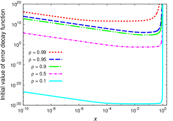
Figure 1: Impact of $\alpha$ ($=1+x(\rho^{-1}-1)$) on initial value $\,\widetilde{\!\widetilde{E}}{}_{N}(1)$

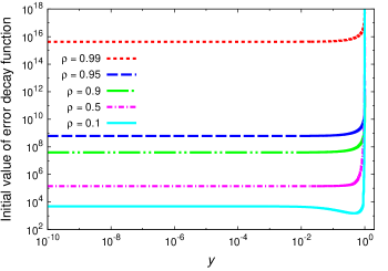
Figure 2: Impact of $\alpha^{\sharp}$ ($=\alpha+y(\rho^{-1}-\alpha)$) on initial value $\,\widetilde{\!\widetilde{E}}{}_{N}^{\sharp}(1)$

As expected, Figure 1 shows that $\,\widetilde{\!\widetilde{E}}{}_{N}(1)$ increases as $\alpha$ decreases toward one (i.e., $x$ decreases toward zero), and Figure 2 shows that $\,\widetilde{\!\widetilde{E}}{}_{N}^{\sharp}(1)$ increases as $\alpha^{\sharp}$ increases toward $\rho^{-1}$ (i.e., $y$ increases toward one). Furthermore, we can see from Figure 1 that $\,\widetilde{\!\widetilde{E}}{}_{N}(1)$ rapidly increases as $\alpha$ increases toward $\rho^{-1}$. This observation is justified as follows: It follows from (4.24) and (4.25) that if $\alpha\uparrow\rho^{-1}$ then $\gamma\downarrow\rho$ and thus $1/c\to\infty$. This result and (4.58) imply that $\,\widetilde{\!\widetilde{E}}{}_{N}(1)\to\infty$ as $\alpha\uparrow\rho^{-1}$.

It should be noted that $\alpha=1+10^{-3}$ in Figure 2, which corresponds to $x=10^{-3}/(\rho^{-1}-1)$ in Figure 1. Table 1 provides the values of $x$ for which $\alpha=1+10^{-3}$ in Figure 1.

Table 1: Values of $x$ for which $\alpha=1+10^{-3}$ in Figure 1

$\rho$	$x=\displaystyle{10^{-3}\over\rho^{-1}-1}$
0.1	$1.11\overline{1}\times 10^{-4}$
0.5	0.001
0.9	0.009
0.95	0.019
0.99	0.099

We can see from Figure 1 and Table 1 that $\,\widetilde{\!\widetilde{E}}{}_{N}(1)$ with $\alpha=1+10^{-3}$ takes a value not much different from the minimum for each $\rho=0.1,0.5,0.9,095,0.99$. In addition, $1+10^{-3}$ is close to one, i.e., the lower limit of $\alpha$. Recall here that the decay rate $\alpha^{\sharp}/\alpha$ of $\,\widetilde{\!\widetilde{E}}{}_{N}^{\sharp}$ is larger as $\alpha$ is smaller. Based on these facts, we set $\alpha=1+10^{-3}$ in the subsequent numerical examples.

According to (4.59), we can expect that the behavior of $\,\widetilde{\!\widetilde{E}}{}_{N}^{\sharp}$ is sensitive to the choice of $\alpha^{\sharp}$, provided that $\alpha$ is fixed. Thus, we observe the impact of $\alpha^{\sharp}$ on the error decay function $\,\widetilde{\!\widetilde{E}}{}_{N}^{\sharp}$. To this end, we define

$$\alpha_{i}=\alpha+{i\over 100}(\rho^{-1}-\alpha),\qquad i=0,1,10,50,90,99,$$

with $\alpha=1+10^{-3}$. We then denote by “line $i$” the $\,\widetilde{\!\widetilde{E}}{}_{N}(n)$’s with $\alpha=\alpha_{i}$ and denote by “line $(i,j)$” the $\,\widetilde{\!\widetilde{E}}{}_{N}^{\sharp}(n)$’s with $(\alpha,\alpha^{\sharp})=(\alpha_{i},\alpha_{j})$. Furthermore, we fix $\lambda=0.5s$ (thus $\rho=0.5$), $\beta=1$ and $N=K+100$. In this setting, Figure 3 plots

$$\mbox{lines $0,(0,1),(0,10),(0,50),(0,90),(0,99)$},$$

where line 0, i.e., the $\,\widetilde{\!\widetilde{E}}{}_{N}(n)$’s with $\alpha=1+10^{-3}$, serves as the “reference line” because the other lines must be over line 0 due to (4.62).

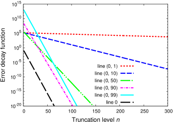
Figure 3: Impact of $\alpha^{\sharp}$ on $\,\widetilde{\!\widetilde{E}}{}_{N}^{\sharp}(n)$

As shown in Figure 3, the choice of large $\alpha^{\sharp}$ is basically better. Although the initial value of line $(0,99)$ is larger than that of line $(0,90)$, the decay rate of the former is larger than that of the latter and thus the two lines cross over eventually. Anyway, for later discussion, we fix $\alpha^{\sharp}=\alpha_{99}$.

Next, we discuss the impact of the traffic intensity $\rho$ on the decay rates of the error decay functions $\,\widetilde{\!\widetilde{E}}{}_{N}$ and $\,\widetilde{\!\widetilde{E}}{}_{N}^{\sharp}$. Inequality (4.63) shows that, as $\rho\uparrow 1$, the decay rate $\alpha^{\sharp}/\alpha$ of $\,\widetilde{\!\widetilde{E}}{}_{N}^{\sharp}$ becomes smaller and thus that of $\,\widetilde{\!\widetilde{E}}{}_{N}$ can be also smaller. In addition, (4.48) shows that if $\rho\uparrow 1$ then $\alpha\downarrow 1$, which leads to $\,\widetilde{\!\widetilde{E}}{}_{N}(1)\to\infty$ and $\,\widetilde{\!\widetilde{E}}{}_{N}^{\sharp}(1)\to\infty$ (see (4.64)). Consequently, as $\rho\uparrow 1$, the decay rates of $\,\widetilde{\!\widetilde{E}}{}_{N}$ and $\,\widetilde{\!\widetilde{E}}{}_{N}^{\sharp}$ decrease and their initial values $\,\widetilde{\!\widetilde{E}}{}_{N}(1)$ and $\,\widetilde{\!\widetilde{E}}{}_{N}^{\sharp}(1)$ increase, which is a “double whammy” for the bounds (4.46) and (4.57).

To visualize the impact of the traffic intensity $\rho$ on the error decay functions $\,\widetilde{\!\widetilde{E}}{}_{N}$ and $\,\widetilde{\!\widetilde{E}}{}_{N}^{\sharp}$, we provide Figures 4 and 5, where $s=\eta=50$, $\mu=1$, $\lambda=\rho s$, $\beta=1$ and $N=K+100$. Figures 4 and 5 plot lines 0 and (0,99), respectively, for $\rho=0.1,0.5,0.9,0.95,0.99$.

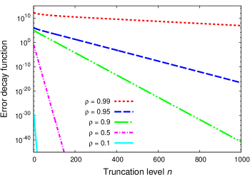
Figure 4: Impact of traffic intensity $\rho$ on $\,\widetilde{\!\widetilde{E}}{}_{N}(n)$ with $\alpha=\alpha_{0}$

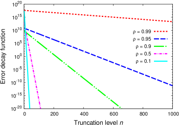
Figure 5: Impact of traffic intensity $\rho$ on $\,\widetilde{\!\widetilde{E}}{}_{N}^{\sharp}(n)$ with $(\alpha,\alpha^{\sharp})=(\alpha_{0},\alpha_{99})$

These two figures show that, in the case where $\rho=0.99$, the error decay functions $\,\widetilde{\!\widetilde{E}}{}_{N}$ and $\,\widetilde{\!\widetilde{E}}{}_{N}^{\sharp}$ take extremely large values and yield useless bounds in the region of the truncation level $n$ shown therein. This is mainly because the common factor $\overline{\phi}_{K,N}^{(\beta)}$ of $\,\widetilde{\!\widetilde{E}}{}_{N}$ and $\,\widetilde{\!\widetilde{E}}{}_{N}^{\sharp}$ (with $\beta=1$ in Figures 4 and 5) takes exceedingly small values, as shown in Table 2. Note here that Table 2 presents the values of $\overline{\phi}_{K,N}^{(1)}$ with $N=K+10,K+50,K+100,K+100,K+500$, which show the validity of our choice $N=K+100$ for computing $\overline{\phi}_{K,N}^{(\beta)}$.

Table 2: Values of $K$ and $\overline{\phi}_{K,N}^{(1)}$ in the same setting as Figures 4 and 5

		$\overline{\phi}_{K,N}^{(1)}$
$\rho$	$K$	$N=K+10$	$N=K+50$	$N=K+100$	$N=K+500$
0.1	1	$1.84\times 10^{-2}$	$1.84\times 10^{-2}$	$1.84\times 10^{-2}$	$1.84\times 10^{-2}$
0.5	2	$1.79\times 10^{-2}$	$1.79\times 10^{-2}$	$1.79\times 10^{-2}$	$1.79\times 10^{-2}$
0.9	18	$8.66\times 10^{-3}$	$8.66\times 10^{-3}$	$8.66\times 10^{-3}$	$8.66\times 10^{-3}$
0.95	38	$1.48\times 10^{-3}$	$1.52\times 10^{-3}$	$1.52\times 10^{-3}$	$1.52\times 10^{-3}$
0.99	219	$4.32\times 10^{-9}$	$4.52\times 10^{-9}$	$4.52\times 10^{-9}$	$4.52\times 10^{-9}$

We now discuss the impact of $\beta$ on the error decay functions $\,\widetilde{\!\widetilde{E}}{}_{N}$ and $\,\widetilde{\!\widetilde{E}}{}_{N}^{\sharp}$. It follows from (2.58) and (2.64) that if the minimum element of each column of $\bm{\Phi}_{\mathbb{F}_{N}}^{(\beta)}$ in (2.58) is small then so is $\overline{\phi}_{K,N}^{(\beta)}$. Since $\bm{Q}_{\mathbb{F}_{N}}$ considered here is block-tridiagonal, there can be a large variation in the elements of $\exp\{\bm{Q}_{\mathbb{F}_{N}}t\}$ for small values of $t$. However, such a variation would become smaller as $t$ increases, because $\bm{Q}_{\mathbb{F}_{N}}$ is irreducible. Furthermore, as $\beta$ is smaller, the integrand factor $\exp\{\bm{Q}_{\mathbb{F}_{N}}t\}$ for large values of $t$ (that is, the right tail of this factor) has a greater contribution to $\bm{\Phi}_{\mathbb{F}_{N}}^{(\beta)}$. Therefore, we can expect that $\overline{\phi}_{K,N}^{(\beta)}$ takes a large value if $\beta$ is small. In addition, it is known that the queue length process reaches the limiting state more slowly as $1-\rho$ approaches to zero (see, e.g., Doorn (2011); Kijima (1989, 1990)). As a result, it would be better to decrease $\beta$ with $1-\rho$ in order to keep the value of $\overline{\phi}_{K,N}^{(\beta)}$ “moderate”. Indeed, Table 4 shows that such choices of $\beta$ improve the values of $\overline{\phi}_{K,N}^{(\beta)}$ for $\rho=0.99$, compared to those of $\overline{\phi}_{K,N}^{(1)}$ in Table 2. Note here that Table 4 is provided in the same setting as Figures 4 and 5 except the value of $\beta$.

Table 3: Impact of $\beta$ on $\overline{\phi}_{K,N}^{(\beta)}$

	$\overline{\phi}_{K,N}^{(\beta)}$
$\rho$	$\beta=(1-\rho)^{1/2}$	$\beta=1-\rho$	$\beta=(1-\rho)^{2}$	$\beta=(1-\rho)^{3}$
0.1	$2.03\times 10^{-2}$	$2.23\times 10^{-2}$	$2.65\times 10^{-2}$	$3.09\times 10^{-2}$
0.5	$2.70\times 10^{-2}$	$3.65\times 10^{-2}$	$5.34\times 10^{-2}$	$6.50\times 10^{-2}$
0.9	$2.37\times 10^{-2}$	$3.70\times 10^{-2}$	$4.77\times 10^{-2}$	$4.92\times 10^{-2}$
0.95	$8.87\times 10^{-3}$	$2.10\times 10^{-2}$	$3.11\times 10^{-2}$	$2.13\times 10^{-2}$
0.99	$1.81\times 10^{-4}$	$2.11\times 10^{-3}$	$1.86\times 10^{-3}$	$2.67\times 10^{-5}$

Table 4: Impact of $\beta$ on $1/(\beta\overline{\phi}_{K,N}^{(\beta)})$

	$1/(\beta\overline{\phi}_{K,N}^{(\beta)})$
$\rho$	$\beta=(1-\rho)^{1/2}$	$\beta=1-\rho$	$\beta=(1-\rho)^{2}$	$\beta=(1-\rho)^{3}$
0.1	$5.20\times 10^{1}$	$4.99\times 10^{1}$	$4.66\times 10^{1}$	$4.44\times 10^{1}$
0.5	$5.24\times 10^{1}$	$5.48\times 10^{1}$	$7.49\times 10^{1}$	$1.23\times 10^{2}$
0.9	$1.34\times 10^{2}$	$2.70\times 10^{2}$	$2.10\times 10^{3}$	$2.03\times 10^{4}$
0.95	$5.04\times 10^{2}$	$9.53\times 10^{2}$	$1.29\times 10^{4}$	$3.76\times 10^{5}$
0.99	$5.52\times 10^{4}$	$4.74\times 10^{4}$	$5.39\times 10^{6}$	$3.74\times 10^{10}$

We have to remark that the error decay functions $\,\widetilde{\!\widetilde{E}}{}_{N}$ and $\,\widetilde{\!\widetilde{E}}{}_{N}^{\sharp}$ include a factor $1/(\beta\overline{\phi}_{K,N}^{(\beta)})$ and thus the small value of $\beta$ does not necessarily yield tight bounds, as shown in Table 4 provided in the same setting as Table 4. It would not be easy to systematically find an optimal value of $\beta$ such that $\,\widetilde{\!\widetilde{E}}{}_{N}$ and $\,\widetilde{\!\widetilde{E}}{}_{N}^{\sharp}$ are minimized. Anyway, we fix $\beta=1-\rho$ and present Figure 6, which plots the $\,\widetilde{\!\widetilde{E}}{}_{N}(n)$’s and the $\,\widetilde{\!\widetilde{E}}{}_{N}^{\sharp}(n)$’s in the same setting as Figures 4 and 5 except the value of $\beta$. Obviously, for sufficiently large $n$’s, $\,\widetilde{\!\widetilde{E}}{}_{N}(n)$ and $\,\widetilde{\!\widetilde{E}}{}_{N}^{\sharp}(n)$ are so small that the obtained bounds are practically useful even in the “worst” case, where $\rho=0.99$.

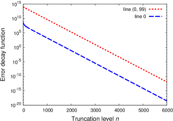
Figure 6: Values of $\,\widetilde{\!\widetilde{E}}{}_{N}(n)$ and $\,\widetilde{\!\widetilde{E}}{}_{N}^{\sharp}(n)$ with $\rho=0.99$ and $\beta=1-\rho$

5 Perturbation Bounds

In this section, we consider the perturbation bound for the stationary distribution vector $\bm{\pi}$ of $\bm{Q}$. Let $\bm{Q}^{\ast}=(q^{\ast}(k,i;\ell,j))_{(k,i;\ell,j)\in\mathbb{F}^{2}}$ denote the infinitesimal generator of an ergodic Markov chain with state space $\mathbb{F}$, and $\bm{\pi}^{\ast}=(\pi^{\ast}(k,i))_{(k,i)\in\mathbb{F}}$ denote the stationary distribution vector of $\bm{Q}^{\ast}$. Furthermore, we introduce the $\bm{v}$-norm $\|\,\cdot\,\|_{\bm{v}}$ for row vectors and matrices, where $\bm{v}=(v(k,i))_{(k,i)\in\mathbb{F}}$ is a nonnegative $|\mathbb{F}|\times 1$ vector, as in the previous sections. For any row vector $\bm{x}:=(x(k,i))_{(k,i)\in\mathbb{F}}$ and matrix $\bm{Z}:=(z(k,i;\ell,j))_{(k,i;\ell,j)\in\mathbb{F}^{2}}$, let $\|\bm{x}\|_{\bm{v}}$ and $\|\bm{Z}\|_{\bm{v}}$ denote

$$\|\bm{x}\|_{\bm{v}}=\sum_{(k,i)\in\mathbb{F}}|x(k,i)|\,v(k,i),\qquad\|\bm{Z}\|_{\bm{v}}=\sup_{(k,i)\in\mathbb{F}}{\sum_{(\ell,j)\in\mathbb{F}}|z(k,i;\ell,j)|\,v(\ell,j)\over v(k,i)},$$

respectively. By definition, $|\bm{x}|\,\bm{v}=\|\bm{x}\|_{\bm{v}}$.

We first present a perturbation bound under the exponential drift condition.

Theorem 5.1

Suppose that Assumption 2.1 is satisfied; and there exist some $b>0$, $c>0$, $K\in\mathbb{Z}_{+}$ and column vector $\bm{v}\geq\bm{e}/c$ such that (2.56) holds. Furthermore, fix $N\in\{K,K+1,\dots\}$ arbitrarily such that (2.61) holds; and suppose that

$$\|\bm{Q}^{\ast}-\bm{Q}\|_{\bm{v}}<{1\over C_{K,N}^{(\beta)}},$$ (5.1)

where

$$C_{K,N}^{(\beta)}={b+1\over c}\left(1+b+{2bc\over\beta\overline{\phi}_{K,N}^{(\beta)}}\right).$$ (5.2)

We then have

$$\|\bm{\pi}^{\ast}-\bm{\pi}\|_{\bm{v}} \leq {b\over c}\cdot{C_{K,N}^{(\beta)}\|\bm{Q}^{\ast}-\bm{Q}\|_{\bm{v}}\over 1-C_{K,N}^{(\beta)}\|\bm{Q}^{\ast}-\bm{Q}\|_{\bm{v}}}.$$ (5.3)

Remark 5.1

As mentioned in Section 2.2, we can compute $\overline{\phi}_{K,N}^{(\beta)}$ and thus $C_{K,N}^{(\beta)}$. Therefore, the perturbation bound (5.3) is computable, provided that $\|\bm{Q}^{\ast}-\bm{Q}\|_{\bm{v}}$ is obtained.

Remark 5.2

It follows from (2.65) and (5.2) that $\{C_{K,N}^{(\beta)};N=K,K+1,\dots\}$ is decreasing and

$$\lim_{N\to\infty}C_{K,N}^{(\beta)}={b+1\over c}\left(1+b+{2bc\over\beta\overline{\phi}_{K}^{(\beta)}}\right)=:C_{K}^{(\beta)}.$$

Thus, as $N$ increases, the bound (5.3) becomes tighter. In addition, if the conditions of Theorem 5.1 are satisfied and $\|\bm{Q}^{\ast}-\bm{Q}\|_{\bm{v}}<1/C_{K}^{(\beta)}$, then

$$\|\bm{\pi}^{\ast}-\bm{\pi}\|_{\bm{v}} \leq {b\over c}\cdot{C_{K}^{(\beta)}\|\bm{Q}^{\ast}-\bm{Q}\|_{\bm{v}}\over 1-C_{K}^{(\beta)}\|\bm{Q}^{\ast}-\bm{Q}\|_{\bm{v}}}.$$ (5.4)

Proof of Theorem 5.1.  Combining Lemma 2.3 with $\bm{f}=c\bm{v}\geq\bm{e}$ and $\bm{\pi}\bm{v}<b/c$ yields

$$|\bm{D}|\,\bm{v} \leq {c\bm{\pi}\bm{v}+1\over c}\left[\bm{v}+\left(\bm{\pi}\bm{v}+{2b\over\beta\overline{\phi}_{K}^{(\beta)}}\right)(c\bm{v})\right]\leq{b+1\over c}\left(1+b+{2bc\over\beta\overline{\phi}_{K}^{(\beta)}}\right)\bm{v}.$$

Furthermore, applying (2.65) to the above inequality leads to

$$|\bm{D}|\,\bm{v} \leq {b+1\over c}\left(1+b+{2bc\over\beta\overline{\phi}_{K,N}^{(\beta)}}\right)\bm{v}=C_{K,N}^{(\beta)}\bm{v},$$

which implies that

$$\|\bm{D}\|_{\bm{v}}\leq C_{K,N}^{(\beta)}.$$ (5.5)

From (5.1) and (5.5), we have

$$\|(\bm{Q}^{\ast}-\bm{Q})\bm{D}\|_{\bm{v}}\leq\|(\bm{Q}^{\ast}-\bm{Q})\|_{\bm{v}}\cdot\|\bm{D}\|_{\bm{v}}\leq C_{K,N}^{(\beta)}\|(\bm{Q}^{\ast}-\bm{Q})\|_{\bm{v}}<1.$$

Thus, it holds (see, e.g., Heidergott et al. (2010, Section 4.1)) that

$$\bm{\pi}^{\ast}-\bm{\pi} = \bm{\pi}\sum_{m=1}^{\infty}\{(\bm{Q}^{\ast}-\bm{Q})\bm{D}\}^{m}.$$ (5.6)

It follows from (5.5) and (5.6) that

$$\|\bm{\pi}^{\ast}-\bm{\pi}\|_{\bm{v}} \leq \|\bm{\pi}\|_{\bm{v}}\sum_{m=1}^{\infty}\left\{\|\bm{Q}^{\ast}-\bm{Q}\|_{\bm{v}}\cdot\|\bm{D}\|_{\bm{v}}\right\}^{m}$$

$$\leq \|\bm{\pi}\|_{\bm{v}}\sum_{m=1}^{\infty}\left\{C_{K,N}^{(\beta)}\|\bm{Q}^{\ast}-\bm{Q}\|_{\bm{v}}\right\}^{m}$$

$$\leq {b\over c}\cdot{C_{K,N}^{(\beta)}\|\bm{Q}^{\ast}-\bm{Q}\|_{\bm{v}}\over 1-C_{K,N}^{(\beta)}\|\bm{Q}^{\ast}-\bm{Q}\|_{\bm{v}}},$$

where the last inequality holds because $\|\bm{\pi}\|_{\bm{v}}=\bm{\pi}\bm{v}\leq b/c$. $\Box$

Remark 5.3

Kartashov (1986a, b, c) considered discrete-time infinite-state Markov chains with uniform ergodicity (or equivalently, strong stability; see Kartashov (1986a, Theorem B)), and then derived perturbation bounds of a type similar to the bound (5.3):

$$\|\bm{\varpi}^{\ast}-\bm{\varpi}\|\leq C_{1}\cdot{C_{2}\|\bm{P}^{\ast}-\bm{P}\|\over 1-C_{2}\|\bm{P}^{\ast}-\bm{P}\|},$$ (5.7)

where $\|\cdot\|$ denotes an appropriate norm, and where $\bm{\varpi}$ and $\bm{\varpi}^{\ast}$ are the stationary distributions of the original transition kernel $\bm{P}$ and a perturbated transition kernel $\bm{P}^{\ast}$, respectively. Mouhoubi and Aïssani (2010) established a bound of the type (5.7) by using the norm of a residual matrix of the original transition probability matrix (see Theorem 5 therein). However, the perturbation bounds in these previous studies are not easy to compute because the parameters $C_{1}$ and $C_{2}$ depend on $\|\bm{\varpi}\|$. As for continuous-time infinite-state Markov chains, Liu (2012) presented a perturbation bound that is similar to the bound (5.3) and independent of $\|\bm{\pi}\|_{\bm{v}}$, under such an exponential drift condition as corresponds to the condition (2.56) with $\bm{1}_{\mathbb{F}_{K}}$ being replaced by $\bm{1}_{\{(k,i)\}}$, together with the condition that the infinitesimal generator is bounded. The boundedness of the infinitesimal generator is removed by Liu (2015).

Next we derive a perturbation bound under the general $\bm{f}$-modulated drift condition. To this end, we use the reduction to exponential ergodicity, as in Theorem 3.1. Recall here that if Condition 1.1 holds then $\widehat{\bm{Q}}=\bm{\Delta}_{\bm{v}/\bm{f}}\bm{Q}$ satisfies the exponential drift condition (3.8), which leads to (3.9). Note also that, for all sufficiently large $N\in\{K,K+1,\dots\}$,

$$\left[\widehat{\bm{\Phi}}_{\mathbb{F}_{N}}^{(\beta)}\right]_{\mathbb{F}_{K}}>\bm{O},$$ (5.8)

which is confirmed as in the argument leading to (2.61). We now fix $N\in\{K,K+1,\dots\}$ such that (5.8) holds. We then define $\widehat{\bm{\Phi}}_{\mathbb{F}_{N}}^{(\beta)}:=(\widehat{\phi}_{\mathbb{F}_{N}}^{(\beta)}(k,i;\ell,j))_{(k,i;\ell,j)\in\mathbb{F}^{2}}$ as

$$\widehat{\bm{\Phi}}_{\mathbb{F}_{N}}^{(\beta)}=(\bm{I}-\widehat{\bm{Q}}_{\mathbb{F}_{N}}/\beta)^{-1},$$

where $\widehat{\bm{Q}}_{\mathbb{F}_{N}}=\bm{\Delta}_{\bm{v}/\bm{f}}\bm{Q}_{\mathbb{F}_{N}}$. We also define $\widehat{C}_{K,N}^{(\beta)}$ as

$$\widehat{C}_{K,N}^{(\beta)}=(\widehat{b}+1)\left(1+\widehat{b}+{2\widehat{b}\over\beta\overline{\widehat{\phi}\,}{}_{K,N}^{(\beta)}}\right),$$ (5.9)

where

$$\overline{\widehat{\phi}\,}{}_{K,N}^{(\beta)}=\sup_{(\ell,j)\in\mathbb{F}_{N}}\min_{(k,i)\in\mathbb{F}_{K}}\widehat{\phi}_{\mathbb{F}_{N}}^{(\beta)}(k,i;\ell,j)>0.$$

Since $\overline{\widehat{\phi}\,}{}_{K,N}^{(\beta)}$ corresponds to $\overline{\phi}_{K,N}^{(\beta)}$ in (2.64), the former can be computed in a similar way to the computation of the latter (see Remark 2.6).

The following theorem presents a computable perturbation bound under the general $\bm{f}$-modulated drift condition.

Theorem 5.2

Suppose that Assumption 2.1 and Condition 3.1 are satisfied. Furthermore, fix $N\in\{K,K+1,\dots\}$ arbitrarily such that (5.8) holds. If $\bm{\pi}\bm{v}<\infty$ and

$$\|\bm{\Delta}_{\bm{v}/\bm{f}}(\bm{Q}^{\ast}-\bm{Q})\|_{\bm{v}} < {1\over\widehat{C}_{K,N}^{(\beta)}},$$ (5.10)

then

$$\|\bm{\pi}^{\ast}-\bm{\pi}\|_{\bm{f}} \leq \overline{C}{}_{\bm{f}/\bm{v}}\left(1+\widehat{b}\,\overline{C}{}_{\bm{f}/\bm{v}}\right)\cdot{\widehat{b}\widehat{C}_{K,N}^{(\beta)}\|\bm{\Delta}_{\bm{v}/\bm{f}}(\bm{Q}^{\ast}-\bm{Q})\|_{\bm{v}}\over 1-\widehat{C}_{K,N}^{(\beta)}\|\bm{\Delta}_{\bm{v}/\bm{f}}(\bm{Q}^{\ast}-\bm{Q})\|_{\bm{v}}}.$$ (5.11)

Proof.  Let $\widehat{\bm{\pi}}^{\ast}$ and $\widehat{\bm{Q}}^{\ast}$ denote

$$\widehat{\bm{\pi}}^{\ast}={\bm{\pi}^{\ast}\bm{\Delta}_{\bm{f}/\bm{v}}\over\bm{\pi}^{\ast}(\bm{f}/\bm{v})},\qquad\widehat{\bm{Q}}^{\ast}=\bm{\Delta}_{\bm{v}/\bm{f}}\bm{Q}^{\ast},$$

respectively, where $\widehat{\bm{\pi}}^{\ast}$ is the probability vector such that $\widehat{\bm{\pi}}^{\ast}\widehat{\bm{Q}}^{\ast}=\bm{0}$. Proceeding as in the derivation of (3.15), we have

$$\bm{\pi}^{\ast}-\bm{\pi}={1\over\widehat{\bm{\pi}}^{\ast}\left(\bm{v}/\bm{f}\right)}\left[(\widehat{\bm{\pi}}^{\ast}-\widehat{\bm{\pi}})+(\widehat{\bm{\pi}}-\widehat{\bm{\pi}}^{\ast})\left(\bm{v}/\bm{f}\right){\widehat{\bm{\pi}}\over\widehat{\bm{\pi}}\left(\bm{v}/\bm{f}\right)}\right]\bm{\Delta}_{\bm{v}/\bm{f}}.$$

Using this equation and (3.21), we obtain

$$\|\bm{\pi}^{\ast}-\bm{\pi}\|_{\bm{f}} \leq {1\over\widehat{\bm{\pi}}^{\ast}\left(\bm{v}/\bm{f}\right)}\left[|\widehat{\bm{\pi}}^{\ast}-\widehat{\bm{\pi}}|+|\widehat{\bm{\pi}}-\widehat{\bm{\pi}}^{\ast}|\left(\bm{v}/\bm{f}\right){\widehat{\bm{\pi}}\over\widehat{\bm{\pi}}\left(\bm{v}/\bm{f}\right)}\right]\bm{v}$$ (5.12)

$$\leq {1\over\widehat{\bm{\pi}}^{\ast}\left(\bm{v}/\bm{f}\right)}\left[|\widehat{\bm{\pi}}^{\ast}-\widehat{\bm{\pi}}|\bm{v}+|\widehat{\bm{\pi}}-\widehat{\bm{\pi}}^{\ast}|\bm{v}\cdot{\widehat{\bm{\pi}}\bm{v}\over\widehat{\bm{\pi}}\left(\bm{v}/\bm{f}\right)}\right]$$

$$= {1\over\widehat{\bm{\pi}}^{\ast}\left(\bm{v}/\bm{f}\right)}\left(1+{\widehat{\bm{\pi}}\bm{v}\over\widehat{\bm{\pi}}\left(\bm{v}/\bm{f}\right)}\right)\|\widehat{\bm{\pi}}^{\ast}-\widehat{\bm{\pi}}\|_{\bm{v}}$$

$$\leq \overline{C}_{\bm{f}/\bm{v}}\left(1+\widehat{\bm{\pi}}\bm{v}\cdot\overline{C}_{\bm{f}/\bm{v}}\right)\|\widehat{\bm{\pi}}^{\ast}-\widehat{\bm{\pi}}\|_{\bm{v}}$$

$$\leq \overline{C}_{\bm{f}/\bm{v}}\left(1+\widehat{b}\,\overline{C}_{\bm{f}/\bm{v}}\right)\|\widehat{\bm{\pi}}^{\ast}-\widehat{\bm{\pi}}\|_{\bm{v}},$$

where the last inequality follows from (3.9).

It remains to estimate $\|\widehat{\bm{\pi}}^{\ast}-\widehat{\bm{\pi}}\|_{\bm{v}}$. From (5.10), $\widehat{\bm{Q}}=\bm{\Delta}_{\bm{v}/\bm{f}}\bm{Q}$ and $\widehat{\bm{Q}}^{\ast}=\bm{\Delta}_{\bm{v}/\bm{f}}\bm{Q}^{\ast}$, we have

$$\|\widehat{\bm{Q}}^{\ast}-\widehat{\bm{Q}}\|_{\bm{v}}=\|\bm{\Delta}_{\bm{v}/\bm{f}}(\bm{Q}^{\ast}-\bm{Q})\|_{\bm{v}}<{1\over\widehat{C}_{K,N}^{(\beta)}}.$$

Thus, applying Theorem 5.1 to $\widehat{\bm{Q}}$ satisfying (3.8), we obtain

$$\left\|\widehat{\bm{\pi}}^{\ast}-\widehat{\bm{\pi}}\right\|_{\bm{v}}\leq\widehat{b}{\widehat{C}_{K,N}^{(\beta)}\|\widehat{\bm{Q}}^{\ast}-\widehat{\bm{Q}}\|_{\bm{v}}\over 1-\widehat{C}_{K,N}^{(\beta)}\|\widehat{\bm{Q}}^{\ast}-\widehat{\bm{Q}}\|_{\bm{v}}}={\widehat{b}\,\widehat{C}_{K,N}^{(\beta)}\|\bm{\Delta}_{\bm{v}/\bm{f}}(\bm{Q}^{\ast}-\bm{Q})\|_{\bm{v}}\over 1-\widehat{C}_{K,N}^{(\beta)}\|\bm{\Delta}_{\bm{v}/\bm{f}}(\bm{Q}^{\ast}-\bm{Q})\|_{\bm{v}}}.$$ (5.13)

Substituting (5.13) into (5.12) results in (5.11). $\Box$

Remark 5.4

A similar remark to Remark 5.2 applies to the bound (5.11). To save space, we omit the details.

Appendix A Proof of Proposition 1.1

We first prove statement (i). From (1.3), we have

$$\hskip 0.50003pt{}_{(n)}q(k,i;\ell,j)=0,\qquad(k,i)\in\mathbb{F}_{n},\ (\ell,j)\in\overline{\mathbb{F}}_{n},$$

which shows that the Markov chain $\{(\hskip 0.50003pt{}_{(n)}X(t),\hskip 0.50003pt{}_{(n)}J(t))\}$ cannot move from $\mathbb{F}_{n}$ to $\overline{\mathbb{F}}_{n}$. Thus, $\mathbb{F}_{n}$ is closed and therefore includes at least one closed communicating class.

We now denote by $\mathbb{C}$ a closed communicating class in $\mathbb{F}_{n}$. We then assume that $\mathbb{C}\cap\mathbb{L}_{n}=\emptyset$, i.e., $\mathbb{C}\subseteq\mathbb{F}_{n-1}$. In this setting, the submatrix $\hskip 0.50003pt{}_{(n)}\bm{Q}_{\mathbb{C}}:=(\hskip 0.50003pt{}_{(n)}q(k,i;\ell,j))_{(k,i;\ell,j)\in\mathbb{C}^{2}}$ of $\hskip 0.50003pt{}_{(n)}\bm{Q}$ is a conservative $q$-matrix. Furthermore, it follows from (1.3) and $\mathbb{C}\subseteq\mathbb{F}_{n-1}$ that $\hskip 0.50003pt{}_{(n)}\bm{Q}_{\mathbb{C}}$ is equal to the submatrix $\bm{Q}_{\mathbb{C}}:=(q(k,i;\ell,j))_{(k,i;\ell,j)\in\mathbb{C}^{2}}$ of the original generator $\bm{Q}$, i.e., $\hskip 0.50003pt{}_{(n)}\bm{Q}_{\mathbb{C}}=\bm{Q}_{\mathbb{C}}$. Therefore, $\bm{Q}_{\mathbb{C}}$ is a conservative $q$-matrix, and $\mathbb{C}$ is a closed communicating class in the original Markov chain $\{(X(t),J(t))\}$ with infinitesimal generator $\bm{Q}$. This is, however, inconsistent with the irreducibility of the Markov chain $\{(X(t),J(t))\}$. As a result, $\mathbb{C}\cap\mathbb{L}_{n}\neq\emptyset$.

According to the above discussion, any closed communicating class in $\mathbb{F}_{n}$ shares at least one element with $\mathbb{L}_{n}$. This implies that the number of closed communicating classes in $\mathbb{F}_{n}$ is not greater than the cardinality of $\mathbb{L}_{n}$, i.e., $S_{1}+1$. Consequently, statement (i) has been proved.

Next we prove statement (ii). To this end, we assume that there exists a closed communicating class $\mathbb{C}$ in $\overline{\mathbb{F}}_{n}$. Recall here that the $|\overline{\mathbb{F}}_{n}|\times|\overline{\mathbb{F}}_{n}|$ southeast corner of $\hskip 0.50003pt{}_{(n)}\bm{Q}$ is block-diagonal due to (1.3). Thus, the closed communicating class $\mathbb{C}$ is within a single level, i.e., $\mathbb{C}\subseteq\mathbb{L}_{k}$ for some $k\geq n+1$, which implies that the $|\mathbb{C}|\times|\mathbb{C}|$ submatrix of $\hskip 0.50003pt{}_{(n)}\bm{Q}(k;k)=\bm{Q}(k;k)$ is a conservative $q$-matrix. Therefore, the original Markov chain $\{(X(t),J(t))\}$ with infinitesimal generator $\bm{Q}$ cannot move out of $\mathbb{C}\subseteq\mathbb{L}_{k}$. This contradicts the irreducibility of the Markov chain $\{(X(t),J(t))\}$. Therefore, there are no closed communicating classes in $\overline{\mathbb{F}}_{n}$.

Appendix B Applications of Dynkin’s Formula

In this appendix, we present two applications of Dynkin’s formula (see, e.g., Meyn and Tweedie (1993b)). For convenience, we redefine some of the symbols used in the body of the paper, in a different way.

We define $\{Y(t);t\geq 0\}$ as an irreducible regular-jump Markov chain with state space $\mathbb{Z}_{+}$ and infinitesimal generator $\bm{Q}:=(q(i,j))_{i,j\in\mathbb{Z}_{+}}$. For any $m\in\mathbb{N}$, we also define $\{Y_{m}(t);t\geq 0\}$ as a stochastic process such that

$$Y_{m}(t)=\left\{\begin{array}[]{ll}Y(t),&t<\tau_{m},\\ Y(\tau_{m}),&t\geq\tau_{m},\end{array}\right.$$ (B.1)

where $\tau_{m}=\inf\{t\geq 0:Y(t)\geq m\}$. Since $\tau_{m}$ is a stopping time for the Markov chain $\{Y(t)\}$, the stochastic process $\{Y_{m}(t)\}$ is also a Markov chain (see, e.g., Brémaud (1999, Chapter 8, Theorem 4.1)).

For any $m\in\mathbb{N}$, let $\bm{Q}_{m}:=(q_{m}(i,j))_{i,j\in\mathbb{Z}_{+}}$ denote the infinitesimal generator of $\{Y_{m}(t)\}$. It then follows from (B.1) that

$$q_{m}(i,j)=\left\{\begin{array}[]{lll}q(i,j),&i=0,1,\dots,m-1,&j\in\mathbb{Z}_{+},\\ 0,&i=m,m+1,\dots,&j\in\mathbb{Z}_{+}.\end{array}\right.$$ (B.2)

Furthermore, since $\{Y(t)\}$ is non-explosive, so is $\{Y_{m}(t)\}$ and thus

$$\mathsf{P}_{i}\!\left(\lim_{m\to\infty}\tau_{m}=\infty\right)=1\quad\mbox{for all~{}}i\in\mathbb{Z}_{+},$$ (B.3)

where $\mathsf{P}_{i}(\,\,\cdot\,\,)$ represents $\mathsf{P}(~{}\cdot\mid Y(0)=i)$ or $\mathsf{P}(~{}\cdot\mid Y_{m}(0)=i)$. For later use, let $\mathsf{E}_{i}[\,\,\cdot\,\,]$ denote $\mathsf{E}[~{}\cdot\mid Y(0)=i]$ or $\mathsf{E}[~{}\cdot\mid Y_{m}(0)=i]$.

Let $\widehat{\tau}_{m}=\min(m,\tau_{m},\tau)$ for $m\in\mathbb{N}$, where $\tau$ denotes an arbitrary stopping time for the Markov chain $\{Y(t)\}$. It then follows from (B.1) and Dynkin’s formula (see, e.g., Meyn and Tweedie (1993b, Equation (8))) that, for any real-valued column vector $\bm{x}:=(x(i))_{i\in\mathbb{Z}_{+}}$,

$$\mathsf{E}_{i}\!\left[x(Y(\widehat{\tau}_{m}))\right] = \mathsf{E}_{i}\!\left[x(Y_{m}(\widehat{\tau}_{m}))\right]$$ (B.4)

$$= x(i)+\mathsf{E}_{i}\!\!\left[\int_{0}^{\widehat{\tau}_{m}}(\bm{Q}_{m}\bm{x})(Y(u)){\rm d}u\right],\qquad i=0,1,\dots,m-1,$$

where $(\bm{Q}_{m}\bm{x})(i)$ is the $i$th element of the vector $\bm{Q}_{m}\bm{x}$. Using (B.4), we obtain Lemma B.1 below, which is a continuous analogue of the comparison Theorem for discrete-time Markov chains (see Glynn and Meyn (1996, Theorem 2.1)).

Lemma B.1

Suppose that $\{Y(t);t\geq 0\}$ is an irreducible regular-jump Markov chain. If there exist nonnegative column vectors $\bm{v}:=(v(i))_{i\in\mathbb{Z}_{+}}$, $\bm{f}:=(f(i))_{i\in\mathbb{Z}_{+}}$ and $\bm{w}:=(w(i))_{i\in\mathbb{Z}_{+}}$ such that

$$\bm{Q}\bm{v}\leq-\bm{f}+\bm{w},$$ (B.5)

then, for any $t\geq 0$ and stopping time $\tau$,

$$\mathsf{E}_{i}\!\!\left[\int_{0}^{t}f(Y(u)){\rm d}u\right] \leq v(i)+\mathsf{E}_{i}\!\!\left[\int_{0}^{t}w(Y(u)){\rm d}u\right], i\in\mathbb{Z}_{+},$$ (B.6)

$$\mathsf{E}_{i}\!\!\left[\int_{0}^{\tau}f(Y(u)){\rm d}u\right] \leq v(i)+\mathsf{E}_{i}\!\!\left[\int_{0}^{\tau}w(Y(u)){\rm d}u\right], i\in\mathbb{Z}_{+}.$$ (B.7)

Proof.  It follows from (B.2) and (B.5) that, for $m\in\mathbb{N}$,

$$(\bm{Q}_{m}\bm{v})(i) \leq-f(i)+w(i), i =0,1,\dots,m-1,$$ (B.8)

$$(\bm{Q}_{m}\bm{v})(i) =0, i =m,m+1,\dots.$$ (B.9)

Substituting (B.8) and (B.9) into (B.4) with $\bm{x}=\bm{v}$ yields

$$0 \leq \mathsf{E}_{i}\!\left[v(Y(\widehat{\tau}_{m}))\right]$$ (B.10)

$$\leq v(i)+\mathsf{E}_{i}\!\!\left[\int_{0}^{\widehat{\tau}_{m}}w(Y(u)){\rm d}u\right]-\mathsf{E}_{i}\!\!\left[\int_{0}^{\widehat{\tau}_{m}}f_{m}(Y(u)){\rm d}u\right],\qquad i\in\mathbb{Z}_{+},$$

where

$$f_{m}(i)=\left\{\begin{array}[]{ll}f(i),&i=0,1,\dots,m-1,\\ f(i)\wedge w(i),&i=m,m+1,\dots.\end{array}\right.$$

Adding $\mathsf{E}_{i}[\int_{0}^{\widehat{\tau}_{m}}f_{m}(Y(u)){\rm d}u]$ to both sides of (B.10), we obtain

$$\mathsf{E}_{i}\!\!\left[\int_{0}^{\widehat{\tau}_{m}}f_{m}(Y(u)){\rm d}u\right] \leq v(i)+\mathsf{E}_{i}\!\!\left[\int_{0}^{\widehat{\tau}_{m}}w(Y(u)){\rm d}u\right]$$ (B.11)

$$\leq v(i)+\mathsf{E}_{i}\!\!\left[\int_{0}^{\tau}w(Y(u)){\rm d}u\right],\qquad i\in\mathbb{Z}_{+},$$

where the second inequality follows from $\widehat{\tau}_{m}=\min(m,\tau_{m},\tau)\leq\tau$. Note here that (B.3) yields $\mathsf{P}_{i}(\lim_{m\to\infty}m\wedge\tau_{m}=\infty)=1$ and thus $\mathsf{P}_{i}(\lim_{m\to\infty}\widehat{\tau}_{m}=\tau)=1$. Therefore, letting $m\to\infty$ in (B.11) and using the monotone convergence theorem, we have (B.7). Furthermore, replacing $\tau$ by $t$ and proceeding as in the derivation of (B.11), we obtain

$$\mathsf{E}_{i}\!\!\left[\int_{0}^{t\wedge(m\wedge\tau_{m})}f_{m}(Y(u)){\rm d}u\right]\leq v(i)+\mathsf{E}_{i}\!\!\left[\int_{0}^{t}w(Y(u)){\rm d}u\right],\qquad i\in\mathbb{Z}_{+}.$$

Letting $m\to\infty$ in the above inequality, we have (B.6). $\Box$

Next we discuss a Poisson equation associated with $\bm{Q}$. To this end, we assume that the Markov chain $\{Y(t)\}$ is ergodic and has the unique stationary distribution vector $\bm{\pi}:=(\pi(i))_{i\in\mathbb{Z}_{+}}$. We then define $\bm{g}^{{\ddagger}}:=(g^{{\ddagger}}(i))_{i\in\mathbb{Z}_{+}}$ as $\bm{g}^{{\ddagger}}=\bm{g}-(\bm{\pi}\bm{g})\bm{e}$, i.e.,

$$g^{{\ddagger}}(i)=g(i)-\bm{\pi}\bm{g},\qquad i\in\mathbb{Z}_{+},$$

where $\bm{g}:=(g(i))_{i\in\mathbb{Z}_{+}}$ is a given real-valued column vector. In this setting, we consider a Poisson equation:

$$-\bm{Q}\bm{h}=\bm{g}^{{\ddagger}}.$$ (B.12)

Using Lemma B.1, we prove the following result on a solution of (B.12).

Lemma B.2

Suppose that $\{Y(t);t\geq 0\}$ is an irreducible regular-jump Markov chain, and there exist some $b>0$, $K\in\mathbb{Z}_{+}$, column vectors $\bm{v}\geq\bm{0}$ and $\bm{f}\geq\bm{e}$ such that

$$\bm{Q}\bm{v}\leq-\bm{f}+b\bm{1}_{\mathbb{F}_{K}}.$$

For any fixed $j_{\ast}\in\mathbb{Z}_{+}$ and $|\bm{g}|\leq\bm{f}$, let $\bm{h}_{j_{\ast}}:=(h_{j_{\ast}}(i))_{i\in\mathbb{Z}_{+}}$ denote

$$h_{j_{\ast}}(i)=\mathsf{E}_{i}\!\!\left[\int_{0}^{\tau(j_{\ast})}g^{{\ddagger}}(Y(t)){\rm d}t\right],\qquad i\in\mathbb{Z}_{+},$$ (B.13)

where $\tau(j_{\ast})=\inf\{t\geq 0:Y(t)=j_{\ast}\}$. Under these conditions, the vector $\bm{h}_{j_{\ast}}$ is a solution of the Poisson equation (B.12). In addition, $h_{j_{\ast}}(j_{\ast})=0$.

Proof.  According to Theorem 7 of Meyn and Tweedie (1993a), the Markov chain $\{Y(t)\}$ is ergodic under the conditions of this lemma. It follows from Lemma B.1 with $\tau=\tau(j_{\ast})$ and $\bm{w}=\bm{1}_{\mathbb{F}_{K}}$ that

$$\mathsf{E}_{i}\!\!\left[\int_{0}^{\tau(j_{\ast})}|g(Y(u))|{\rm d}u\right] \leq \mathsf{E}_{i}\!\!\left[\int_{0}^{\tau(j_{\ast})}f(Y(u)){\rm d}u\right]$$

$$\leq v(i)+\mathsf{E}_{i}\!\!\left[\int_{0}^{\tau(j_{\ast})}1_{\mathbb{F}_{K}}(Y(u)){\rm d}u\right]$$

$$\leq v(i)+\mathsf{E}_{i}[\tau(j_{\ast})]<\infty,\qquad i,j\in\mathbb{Z}_{+},$$

where the last inequality is due to the ergodicity of the Markov chain $\{Y(t)\}$. Therefore, $\bm{h}_{j_{\ast}}$ is well-defined. Furthermore, given $Y(0)=j_{\ast}$, we have $\tau(j_{\ast})=0$ and thus $h_{j_{\ast}}(j_{\ast})=0$.

In what follows, we confirm that $\bm{h}_{j_{\ast}}$ is a solution of (B.12). For this purpose, we consider the embedded Markov chain $\{\widetilde{Y}_{n}:=Y(t_{n});n\in\mathbb{Z}_{+}\}$ of the Markov chain $\{Y(t);t\geq 0\}$ (see, e.g., Brémaud (1999, Chapter 8, Section 4.2)), where $\{t_{n};n\in\mathbb{Z}_{+}\}$ denotes a sequence of time points such that $t_{0}=0$ and

$$t_{n}=\inf\{t>t_{n-1}:Y(t)\neq Y(t_{n-1})\},\qquad n\in\mathbb{N}.$$

The transition probability matrix of $\{\widetilde{Y}_{n}\}$, denoted by $\widetilde{\bm{P}}:=(\widetilde{p}(i,j))_{i,j\in\mathbb{Z}_{+}}$, is given by

$$\widetilde{p}(i,j)=\left\{\begin{array}[]{cc}0,&j=i,\\ \displaystyle{q(i,j)\over|q(i,i)|},&j\neq i.\end{array}\right.$$ (B.14)

We also define $\widetilde{\tau}(j)=\inf\{n\in\mathbb{Z}_{+}:\widetilde{Y}_{n}=j\}$ for $j\in\mathbb{Z}_{+}$ and $\Delta t_{n}=t_{n}-t_{n-1}$ for $n\in\mathbb{N}$. It then follows from (B.13) that

$$h_{j_{\ast}}(i) = \mathsf{E}_{i}\!\!\left[\sum_{n=0}^{\widetilde{\tau}(j_{\ast})-1}\Delta t_{n+1}g^{{\ddagger}}(\widetilde{Y}_{n})\right]$$ (B.15)

$$= \sum_{n=0}^{\infty}\mathsf{E}_{i}[\Delta t_{n+1}g^{{\ddagger}}(\widetilde{Y}_{n})I(n<\widetilde{\tau}(j_{\ast}))]$$

$$= \sum_{n=0}^{\infty}\sum_{\nu\in\mathbb{Z}_{+}}g^{{\ddagger}}(\nu)\mathsf{E}_{i}[\Delta t_{n+1}I(n<\widetilde{\tau}(j_{\ast}))I(\widetilde{Y}_{n}=\nu)]$$

$$= \sum_{n=0}^{\infty}\sum_{\nu\in\mathbb{Z}_{+}}g^{{\ddagger}}(\nu)\mathsf{E}_{i}[\Delta t_{n+1}\mid n<\widetilde{\tau}(j_{\ast}),\widetilde{Y}_{n}=\nu]\cdot\mathsf{E}_{i}[I(n<\widetilde{\tau}(j_{\ast}))I(\widetilde{Y}_{n}=\nu)],\qquad$$

where $I(\,\cdot\,)$ denotes the indicator function of the event in the brackets. Since $\widetilde{\tau}(j_{\ast})$ is a stopping time for $\{\widetilde{Y}_{n}\}$, the event $\{n<\widetilde{\tau}(j_{\ast})\}$ is determined by the set $\{\widetilde{Y}_{m};m=0,1,\dots,m\}=\{Y(t_{m});m=0,1,\dots,m\}$. Thus, given that $\widetilde{Y}_{n}=Y(t_{n})=\nu$, the random variable $\Delta t_{n+1}=t_{n+1}-t_{n}$ is independent of the event $\{n<\widetilde{\tau}(j_{\ast})\}$, which leads to

$$\mathsf{E}_{i}[\Delta t_{n+1}\mid n<\widetilde{\tau}(j_{\ast}),\widetilde{Y}_{n}=\nu]=\mathsf{E}[\Delta t_{n+1}\mid\widetilde{Y}_{n}=\nu]={1\over|q(\nu,\nu)|},\qquad\nu\in\mathbb{Z}_{+}.$$ (B.16)

Substituting (B.16) into (B.15) yields

$$h_{j_{\ast}}(i) = \sum_{n=0}^{\infty}\sum_{\nu\in\mathbb{Z}_{+}}{g^{{\ddagger}}(\nu)\over|q(\nu,\nu)|}\mathsf{E}_{i}[I(n<\widetilde{\tau}(j_{\ast}))I(\widetilde{Y}_{n}=\nu)]$$ (B.17)

$$= \mathsf{E}_{i}\!\!\left[\sum_{n=0}^{\widetilde{\tau}(j_{\ast})-1}\sum_{\nu\in\mathbb{Z}_{+}}{g^{{\ddagger}}(\nu)\over|q(\nu,\nu)|}I(\widetilde{Y}_{n}=\nu)\right]=\mathsf{E}_{i}\!\!\left[\sum_{n=0}^{\widetilde{\tau}(j_{\ast})-1}\widetilde{g}(\widetilde{Y}_{n})\right],$$

where $\widetilde{g}(\nu)=g^{{\ddagger}}(\nu)/|q(\nu,\nu)|$ for $\nu\in\mathbb{Z}_{+}$. From (B.17), $\widetilde{p}(i,i)=0$ and the Markov property of $\{\widetilde{Y}_{n}\}$, we have

$$h_{j_{\ast}}(i) = \widetilde{g}(i)+\mathsf{E}_{i}\!\!\left[\sum_{n=1}^{\widetilde{\tau}(j_{\ast})-1}\widetilde{g}(\widetilde{Y}_{n})\cdot I(\widetilde{\tau}(j_{\ast})\geq 2)\right]$$ (B.18)

$$= \widetilde{g}(i)+\sum_{\nu\in\mathbb{Z}_{+}\setminus\{i,j_{\ast}\}}\widetilde{p}(i,\nu)\mathsf{E}\!\!\left[\sum_{n=1}^{\widetilde{\tau}(j_{\ast})-1}\widetilde{g}(\widetilde{Y}_{n})\cdot I(\widetilde{\tau}(j_{\ast})\geq 2)\mid\widetilde{Y}_{1}=\nu\right]$$

$$= \widetilde{g}(i)+\sum_{\nu\in\mathbb{Z}_{+}\setminus\{i,j_{\ast}\}}\widetilde{p}(i,\nu)h_{j_{\ast}}(\nu),\qquad i\in\mathbb{Z}_{+}.$$

Combining (B.18) with $\widetilde{g}(i)=g^{{\ddagger}}(i)/|q(i,i)|$, $h_{j_{\ast}}(j_{\ast})=0$ and (B.14) leads to

$$h_{j_{\ast}}(i) = {g^{{\ddagger}}(i)\over|q(i,i)|}+\sum_{\nu\in\mathbb{Z}_{+}\setminus\{i\}}{q(i,\nu)\over|q(i,i)|}h_{j_{\ast}}(\nu),\qquad i\in\mathbb{Z}_{+}.$$

Multiplying both sides of the above equation by $|q(i,i)|$ results in

$$-\sum_{\nu\in\mathbb{Z}_{+}}q(i,\nu)h_{j_{\ast}}(\nu)=g^{{\ddagger}}(i),\qquad i\in\mathbb{Z}_{+},$$

which shows that (B.12) holds. $\Box$

Section 2.2 of Masuyama [2] presents a computable and nontrivial lower bound $\overline{\phi}_{K,N}^{(\beta)}$ for the factor $\overline{\phi}_{K}^{(\beta)}$ of the error bounds given in Theorems 2.1, 2.2 and 2.4. The author stated that the lower bound $\overline{\phi}_{K,N}^{(\beta)}$ exists because (see [2, Eq. (2.66)])

$$\lim_{N\to\infty}\uparrow\overline{\phi}_{K,N}^{(\beta)}=\overline{\phi}_{K}^{(\beta)},$$ (1)

where the symbol $\,\uparrow\,$ represents “convergence from below”. However, the proof of (1), presented in [2], is not complete. Thus, this corrigendum presents a complete proof of (1).

It follows from [1, Section 2.2, Proposition 2.14] that, for all $t\geq 0$ and $(k,i;\ell,j)\in\mathbb{F}^{2}$,

$$\lim_{N\to\infty}\uparrow\left[\exp\{\bm{Q}_{\mathbb{F}_{N}}t\}\right]_{(k,i;\ell,j)}=p^{(t)}(k,i;\ell,j),$$

where $\left[\exp\{\bm{Q}_{\mathbb{F}_{N}}t\}\right]_{(k,i;\ell,j)}$ denotes the $(k,i;\ell,j)$th element of $\exp\{\bm{Q}_{\mathbb{F}_{N}}t\}$. Therefore, by the monotone convergence theorem, we have, for all $(k,i;\ell,j)\in\mathbb{F}^{2}$,

$$\lim_{N\to\infty}\uparrow\int_{0}^{\infty}\beta{\rm e}^{-\beta t}\left[\exp\{\bm{Q}_{\mathbb{F}_{N}}t\}\right]_{(k,i;\ell,j)}{\rm d}t=\int_{0}^{\infty}\beta{\rm e}^{-\beta t}p^{(t)}(k,i;\ell,j){\rm d}t>0.$$ (2)

Using [2, Eqs. (2.3) and (2.59)], we rewrite (2) as

$$\lim_{N\to\infty}\uparrow\phi_{\mathbb{F}_{N}}^{(\beta)}(k,i;\ell,j)=\phi^{(\beta)}(k,i;\ell,j)>0,\qquad\forall(k,i;\ell,j)\in\mathbb{F}^{2}.$$ (3)

Although $\phi_{\mathbb{F}_{N}}^{(\beta)}(k,i;\ell,j)$ is defined for $(k,i;\ell,j)\in(\mathbb{F}_{N})^{2}$ (see [2, Eq. (2.59)]), we set

$$\phi_{\mathbb{F}_{N}}^{(\beta)}(k,i;\ell,j)=0,\qquad\mbox{$(k,i)\in\mathbb{F}\setminus\mathbb{F}_{N}$ or $(\ell,j)\in\mathbb{F}\setminus\mathbb{F}_{N}$}.$$ (4)

It then follows from (3) and [2, Eq. (2.65)] that $\{\overline{\phi}_{K,N}^{(\beta)};N=K,K+1,\dots\}$ is nondecreasing and thus

$$\lim_{N\to\infty}\overline{\phi}_{K,N}^{(\beta)} = \sup_{N\geq K}\overline{\phi}_{K,N}^{(\beta)}$$ (5)

$$= \sup_{N\geq K}\sup_{(\ell,j)\in\mathbb{F}_{N}}\min_{(k,i)\in\mathbb{F}_{K}}\phi_{\mathbb{F}_{N}}^{(\beta)}(k,i;\ell,j)$$

$$= \sup_{N\geq K}\sup_{(\ell,j)\in\mathbb{F}}\min_{(k,i)\in\mathbb{F}_{K}}\phi_{\mathbb{F}_{N}}^{(\beta)}(k,i;\ell,j),$$

where the last equality holds due to (4). Note here that the order of double supremum is interchangeable (see the lemma below), i.e.,

$$\sup_{N\geq K}\sup_{(\ell,j)\in\mathbb{F}}\min_{(k,i)\in\mathbb{F}_{K}}\phi_{\mathbb{F}_{N}}^{(\beta)}(k,i;\ell,j)=\sup_{(\ell,j)\in\mathbb{F}}\sup_{N\geq K}\min_{(k,i)\in\mathbb{F}_{K}}\phi_{\mathbb{F}_{N}}^{(\beta)}(k,i;\ell,j).$$ (6)

Substituting (6) into (5), and using (3), we obtain

$$\lim_{N\to\infty}\overline{\phi}_{K,N}^{(\beta)} = \sup_{(\ell,j)\in\mathbb{F}}\sup_{N\geq K}\min_{(k,i)\in\mathbb{F}_{K}}\phi_{\mathbb{F}_{N}}^{(\beta)}(k,i;\ell,j)$$

$$= \sup_{(\ell,j)\in\mathbb{F}}\lim_{N\to\infty}\min_{(k,i)\in\mathbb{F}_{K}}\phi_{\mathbb{F}_{N}}^{(\beta)}(k,i;\ell,j)$$

$$= \sup_{(\ell,j)\in\mathbb{F}}\min_{(k,i)\in\mathbb{F}_{K}}\lim_{N\to\infty}\phi_{\mathbb{F}_{N}}^{(\beta)}(k,i;\ell,j)$$

$$= \sup_{(\ell,j)\in\mathbb{F}}\min_{(k,i)\in\mathbb{F}_{K}}\phi^{(\beta)}(k,i;\ell,j)$$

$$= \overline{\phi}_{K}^{(\beta)},$$

where the last equality follows from [2, Eq. (2.10)]. As a result, we have proved that (1) holds.

We close this corrigendum by providing the lemma, which enables us to interchange the order of double supremum.

Lemma (Interchanging the Order of Double Supremum)

Let $\{a_{n,m};n,m\in\mathbb{N}\}$ denote a sequence of real numbers, where $\mathbb{N}=\{1,2,3,\dots\}$. We then have

$$\sup_{(n,m)\in\mathbb{N}^{2}}a_{n,m}=\sup_{n\in\mathbb{N}}\sup_{m\in\mathbb{N}}a_{n,m}=\sup_{m\in\mathbb{N}}\sup_{n\in\mathbb{N}}a_{n,m}.$$

Proof.

By symmetry, it suffices to prove that

$$\sup_{(n,m)\in\mathbb{N}^{2}}a_{n,m}=\sup_{n\in\mathbb{N}}\sup_{m\in\mathbb{N}}a_{n,m}.$$ (7)

If

$$\sup_{(n,m)\in\mathbb{N}^{2}}a_{n,m}>\sup_{n\in\mathbb{N}}\sup_{m\in\mathbb{N}}a_{n,m},$$

then, for some $(n^{\prime},m^{\prime})\in\mathbb{N}^{2}$, we have $a_{n^{\prime},m^{\prime}}>\sup_{n\in\mathbb{N}}\sup_{m\in\mathbb{N}}a_{n,m}$ whereas, by definition, $a_{n^{\prime},m^{\prime}}\leq\sup_{m\in\mathbb{N}}a_{n^{\prime},m}\leq\sup_{n\in\mathbb{N}}\sup_{m\in\mathbb{N}}a_{n,m}$, which yields a contradiction. On the other hand, if

$$\sup_{(n,m)\in\mathbb{N}^{2}}a_{n,m}<\sup_{n\in\mathbb{N}}\sup_{m\in\mathbb{N}}a_{n,m},$$

then

$$\sup_{i\in\mathbb{N}}\sup_{j\in\mathbb{N}}a_{i,j} \leq \sup_{i\in\mathbb{N}}\sup_{j\in\mathbb{N}}\sup_{(n,m)\in\mathbb{N}^{2}}a_{n,m}$$

$$= \sup_{(n,m)\in\mathbb{N}^{2}}a_{n,m}<\sup_{n\in\mathbb{N}}\sup_{m\in\mathbb{N}}a_{n,m},$$

which also yields a contradiction. Consequently, (7) holds. ∎

References

- Anderson [1991] W.J. Anderson: Continuous-Time Markov Chains (Springer, New York, 1991).
- Anisimov [1988] V.V. Anisimov: Estimates for the deviations of the transition characteristics of nonhomogeneous Markov processes. Ukrainian Mathematical Journal, 40 (1988), 588–592.
- Artalejo [1999] J.R. Artalejo: A classified bibliography of research on retrial queues: Progress in 1990–1999. Top, 7 (1999), 187–211.
- Artalejo [2010] J.R. Artalejo: Accessible bibliography on retrial queues: Progress in 2000–2009. Mathematical and Computer Modelling, 51 (2010), 1071–1081.
- Artalejo and Gómez-Corral [2008] J.R. Artalejo and A. Gómez-Corral: Retrial Queueing Systems: A Computational Approach (Springer, Berlin, 2008).
- Baiocchi [1994] A. Baiocchi: Analysis of the loss probability of the MAP/G/1/ queue part I: Asymptotic theory. Stochastic Models, 10 (1994), 867–893.
- Baumann and Sandmann [2010] H. Baumann and W. Sandmann: Numerical solution of level dependent quasi-birth-and-death processes. Procedia Computer Science, 1 (2010), 1561–1569.
- Baumann and Sandmann [2015] H. Baumann and W. Sandmann: Bounded truncation error for long-run averages in infinite Markov chains. Journal of Applied Probability, 52 (2015), 609–621.
- Brémaud [1999] P. Brémaud: Markov Chains: Gibbs Fields, Monte Carlo Simulation, and Queues (Springer, New York, 1999).
- Breuer et al. [2002] L. Breuer, A. Dudin, and V. Klimenok: A retrial BMAP/PH/ system. Queueing Systems, 40 (2002), 433–457.
- Bright and Taylor [1995] L. Bright and P.G. Taylor: Calculating the equilibrium distribution in level dependent quasi-birth-and-death processes. Stochastic Models, 11 (1995), 497–525.
- Coolen-Schrijner and van Doorn [2002] P. Coolen-Schrijner and E.A. van Doorn: The deviation matrix of a continuous-time Markov chain. Probability in the Engineering and Informational Sciences, 16 (2002), 351–366.
- Daley [1968] D.J. Daley: Stochastically monotone Markov chains. Probability Theory and Related Fields, 10 (1968), 305–317.
- Doorn [2011] E.A. van Doorn: Rate of convergence to stationarity of the system M/M//. Top, 19 (2011), 336–350.
- Douc et al. [2009] R. Douc, G. Fort, and A. Guillin: Subgeometric rates of convergence of -ergodic strong Markov processes. Stochastic Processes and Their Applications. 119 (2009), 897–923.
- Dudin and Klimenok [2013] A. Dudin and V. Klimenok: Retrial queue of BMAP/PH/ type with customers balking, impatience and non-persistence. In: Proceedings of the Conference on Future Internet Communications (CFIC2013) (2013) (DOI: 10.1109/CFIC.2013.6566318).
- Falin and Templeton [1997] G.I. Falin and J.G.C. Templeton: Retrial Queues (Chapman & Hall, London, 1997).
- Gaver et al. [1984] D.P. Gaver, P.A. Jacobs, and G. Latouche: Finite birth-and-death models in randomly changing environments. Advances in Applied Probability, 16 (1984), 715–731.
- Gibson and Seneta [1987] D. Gibson and E. Seneta: Augmented truncations of infinite stochastic matrices. Journal of Applied Probability, 24 (1987), 600–608.
- Glynn and Meyn [1996] P.W. Glynn and S.P. Meyn: A Liapounov bound for solutions of the Poisson equation. The Annals of Probability, 24 (1996), 916–931.
- Grassmann and Heyman [1990] W.K. Grassmann and D.P. Heyman: Equilibrium distribution of block-structured Markov chains with repeating rows. Journal of Applied Probability, 27 (1990), 557–576.
- Grassmann and Heyman [1993] W.K. Grassmann and D.P. Heyman: Computation of steady-state probabilities for infinite-state Markov chains with repeating rows. ORSA Journal on Computing, 5 (1993), 292–303.
- Hanschke [1999] T. Hanschke: A matrix continued fraction algorithm for the multiserver repeated order queue. Mathematical and Computer Modelling, 30 (1999), 159–170.
- Hart and Tweedie [2012] A.G. Hart and R.L. Tweedie: Convergence of invariant measures of truncation approximations to Markov processes. Applied Mathematics, 3 (2012), 2205–2215.
- Heidergott et al. [2010] B. Heidergott, A. Hordijk, and N. Leder: Series expansions for continuous-time Markov processes. Operations Research, 58 (2010), 756–767.
- Hervé and Ledoux [2014] L. Hervé and J. Ledoux: Approximating Markov chains and V-geometric ergodicity via weak perturbation theory. Stochastic Processes and Their Applications, 124 (2014), 613–638.
- Kartashov [1986a] N.V. Kartashov: Inequalities in theorems of ergodicity and stability for Markov chains with common phase space. I. Theory of Probability and Its Applications, 30 (1986), 247–259.
- Kartashov [1986b] N.V. Kartashov: Inequalities in theorems of ergodicity and stability for Markov chains with common phase space. II. Theory of Probability and Its Applications, 30 (1986), 507–515.
- Kartashov [1986c] N.V. Kartashov: Strongly stable Markov chains. Journal of Soviet Mathematics, 34 (1986), 1493–1498.
- Kijima [1989] M. Kijima: On the relaxation time for single server queues. Journal of the Operations Research Society of Japan, 32 (1989), 103–111.
- Kijima [1990] M. Kijima: On the largest negative eigenvalue of the infinitesimal generator associated with M/M// queues. Operations Research Letters, 9 (1990), 59–64.
- Klimenok and Dudin [2006] V. Klimenok and A. Dudin: Multi-dimensional asymptotically quasi-Toeplitz Markov chains and their application in queueing theory. Queueing Systems, 54 (2006), 245–259.
- Kontoyiannis and Meyn [2016] I. Kontoyiannis and S.P. Meyn: On the -norm ergodicity of Markov processes in continuous time. Electronic Communications in Probability, 21 (2016), 1–10.
- Latouche and Ramaswami [1999] G. Latouche and V. Ramaswami: Introduction to Matrix Analytic Methods in Stochastic Modeling (ASA-SIAM, Philadelphia, PA, 1999).
- Le Boudec [1991] J.-Y. Le Boudec: An efficient solution method for Markov models of ATM links with loss priorities. IEEE Journal on Selected Areas in Communications, 9 (1991), 408–417.
- Liu et al. [2005] Q.-L. Li, Z. Lian, and L. Liu: An RG-factorization approach for a BMAP/M/1 generalized processor-sharing queue. Stochastic Models, 21 (2005), 507–530.
- Li and Zhao [2000] H. Li and Y.Q. Zhao: Stochastic block-monotonicity in the approximation of the stationary distribution of infinite Markov chains. Stochastic Models, 16 (2000), 313–333.
- Liu [2010] Y. Liu: Augmented truncation approximations of discrete-time Markov chains. Operations Research Letters, 38 (2010), 218–222.
- Liu [2012] Y. Liu: Perturbation bounds for the stationary distributions of Markov chains. SIAM Journal on Matrix Analysis and Applications, 33 (2012), 1057–1074.
- Liu [2015] Y. Liu: Perturbation analysis for continuous-time Markov chains. Science China Mathematics, 58 (2015), 2633–2642.
- Liu and Zhao [2010] B. Liu and Y.Q. Zhao: Analyzing retrial queues by censoring. Queueing Systems, 64 (2010), 203–225.
- Masuyama [2015] H. Masuyama: Error bounds for augmented truncations of discrete-time block-monotone Markov chains under geometric drift conditions. Advances in Applied Probability, 47 (2015), 83–105.
- Masuyama [2016a] H. Masuyama: Error bounds for augmented truncations of discrete-time block-monotone Markov chains under subgeometric drift conditions. SIAM Journal on Matrix Analysis and Applications, 37 (2016), 877–910.
- Masuyama [2016b] H. Masuyama: Limit formulas for the normalized fundamental matrix of the northwest-corner truncation of Markov chains: Matrix-infinite-product form solutions of block-Hessenberg Markov chains. arXiv:1603.07787 (2016).
- Masuyama [2017] H. Masuyama: Continuous-time block-monotone Markov chains and their block-augmented truncations. Linear Algebra and Its Applications, 514 (2017), 105–150.
- Masuyama and Takine [2005] H. Masuyama and T. Takine: Algorithmic computation of the time-dependent solution of structured Markov chains and its application to queues. Stochastic Models, 21 (2005), 885–912.
- Meyn and Tweedie [1993a] S.P. Meyn and R.L. Tweedie: A survey of Foster-Lyapunov techniques for general state space Markov processes. In: Proceedings of the Workshop on Stochastic Stability and Stochastic Stabilization (1993).
- Meyn and Tweedie [1993b] S.P. Meyn and R.L. Tweedie: Stability of Markovian processes III: Foster-Lyapunov criteria for continuous-time processes. Advances in Applied Probability, 25 (1993), 518–548.
- Meyn and Tweedie [2009] S.P. Meyn and R.L. Tweedie: Markov Chains and Stochastic Stability, Second edn. (Cambridge University Press, Cambridge, UK, 2009).
- Mitrophanov [2005] A.Y. Mitrophanov: Sensitivity and convergence of uniformly ergodic Markov chains. Journal of Applied Probability, 42 (2005), 1003–1014.
- Miyazawa et al. [2007] M. Miyazawa, Y. Sakuma, and S. Yamaguchi: Asymptotic behaviors of the loss probability for a finite buffer queue with QBD structure. Stochastic Models, 23 (2007), 79–95.
- Mouhoubi and Aïssani [2010] Z. Mouhoubi and D. Aïssani: New perturbation bounds for denumerable Markov chains. Linear Algebra and Its Applications, 432 (2010), 1627–1649.
- Neuts [1989] M.F. Neuts: Structured Stochastic Matrices of M/G/1 Type and Their Applications (Marcel Dekker, New York, 1989).
- Pearce [1989] C.E.M. Pearce: Extended continued fractions, recurrence relations and two-dimensional Markov processes. Advances in Applied Probability, 21 (1989), 357–375.
- Phung-Duc et al. [2010a] T. Phung-Duc, H. Masuyama, S. Kasahara, and Y. Takahashi: A simple algorithm for the rate matrices of level-dependent QBD processes. In: Proceedings of the 5th International Conference on Queueing Theory and Network Applications (QTNA2010) (2010), 46–52.
- Phung-Duc et al. [2010b] T. Phung-Duc, H. Masuyama, S. Kasahara, and Y. Takahashi: State-dependent M/M// retrial queues with Bernoulli abandonment. Journal of Industrial and Management Optimization, 6 (2010), 517–540.
- Phung-Duc et al. [2013] T. Phung-Duc, H. Masuyama, S. Kasahara, and Y. Takahashi: A matrix continued fraction approach to multiserver retrial queues. Annals of Operations Research, 202 (2013), 161–183.
- Shin [2009] Y.W. Shin: Fundamental matrix of transient QBD generator with finite states and level dependent transitions. Asia-Pacific Journal of Operational Research, 26 (2009), 697–714.
- Shin and Pearce [1998] Y.W. Shin and C.E.M. Pearce: An algorithmic approach to the Markov chain with transition probability matrix of upper block-Hessenberg form. Korean Journal of Computational and Applied Mathematics, 5 (1998), 361–384.
- Takine [2016] T. Takine: Analysis and computation of the stationary distribution in a special class of Markov chains of level-dependent M/G/1-type and its application to BMAP/M/ and BMAP/M/ queues. Queueing Systems, 84 (2016), 49–77.
- Tijms [2003] H.C. Tijms: A First Course in Stochastic Models (John Wiley & Sons, Chichester, UK, 2003).
- Tweedie [1980] R.L. Tweedie: Perturbations of countable Markov chains and processes. Annals of the Institute of Statistical Mathematics, 32 (1980), 283–290.
- Tweedie [1998] R.L. Tweedie: Truncation approximations of invariant measures for Markov chains. Journal of Applied Probability, 35 (1998), 517–536.
- Zhao et al. [1999] Y.Q. Zhao, W.J. Braun, and W. Li: Northwest corner and banded matrix approximations to a Markov chain. Naval Research Logistics, 46 (1999), 187–197.
- Zhao et al. [1998] Y.Q. Zhao, W. Li, and W. J. Braun: Infinite block-structured transition matrices and their properties. Advances in Applied Probability, 30 (1998), 365–384.
- Zeifman and Korolev [2014a] A. Zeifman and V. Korolev: On perturbation bounds for continuous-time Markov chains. Statistics & Probability Letters, 88 (2014), 66–72.
- Zeifman et al. [2014b] A. Zeifman, V. Korolev, Y. Satin, A. Korotysheva, and V. Bening: Perturbation bounds and truncations for a class of Markovian queues. Queueing Systems, 76 (2014), 205–221.
- Zeifman et al. [2012] A. Zeifman and A. Korotysheva: Perturbation bounds for queue with catastrophes. Stochastic Models, 28 (2012), 49–62.
- Zeifman et al. [2014c] A. Zeifman, Y. Satin, V. Korolev, and S. Shorgin: On truncations for weakly ergodic inhomogeneous birth and death processes. International Journal of Applied Mathematics and Computer Science, 24 (2014), 503–518.
Corrigendum:
“ERROR BOUNDS FOR LAST-COLUMN-BLOCK-AUGMENTED TRUNCATIONS OF BLOCK-STRUCTURED MARKOV CHAINS”
Vol. 60, No. 3, 2017, pp. 271–320
Hiroyuki Masuyama222E-mail: masuyama@tmu.ac.jp
Graduate School of Management, Tokyo Metropolitan University,
Tokyo 192–0397, Japan
Tokyo Metropolitan University

References

- Anderson [1991] W.J. Anderson: Continuous-Time Markov Chains: An Applications-Oriented Approach (Springer, New York, 1991).
- Masuyama [2017] H. Masuyama: Error bounds for last-column-block-augmented truncations of block-structured Markov chains. Journal of the Operations Research Society of Japan, 60 (2017), 271–320.