Photoelectric converters with quantum coherence

Abstract

Photon impingement is capable of liberating electrons in electronic devices and driving the electron flux from the lower chemical potential to higher chemical potential. Previous studies hinted that the thermodynamic efficiency of a nano-sized photoelectric converter at maximum power is bounded by the Curzon-Ahlborn efficiency $\eta_{CA}$. In this study, we apply quantum effects to design a photoelectric converter based on a three-level quantum dot (QD) interacting with fermionic baths and photons. We show that, by adopting a pair of suitable degenerate states, quantum coherences induced by the couplings of quantum dots (QDs) to sunlight and fermion baths can coexist steadily in nano-electronic systems. Our analysis indicates that the efficiency at maximum power is no more limited to $\eta_{CA}$ through manipulation of carefully controlled quantum coherences.

I INTRODUCTION

Carnot’s theorem states that all real heat engines operating between two heat baths undergo irreversible processes and are less efficient than a reversible heat engine, regardless of the working substance used or the operation details. Numerous studies have attempted to design more efficient heat engines and improve the work extraction when quantum effects come into play (key-1, ; key-2, ; key-3, ; key-4, ). Most of quantum thermodynamic studies only emphasized on achieving a conversion efficiency limit, which is inevitably accompanied by vanishing power output (key-5, ; key-6, ). More extensive research needs to be conducted regarding the interdependence of efficiency and power for practical applications. Based on the Newton heat transfer law, Curzon and Ahlborn found that the efficiency at maximum power of an endoreversible Carnot heat engine with irreversible heat transfer processes is given by $\eta_{CA}=1-\sqrt{T_{c}/T_{h}}$ , where $T_{h}$ is the temperature of the heat source and $T_{c}$ is the temperature of the heat sink (key-7, ). Other various thermodynamic machines indicate that $\eta_{CA}$ gives a good approximation for estimating the efficiency at maximum power (key-8, ; key-9, ; key-10, ). In particular, Rutten et al. proved that the efficiency at maximum power of a nanosized photoelectric converter can be well predicted by the Curzon and Ahlborn efficiency (key-11, ). Only in the case of the strong coupling condition between electron and heat flows and negligible nonradiative effects, can the efficiency more closely approach to $\eta_{CA}$.

An interesting question arises here: might quantum coherence survive stably in nano-electronic systems and help to increase the efficiency at maximum power beyond the bound of the Curzon and Ahlborn efficiency? By considering a three-level quantum dot (QD) in thermal contact with two boson reservoirs, Li et al. confirmed that the interferences of two transitions in a non-equilibrium environment can give rise to non-vanishing steady quantum coherence (key-12, ). Noise-induced coherence is capable of breaking the detailed balance condition and enhancing the laser power of a quantum heat engine (key-13, ; key-14, ). The efficiency at maximum power of the laser quantum heat engine has been shown to depend on the proper adjustment of the coherence parameters (key-15, ; key-16, ). In these previous studies, the interaction between quantum systems and bosonic baths plays a key role in generating coherence. However, whether an electronic system in a fermionic environment enables the realizations of steady coherence and performance improvement is rarely discussed.

In this paper, in order to show that coherent transitions induced by the couplings of quantum dots (QDs) to sunlight and fermion baths can coexist to promote the potential of light harvesting, we propose a experimentally feasible model of a nano-photoelectric converter. We will focus on the condition to effectively increase the efficiency at maximum power beyond the bound of Curzon-Ahlborn efficiency. The contents are organized as follows: In Section II, the general model of the converter is briefly described. In section III, the motion equation of the QD is analytically computed. In section IV, the thermodynamic quantities at steady state are derived. In Section V, the performance characteristics of the photoelectric converter are revealed by numerical calculation.

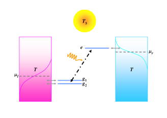
Figure 1: Schematic of a photoelectric converter composed of a three-level QD. The degenerate ground states $|g_{1}\rangle$ and $|g_{2}\rangle$ are coupled to the left-fermionic bath, while the excited state $|e\rangle$ is coupled to the right-fermionic bath. The two fermionic baths are maintained at the same temperature $T$ but have different chemical potentials $\mu_{l}$ and $\mu_{r}=\mu_{l}+qV$ due to the applied voltage ($q$ is the elementary charge). Transitions between the ground states and the excited state are induced by photons with temperature $T_{S}$ (curved arrow).

II GENERAL DESCRIPTION OF THE MODEL

The system schematic (Figure 1) of a photoelectric converter consists of a three-level quantum dot (QD) contacted with two fermionic baths and photons. The three-level QD is modeled by the Hamiltonian

$$H_{S}=\sum_{i=g_{1},g_{2},e,0}\varepsilon_{i}|i\rangle\langle i|,$$ (1)

with $|0\rangle$ being the state for no electron in the QD. $|g_{1}\rangle$, $|g_{2}\rangle$, and $|e\rangle$ represent one-electron states in levels $\varepsilon_{g_{1}}$, $\varepsilon_{g_{2}}$, or $\varepsilon_{e}$, respectively. We assume that Coulomb repulsions prevent two electrons to be simultaneously present in the QD (key-17, ). One electron is firstly transferred from the left-fermionic bath to the ground state $|g_{1}\rangle$ or $|g_{2}\rangle$ via the QD-bath coupling, and then has a probability to be pumped to the excited state $|e\rangle$ due to the incoming solar radiation. The excited state $|e\rangle$ is coupled to the fermionic bath characterized by temperature $T$ and chemical potential $\mu_{r}$.

The Hamiltonian of the sunlight radiation ($R{}_{P}$) is given by

$$H_{P}=\sum_{k\text{$\in R_{P}$}}\omega_{k}a_{k}^{\dagger}a_{k},$$ (2)

where $\omega_{k}$ is the eigenfrequency of the radiated electromagnetic wave described by the creation (annihilation) operator $a{}_{k}^{\dagger}$ $(a{}_{k})$. Similarly, the Hamiltonians of the fermionic baths ($R_{l}$ and $R_{r}$) are given by

$$H_{F}^{l,r}=\sum_{v\in R_{l,r}}\omega_{v}c_{v}^{\dagger}c_{v}.$$ (3)

Here, $c{}_{v}^{\dagger}$ $(c{}_{v})$ is the electron creation (annihilation) operator of the mode $\omega_{v}$ in $R_{l}$ or $R_{r}$. The two ferminoic baths stand for the n-and p-type semiconductor electrodes of the photoelectric converter.

The interaction between the QD and the environment reads $H_{I}=H_{I}^{l}+H_{I}^{r}+H_{I}^{P}$ with each term defined by

$$H_{I}^{l}=\underset{i=1,2}{\sum}\underset{v\in R_{l}}{\sum}(T_{v_{i}}c_{v}|g_{i}\rangle\langle 0|+h.c.),$$ (4)

$$H_{I}^{r}=\underset{v\in R_{r}}{\sum}(T_{v_{e}}c_{v}|e\rangle\langle 0|+h.c.),$$ (5)

and

$$H_{I}^{P}=\underset{i=1,2}{\sum}\underset{k\in R_{P}}{\sum}(g_{k_{i}}a_{k}|e\rangle\langle g_{i}|+h.c.),$$ (6)

where $T_{v_{i}}$, $T_{v_{e}}$, and $g_{k_{i}}$ denote the coupling strength of the transitions between the QD and the left-fermionic bath, the right-fermionic bath and photons, respectively.

III MOTION EQUANTION OF THE QUANTUM DOT

The three-level QD can be viewed as an open quantum system vulnerable to interactions with the environment. Making the Born-Markov approximation, which involves assuming that the environment is time-independent and the environment correlations decay rapidly in comparison to the typical timescale of the system evolution (key-18, ), we derive the equation of motion for the density operator $\rho$ in a Lindblad-like form

$$\overset{.}{\rho}=i[\rho,H_{S}]+\mathcal{L_{\mathrm{\mathit{P}}}\mathrm{[\rho]}}+\mathcal{L_{\mathrm{\mathit{l}}}\mathrm{[\rho]}}+\mathcal{L_{\mathrm{\mathit{r}}}\mathrm{[\rho]}\mathrm{.}}$$ (7)

The dissipative part in the master equation can be generalized into three individual elements including the dampings through the photons and the two fermionic baths. For the photon excitation, the dissipation operator $\mathit{\mathcal{L}_{P}}[\rho]$ depends on the Bose-Einstein statistics of the photons and is given by

$$\mathit{\mathcal{L}_{P}}[\rho] =i[\rho,H_{CP}]$$

$$+\underset{i,j=1}{\overset{2}{\sum}\{[}B_{ij}^{+}(\varepsilon_{j})+B_{ij}^{+}(\varepsilon_{i})][\sigma_{Pi}^{\dagger}\rho\sigma_{Pj}-\frac{1}{2}\{\rho,\sigma_{Pj}\sigma_{Pi}^{\dagger}\}_{+}]$$

$$+[{\textstyle B_{ji}^{-}(\varepsilon_{j})+B_{ji}^{-}(\varepsilon_{i})][\sigma_{Pi}\rho\sigma_{Pj}^{\dagger}-\frac{1}{2}\{\rho,\sigma_{Pj}^{\dagger}\sigma_{Pi}\}_{+}]}\},$$ (8)

where $\sigma_{Pi}=|g_{i}\rangle\langle e|$, $B_{ij}^{+}(\varepsilon_{j})=\gamma_{ij}^{P}(\varepsilon_{j})n(x_{j})$ and $B_{ij}^{-}(\varepsilon_{j})=\gamma_{ij}^{P}(\varepsilon_{j})[1+n(x_{j})]$ are the dissipation rates with $\gamma_{ij}^{P}(\omega)=\pi\sum g_{k_{i}}g_{k_{j}}^{\ast}\delta(\varepsilon-\omega)=[\gamma_{ji}^{P}(\omega)]^{\ast}$; $n(x)=[exp(x)-1]^{-1}$ is the Bose-Einstein distribution with scaled energy $x_{j}=\varepsilon_{j}/(k_{B}T_{P})$ and $k_{B}$ is the Boltzmann constant. The energy difference of each transition is defined as $\varepsilon_{j}=\varepsilon_{e}-\varepsilon_{g_{j}}$. The left-fermionic bath is coupled to the ground states $|g_{1}\rangle$ and $|g_{2}\rangle$. The corresponding dissipation operator is then expressed as

$$\mathit{\mathcal{L}_{l}}[\rho] =i[\rho,H_{Cl}]$$

$$+\underset{i,j=1}{\overset{2}{\sum}\{[}F_{ij}^{l+}(\varepsilon_{g_{j}})+F_{ij}^{l+}(\varepsilon_{g_{i}})][\sigma_{li}^{\dagger}\rho\sigma_{lj}-\frac{1}{2}\{\rho,\sigma_{lj}\sigma_{li}^{\dagger}\}_{+}]$$

$$+[{\textstyle F_{ji}^{l-}(\varepsilon_{g_{j}})+F_{ji}^{l-}(\varepsilon_{g_{i}})][\sigma_{li}\rho\sigma_{lj}^{\dagger}-\frac{1}{2}\{\rho,\sigma_{lj}^{\dagger}\sigma_{li}\}_{+}]}\}.$$ (9)

where $\sigma_{li}=|0\rangle\langle g_{i}|$, $F_{ij}^{l+}(\varepsilon_{g_{j}})=\gamma_{ij}^{l}(\varepsilon_{g_{j}})f(x_{g_{j}})$ and $F_{ij}^{l-}(\varepsilon_{g_{j}})=\gamma_{ij}^{l}(\varepsilon_{g_{j}})[1-f(x_{g_{j}})]$ with $\gamma_{ij}^{l}(\omega)=\pi\sum T_{v_{i}}T_{v_{j}}^{\ast}\delta(\varepsilon-\omega)=[\gamma_{ji}^{l}(\omega)]^{\ast}$; $f(x)=[exp(x)+1]^{-1}$ is the Fermi distribution with scaled energies of the ground states $x_{g_{j}}=(\varepsilon_{g_{j}}-\mu_{l})/(k_{B}T)$. The dissipation operator describes the coupling between the right-fermionic bath and the excited state is

$$\mathit{\mathcal{L}_{r}}[\rho]=F^{r+}(\varepsilon_{e})[2\sigma_{re}^{\dagger}\rho\sigma_{re}-\sigma_{re}\sigma_{re}^{\dagger}\rho-\rho\sigma_{re}\sigma_{re}^{\dagger}]$$

$$+F^{r-}(\varepsilon_{e})[2\sigma_{re}\rho\sigma_{re}^{\dagger}-\sigma_{re}^{\dagger}\sigma_{re}\rho-\rho\sigma_{re}^{\dagger}\sigma_{re}]$$ (10)

where $\sigma_{re}=|0\rangle\langle e|$. $F^{r+}(\varepsilon_{e})=\gamma^{r}(\varepsilon_{e})f(x_{r})$ and $F^{r-}=\gamma^{r}(\varepsilon_{e})[1-f(x_{r})]$ with $\gamma^{r}(\omega)=\pi\sum T_{v_{e}}T_{v_{e}}^{\ast}\delta(\varepsilon-\omega)=[\gamma^{r}(\omega)]^{\ast}$. $x_{r}=(\varepsilon_{e}-\mu_{r})/(k_{B}T)$ is the scaled energy of the excited state.

Notice that the interference of coherent transitions can be simultaneously induced by the photons and the left-fermionic bath, leading to two different non-diagonal couplings given by

$$H_{CP} =\frac{1}{2i}\underset{i,j=1}{\overset{2}{\sum}\{[}B_{ij}^{+}(\varepsilon_{i})-B_{ij}^{+}(\varepsilon_{j})]\sigma_{Pj}\sigma_{Pi}^{\dagger}$$

$$+[{\textstyle B_{ji}^{-}(\varepsilon_{i})-B_{ji}^{-}(\varepsilon_{j})]\sigma_{Pj}^{\dagger}\sigma_{Pi}}\}$$ (11)

and

$$H_{Cl} =\frac{1}{2i}\underset{i,j=1}{\overset{2}{\sum}\{}[F_{ij}^{l+}(\varepsilon_{g_{i}})-F_{ij}^{l+}(\varepsilon_{g_{j}})]\sigma_{lj}\sigma_{li}^{\dagger}$$

$$+[{\textstyle F_{ji}^{l-}(\varepsilon_{g_{i}})-F_{ji}^{l-}(\varepsilon_{g_{j}})]\sigma_{lj}^{\dagger}\sigma_{li}\}}.$$ (12)

According to Eqs. (7)-(10), we have a coupled set of equations describing the dynamics of the populations, $\rho_{i}=\langle g_{i}|\rho|g_{i}\rangle$, $\rho_{e}=\langle e|\rho|e\rangle$, $\rho_{0}=\langle 0|\rho|0\rangle$, and the coherence, $\rho_{ij}=\langle g_{i}|\rho|g_{j}\rangle$, as follows,

$$\overset{.}{\rho}_{1} =-2[B_{11}^{+}(\varepsilon_{1})+F_{11}^{l-}(\varepsilon_{g_{1}})]\rho_{1}+2B_{11}^{-}(\varepsilon_{1})\rho_{e}+2F_{11}^{l+}(\varepsilon_{g_{1}})\rho_{0}$$

$$-[B_{12}^{+}(\varepsilon_{2})+F_{21}^{l-}(\varepsilon_{g_{2}})]\rho_{12}-[B_{21}^{+}(\varepsilon_{2})+F_{12}^{l-}(\varepsilon_{g_{2}})]\rho_{21}$$ (13)

$$\overset{.}{\rho}_{2} =-2[B_{22}^{+}(\varepsilon_{2})+F_{22}^{l-}(\varepsilon_{g_{2}})]\rho_{2}+2B_{22}^{-}(\varepsilon_{2})\rho_{e}+2F_{22}^{l+}(\varepsilon_{g_{2}})\rho_{0}$$

$$-[B_{12}^{+}(\varepsilon_{1})+F_{21}^{l-}(\varepsilon_{g_{1}})]\rho_{12}-[B_{21}^{+}(\varepsilon_{1})+F_{12}^{l-}(\varepsilon_{g_{1}})]\rho_{21}$$ (14)

$$\overset{.}{\rho}_{e} =2B_{11}^{+}(\varepsilon_{1})\rho_{1}+2B_{22}^{+}(\varepsilon_{2})\rho_{2}-2[B_{11}^{-}(\varepsilon_{1})+B_{22}^{-}(\varepsilon_{2})$$

$$+F^{r-}(\varepsilon_{e})]\rho_{e}+2F^{r+}(\varepsilon_{e})\rho_{0}+[B_{12}^{+}(\varepsilon_{1})+B_{12}^{+}(\varepsilon_{2})]\rho_{12}$$

$$+[B_{21}^{+}(\varepsilon_{1})+B_{21}^{+}(\varepsilon_{2})]\rho_{21}$$ (15)

$$\overset{.}{\rho}_{0} =2F_{11}^{l-}(\varepsilon_{g_{1}})\rho_{1}+2F_{22}^{l-}(\varepsilon_{g_{2}})\rho_{2}+2F^{r-}(\varepsilon_{e})\rho_{e}-2[F_{11}^{l+}(\varepsilon_{g_{1}})$$

$$+F_{22}^{l+}(\varepsilon_{g_{2}})+F^{r+}(\varepsilon_{e})]\rho_{0}+[F_{21}^{l-}(\varepsilon_{g_{1}})+F_{21}^{l-}(\varepsilon_{g_{2}})]\rho_{12}$$

$$+[F_{12}^{l-}(\varepsilon_{g_{1}})+F_{12}^{l-}(\varepsilon_{g_{2}})]\rho_{21}$$ (16)

and

$$\overset{.}{\rho}_{12} =-[B_{21}^{+}(\varepsilon_{1})+F_{12}^{l-}(\varepsilon_{g_{1}})]\rho_{1}-[B_{21}^{+}(\varepsilon_{2})+F_{12}^{l-}(\varepsilon_{g_{2}})]\rho_{2}$$

$$+[B_{21}^{-}(\varepsilon_{1})+B_{21}^{-}(\varepsilon_{2})]\rho_{e}+[F_{12}^{l+}(\varepsilon_{g_{1}})+F_{12}^{l+}(\varepsilon_{g_{2}})]\rho_{0}$$

$$-[B_{11}^{+}(\varepsilon_{1})+B_{22}^{+}(\varepsilon_{2})+F_{11}^{l-}(\varepsilon_{g_{1}})+F_{22}^{l-}(\varepsilon_{g_{2}})+\tau]\rho_{12}$$

$$+i\varDelta_{21}\rho_{12}.$$ (17)

Here, $\varDelta_{21}=\varepsilon_{g_{2}}-\varepsilon_{g_{1}}$ is the energy difference of the two lower states $|g_{1}\rangle$ and $|g_{2}\rangle$, and $\tau$ is phenomenologically introduced to describe the decoherence rate due to the environment effects. The equations for off-diagonal terms, e.g. $\langle g_{i}|\rho|e\rangle$ and $\langle e|\rho|0\rangle$, have been omitted except $\rho_{12}$, since those terms only give the decay processes and do not affect the steady-state solution. It is shown that the time evolutions of the populations $\rho_{i}$, $\rho_{e}$, and $\rho_{0}$ are not decoupled from that of the off-diagonal elements $\rho_{12}/\rho_{21}$. The coherence $\rho_{12}/\rho_{21}$ may not vanish even in the steady state after long time evolution. Specifically, we find that both QD-photon coupling and QD-fermion coupling contribute to the coherent transitions.

IV THERMODYNAMIC QUANTITIES AT STEADY STATE

For degenerate lower levels $\varepsilon_{g_{1}}=\varepsilon_{g_{2}}=\varepsilon_{l}$ and symmetric couplings, we write the rates of transitions $|g_{1}\rangle\leftrightarrow|e\rangle$ and $|g_{2}\rangle\leftrightarrow|e\rangle$ as $\gamma_{11}^{P}(\varepsilon_{1})=\gamma_{22}^{P}(\varepsilon_{2})=\gamma^{P}$ and that of transitions $|g_{1}\rangle\leftrightarrow|0\rangle$ and $|g_{2}\rangle\leftrightarrow|0\rangle$ as $\gamma_{11}^{l}(\varepsilon_{g_{1}})=\gamma_{22}^{l}(\varepsilon_{g_{2}})=\gamma^{l}$. We also introduce two dimensionless parameters $r_{P}(=\gamma_{12}^{P}/\gamma^{P})$ and $r_{l}(=\gamma_{12}^{l}/\gamma^{l})$ to describe the strengths of coherences, where superscripts $P$ and $l$ imply the coherent transitions originating from the couplings to the photons and the left-fermionic bath, respectively. Note that $0\leq r_{P},r_{l}$$\leq 1$, depending on the relative orientations of transition dipole vectors (key-15, ). Setting $\stackrel{{\scriptstyle.}}{{\rho}}=0$ and combining Eqs. (13)-(17) with the conservative equation $\rho_{1}+\rho_{2}+\rho_{e}+\rho_{0}=1$, the steady-state populations and coherence of the open quantum system is obtained. The coherence is computed as

$$\rho_{12} =2\gamma^{P}(r_{P}-r_{l})\{n(x_{g})f(x_{l})-[1+n(x_{g})$$

$$-f(x_{l})]f(x_{r})\}/\Omega,$$ (18)

where $\Omega$ is the normalization factor that ensures the sum of probabilities to be equal to unity. Simplifying the numerator of Eq. (18) to $1/2\gamma^{P}(r_{l}-r_{P})\textrm{Csch}(x_{g}/2)\textrm{Sech}(x_{l}/2)\textrm{Sech}(x_{r}/2)\textrm{Sinh}[(x_{g}+x_{l}-x_{r})/2)]$, we identify that $\rho_{12}$ reduces to zero when $r_{P}=r_{l}$ and the quantum coherence will not affect the thermodynamics. This phenomenon was observed in a four-level quantum heat engine for symmetric coupling condition as well (key-16, ).

From the master equation, the changing rate of the electron number in the three-level QD at time $t$ is

$$\overset{.}{\overline{N}}(t)=\mathrm{Tr}\{n\mathcal{L_{\mathrm{\mathit{l}}}\mathrm{[\rho]}}\}+\mathrm{Tr}\{n\mathcal{L_{\mathrm{\mathit{r}}}\mathrm{[\rho]}}\}\coloneqq J_{l}+J_{r}$$ (19)

with the number operator $n=\sigma_{re}^{\dagger}\sigma_{re}+\sigma_{l1}^{\dagger}\sigma_{l1}+\sigma_{l2}^{\dagger}\sigma_{l2}$. Thus, $J_{l}$ and $J_{r}$ are the currents exchanging with the left and the right fermionic baths, which are given by

$$J_{l}=4\gamma^{l}f(x_{l})\rho_{0}-2\gamma^{l}[1-f(x_{l})]\{\rho_{1}+\rho_{2}+r_{l}\mathrm{Re[}\rho_{12}]\}$$ (20)

and

$$J_{r}=2\gamma^{r}[1-f(x_{r})]\rho_{e}-2\gamma^{r}f(x_{r})\rho_{0}.$$ (21)

The parameter, $x_{l}=(\varepsilon_{l}-\mu_{l})/(k_{B}T)$, is the scaled energy of the degenerate ground states. In the stationary state $(t\rightarrow\text{$\infty$})$, $\overset{.}{N}(t)=0$ such that $J_{l}=-J_{r}$. Eq. (20) indicates that adjusting the electron current via quantum coherences allows for improving the performance of the converter. The steady state energy fluxes are determined by energy change of the three-level QD, i.e. $\overset{.}{E}(\text{$\infty$})=\mathrm{Tr}\{H_{S}\overset{.}{\rho}(\text{$\infty$})\}=\underset{\alpha}{\sum}\mathrm{Tr}\{H_{S}\mathcal{L}_{\alpha}[\rho(\text{$\infty$})]\}$ ($\alpha=P$, $l$, and $r$ ). Neglecting the nonradiative recombination processes (key-11, ; key-20, ), the net heat flux coming from the sunlight $\overset{.}{Q}_{P}=\mathrm{Tr}\{H_{S}\mathcal{L}_{P}[\rho(\text{$\infty$})]\}=\varepsilon_{g}J$, where $\varepsilon_{g}=\varepsilon_{e}-\varepsilon_{l}$ can be regarded as the bandgap energy. The power $P$ generated by the photoelectric converter to move electrons from the left-fermionic bath to the right-fermionic bath yields

$$P=(\mu_{r}-\mu_{l})J=k_{B}T_{P}[x_{g}-(1-\eta_{c})(x_{r}-x_{l})]J$$ (22)

with $x_{g}=\varepsilon_{g}/(k_{B}T_{P})$. The symbol $\eta_{c}$ denotes the Carnot efficiency and equals $1-T/T_{P}$. The efficiency satisfying this conversion is then given by

$$\eta=\frac{P}{\overset{.}{Q}_{P}}=\frac{(\mu_{r}-\mu_{l})J}{\varepsilon_{g}J}=1-(1-\eta_{c})\frac{(x_{r}-x_{l})}{x_{g}}.$$ (23)

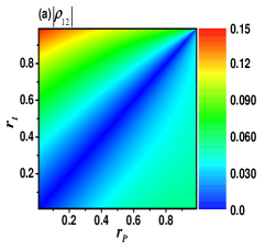
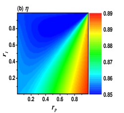
Figure 2: The absolute value of coherence (a) and the efficiency (b) as a function of the dimensionless parameters $r_{P}$ and $r_{l}$, where $x_{g}=2,$ $\tau=0$, $T=295K$, and $T_{P}=5780K$. The optimal values of $x_{l}$ and $x_{r}$ have been computed numerically to maximize the power output.

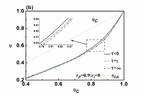
Figure 3: The efficiency at maximum power and the Curzon-Ahlborn efficiency (green dashed line) as a function of Carnot efficiency $\eta_{c}$ for different values of $r_{l}$ (a) and $\tau$ (b). In Fig. 3a, $r_{P}=0.9$ and $\tau=0$. In Fig. 3b, $r_{P}=0.9$ and $r_{l}=0$. The inserted figure shows an enlargement of the representative part of each plot.

V PERFORMANCE CHARACTERISTIC ANALYSIS

In the following section, we address the question regarding the extent to which the quantum nature of the converter affects the photoelectric conversion efficiency, a topic which is beyond the reach of the model presented in Refs. [11]. The formalism obtained here will allow us to access how coherences can lead to an enhancement of the power and the efficiency. To do so, we parameterize the transition rates $\gamma^{P}=\gamma^{l}=\gamma^{r}$=$\gamma$ without loss of generality.

Figures 2a and 2b show the contour plots of the absolute value of coherence $\mid\rho_{12}\mid$ and the efficiency $\eta$ versus $r_{P}$ and $r_{l}$, where the power has been optimized with respect to $x_{l}$ and $x_{r}$. In accordance with the requirements set out in the analytical method (Eq. 18), Fig. 2a shows that the quantum coherence vanishes if $r_{P}=r_{l}$, resulting in low efficiency less than $0.87$. To enhance $\eta$ in the presence of coherence $(\mid\rho_{12}\mid\neq 0)$, $r_{P}$ and $r_{l}$ should be designed to be different from each other. However, we notice that $\eta$ and $\mid\rho_{12}\mid$ may not always increase or decrease together, which means that $\eta$ is not only restricted by the magnitude of coherence. Comparing Fig. 2a with Fig. 2b, we find that $\eta$ can be largely enhanced in the range of $r_{P}>r_{l}$. This condition suggests that increasing the coherence coupling between the QD and the photons and $\mid\rho_{12}\mid$ will concurrently benefit the performance of the photoelectric conversion. There exists a perfect positive correlation between $\eta$ and $\mid\rho_{12}\mid$ when $r_{P}>r_{l}$ is satisfied.

Next, we maximize the power with respect to $x_{g}$ , $x_{l}$ , and $x_{r}$. In Figure 3a, the efficiency at maximum power is plotted as a function of $\eta_{c}$ for given values of $r_{P}$. Figure 3a shows that the efficiency at maximum power increases with a decrease in the parameter $r_{l}$, as expected. When $r_{P}=r_{l}=0.9$ (dash-dotted line), the efficiency remains close to the Curzon-Ahlborn efficiency for almost all values of $\eta_{c}$. Slight lower efficiencies are observed only far from equilibrium where $\eta_{c}$ is large. These features have also been addressed in other approaches to non-equilibrium thermodynamics, such as Brownian heat engine (key-21, ; key-22, ), Feynman ratchet model (key-23, ), and thermoelectric device (key-24, ), and therefore point to a fundamental principle that can be associated with the presence of inherently irreversible dynamics when device is operated at maximum power.

Intriguingly, we find that the efficiency at maximum power is not limited by the Curzon-Ahlborn efficiency. For example, when $r_{l}=0.3$ (short-dashed line) or $r_{l}=0$ (solid line), the quantum coherence appears and the efficiency at maximum power will exceed the bound given by the Curzon-Ahlborn efficiency. These results are remarkable in our model with quantum coherence. The quantum coherence will redistribute the population in the three-level QD and accelerate the removal of electrons, thus increasing the number of absorbed photons and reducing recombination losses.

Finally, we consider the typical problem arising due to the decoherence. Decoherence occurs when a system interacts with its environment in a thermodynamically irreversible way. The decoherence processes can drastically decrease an engine’s efficiency. In Fig. 3b, the efficiency at maximum power is plotted as a function of $\eta_{c}$ with $r_{P}=0.9$ and $r_{l}=0$. In the case that the decoherence rate is extremely large, i.e., $\tau\rightarrow\infty$, the efficiency (dashed line) again becomes slightly lower than the Curzon-Ahlborn efficiency. As $\tau$ diminishes, we find that the efficiency increases monotonically. The efficiency at maximum power is significantly higher than the Curzon-Ahlborn efficiency when $\tau=0$.

VI CONCLUDSIONS

In summary, we propose a new type of photoelectric converter, which consists of a three-level QD coupling to two fermionic baths and sunlight radiation. It follows from the Born-Markov approximation that the interference due to coherent transitions can be simultaneously induced by the sunlight and the left-fermionic bath, leading to two different non-diagonal Lamb shifts in the Lindblad-like master equation. The results of the thermodynamic analysis show that the quantum coherence is capable of improving the efficiency beyond the limit of a system whose quantum effects are absent. The application of quantum mechanics will bring new insight to understand the fundamantal problem in thermodynamics when it is applied to the nano-electronic systems.

References

• (1) M. O. Scully, M. S. Zubairy, G. S. Agarwal, and H. Walther, Science 299, 862-864 (2003).
• (2) J. Roßnagel, O. Abah, F. Schmidt-Kaler, K. Singer, and E. Lutz, Phys. Rev. Lett. 112, 030602 (2014).
• (3) X. L. Huang, Tao Wang, and X. X. Yi, Phys. Rev. E 86, 051105 (2012).
• (4) H. T. Quan, P. Zhang, and C. P. Sun, Phys. Rev. E 73, 036122 (2006).
• (5) R. S. Whitney, Phys. Rev. Lett. 112, 130601 (2014).
• (6) M. Esposito, R. Kawai, K. Lindenberg, and C. Van den Broeck, Phys. Rev. Lett. 105, 150603 (2010).
• (7) F.L. Curzon and B. Ahlborn, Am. J. Phys. 43, 22-24 (1975).
• (8) J. Wang, Z. Ye, Y. Lai, W. Li, and J. He, Phys. Rev. E 91, 062134 (2015);
• (9) F. Wu, J. He, Y. Ma, and J. Wang, Phys. Rev. E 90, 062134 (2014).
• (10) J. Guo, J. Wang, Y. Wang, and J. Chen, Phys. Rev. E 87, 012133 (2013).
• (11) B. Rutten, M. Esposito, and B. Cleuren, Phys. Rev. B 80, 235122 (2009).
• (12) S. W. Li, C. Y. Cai, and C. P. Sun, Ann. Phys. -New York 360, 19-32 (2015).
• (13) M. O. Scully, K. R. Chapin, K. E. Dorfman, M. B. Kim, and A. Svidzinsky, Proc. Natl. Acad. Sci. U.S.A. 108, 15097-15100 (2011).
• (14) K. E. Dorfman, D. V. Voronine, S. Mukamel, and M. O. Scully, Proc. Natl. Acad. Sci. USA 110, 2746-2751 (2013).
• (15) U. Harbola, S. Rahav, and S. Mukamel, EPL 99, 50005 (2012).
• (16) H. P. Goswami and U. Harbola, Phys. Rev. A 88, 013842 (2013).
• (17) B. Cleuren, B. Rutten, and C. Van den Broeck, Phys. Rev. Lett. 108, 120603 (2012).
• (18) H. P. Breuer and F. Petruccione, The theory of open quantum systems (Oxford University Press, Oxford, 2001).
• (19) J. Wang, Y. Lai, Z. Ye, J. He, Y. Ma, and Q. Liao, Phys. Rev. E 91, 050102(R) (2015).
• (20) V. Blickle and C. Bechinger, Nat. Phys. 8, 143–146 (2012).
• (21) Z. C. Tu, Phys. Rev. E 89, 052148 (2014).
• (22) Z. C. Tu, J. Phys. A 41, 312003 (2008).
• (23) M Esposito, K Lindenberg, and C. Van den Broeck, EPL 85, 60010 (2009).