Functional summary statistics for point processes on the sphere with an application to determinantal point processes

Abstract

We study point processes on $\mathbb{S}^{d}$, the $d$-dimensional unit sphere $\mathbb{S}^{d}$, considering both the isotropic and the anisotropic case, and focusing mostly on the spherical case $d=2$. The first part studies reduced Palm distributions and functional summary statistics, including nearest neighbour functions, empty space functions, and Ripley’s and inhomogeneous $K$-functions. The second part partly discusses the appealing properties of determinantal point process (DPP) models on the sphere and partly considers the application of functional summary statistics to DPPs. In fact DPPs exhibit repulsiveness, but we also use them together with certain dependent thinnings when constructing point process models on the sphere with aggregation on the large scale and regularity on the small scale. We conclude with a discussion on future work on statistics for spatial point processes on the sphere.

aggregation; empty space function; inhomogeneous $K$-function; isotropic covariance function; joint intensities; likelihood; nearest neighbour function; Palm distribution; repulsiveness; spectral representation.

1 Introduction

1.1 Aim and motivation

How do we construct models and functional summary statistics for spatial point processes on the $d$-dimensional unit sphere $\mathbb{S}^{d}\subset\mathbb{R}^{d+1}$ when their realizations exhibit aggregation or regularity or perhaps a combination of both? Here $d=1,2$ are the practically most relevant cases and for specificity we let $d=2$ in this paper, noting that $\mathbb{S}^{2}$ apart from a scaling may be considered as an approximation of planet Earth. However, our discussion can easily be extended to point processes on $\mathbb{S}^{1}$ and the general case of $\mathbb{S}^{d}$ may be covered as well.

The first part concerns point processes on $\mathbb{S}^{2}$ (Section 2) and in particular Palm distributions and functional summary statistics (Section 3). In the isotropic case of a point process on the sphere, [31] studied an extension of Ripley’s $K$-function to the sphere without providing the mathematical details for the reduced Palm distribution, which they first use in their definition of the $K$-function on the sphere and second relate to the second order intensity (or pair correlation) function without any proof. We provide this definition without assuming isotropy so that the inhomogeneous $K$-function, introduced in [1] for point processes on Euclidean spaces, can be defined on the sphere as well. Moreover, in the isotropic case, we introduce further useful functional summary functions, namely the nearest neighbour function, the empty space function, and the related so-called $J$-function.

The second part partly reviews the attractive properties of determinantal point process (DPP) models on the sphere and considers the application of functional summary statistics to DPPs. Briefly, DPPs offer relatively flexible models for repulsiveness (although less flexible than Gibbs point processes), they can be easily simulated, and their moments and the likelihood are tractable, cf. [10, 14, 15]. They have mostly been studied and applied for point processes on $\mathbb{R}^{d}$, though many results can easily be adapted or may even be simpler for point processes on $\mathbb{S}^{d}$, cf. [21]. They are of interest because of their applications in mathematical physics, combinatorics, random-matrix theory, machine learning, and spatial statistics (see [15] and the references therein). Simulated examples of DPPs on the sphere with various degrees of repulsiveness are shown in Figure 1.

Figure 1: Northern Hemisphere of three spherical point patterns projected to the unit disc with an equal-area azimuthal projection. Each pattern is a simulated realization of a determinantal point process on the sphere with mean number of points 225. Left: Complete spatial randomness (Poisson process). Middle: Multiquadric model with $\tau=10$ and $\delta=\nobreak 0.68$. Right: Most repulsive DPP.

Finally, Section 5 contains our concluding remarks, including a discussion on future work on statistics for spatial point processes on the sphere.

1.2 Related work and software

When we had completed the first version of this paper (see [22]) we realized that similar independent research on functional summary statistics by [17] was submitted to another journal at the same time as our work, but their paper and our paper supplement each other in different ways: [17] analyze data fitted by a model for clustering (a so-called Thomas process where for the offspring distribution a von Mises-Fisher distribution on the sphere is replacing the bivariate normal distribution used for a planar Thomas process), while we instead consider DPPs which model regularity. While we provide the details on Palm distributions, they discuss edge correction factors for the functional summary statistics in more detail than we do how. Moreover, partly following [16], we use DPPs together with certain dependent thinnings when constructing point process models with aggregation on the large scale and regularity on the small scale. Our paper also provides a survey of and a supplement to [21], which deals with DPPs on $\mathbb{S}^{d}$, and where in the present paper we attempt to give a less technical exposition for $d=2$.

In connection to this paper, the development of software for simulation of DPPs on the sphere and calculation of non-parametric estimators for the functional summary statistics constitutes a substantial amount of work. The software is written in the R language [27] and will be available as an extension of the spatstat package [2]. Section 3 shows examples of how to use the software and the type of plots it can produce.

2 Point processes on the sphere

Throughout this paper we use a notation and make assumptions as follows.

Consider a simple finite point process $\bm{X}$ on $\mathbb{S}^{2}$, i.e., we can view $\bm{X}$ as a random finite subset of $\mathbb{S}^{2}$. Let $N$ be its corresponding counting measure, i.e., $N(A)$ denotes the number of points in $\bm{X}$ falling in a region $A\subseteq\mathbb{S}^{2}$. The state space for $X$ is then the set of all finite subsets of $\mathbb{S}^{2}$ equipped with the $\sigma$-algebra $\mathcal{F}$ generated by the events $\{N(A)=n\}$ for Borel sets $A\subseteq\mathbb{S}^{2}$ and integers $n=0,1,\ldots$.

For

$$\bm{x}=(x_{1},x_{2},x_{3})=(\sin\vartheta\cos\varphi,\sin\vartheta\sin\varphi,\cos\vartheta)\in\mathbb{S}^{2}$$ (2.1)

where $\vartheta\in[0,\pi]$ is the polar latitude and $\varphi\in[0,2\pi)$ is the polar longitude, let

$$\mathrm{d}\nu(\bm{x})=\sin\vartheta\,\mathrm{d}\varphi\,\mathrm{d}\vartheta$$ (2.2)

be the surface measure on $\mathbb{S}^{2}$. Suppose $\rho:\mathbb{S}^{2}\mapsto[0,\infty)$ is a Borel function so that $a:=\int_{\mathbb{S}^{2}}\rho(\bm{x})\,\mathrm{d}\nu(\bm{x})$ is finite. Then $\bm{X}$ is a Poisson process with intensity function $\rho$ if $N:=N(\mathbb{S}^{2})$ is Poisson distributed with parameter $a$, and if conditional on $N=n$, the $n$ points in $\bm{X}$ are independent and each point has density proportional to $\rho$. A Poisson process is the case of no interaction, i.e., it is neither clustered nor repulsive/inhibitive.

For $n=1,2,\ldots$, we say that $\bm{X}$ has $n$th order joint intensity $\rho^{(n)}:(\mathbb{S}^{2})^{n}\mapsto[0,\infty)$ with respect to the $n$-fold product surface measure $\nu^{(n)}=\nu\times\dots\times\nu$ if for any Borel function $h:(\mathbb{S}^{2})^{n}\mapsto[0,\infty)$,

$$\mathrm{E}\sum_{\bm{x}_{1},\ldots,\bm{x}_{n}\in\bm{X}}^{\not=}h(\bm{x}_{1},\ldots,\bm{x}_{n})=\int h(\bm{x}_{1},\ldots,\bm{x}_{n})\rho^{(n)}(\bm{x}_{1},\ldots,\bm{x}_{n})\,\mathrm{d}\nu^{(n)}(\bm{x}_{1},\ldots,\bm{x}_{n})$$ (2.3)

and $\int\rho^{(n)}\,\mathrm{d}\nu^{(n)}<\infty$, where the expectation is with respect to $\bm{X}$ and $\not=$ over the summation sign means that $\bm{x}_{1},\ldots,\bm{x}_{n}$ are pairwise distinct. Intuitively, if $\bm{x}_{1},\ldots,\bm{x}_{n}$ are pairwise distinct points on $\mathbb{S}^{2}$, then $\rho^{(n)}(\bm{x}_{1},\ldots,\bm{x}_{n})\,\mathrm{d}\nu^{(n)}(\bm{x}_{1},\ldots,\bm{x}_{n})$ is the probability that $\bm{X}$ has a point in each of $n$ infinitesimally small regions on $\mathbb{S}^{2}$ around $\bm{x}_{1},\ldots,\bm{x}_{n}$ and of surface measure $\mathrm{d}\nu(\bm{x}_{1}),\ldots,\mathrm{d}\nu(\bm{x}_{n})$, respectively, cf. (2.3). Note that $\rho^{(n)}$ is uniquely determined except on a $\nu^{(n)}$-nullset. In particular, $\rho(\bm{x})=\rho^{(1)}(\bm{x})$ is the intensity function (with respect to surface measure) and we define the pair correlation function by

$$g(\bm{x},\bm{y}):=\frac{\rho^{(2)}(\bm{x},\bm{y})}{\rho(\bm{x})\rho(\bm{y})}\qquad\text{if $\rho(\bm{x})\rho(\bm{y})>0$}.$$

The definition of $g(\bm{x},\bm{y})$ when $\rho(\bm{x})\rho(\bm{y})=0$ depends on the particular model of $\bm{X}$ and is mainly only of importance when considering plots of $g$: If $\bm{X}$ is a Poisson process with intensity function $\rho$, then $\rho^{(n)}(\bm{x}_{1},\ldots,\bm{x}_{n})=\rho(\bm{x}_{1})\cdots\rho(\bm{x}_{n})$ and $g(\bm{x},\bm{y})=1$ if $\rho(\bm{x})\rho(\bm{y})>0$, so it is natural to let $g(\bm{x},\bm{y})=1$ if $\rho(\bm{x})\rho(\bm{y})=0$. As we shall see later, for DPPs it is natural to make another choice.

Denote $\mathcal{O}(3)$ the orthogonal group, i.e., the set of all $3\times 3$ matrices $O$ so that $OO^{\top}=O^{\top}O=I$, where $O^{\top}$ is the transpose of $O$ and $I$ is the $3\times 3$ identity matrix. Set $O\bm{X}=\{O\bm{x}:\bm{x}\in\bm{X}\}$. We say that $\bm{X}$ is isotropic/homogeneous if $O\bm{X}$ is distributed as $\bm{X}$ for all $O\in\mathcal{O}(3)$. Then any point in $\bm{X}$ is uniformly distributed on $\mathbb{S}^{2}$, and the intensity function is equal to a constant called the intensity and which we also denote by $\rho$.

3 Palm distributions and functional summary statistics

The most popular functional summary statistic for a stationary point process on $\mathbb{R}^{2}$ with intensity $\rho$ is Ripley’s $K$-function [30], where $\rho K(t)$ is interpreted as the mean number of further points within distance $t$ of a typical point in the process. The formal definition of $K$ requires Palm measure theory, and its definition can be extended to the inhomogeneous $K$-function for so-called second order intensity reweighted stationary point processes [1, 4]. The adaption of Ripley’s $K$-function to a general isotropic point process on the sphere is given in [31], without explicitly specifying the reduced Palm distribution which is needed in the precise definition. In fact $\mathbb{S}^{2}$ is a so-called homogeneous space and reduced Palm distributions for homogeneous spaces have been studied in [32, 13], but instead of applying this technical setting we derive the reduced Palm distributions from first principles.

Section 3.1 gives a definition of the reduced Palm distributions without assuming isotropy and Section 3.2 provides the formal definition of Ripley’s $K$-function, the inhomogeneous $K$-function, and the nearest-neighbour function on the sphere, together with various useful interpretations and results for non-parametric estimation. Later Section 4.4 relates all this to DPPs.

3.1 Palm distribution for a point process on the sphere

Suppose $\bm{X}$ is a point process on $\mathbb{S}^{2}$ with an integrable intensity function $\rho$. The so-called Campbell-Mecke formula gives that for any $\bm{x}\in\mathbb{S}^{2}$ there exists a finite point process $\bm{X}^{!}_{\bm{x}}$ so that

$$\mathrm{E}\sum_{\bm{x}\in\bm{X}}h(\bm{x},\bm{X}\setminus\{\bm{x}\})=\int\mathrm{E}h(\bm{x},\bm{X}^{!}_{\bm{x}})\rho(\bm{x})\,\mathrm{d}\nu(\bm{x})$$ (3.1)

for any non-negative Borel function $h$. Moreover, the distribution of $\bm{X}^{!}_{\bm{x}}$ is unique for $\nu$ almost all $\bm{x}$ with $\rho(\bm{x})>0$, and it is called the reduced Palm distribution at the point $\bm{x}$. If $\rho(\bm{x})=0$, this distribution can be chosen to be arbitrary, since this case will play no role in this paper. Equation (3.1) and the uniqueness result follow from a general result in [8, Proposition 13.1.IV] (noticing that $\bm{X}^{!}_{\bm{x}}\cup\{\bm{x}\}$ follows what they call the local Palm distribution).

Intuitively, $\bm{X}^{!}_{\bm{x}}$ follows the conditional distribution of $\bm{X}\setminus\{\bm{x}\}$ given that $\bm{x}\in\bm{X}$. This interpretation follows from (3.1) or perhaps more easily by assuming that $\bm{X}$ has a density $f$ (with respect to the unit rate Poisson process on $\mathbb{S}^{2}$) since, for $\rho(\bm{x})>0$, $\bm{X}^{!}_{\bm{x}}$ has density

$$f^{!}_{\bm{x}}(\{\bm{x}_{1},\ldots,\bm{x}_{n}\})=f(\{\bm{x},\bm{x}_{1},\ldots,\bm{x}_{n}\})/\rho(\bm{x}).$$

For example, for a Poisson point process with intensity function $\rho$,

$$f(\{\bm{x}_{1},\dots,\bm{x}_{n}\})=\exp\left(4\pi-\int_{\mathbb{S}^{2}}\rho(\bm{x})\,\mathrm{d}\nu(\bm{x})\right)\prod_{i=1}^{n}\rho(\bm{x}_{i})$$

and so it follows that $\bm{X}^{!}_{\bm{x}}$ is distributed as $\bm{X}$ whenever $\rho(\bm{x})>0$. Another example is a log Gaussian Cox process (LGCP) $\bm{X}$ on the sphere with underlying Gaussian process $\bm{Y}=\{\bm{Y}(\bm{x}):\bm{x}\in\mathbb{S}^{2}\}$, i.e., when $\bm{X}$ conditional on $\bm{Y}$ is a Poisson process with intensity function $\exp(\bm{Y}(\bm{x}))$ such that this is almost surely integrable with respect to $\nu$. If $\xi$ and $c$ are the mean and covariance functions of $\bm{Y}$, then $\bm{X}_{\bm{x}}^{!}$ is a LGCP where the underlying Gaussian process has mean function $\xi_{\bm{x}}(\bm{y})=\xi(\bm{y})+c(\bm{x},\bm{y})$ and the same covariance function $c$. This follows along similar lines as in [5].

Assuming $\bm{X}$ is isotropic with intensity $\rho>0$, the situation simplifies as follows. Denote $\mathcal{SO}(3)$ the 3D rotation group, i.e., $O\in\mathcal{SO}(3)$ if and only if $O\in\mathcal{O}(3)$ and $\det O=1$. [17] claim without any proof that for any $\bm{x}\in\mathbb{S}^{2}$ and $R\in\mathcal{SO}(3)$, $\bm{X}^{!}_{R\bm{x}}$ is then distributed as $R\bm{X}^{!}_{\bm{x}}$. We can easily verify this under a mild condition, namely that the distribution of $\bm{X}$ is given by a density $f$ with respect to the unit rate Poisson process on $\mathbb{S}^{2}$ (in other words it is absolutely continuous with respect to this Poisson process). Then

$$f^{!}_{R\bm{x}}(\{\bm{x}_{1},\ldots,\bm{x}_{n}\}) =f(\{\bm{x}_{1},\ldots,\bm{x}_{n},R\bm{x}\})/\rho$$

$$=f(\{R^{\top}\bm{x}_{1},\ldots,R^{\top}\bm{x}_{n},R^{\top}R\bm{x}\})/\rho$$

$$=f^{!}_{\bm{x}}(R^{\top}\{\bm{x}_{1},\ldots,\bm{x}_{n}\})$$

where in the second identity we use that $f$ is invariant under rotations since $\bm{X}$ is isotropic, and hence the claim is verified. So it remains to understand what the distribution of $\bm{X}^{!}_{\mathbf{e}}$ is for an arbitrary fixed point $\mathbf{e}$ on the sphere; in the sequel we choose this to be the North pole $\mathbf{e}=(0,0,1)$.

For $\bm{x}\in\mathbb{S}^{2}\setminus\{\mathbf{e}\}$, there is a unique $R_{\bm{x}}\in\mathcal{SO}(3)$ so that $R_{\bm{x}}\mathbf{e}=\bm{x}$ and its axis of rotation is orthogonal to the great circle on $\mathbb{S}^{2}$ which contains $\bm{x}$ and $\mathbf{e}$. The axis of rotation is given by $\bm{u}(\bm{x})=\frac{\mathbf{e}\times\bm{x}}{\lVert\mathbf{e}\times\bm{x}\rVert}$, where $\times$ denotes the cross product in $\mathbb{R}^{3}$. According to the right hand rule, let $\theta(\bm{x})\in(0,2\pi)$ denote the angle for the rotation $R_{\bm{x}}$ around $\bm{u}(\bm{x})$, i.e., $\theta(\bm{x})=s(\mathbf{e},\bm{x})$ if $0<\theta(\bm{x})\leq\pi$ and $\theta(\bm{x})=2\pi-s(\mathbf{e},\bm{x})$ otherwise, where $s(\mathbf{e},\bm{x})=\arccos(\mathbf{e}\cdot\bm{x})$ denotes great circle distance from $\mathbf{e}$ to $\bm{x}$ and $\cdot$ is the usual inner product on $\mathbb{R}^{3}$. Then $\bm{x}$ is in one-to-one correspondence to $(\theta(\bm{x}),\bm{u}(\bm{x}))$, and by Rodrigues’ rotation formula, for any $\bm{v}\in\mathbb{R}^{3}$,

$$R_{\bm{x}}\bm{v}=\cos\theta(\bm{x})\bm{v}+\sin\theta(\bm{x})(\bm{u}(\bm{x})\times\bm{v})+(1-\cos\theta(\bm{x}))(\bm{u}(\bm{x})\cdot\bm{v})\bm{u}(\bm{x}).$$

Furthermore, define $R_{\mathbf{e}}=I$. Now, when $R^{\top}_{\bm{x}}\bm{X}^{!}_{\bm{x}}$ and $\bm{X}^{!}_{\mathbf{e}}$ are identically distributed it follows from (3.1) that

$$\mathrm{P}\left(\bm{X}^{!}_{\mathbf{e}}\in F\right)=\frac{1}{\nu(A)\rho}\,\mathrm{E}\sum_{\bm{x}\in\bm{X}\cap A}1\left[R_{\bm{x}}^{\top}(\bm{X}\setminus\{\bm{x}\})\in F\right]$$ (3.2)

for $F\in\mathcal{F}$ and an arbitrary Borel set $A\subseteq\mathbb{S}^{2}$ with $\nu(A)>0$. The following proposition summarizes our results.

Proposition 1. Suppose $\bm{X}$ is isotropic with intensity $\rho>0$ and its distribution is absolutely continuous with respect to the unit rate Poisson process on $\mathbb{S}^{2}$. Then for $\nu$ almost all $\bm{x}\in\mathbb{S}^{2}$, $\bm{X}^{!}_{\bm{x}}$ is distributed as $R_{\bm{x}}\bm{X}^{!}_{\mathbf{e}}$, where the distribution of $\bm{X}^{!}_{\mathbf{e}}$ is given by (3.2). So if $k$ is a non-negative measurable function, then for $\nu$ almost all $\bm{x}\in\mathbb{S}^{2}$,

$$\mathrm{E}k\left(R^{\top}_{\bm{x}}\bm{X}^{!}_{\bm{x}}\right)=\mathrm{E}k\left(\bm{X}^{!}_{\mathrm{e}}\right).$$ (3.3)

The absolute continuity condition in Proposition 1 will be satisfied for all point process models we have in mind, but the proposition extends to the general case where absolute continuity is not assumed and $R^{\top}_{\bm{x}}$ in (3.2) is replaced by a uniformly distributed rotation given that it maps $\bm{x}$ to $\mathbf{e}$. The proof, which kindly has been provided by Markus Kiderlen, is deferred to Appendix A.

Henceforth, for ease of presentation we ignore that our statements about $\bm{X}^{!}_{\bm{x}}$ only hold for $\nu$ almost all $\bm{x}\in\mathbb{S}^{2}$.

3.2 Functional summary statistics for isotropic and second order intensity reweighted isotropic point processes on the sphere

3.2.1 The homogeneous case

Assume $\bm{X}$ is an isotropic point process on $\mathbb{S}^{2}$ with intensity $\rho>0$ and its distribution is absolutely continuous with respect to the unit rate Poisson process on $\mathbb{S}^{2}$. Denote geodesic (or orthodromic or great-circle) distance on the sphere by

$$s(\bm{x},\bm{y})=\arccos(\bm{x}\cdot\bm{y}),\qquad\text{$\bm{x},\bm{y}\in\mathbb{S}^{2}$}.$$

Let $s(A,B)=\inf_{\bm{x}\in A,\bm{y}\in B}s(\bm{x},\bm{y})$ be the shortest geodesic distance between $A,B\subset\mathbb{S}^{2}$ and define the nearest neighbour function by

$$G(t)=\mathrm{P}\left(s(\bm{X}^{!}_{\mathbf{e}},\mathbf{e})\leq t\right)=\mathrm{P}\left(s(\bm{X}^{!}_{\bm{x}},\bm{x})\leq t\right),\qquad\text{$0\leq t\leq\pi,\ \bm{x}\in\mathbb{S}^{2}$},$$

where the last identity follows from Proposition 1. Thus $G$ is the distribution function for the geodesic distance from a typical point to the nearest other point in $\bm{X}$. Furthermore, for an arbitrary point $\bm{x}\in\mathbb{S}^{2}$, we define the empty space function by

$$F(t)=\mathrm{P}\left(s(\bm{X},\bm{x})\leq t\right),\qquad\text{$0\leq t\leq\pi$},$$

and following [18], we define the $J$-function by

$$J(t)=\frac{1-G(t)}{1-F(t)}\qquad\text{for $F(t)<1$}.$$

Since $\bm{X}$ is isotropic, $F$ does not depend on the choice of $\bm{x}$. If $\bm{X}$ is a homogeneous Poisson process, then $F_{\mathrm{Pois}}(t)=G_{\mathrm{Pois}}(t)=\exp(-2\pi\rho(1-\cos t))$ and $J_{\mathrm{Pois}}=1$.

Note that for any Borel set $A\subseteq\mathbb{S}^{2}$,

$$\rho\nu(A)G(t)=\mathrm{E}\sum_{\bm{x}\in\bm{X}\cap A}1\left[s(\bm{X}\setminus\{\bm{x}\},\bm{x})\leq t\right].$$

Thinking of $A$ as an observation window, this is a useful result when deriving non-parametric estimates: Let $\mathcal{G}\subset\mathbb{S}^{2}$ be a finite grid of $m>0$ points. If $\bm{X}$ is fully observed on $\mathbb{S}^{2}$, i.e., $A=\mathbb{S}^{2}$, then natural estimates are

$$\widehat{F}(t)=\frac{1}{m}\sum_{\bm{x}\in\mathcal{G}}1\left[s(\bm{X},\bm{x})\leq t\right]$$

and

$$\widehat{G}(t)=\frac{1}{N}\sum_{\bm{x}\in\bm{X}}1\left[s(\bm{X}\setminus\{\bm{x}\},\bm{x})\leq t\right]$$

provided $N=N(\mathbb{S}^{2})>0$. In case the observation window $A$ is a proper subset of $\mathbb{S}^{2}$, minus sampling may be used: Let $A_{\ominus t}=\{\bm{x}\in A:s(\mathbb{S}^{2}\setminus A,\bm{x})>t\}$ be the set of those points in $A$ with geodesic distance at least $t$ to any point outside $A$. Then minus sampling gives the estimate

$$\widehat{G}(t)=\frac{1}{N(A_{\ominus t})}\sum_{\bm{x}\in\bm{X}\cap A_{\ominus t}}1[s(\bm{X},\bm{x})\leq t]$$

provided $N(A_{\ominus t})>0$. Moreover, for $\widehat{F}$ we choose the grid so that $\mathcal{G}\subset A_{\ominus t}$.

Now, we define the $K$-function by

$$K(t)=\frac{1}{\rho}\mathrm{E}\sum_{\bm{x}\in\bm{X}_{\mathbf{e}}^{!}}1\left[s(\mathbf{e},\bm{x})\leq t\right]=\frac{1}{\rho}\mathrm{E}\sum_{\bm{y}\in\bm{X}^{!}_{\bm{x}}}1[s(\bm{x},\bm{y})\leq t],\qquad\text{$0\leq t\leq\pi,\ \bm{x}\in\mathbb{S}^{2}$},$$ (3.4)

where the last equality follows from Proposition 1. We have that

$$\rho K(t)=\mathrm{E}\sum_{\bm{y}\in\bm{X}^{!}_{\bm{x}}}1[s(\bm{x},\bm{y})\leq t]$$ (3.5)

is the mean number of further points within geodesic distance $t$ of a typical point in the process. Furthermore, by Proposition 1 and (3.4), we obtain

$$\rho^{2}\nu(A)K(t)=\mathrm{E}\sum_{\bm{x}\in\bm{X}\cap A}\sum_{\bm{y}\in\bm{X}\setminus\{\bm{x}\}}1\left[s(\bm{x},\bm{y})\leq t\right],$$ (3.6)

which is another useful formula for deriving non-parametric estimates. For example, if $\bm{X}$ is fully observed on $\mathbb{S}^{2}$,

$$\widehat{K}(t)=\frac{4\pi}{N(N-1)}\sum_{\bm{x},\bm{y}\in\bm{X}}^{\not=}1\left[s(\bm{x},\bm{y})\leq t\right]$$ (3.7)

is a natural estimate. If instead the observation window $A$ is a proper subset of $\mathbb{S}^{2}$, minus sampling gives

$$\widehat{K}(t)=\frac{\nu(A)}{N(A)(N(A)-1)}\sum_{\begin{subarray}{c}\bm{x}\in\bm{X}\cap A\\ \bm{y}\in\bm{X}\cap A_{\ominus t}\end{subarray}}^{\not=}1\left[s(\bm{x},\bm{y})\leq t\right]$$

provided $N(A)>1$. In the Poisson case $N(A)(N(A)-1)/\nu(A)^{2}$ is an unbiased estimator for $\rho^{2}$, but it may be biased for other cases, which may have dramatic consequences for $\widehat{K}$ as discussed below.

The estimate (3.7) was also suggested in [31], where plots for all values of $t\in[0,\pi]$ were considered. Apart from the case of Poisson models we warn against such plots for the following reason. When $\bm{X}$ has pair correlation function $g_{0}$, we have

$$K(t)=2\pi\int^{t}_{0}g_{0}(s)\sin s\,\mathrm{d}s,\qquad\text{$0\leq t\leq\pi$},$$ (3.8)

cf. (2.2)-(2.3) and (3.6). For an isotropic/homogeneous Poisson process, the pair correlation function is $g_{\mathrm{Pois}}=1$, so the $K$-function is $K_{\mathrm{Pois}}(t)=2\pi(1-\cos t)$. Thus using (3.7) gives $\widehat{K}(\pi)=K_{\mathrm{Pois}}(\pi)=4\pi$, but for non-Poissonian models $\widehat{K}(\pi)$ may be seriously biased, since $K$ is an accumulative function of $g_{0}$, cf. (3.8). For example, if the pair correlation function for $\bm{X}$ is smaller than one (as in the case of a DPP), we may have $\widehat{K}(t)\gg K(t)$ for large values of $t$; we illustrate this in Section 3.2.3 below. Therefore we recommend only interpreting plots of $\widehat{K}(t)$ for smaller values of $t$: If for smaller or modest values of $t$, $\widehat{K}(t)$ is below (above) $K_{\mathrm{Pois}}(t)$, then we interpret this as inhibition or repulsiveness (aggregation or clustering) between nearby points in $\bm{X}$. This interpretation is just like in the case of planar point processes. Incidentally, a second order Taylor approximation around $t=0$ gives $K_{\mathrm{Pois}}(t)\approx\pi t^{2}$, where $\pi t^{2}$ is the $K$-function for a planar Poisson process. Similar, when interpreting plots of non-parametric estimates of $F(t),G(t),J(t)$, we focus on the behavior for small and modest values of $t$. We refer to Section 4.4 for examples of how to interpret plots of the functional summary statistics. In case of the $G$-function as compared to $G_{\mathrm{Pois}}$, the interpretation is similar to that of the $K$-function.

3.2.2 The inhomogeneous case

Assume $\bm{X}$ is an inhomogeneous point process on $\mathbb{S}^{2}$ with an integrable intensity function $\rho(\bm{x})$ and an isotropic pair correlation function, i.e., it is of the form (4.6). Then, in accordance with [1] we say that $\bm{X}$ is second order intensity reweighted isotropic (or pseudo/correlation isotropic) and define the inhomogeneous $K$-function by (3.8). So this definition of $K$ is in accordance with the isotropic case. In particular, if $\bm{X}$ is a Poisson process, then it is second order intensity reweighted isotropic and we still have $K_{\mathrm{Pois}}(t)=2\pi(1-\cos t)$.

In analogy with (3.6), we have

$$\nu(A)K(t)=\mathrm{E}\sum_{\bm{x}\in\bm{X}\cap A}\sum_{\bm{y}\in\bm{X}\setminus\{\bm{x}\}}\frac{1\left[s(\bm{x},\bm{y})\leq t\right]}{\rho(\bm{x})\rho(\bm{y})}.$$ (3.9)

If the intensity function is known or estimated and $\bm{X}$ is fully observed on $\mathbb{S}^{2}$, this suggests the non-parametric estimate

$$\widehat{K}(t)=\sum_{\bm{x},\bm{y}\in\bm{X}}^{\not=}\frac{1\left[s(\bm{x},\bm{y})\leq t\right]}{4\pi\rho(\bm{x})\rho(\bm{y})},$$

cf. [1]. If instead the observation window $A$ is a proper subset of $\mathbb{S}^{2}$, minus sampling gives

$$\widehat{K}(t)=\sum_{\bm{x}\in\bm{X}\cap A,\,\bm{y}\in\bm{X}\cap A_{\ominus t}}^{\not=}\frac{1\left[s(\bm{x},\bm{y})\leq t\right]}{\nu(A)\rho(\bm{x})\rho(\bm{y})}.$$

Finally, by (3.1) and (3.9), for $\nu$ almost all $\bm{x}\in\mathbb{S}^{2}$ with $\rho(\bm{x})>0$,

$$K(t)=\mathrm{E}\sum_{\bm{y}\in\bm{X}^{!}_{\bm{x}}}\frac{1[s(\bm{x},\bm{y})\leq t]}{\rho(\bm{y})}.$$

Hence, if $\rho(\bm{y})$ is close to $\rho(\bm{x})$ for $s(\bm{x},\bm{y})\leq t$,

$$\rho(\bm{x})K(t)\approx\mathrm{E}\sum_{\bm{y}\in\bm{X}^{!}_{\bm{x}}}1[s(\bm{x},\bm{y})\leq t],$$

which is a local version of the interpretation of $K(t)$ in the isotropic case, cf. (3.5).

3.2.3 Normalization of $\widehat{K}$

The non-parametric estimate given in (3.7) effectively corresponds to estimating $\rho^{2}$ by $N(N-1)/(4\pi)^{2}$. As previously mentioned, this implies $\widehat{K}(\pi)=K_{\mathrm{Pois}}(\pi)=4\pi$ making it the natural choice for Poisson models. For any isotropic point process it follows easily from (3.6) and the fact that $\mathrm{E}(N)=4\pi\rho$ that $K(\pi)=4\pi+\frac{1}{\rho}\left(\frac{\mathrm{Var}(N)}{\mathrm{E}(N)}-1\right)$ and therefore $K(\pi)\geq 4\pi-1/\rho$, with equality for models with a fixed number of points such as a most repulsive DPP (as defined later in Section 4.3.1). The lower bound value $K(\pi)=4\pi-1/\rho$ would be obtained by the non-parametric estimator if $\rho^{2}$ was estimated by $(N/(4\pi))^{2}$ instead such that

$$\widehat{K}(t)=\frac{4\pi}{N^{2}}\sum_{\bm{x},\bm{y}\in\bm{X}}^{\not=}1\left[s(\bm{x},\bm{y})\leq t\right].$$ (3.10)

Thus, in the special case of a model with a non-random number of points this estimator may be better, but in general as the true model is unknown we prefer to use (3.7).

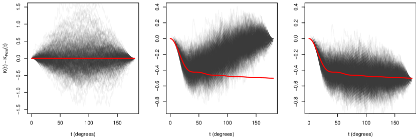
Figure 2: Each panel shows $\hat{K}(t)-K_{\textup{Pois}}(t)$ for 500 simulated point patterns on $S^{2}$ with 25 points on average together with the theoretical value of $K(t)-K_{\textup{Pois}}(t)$ for the model (red line). Left: Poisson model and usual non-parametric estimator (3.7). Middle: Most repulsive DPP and usual non-parametric estimator (3.7). Right: Most repulsive DPP and modified non-parametric estimator (3.10).

Figure 2 illustrates the potential bias for a most repulsive DPP with 25 points (the low number of points helps to emphasize the bias since the error in this case is $1/\rho=1/(25/(4\pi))\approx 0.5$). Each panel shows the difference between a non-parametric estimate of $K$ and the theoretical value for a Poisson process $K_{\textup{Pois}}$ based on 500 simulated point patterns on $S^{2}$ under the DPP model. For reference the left panel shows the perfectly unbiased result obtained when simulating a Poisson process with 25 points on average and using (3.7) to estimate $K$. The middle panel shows the bias when (3.7) is used in the case of a most repulsive DPP with 25 points. The right panel shows how the bias is removed if (3.10) is used instead.

In the case of a DPP the bias problem of the non-parametric estimator for large distances is best illustrated in the somewhat special case of very low intensity, but we believe the critique and bias problem remains valid for many other model classes. In particular we expect that models for clustering may attain values of $K(\pi)$ much larger than $4\pi$ and suffer from much larger bias, but it is left as an open problem to investigate this further.

4 DPPs on the sphere

We start in Section 4.1 with the definition of a DPP on $\mathbb{S}^{2}$ and discusses in Section 4.2 why a DPP produces regular point patterns, while the more technical details on existence of a DPP and its density function with respect to a unit rate Poisson process are deferred to Appendix B. Then in Section 4.3 we characterize isotropic DPPs and consider parametric models for their kernels. Functional summary statistics for such models are discussed in Section 4.4. Finally, in Section 4.5 we construct anisotropic DPPs.

4.1 Definition and assumptions

Consider again a simple finite point process $\bm{X}$ on $\mathbb{S}^{2}$. For a given complex function $C$ defined on the product space $\mathbb{S}^{2}\times\mathbb{S}^{2}$, we say that $\bm{X}$ is a DPP if it has joint intensities of any order $n=1,2,\ldots$ which can be expressed in terms of certain determinants with entries specified by $C$ as detailed below. An alternative specification in terms of the density for a DPP is given in Appendix B.2, while Appendix B.1 discusses the technical conditions for the existence of a DPP.

Definition. $\bm{X}$ is a DPP with kernel $C$ if for all $n=1,2,\ldots$ and all $\bm{x}_{1},\ldots,\bm{x}_{n}\in\mathbb{S}^{2}$,

$$\rho^{(n)}(\bm{x}_{1},\ldots,\bm{x}_{n})=\det\left(C(\bm{x}_{i},\bm{x}_{j})_{i,j=1,\ldots,n}\right)$$ (4.1)

where $\det\left(C(\bm{x}_{i},\bm{x}_{j})_{i,j=1,\ldots,n}\right)$ is the determinant of the $n\times n$ matrix with $(i,j)$th entry $C(\bm{x}_{i},\bm{x}_{j})$. Then we write $\bm{X}\sim\mathrm{DPP}(C)$.

Notice the following when $\bm{X}\sim\mathrm{DPP}(C)$. The intensity function is the diagonal of the kernel:

$$\rho(\bm{x})=C(\bm{x},\bm{x}),\qquad\text{$\bm{x}\in\mathbb{S}^{2}$}.$$

The expected number of points is the trace of the kernel:

$$\eta:=\mathrm{E}\left[N\left(\mathbb{S}^{2}\right)\right]=\int C(\bm{x},\bm{x})\,\mathrm{d}\nu(\bm{x}).$$ (4.2)

A Poisson process on $\mathbb{S}^{2}$ with intensity function $\rho$ is the special case of a DPP where $C(\bm{x},\bm{x})=\rho(\bm{x})$ for $\bm{x}\in\mathbb{S}^{2}$, and $C(\bm{x},\bm{y})=0$ for $\bm{x}\neq\bm{y}$. Moreover, it follows from (4.1) and since $\rho^{(n)}$ is non-negative that $C$ has to be positive semi-definite.

In the remainder of this paper we assume that $\bm{X}\sim\mathrm{DPP}(C)$ where as in most other works on DPPs, we restrict attention to the case where the kernel is Hermitian. In other words, $C$ is a complex covariance function. We allow the kernel to be complex, since this becomes convenient when considering simulation of DPPs, cf. [21]. However, isotropy of $C$ implies that it is real, and all specific models for covariance functions considered in this paper will be real. Notice that we have already assumed that $C$ is of finite trace class since it is required that $\eta<\infty$. Finally, we assume that $C$ is square integrable with respect to $\nu^{(2)}$.

In summary, we assume that $C$ is a square integrable complex covariance function of finite trace class. Then $\mathrm{DPP}(C)$ exists if and only if the spectrum of $C$ is bounded by 0 and 1 (for details, see Appendix B.1), in which case $\mathrm{DPP}(C)$ is unique.

4.2 Repulsiveness

By (4.1) and since $C$ is a covariance function, we have

$$\rho^{(n)}(\bm{x}_{1},\ldots,\bm{x}_{n})\leq\rho(\bm{x}_{1})\cdots\rho(\bm{x}_{n})$$

with equality only if $\bm{X}$ is a Poisson process with intensity function $\rho$. Therefore, a DPP is repulsive unless it is a Poisson process. Letting

$$R(\bm{x},\bm{y})=\frac{C(\bm{x},\bm{y})}{\sqrt{C(\bm{x},\bm{x})C(\bm{y},\bm{y})}},\qquad\text{$\bm{x},\bm{y}\in\mathbb{S}^{2}$},$$

be the correlation function corresponding to $C$ when $\rho(\bm{x})\rho(\bm{y})>0$, then

$$g(\bm{x},\bm{y})=1-|R(\bm{x},\bm{y})|^{2}\qquad\text{if $\rho(\bm{x})\rho(\bm{y})>0$}$$

and we set $g(\bm{x},\bm{y})=0$ if $\rho(\bm{x})\rho(\bm{y})=0$. Thus $g\leq 1$, again showing that a DPP is repulsive.

4.3 Isotropic/homogeneous DPPs

4.3.1 Characterization of isotropic kernels

Assume that $\bm{X}\sim\mathrm{DPP}(C)$ where the kernel is isotropic, i.e., it depends only on geodesic distance,

$$C(\bm{x},\bm{y})=C_{0}(s),\quad s=s(\bm{x},\bm{y})=\arccos(\bm{x}\cdot\bm{y}),\qquad\text{$\bm{x},\bm{y}\in\mathbb{S}^{2}$}.$$ (4.3)

Further, the assumption that $C$ is a covariance function implies that $C_{0}$ is a real function defined on $[0,\pi]$ such that $C$ is positive semi-definite. We follow [7] in calling $C_{0}$ the radial part of $C$, and we slightly abuse notation and write $\bm{X}\sim\mathrm{DPP}(C_{0})$.

Clearly, $\bm{X}$ is then an isotropic/homogeneous DPP. In particular any point in $\bm{X}$ is uniformly distributed on $\mathbb{S}^{2}$, the intensity $\rho=C_{0}(0)$ is constant and equal to the maximal value of $C_{0}$, and $\eta=4\pi\rho$ is the expected number of points in $\bm{X}$.

In the sequel, assume that $\rho>0$ (otherwise $\bm{X}=\emptyset$). Then

$$R_{0}(s)=C_{0}(s)/\rho$$ (4.4)

is the radial part of the correlation function $R$ associated to $C$. The allowed range of $\rho$ in terms of $R_{0}$ is the interval from 0 to

$$\rho_{\max}(R_{0})=1/\|R\|$$ (4.5)

where $\|R\|<\infty$ denotes the largest eigenvalue of $R$ (see Appendix B.1 and Appendix B.3). Furthermore, the pair correlation function is isotropic and given by

$$g(\bm{x},\bm{y})=g_{0}(s)=1-R_{0}(s)^{2}.$$ (4.6)

This implies that $g_{0}(0)=0$ (however, in case of a Poisson process, it is custom to set $g_{0}(0)=1$, since $\rho^{(2)}(\bm{x},\bm{y})=\rho^{2}$ for $\nu^{(2)}$ almost all $(\bm{x},\bm{y})\in\mathbb{S}^{2}\times\mathbb{S}^{2}$).

Now, assume that $C_{0}$ is continuous. Then, by a classical result of [33], $C_{0}$ being the radial part of a continuous isotropic covariance function $C$ is equivalent to assume that

$$C_{0}(s)=\sum_{\ell=0}^{\infty}\frac{2\ell+1}{4\pi}\alpha_{\ell}P_{\ell}(\cos s),\qquad\text{$s\in[0,\pi]$},$$ (4.7)

where each $\alpha_{\ell}\geq 0$ is an eigenvalue, $\sum_{\ell=0}^{\infty}(2\ell+1)\alpha_{\ell}<\infty$, and

$$P_{\ell}(x)=\frac{1}{2^{\ell}\ell!}\frac{\mathrm{d}^{\ell}}{\mathrm{d}x^{\ell}}\{(x^{2}-1)^{\ell}\},\qquad\text{$-1<x<1$},$$ (4.8)

is the Legendre polynomial of degree $\ell=0,1,\ldots$ (see p. 167 in [28]). The eigenvalues $\alpha_{\ell}$ are also called Mercer coefficients and the collection of Mercer coefficients is the spectrum of the kernel $C$ (see Appendix B.1 and Appendix B.3). Note that

$$R_{0}(s)=\sum_{\ell=0}^{\infty}\beta_{\ell}P_{\ell}(\cos s),\qquad\text{$s\in[0,\pi]$},$$

where

$$\beta_{\ell}=(2\ell+1)\alpha_{\ell}/\eta,\qquad\text{$\ell=0,1,\ldots,$}$$

is a discrete probability distribution, cf. (4.4) and (4.7). Conversely, given a continuous correlation function $R_{0}$, i.e., given the sequence $\beta_{0},\beta_{1},\ldots$, (4.5) gives the upper bound on the expected number of points:

$$\eta_{\max}(R_{0})=\inf\{(2\ell+1)/\beta_{\ell}:\ell=0,1,\ldots\}.$$

In [21] we quantify both global and local repulsiveness in terms of the pair correlation function when the intensity is fixed, and we point out that there is a trade-off between intensity and the degree of repulsiveness. Loosely speaking the degree of repulsiveness increases as the spectrum of $C$ tends to a step function which for small indices $\ell$ is one and for larger indices $\ell$ is zero. Therefore, for any integer $m\geq 0$, we refer to a DPP with kernel (B.4) such that $\alpha_{\ell}=1$ for $\ell\leq m$ and $\alpha_{\ell}=0$ for $\ell>m$ as the most repulsive (isotropic) DPP with $\eta=(m+1)^{2}$ (since in this case $\eta=\sum_{\ell=0}^{m}(2\ell+1)=(m+1)^{2}$; see [21] for a definition when $\eta$ is any positive number). The Poisson process is another extreme obtained when the spectrum tends to zero (but $\rho$ is still fixed). The right panel of Figure 1 shows a realization of the most repulsive DPP when $\eta=15^{2}=225$.

4.3.2 Examples

Consider the multiquadric family [9] given by

$$C_{0}=\rho R_{0},\quad R_{0}(s)=\frac{(1-\delta)^{2\tau}}{(1+\delta^{2}-2\delta\cos s)^{\tau}},\quad\text{$0<\rho\leq\rho_{\max}(R_{0})$, $\tau>0$, $0<\delta<1$}.$$

As detailed in [21], the eigenvalues $\alpha_{\ell}$ can easily be calculated numerically, which makes it possible to simulate realizations from this model. In Section 4.4 below we furthermore derive a closed form expression for the $K$-function for the model, which we will use for statistical tests, and in future work it can also be used for parameter estimation (as discussed later in Section 5). In [21] we show that the model is quite flexible and covers the range from no to intermediate repulsiveness, but in general it does not cover the most repulsive DPP (only when the expected number of points is very low). The middle panel of Figure 1 shows a realization of a multiquadric model where first we fixed $\eta=225$ and $\tau=10$, and then $\delta=0.68$ was chosen as the smallest value such that the model is well-defined. For practical purposes this corresponds to the most repulsive multiquadric model (the degree of repulsiveness grows as $\tau$ grows and $\delta$ decreases). For comparison a realization of a Poisson process with $\eta=225$ is shown in the left panel, and it is easy to visually confirm that the multiquadric model has a higher degree of repulsiveness than the Poisson process.

In the special case of $\tau=1/2$ we obtain the inverse multiquadric family where $\beta_{\ell}=\delta^{\ell}(1-\delta)$ specifies a geometric distribution and

$$\alpha_{\ell}=\eta{\delta^{\ell}(1-\delta)}/{(2\ell+1)},\quad\eta_{\max}(R_{0})={1}/{(1-\delta)}.$$

To notice the trade-off between the intensity and the degree of repulsiveness, observe that $\eta_{\max}(R_{0})$ is a strictly increasing function of $\delta$ with range $(1,\infty)$, while since $R_{0}(s)$ with $s\not=0$ is a strictly decreasing function of $\delta$, the DPP becomes less repulsive as $\delta$ increases. In the limit as $\delta\rightarrow 1$ we obtain $R_{0}(s)=0$ corresponding to a Poisson process; notice that $\alpha_{\ell}\rightarrow 0$ for $\ell=0,1,\ldots$ On the other hand, as $\delta\rightarrow 0$ and if $\eta=\eta_{\max}(R_{0})$ we obtain the most repulsive DPP but with the mean number of points only equal to 1. As demonstrated in [21], even for $\eta=10$ the DPP is rather far away from the most repulsive DPP, and for $\eta=100$ it is rather close to a Poisson process. So the inverse multiquadric family may be of limited interest except for theoretical considerations.

For the inverse multiquadric model both the kernel and the Mercer coefficients are expressible on closed form, while in the general multiquadric model the Mercer coefficients lend themselves to relatively simple numerical evaluation. This is a rather unique case, and in [21] we consider a number of other models and conclude that the most useful approach for obtaining flexible parametric models that cover the full range of possible repulsiveness for DPPs is a direct modelling of the spectrum. One example of a flexible model is the case

$$\alpha_{\ell}=\frac{1}{1+\beta\exp\left((\ell/\alpha)^{\kappa}\right)}\,,\qquad\text{$\ell=0,1,\ldots,$}$$

where $\alpha>0$, $\beta>0$, and $\kappa>0$ are parameters. Since all $\alpha_{\ell}\in(0,1)$, the DPP is well defined and has a density specified by (B.2), while $\eta$ may be evaluated by numerical methods. As demonstrated in [21], the model covers a wide range of repulsive DPPs, including any homogeneous Poisson process and any most repulsive DPP.

4.4 Functional summary statistics for isotropic DPPs

Let $\bm{X}$ be an isotropic DPP with an explicit model for the kernel $C_{0}(s)=\rho R_{0}(s)$. Then the pair correlation function is given by (4.6) and the $K$-function is given by (3.8). In particular for the multiquadric model of Section 4.3.2 we can easily derive a closed-form expression for the $K$-function using integration by substitution:

$$K_{\textup{mq}}(s)=K_{\textup{Pois}}(s)-2\pi\frac{(1+\delta)(1-\delta)}{2\delta(1-2\tau)}\Bigl{(}\left(\frac{1+\delta^{2}-2\delta}{1+\delta^{2}-2\delta\cos(s)}\right)^{2\tau-1}-1\Bigr{)},\quad\text{$\tau\neq 1/2$},$$ (4.9)

while for the inverse multiquadric family we get

$$K_{\textup{imq}}(s)=K_{\textup{Pois}}(s)-2\pi\frac{(1+\delta)(1-\delta)}{2\delta}\ln\left(\frac{1+\delta^{2}-2\delta\cos(s)}{1+\delta^{2}-2\delta}\right),\quad\text{$\tau=1/2$}.$$ (4.10)

The formulae (4.9)-(4.10) also hold for the inhomogeneous $K$-function when $X$ is a correlation isotropic DPP obtained by independent thinning of an isotropic DPP with multiquadric kernel.

For DPP models where we have explicit expressions for the Mercer coefficients but not for the kernel, we can use (4.6)-(4.7) to calculate $g_{0}$ numerically, and then use numerical integration to calculate the $K$-function, cf. (3.8). For instance, this approach has to be used both for the flexible model mentioned in Section 4.3.2 and for the most repulsive DPP, and it was used to produce the theoretical (red) curve in the middle and right panels of Figure 2.

The three point patterns in Figure 1 are realizations of DPPs with different degrees of repulsiveness: From left to right, there is none (Poisson DPP), intermediate (multiquadric DPP), and strong (most repulsive DPP) interaction. In the following we will discuss the corresponding non-parametric estimates of $K$ and $G$ and to what extend these can be used to discriminate between the three cases.

Figure 3 shows the non-parametric estimates of $K$ and $G$ for all three patterns along with the theoretical curve for a Poisson process, and as expected the estimates generally have smaller values for the more repulsive models. To produce this figure with the developed software, e.g. for the multiquadric DPP, we simulate a realization of the model and estimate $K$ by using the following commands:

  mqmodel <- dppMQ(lambda = 225/(4*pi), delta = 0.68, tau = 10)
  Xmq     <- simulate(mqmodel)
  Kmq     <- Ksphere(Xmq, rmax = 10, angle = TRUE)
  plot(Kmq)

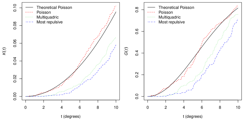
Figure 3: Non-parametric estimates of $K$ (left) and $G$ (right) for the three point patterns in Figure 1 and the theoretical curves for a Poisson process as reference. The abscissa is the angle in degrees between pairs of points on the sphere.

A simple way to assess the difference between the summary statistics is to use pointwise envelopes simulated under the null model, which is a technique with a long history for point patterns in Euclidean space (see e.g. [2] for an accessible account). For example, in order to generate pointwise envelopes for the $K$-function, with significance level 1% for the realization of a multiquadric DPP generated above under a Poisson null model, and plot the results (not shown here), we use the commands

  envmq <- envelope(Xmq, Ksphere, nsim = 199)
  plot(envmq)

This means that if we fix a distance a priori and reject the null hypothesis if the non-parametric estimate of the summary statistic for the data is outside the envelopes at this distance, then this is a test with significance level 1%. However, the main drawback is that in practice it is very hard to only do a pointwise test when the envelopes show the test results at many scales at once. This problem has been well-known for decades and a recent account can be found in Chapter 10 of [2]. As an alternative to this approach so-called rank count envelopes were developed in [26] which have an interpretation as a global test, while still providing a graphical output that can be used to infer the spatial scales where the data significantly deviates from the null model. An extra advantage of this approach is that several functional summary statistics can be combined in one test to give an overall correct significance level and thereby avoid any multiple testing problems. This test was performed on the $K$- and $G$-function simultaneously for the multiquadric point pattern with a Poisson null model which based on 2499 simulations yielded a highly significant $p$-value of 0.0004, which is the lowest possible $p$-value based on 2500 summary functions (2499 simulated and 1 data). The corresponding graphical test is shown in Figure 4, where we have separated the values related to $K$ and $G$ into separate plots even though the calculation of the envelopes are based on concatenating the values of $K$ and $G$ into one long vector. Notice that more significant departures from the null model are detected by the $K$-function which appears to provide a more powerful test in this case (and in our experience this also applies to the other examples in this paper). While it is useful to know the spatial scales leading to rejection of the null hypothesis, we should be very cautious when interpreting the $K$-function due to the cumulative nature of the function, cf. Section 3.2.

Figure 4: Simultaneous rank count envelopes for $K$ (left) and $G$ (right) for the multiquadric point pattern in the middle panel of Figure 1 based on 2499 simulations from the Poisson null model. Filled circles on the abscissa correspond to distances (in terms of angles in degrees) where the data curve exits the envelopes indicating significant departure from the Poisson null model.

If we use the same test against the most repulsive DPP as the null model based on 999 simulations, the $p$-value is 0.001 (which is the lowest possible value based on 1000 summary functions). Finally, if we test the most repulsive pattern (right panel in Figure 1) against the multiquadric DPP model with $\eta=225$, $\delta=0.68$, and $\tau=10$, we get a $p$-value of $0.008$. If instead we use $K$ respective $G$ only for the rank count test, we obtain a $p$-value of $0.005$ respective $0.106$, which again indicates that $K$ is the more powerful of the two.

4.5 Models constructed by thinning an isotropic DPP

This section focuses on anisotropic/inhomogeneous DPP $\bm{X}$ constructed by independent thinning of an isotropic/homogeneous DPP $\bm{Y}$ on $\mathbb{S}^{2}$ with kernel $C_{Y}$ and $n$th order product intensity $\rho^{(n)}_{Y}$. We also follow [16] in considering a doubly stochastic construction where $\bm{X}$ is obtained by a dependent thinning of $\bm{Y}$. Thereby we can model regularity on the small scale and clustering on the large scale.

Suppose

$$\bm{X}=\{\bm{x}\in\bm{Y}:\Pi(\bm{x})\geq U(\bm{x})\}$$

where $\bm{\Pi}=\{\Pi(\bm{x}):\bm{x}\in\mathbb{S}^{2}\}$ is a random process of ‘selection probabilities’ $\Pi(\bm{x})$, $\bm{U}=\{U(\bm{x}):\bm{x}\in\mathbb{S}^{2}\}$ is a process of mutually independent random variables $U(\bm{x})$ which are uniformly distributed on $[0,1]$, and $\bm{Y},\bm{\Pi},\bm{U}$ are mutually independent. If $\bm{\Pi}$ is deterministic, then $\bm{X}$ is an independent thinning of $\bm{Y}$, having $n$th order product intensity

$$\rho^{(n)}_{X}(\bm{x}_{1},\ldots,\bm{x}_{n})=\Pi(\bm{x}_{1})\cdots\Pi(\bm{x}_{n})\rho^{(n)}_{Y}(\bm{x}_{1},\ldots,\bm{x}_{n})$$

and so $\bm{X}$ is seen to be a DPP with kernel

$$C_{X}(\bm{x},\bm{y})=\Pi(\bm{x})\Pi(\bm{y})C_{Y}(\bm{x},\bm{y}).$$

This DPP is anisotropic if $\Pi$ is not constant. If $\bm{\Pi}$ is random, then in general $\bm{X}$ is a dependent thinning of $\bm{Y}$, with

$$\rho^{(n)}_{X}(\bm{x}_{1},\ldots,\bm{x}_{n})=\mathrm{E}\left[\Pi(\bm{x}_{1})\cdots\Pi(\bm{x}_{n})\right]\rho^{(n)}_{Y}(\bm{x}_{1},\ldots,\bm{x}_{n})$$

and we cannot conclude that $\bm{X}$ is a DPP unless the selection probabilities are independent.

Figure 5: Pair correlation functions for $\Pi$-thinnings of a most repulsive DPP with 400 points (see Figure 6 for a realization). In all panels the covariance function for the underlying Gaussian process is multiquadric with variance $\kappa=8$, while $\tau=0.25,1,10$ from left to right panel, and $\delta=0.5,0.7,0.8,0.85$ from top to bottom curve within each panel.

In particular assume that $\bm{Y}$ is homogeneous with intensity $\rho_{Y}$ and pair correlation function $g_{0,Y}(s)$, and the distribution of $\bm{\Pi}$ is invariant under the action of $\mathcal{O}(3)$ on $\mathbb{S}^{2}$. Then $\bm{X}$ is homogeneous, with intensity and pair correlation function

$$\rho_{X}=q\rho_{Y},\qquad g_{X,0}(s)=M_{0}(s)g_{Y,0}(s),\qquad\text{$s\in[0,\pi]$},$$

where $q=\mathrm{E}[\Pi(\bm{x})]$ is the mean selection probability and, setting $0/0=0$,

$$M_{0}(s)=M(\bm{x},\bm{y})=\frac{\mathrm{E}[\Pi(\bm{x})\Pi(\bm{y})]}{\mathrm{E}[\Pi(\bm{x})]\mathrm{E}[\Pi(\bm{y})]},\qquad\text{$\bm{x},\bm{y}\in\mathbb{S}^{2}$},$$

depends only on $s=s(\bm{x},\bm{y})$. For instance, assume that $-\log\bm{\Pi}$ is the $\chi^{2}$-process given by

$$\Pi(\bm{x})=\exp\left(-\bm{Z}(\bm{x})^{2}/2\right),\qquad\text{$\bm{x}\in\mathbb{S}^{2}$},$$ (4.11)

where $\bm{Z}$ is a zero-mean Gaussian process with isotropic covariance function $K$. Denoting $K_{0}$ the radial part of $K$ and assuming the variance $\kappa=K_{0}(0)$ is positive, we have the same formulas as obtained in [16] but for point processes on $\mathbb{R}^{d}$:

$$q=(1+\kappa)^{-1/2},\quad M_{0}(s)=\left[1-\frac{R_{0}(s)^{2}}{(1+1/\kappa)^{2}}\right]^{-1/2},$$

where $R_{0}=K_{0}/\kappa$ is the (radial part of the) correlation function of $\bm{Z}$. Note that $g_{Y,0}\leq 1$ while $M_{0}(s)\geq 1$ is typically a decreasing function of $s$. In fact it is possible to obtain that $g_{X,0}(s)\leq 1$ for small values of $s$ and $g_{X,0}(s)\geq 1$ for large values of $s$, reflecting regularity on the small scale and clustering on the large scale.

This is illustrated in Figure 5, where the original process $\bm{Y}$ is a most repulsive DPP with 400 points and the underlying Gaussian process $\bm{Z}$ has a multiquadric covariance function with variance $\kappa=8$ such that the mean selection probability is $q=1/3$. Thus the expected number of points of the thinned process $\bm{X}$ is $400/3$. As can be seen from the figure, both $\tau$ and $\delta$ influence the range of the positive association between points on the longer scale: For both parameters smaller values yield long range dependence while the dependence dies out quicker for larger values. Similar figures (not shown here) show that changing the original DPP to a multiquadric model effectively shifts the curves such that the value of $s$ where $g_{X,0}(s)$ crosses the Poisson reference value 1 shifts to the left, which is to be expected since the original DPP is less repulsive in this case. Note that the geodesic distance in this and subsequent figures is given in terms of the angle between points on the sphere measured in degrees from 0 to 180 (as we expect the reader to relate more easily to these than distances which are effectively in radians).

Note that simulation of $\bm{Z}$ is easy, if we assume that $K$ has a Mercer representation as in (B.4), with eigenvalues $\alpha_{\ell}^{Z}$. Then we generate independent standard normally distributed random variables $W_{\ell,k}^{(1)}$ and $W_{\ell,k}^{(2)}$ for $\ell=0,1,\ldots$ and $k=-\ell,\ldots,\ell$, and observe that

$$\sum_{\ell=0}^{\infty}\sqrt{\alpha_{\ell}^{Z}}\sum_{k=-\ell}^{\ell}\left\{W_{\ell,k}^{(1)}\mathrm{Re}\left[Y_{\ell,k}(\bm{x})\right]+W_{\ell,k}^{(2)}\mathrm{Im}\left[Y_{\ell,k}(\bm{x})\right]\right\},\qquad\text{$\bm{x}\in\mathbb{S}^{2}$},$$ (4.12)

is a zero-mean Gaussian process with covariance function $K$ (this follows from a straightforward calculation, using (B.4) and the fact that $K$ is real). In practice a truncation of the infinite series in (4.12) has to be used. From (4.7) we have $\kappa=K_{0}(0)=\sum_{0}^{\infty}\alpha_{\ell}^{Z}(2\ell+1)/(4\pi)$, and we choose the truncation such that the truncated series equals 99% of the given value of $\kappa$. Figure 6 shows a realization of the original unthinned DPP $\bm{Y}$ while Figure 7 shows the result after $\Pi$-thinning.

Figure 6: Northern and Southern Hemispheres of a most repulsive DPP with 400 points used as the original process $Y$ before $\Pi$-thinning (see text). The hemispheres are projected to unit discs with an equal-area azimuthal projection.

Figure 7: Northern and Southern Hemispheres of a $\Pi$-thinning of the most repulsive DPP with 400 points shown in Figure 6. The Gaussian process underlying the $\Pi$-thinning has multiquadric covariance function with $\kappa=8$, $\tau=1$, and $\delta=0.5$. The hemispheres are projected to unit discs with an equal-area azimuthal projection and the pattern contains 148 points in total.

Finally, we notice another construction, namely by applying a one-to-one smooth transformation $\mathbb{S}^{2}\mapsto\mathbb{S}^{2}$ on $\bm{Y}$ to obtain $\bm{X}$. This results again in that $\bm{X}$ is a DPP with a kernel that can be specified in terms of $C_{Y}$ and the derivative of the transformation. We skip the details here, but see [14, 15] for the result in the case of transformed DPPs on $\mathbb{R}^{d}$.

5 Discussion

In Section 3.2, for a second order intensity reweighted isotropic point process on the sphere, we provided non-parametric estimates of the $F$, $G$ and $K$-functions. In the literature for point processes defined on Euclidean spaces there is considerable discussion of edge correction factors, which account for the edge effects that arise when estimating functional summary statistics near the boundaries of an observation window. In Section 3.2, we exemplified this only in the case when the process is fully observed or when minus sampling is used, while [17] provide further edge correction factors. In the planar case [2] mentions that “So long as some kind of edge correction is performed …, the particular choice of edge correction technique is usually not critical.” We expect the situation to be similar for point patterns on the sphere.

Our paper started with a brief discussion on how to model aggregation or regularity for point processes on the two-dimensional sphere or more generally on $\mathbb{S}^{d}$, where two examples are the Thomas process and DPPs. Regarding regularity this may be caused by repulsiveness between the points or by some thinning mechanism as specified in the following list of models, usually defined on $\mathbb{R}^{d}$ but straightforwardly adapted to $\mathbb{S}^{d}$:

• Matérn hard core processes of types I-III can be simulated by their constructions as dependent thinnings of Poisson processes, see [11, 19, 20, 35]. However, for the types I-II, the moments of the process will be tractable while the likelihood (density) will be intractable; and for type III, the opposite is the case.

• Simple sequential inhibition and other hard sphere packing models (as reviewed in [3, 12]) can be simulated by their simple constructions of points added one by one, but otherwise they are hard to analyse.

• Gibbs point processes offer much more flexibility for modelling inhibition or repulsiveness, but their simulation may be time-consuming and neither the moments nor the likelihood are tractable, see [24, 25] and the references therein.

As noticed, DPPs are in many ways more attractive than these models, since DPPs can be easily simulated and their joint intensities and likelihood are tractable. In comparison with DPPs on $\mathbb{R}^{d}$, DPPs on $\mathbb{S}^{d}$ are in many ways easier to handle, since they are defined on a compact set and we can more easily deal with the Mercer representation, at least in the isotropic case.

We have considered examples of simulated point patterns on the sphere under various DPP models. Indeed it would be interesting to analyze real point pattern data sets on the sphere using parametric DPP models. Here we expect that inhomogeneous/anisotropic DPPs will be of more relevance than homogeneous/isotropic DPPs. As in [14, 15] parameter estimation may be done by either maximum likelihood or a composite likelihood or minimum contrast method based on the intensity and pair correlation functions. In [14, 15] we noticed that the latter methods work quite well in comparison with maximum likelihood.

Other point process models than DPPs on the sphere may of course be of relevance for applications. For instance, the spectral representation (B.1) allows us to construct and simulate Gaussian processes, cf. (4.12). Thus we can also deal with log Gaussian Cox processes (LGCPs) on the sphere, where all the statistical methodology for LGCPs on Euclidean spaces [23, 24, 25] can be easily adapted to the sphere.

Finally, we notice that space-time point process models on the sphere, whether being DPPs or LGCPs or of another type, might be worth studying, where of course the direction of time should be taken into consideration.

Acknowledgment

Supported by the Danish Council for Independent Research | Natural Sciences, grant 12-124675, “Mathematical and Statistical Analysis of Spatial Data”, and by the “Centre for Stochastic Geometry and Advanced Bioimaging”, funded by grant 8721 from the Villum Foundation. We are grateful to Markus Kiderlen for providing Appendix A.

Appendix A Relation between Palm distributions

For Borel sets $A\subseteq\mathbb{S}^{2}$ and a fixed event $F\in\mathcal{F}$, denote $\mu_{F}(A)$ the expected value in the right side of (3.2), i.e.,

$$\mu_{F}(A)=\mathrm{E}\sum_{\bm{x}\in\bm{X}\cap A}1\left[R_{\bm{x}}^{\top}(\bm{X}\setminus\{\bm{x}\})\in F\right].$$

This is a measure on the Borel sets contained in $\mathbb{S}^{2}$, and as verified in Section 3.1 it is rotation invariant if the distribution of $\bm{X}$ is absolutely continuous with respect to the unit rate Poisson process (or any other isotropic Poisson process) on $\mathbb{S}^{2}$. However, let $\mathbf{e}_{1},\mathbf{e}_{2},\mathbf{e}_{3}$ be the standard basis in $\mathbb{R}^{3}$ (so $\mathbf{e}_{3}=\mathbf{e}$) and consider the point process $\bm{Z}=\mathcal{O}\{\mathbf{e}_{1},\mathbf{e}_{2}\}$ where $\mathcal{O}$ is a uniform rotation (i.e., it follows the normalized Haar measure on $SO(3)$). Obviously, the distribution $\bm{Z}$ is not absolutely continuous with respect to the unit rate Poisson. Further, for $\epsilon>0$ and $\bm{x}\in\mathbb{S}^{2}$, denote $A_{\epsilon}(\bm{x})=\{\bm{y}\in\mathbb{S}^{2}:s(\bm{x},\bm{y})<\epsilon\}$ and let $F$ be the set of all finite subsets of $\mathbb{S}^{2}$ with at least one point in $A_{2\epsilon}(-\mathbf{e}_{2})$. Then, for $A=A_{\epsilon}(\mathbf{e}_{1})\cup A_{\epsilon}(\mathbf{e}_{2})$, $A^{\prime}=A_{\epsilon}(\mathbf{e}_{2})\cup A_{\epsilon}(\mathbf{e}_{3})$, and sufficiently small $\epsilon$, it follows straightforwardly that $A^{\prime}$ is a rotation of $A$, $\mu_{F}(A)=0$, and $\mu_{F}(A^{\prime})>0$. Consequently, $\mu_{F}$ is not in general rotation invariant, and we need a more complicated construction of the reduced Palm distribution at $\mathbf{e}$: Let $\theta$ be uniform in $[0,2\pi)$ and denote $\mathcal{O}_{\theta}$ the rotation with angle $\theta$ around $\mathbf{e}$ as the axis of the rotation. Suppose $\theta$ and $\bm{X}$ are independent. It can be shown that for any fixed $F\in\mathcal{F}$,

$$\chi_{F}(A)=\mathrm{E}\sum_{\bm{x}\in\bm{X}\cap A}1[\mathcal{O}_{\theta}R_{\bm{x}}^{\top}(\bm{X}\setminus\{\bm{x}\})\in F]$$

is a rotation invariant measure, and $\mathcal{O}_{\theta}R_{\bm{x}}^{\top}$ follows the distribution of a uniform rotation given that it maps $\bm{x}$ to $\mathbf{e}$. Finally, it follows from a straightforward calculation that $\bm{X}^{!}_{\bm{x}}$ is distributed as $R_{\bm{x}}\mathcal{O}_{\theta}^{\top}\bm{X}^{!}_{\mathbf{e}}$, where $\mathrm{P}\left(\bm{X}^{!}_{\mathbf{e}}\in F\right)=\chi_{F}(A)/[\rho\nu(A)]$ for an arbitrary Borel set $A\subseteq\mathbb{S}^{2}$ with $\nu(A)>0$.

Appendix B Further results for DPPs

B.1 Existence

Recall that the kernel $C$ is assumed to be a complex covariance function of finite trace class and is square integrable. By [10, Lemma 4.2.6 and Theorem 4.5.5] $\mathrm{DPP}(C)$ exists if and only if the spectrum of $C$ is bounded by 0 and 1, and then $\mathrm{DPP}(C)$ is unique. Below we explain what the spectrum is.

Consider a covariance function $K:\mathbb{S}^{2}\times\mathbb{S}^{2}\mapsto\mathbb{C}$ which is of finite trace class and is square integrable. Then, by Mercer’s theorem (e.g. [29, Section 98]) and [10, Lemma 4.2.2]), ignoring a $\nu^{(2)}$-nullset, $K$ has a spectral representation

$$K(\bm{x},\bm{y})=\sum_{n=1}^{\infty}\alpha_{n}Y_{n}(\bm{x})\overline{Y_{n}(\bm{y})},\qquad\text{$\bm{x},\bm{y}\in\mathbb{S}^{2}$}$$ (B.1)

where $Y_{1},Y_{2},\ldots$ are eigenfunctions which form an orthonormal basis for the space of square integrable complex functions with respect to $\nu$. We call (B.1) the Mercer representation of $K$, the eigenvalues $\alpha_{i}$ for the Mercer coefficients, and $\operatorname{spec}(K)=\{\alpha_{1},\alpha_{2},\ldots\}$ the spectrum of $K$.

When $\bm{X}\sim\mathrm{DPP}(C)$, we denote the Mercer coefficients of $C$ by $\lambda_{1},\lambda_{2},\ldots$, and to ensure existence we require that $\operatorname{spec}(C)\subset[0,1]$. Then, by (4.2) and (B.1), the mean number of points is $\eta=\sum_{n=1}^{\infty}\lambda_{n}$.

B.2 Likelihood

Suppose $\bm{X}\sim\mathrm{DPP}(C)$ where $\operatorname{spec}(C)\subset[0,1)$. Then we can work with the likelihood/density as given below.

Let $\tilde{C}:\mathbb{S}^{2}\times\mathbb{S}^{2}\mapsto\mathbb{C}$ be the complex covariance function with a Mercer representation sharing the same eigenfunctions as $C$ but with Mercer coefficients

$$\tilde{\lambda}_{n}=\frac{\lambda_{n}}{1-\lambda_{n}},\qquad\text{$n=1,2,\ldots$}.$$

Define

$$D=\sum_{n=1}^{\infty}\log\bigl{(}1+\tilde{\lambda}_{n}\bigr{)}.$$

Then, by [34, Theorem 1.5], $\mathrm{DPP}(C)$ is absolutely continuous with respect to the unit rate Poisson process (i.e., the Poisson process on $\mathbb{S}^{2}$ with intensity measure $\nu$) and has density

$$f(\{\bm{x}_{1},\ldots,\bm{x}_{n}\})=\exp(4\pi-D)\det\bigl{(}\tilde{C}(\bm{x}_{i},\bm{x}_{j})_{i,j=1,\ldots,n}\bigr{)},$$ (B.2)

for any point configuration $\{\bm{x}_{1},\ldots,\bm{x}_{n}\}\subset\mathbb{S}^{2}$, $n=0,1,\ldots$. When $n=0$ we consider the empty point configuration $\emptyset$, so $\exp(-D)$ is the probability that $\bm{X}=\emptyset$ (since $\exp(-4\pi)$ is the probability that the unit rate Poisson process is empty).

Since

$$\lambda_{n}=\frac{\tilde{\lambda}_{n}}{1+\tilde{\lambda}_{n}},\qquad\text{$n=1,2,\ldots$},$$ (B.3)

there is a one-to-one correspondence between $C$ and $\tilde{C}$. Thus, in order to construct a DPP we can start by specifying any complex covariance function $\tilde{C}$ which is of finite trace class and is square integrable. Its density is then given by (B.2), and $C$ is determined by the Mercer representation of $\tilde{C}$ and by (B.3). Then $\operatorname{spec}(C)\subset[0,1)$, and so $\mathrm{DPP}(C)$ is well-defined.

B.3 Mercer representation for an isotropic kernel

Consider the isotropic kernel $C$ in (4.3). Below we specify its Mercer representation and discusses when the corresponding DPP exists.

We need some notation. Recall (4.8) and for $k=0,\ldots,\ell$ define the associated Legendre functions $P_{\ell}^{(k)}$ and $P_{\ell}^{(-k)}$ by (see [6] p. 421)

$$P_{\ell}^{(k)}(x)=(-1)^{k}\left(1-x^{2}\right)^{k/2}\frac{\mathrm{d}^{k}}{\mathrm{d}x^{k}}P_{\ell}(x),\qquad\text{$-1\leq x\leq 1$},$$

and

$$P_{\ell}^{(-k)}=(-1)^{k}\frac{(\ell-k)!}{(\ell+k)!}P_{\ell}^{(k)}.$$

Moreover, the surface spherical harmonic functions are given by

$$Y_{\ell,k}(\bm{x})=Y_{\ell,k}(\vartheta,\varphi)=\sqrt{\frac{2\ell+1}{4\pi}\,\frac{(\ell-k)!}{(\ell+k)!}}\,P_{\ell}^{(k)}(\cos{\vartheta})\,e^{ik\varphi},\quad\text{$(\vartheta,\varphi)\in[0,\pi]\times[0,2\pi)$},$$

for $k=-\ell,\ldots,\ell$, where $\bm{x}\in\mathbb{S}^{2}$ is identified by its polar latitude and longitude $(\vartheta,\varphi)$, cf. (2.1), and where $i^{2}=-1$. In fact the surface spherical harmonic functions constitute an orthonormal basis for the space of square integrable complex functions with respect to $\nu$.

Now, by the addition formula for spherical harmonics (see [21]), (4.7) is equivalent to the Mercer representation

$$C(\bm{x}_{1},\bm{x}_{2})=\sum_{\ell=0}^{\infty}\alpha_{\ell}\sum_{k=-\ell}^{\ell}Y_{\ell,k}(\bm{x}_{1}){\overline{Y_{\ell,k}(\bm{x}_{2})}},\qquad\text{$\bm{x}_{1},\bm{x}_{2}\in\mathbb{S}^{2}$},$$ (B.4)

i.e., the Mercer coefficients are $\lambda_{\ell,k}=\alpha_{\ell}$, with $\ell=0,1,\ldots$ and $k=-\ell,\ldots,\ell$. Therefore, to ensure that $\mathrm{DPP}(C_{0})$ is well-defined, we require that the spectrum $\{\alpha_{0},\alpha_{1},\ldots\}$ is included in $[0,1]$ and that the sum

$$\sum_{\ell=0}^{\infty}(2\ell+1)\alpha_{\ell}$$

is finite, and in this case the sum is equal to $\eta$.

Similarly, if we use the alternative approach of Section B.2 where we start by specifying $\tilde{C}$: Assuming that $\tilde{C}$ is a continuous isotropic covariance function is equivalent to that

$$\tilde{C}(\bm{x}_{1},\bm{x}_{2})=\sum_{\ell=0}^{\infty}\tilde{\alpha}_{\ell}Y_{\ell,k}(\bm{x}_{1}){\overline{Y_{\ell,k}(\bm{x}_{2})}},\qquad\text{$\bm{x}_{1},\bm{x}_{2}\in\mathbb{S}^{2}$},$$ (B.5)

where all $\tilde{\alpha}_{\ell}$ are non-negative and $\sum_{\ell=0}^{\infty}(2\ell+1)\tilde{\alpha}_{\ell}<\infty$.

References

- [1] A. Baddeley, J. Møller, and R. Waagepetersen. Non- and semi-parametric estimation of interaction in inhomogeneous point patterns. Statistica Neerlandica, 54:329–350, 2000.
- [2] A. Baddeley, E. Rubak, and R. Turner. Spatial Point Patterns: Methodology and Applications with R. Chapman & Hall/CRC Press, Boca Raton, 2015.
- [3] S. N. Chiu, D. Stoyan, W. S. Kendall, and J. Mecke. Stochastic Geometry and Its Applications. Wiley, Chichester, third edition, 2013.
- [4] J.-F. Coeurjolly, J. Møller, and R. Waagepetersen. Conditioning in spatial point processes. Technical report, Centre for Stochastic Geometry and Advanced Bioimaging. Submitted for journal publication, 2015.
- [5] J.-F. Coeurjolly, J. Møller, and R. Waagepetersen. Palm distributions for log Gaussian Cox processes. Technical report, Centre for Stochastic Geometry and Advanced Bioimaging. Submitted for journal publication, 2015.
- [6] F. Dai and Y. Xu. Approximation Theory and Harmonic Analysis on Spheres and Balls. Springer Monographs in Mathematics. Springer, New York, 2013.
- [7] D. J. Daley and E. Porcu. Dimension walks through Schoenberg spectral measures. Proceedings of the American Mathematical Society, 42:1813–1824, 2013.
- [8] D. J. Daley and D. Vere-Jones. An Introduction to the Theory of Point Processes. Volume II: General Theory and Structure. Springer-Verlag, New York, second edition, 2008.
- [9] T. Gneiting. Strictly and non-strictly positive definite functions on spheres. Bernoulli, 19:1327–1349, 2013.
- [10] J. B. Hough, M. Krishnapur, Y. Peres, and B. Viràg. Zeros of Gaussian Analytic Functions and Determinantal Point Processes. American Mathematical Society, Providence, 2009.
- [11] M. L. Huber and R. L. Wolpert. Likelihood-based inference for Matérn type-III repulsive point processes. Advances in Applied Probability, 41:958–977, 2009.
- [12] J. Illian, A. Penttinen, H. Stoyan, and D. Stoyan. Statistical Analysis and Modelling of Spatial Point Patterns. John Wiley and Sons, Chichester, 2008.
- [13] G. Last. Stationary random measures on homogeneous spaces. Journal of Theoretical Probability, 23:478–497, 2010.
- [14] F. Lavancier, J. Møller, and E. Rubak. Determinantal point process models and statistical inference: Extended version. Technical report, available at arXiv:1205.4818, 2014.
- [15] F. Lavancier, J. Møller, and E. Rubak. Determinantal point process models and statistical inference. Journal of Royal Statistical Society: Series B (Statistical Methodology), 77:853–877, 2015.
- [16] F. Lavencier and J. Møller. Modelling aggregation on the large scale and regularity on the small scale in spatial point pattern datasets. Scandinavian Journal of Statistics, 2016. To appear.
- [17] T. Lawrence, A. Baddeley, R. K. Milne, and G. Nair. Point pattern analysis on a region of a sphere. Stat, 5:144–157, 2016.
- [18] M. N. M. van Lieshout and A. J. Baddeley. A nonparametric measure of spatial interaction in point patterns. Statistica Neerlandica, 50:344–361, 1996.
- [19] B. Matérn. Spatial Variation. Lecture Notes in Statistics 36, Springer-Verlag, Berlin, 1986.
- [20] J. Møller, M. L. Huber, and R. L. Wolpert. Perfect simulation and moment properties for the Matérn type III process. Stochastic Processes and their Applications, 120:2142–2158, 2010.
- [21] J. Møller, M. Nielsen, E. Porcu, and E. Rubak. Determinantal point processes on the sphere. Technical report, Centre for Stochastic Geometry and Advanced Bioimaging. Submitted for journal publication, 2015.
- [22] J. Møller and E. Rubak. Determinantal point processes and functional summary statistics on the sphere. 2016. Preprint on arxiv:1601.03448.
- [23] J. Møller, A. R. Syversveen, and R. P. Waagepetersen. Log Gaussian Cox processes. Scandinavian Journal of Statistics, 25:451–482, 1998.
- [24] J. Møller and R. P. Waagepetersen. Statistical Inference and Simulation for Spatial Point Processes. Chapman and Hall/CRC, Boca Raton, 2004.
- [25] J. Møller and R. P. Waagepetersen. Modern spatial point process modelling and inference (with discussion). Scandinavian Journal of Statistics, 34:643–711, 2007.
- [26] M. Myllymäki, T. Mrkvicka, P. Grabarnik, H. Seijo, and U. Hahn. Global envelope tests for spatial processes, 2015. Preprint on arxiv:1307.0239v4.
- [27] R Core Team. R: A Language and Environment for Statistical Computing. R Foundation for Statistical Computing, Vienna, Austria, 2015.
- [28] E. D. Rainville. Special Functions. Chelsea Publishing Co., Bronx, N.Y., first edition, 1960.
- [29] F. Riesz and B. Sz.-Nagy. Functional Analysis. Dover Publications, New York, 1990.
- [30] B. D. Ripley. The second-order analysis of stationary point processes. Journal of Applied Probability, 13:255–266, 1976.
- [31] S. M. Robeson, A. Li, and C. Huang. Point-pattern analysis on the sphere. Spatial Statistics, 10:76–86, 2014.
- [32] W. Rother and M. Zähle. Palm distributions in homogeneous spaces. Mathematische Nachrichten, 149(1):255–263, 1990.
- [33] I. J. Schoenberg. Positive definite functions on spheres. Duke Mathematical Journal, 9:96–108, 1942.
- [34] T. Shirai and Y. Takahashi. Random point fields associated with certain Fredholm determinants I: fermion, Poisson and boson point processes. Journal of Functional Analysis, 205:414–463, 2003.
- [35] J. Teichmann, F. Ballani, and K. van den Boogaart. Generalizations of Matérn’s hard-core point processes. Spatial Statistics, 3:33–53, 2013.