Nonlinear effects in buoyancy-driven variable density turbulence

Abstract

We consider the time-dependence of a hierarchy of scaled $L^{2m}$-norms $D_{m,\omega}$ and $D_{m,\theta}$ of the vorticity $\mbox{\boldmath$\omega$}=\boldsymbol{\nabla}\times\mbox{\boldmath$u$}$ and the density gradient $\boldsymbol{\nabla}\theta$, where $\theta=\log(\rho^{*}/\rho^{*}_{0})$, in a buoyancy-driven turbulent flow as simulated by Livescu & Ristorcelli (2007). $\rho^{*}(\mathbi{x},\,t)$ is the composition density of a mixture of two incompressible miscible fluids with fluid densities $\rho^{*}_{2}>\rho^{*}_{1}$ and $\rho^{*}_{0}$ is a reference normalisation density. Using data from the publicly available Johns Hopkins Turbulence Database we present evidence that the $L^{2}$-spatial average of the density gradient $\boldsymbol{\nabla}\theta$ can reach extremely large values, even in flows with low Atwood number $At=(\rho^{*}_{2}-\rho^{*}_{1})/(\rho^{*}_{2}+\rho^{*}_{1})=0.05$, implying that very strong mixing of the density field at small scales can arise in buoyancy-driven turbulence. This large growth raises the possibility that the density gradient $\boldsymbol{\nabla}\theta$ might blow up in a finite time.

1 Introduction

The irreversible mixing at a molecular level of two fluids of different densities $\rho^{*}_{2}>\rho^{*}_{1}$ is a fluid dynamical process of great fundamental interest and practical importance, especially when the fluids are turbulent. Such turbulent mixing flows occur in many different circumstances. A particularly important class arises when the buoyancy force associated with the effects of statically unstable variations in fluid density in a gravitational field actually drives both the turbulence and the ensuing mixing itself. Such flows, commonly referred to as ‘Rayleigh-Taylor instability’ (RTI) flows due to the form of the initial linear instability (Rayleigh (1900); Taylor (1950)), have been very widely studied (see Sharp (1984); Youngs (1984, 1989); Glimm et al. (2001); Dimonte et al. (2004); Dimotakis (2005); Lee et al. (2008); Hyunsun et al. (2008); Andrews & Dalziel (2010)), not least because of their relevance in astrophysics (Cabot & Cook, 2006) and fusion (Petrasso, 1994).

A key characteristic of RTI flows is that the turbulence which develops is not driven by some external forcing mechanism, but rather is supplied with kinetic energy by the conversion of ‘available’ potential energy stored in the initial density field. This kinetic energy naturally drives turbulent disorder and a cascade to small scales, with an attendant increase in the dissipation rate of kinetic energy. Such small scales also lead to ‘filamentation’, i.e. enhanced surface area of contact between the two miscible fluids and, crucially, substantially enhanced gradients in the density field, which thus also leads to irreversible mixing, and hence modification in the density distribution. There has been an explosion in interest in investigating the ‘efficiency’ of this mixing, i.e. loosely, the proportion of the converted available potential energy which leads to irreversible mixing, as opposed to viscous dissipation, (see the recent review of Tailleux (2013)), although the actual definition and calculation of the efficiency is subtle and must be performed with care – see for example Davies-Wykes & Dalziel (2014) for further discussion.

Nevertheless, there is accumulating evidence that buoyancy-driven turbulence is particularly efficient in driving mixing (Lawrie & Dalziel, 2011; Davies-Wykes & Dalziel, 2014) and certainly more efficient than externally forced turbulent flow. This evidence poses the further question whether there are some distinguishing characteristics of the buoyancy-driven turbulent flow that are different from the flow associated with an external forcing, in particular whether these characteristics can be identified as being responsible for the enhanced and efficient mixing.

The situation is further complicated by the observation that, even when the two fluids undergoing mixing are themselves incompressible, since molecular mixing generically changes the specific volume of the mixture, the velocity fields of such ‘variable density’ (VD) flows, (following the nomenclature suggested by Livescu & Ristorcelli (2007)) are in general not divergence-free. This is definitely the case when the two densities are sufficiently different such that the Boussinesq approximation may not be applied. Commonly, the Boussinesq approximation is applied when the Atwood number $At$, defined as

$$At=\frac{\rho^{*}_{2}-\rho^{*}_{1}}{\rho^{*}_{2}+\rho^{*}_{1}}\,,$$ (1)

is small ; i.e, $At\ll 1$. However, as discussed in detail in Livescu & Ristorcelli (2007), non-Boussinesq effects may occur when gradients in the density field become large. Following Cook & Dimotakis (2001) and Livescu & Ristorcelli (2007) the composition density $\rho^{*}(\mathbi{x},\,t)$ of a mixture of two constant fluid densities $\rho^{*}_{1}$ and $\rho^{*}_{2}$ ($\rho^{*}_{2}>\rho^{*}_{1}$) is expressed in dimensionless form by

$$\frac{1}{\rho^{*}(\mathbi{x},\,t)}=\frac{Y_{1}(\mathbi{x},\,t)}{\rho^{*}_{1}}+\frac{Y_{2}(\mathbi{x},\,t)}{\rho^{*}_{2}}\,,$$ (2)

where $Y_{i}(\mathbi{x},\,t)$ ($i=1,2$) are the mass fractions of the two fluids and $Y_{1}+Y_{2}=1$. (2) shows that the composition density $\rho^{*}$ is bounded by

$$\rho^{*}_{1}\leq\rho^{*}(\mathbi{x},\,t)\leq\rho^{*}_{2}\,.$$ (3)

Assuming that there is Fickian diffusion, the mass transport equations for the two species are

$$\partial_{t}\left(\rho Y_{i}\right)+\boldsymbol{\nabla}\cdot\left(\rho^{*}Y_{i}\mbox{\boldmath$u$}\right)=Pe_{0}\boldsymbol{\nabla}\cdot\left(\rho\boldsymbol{\nabla}Y_{i}\right)\,,$$ (4)

where $Pe_{0}$ is the Péclet number : the dimensionless Reynolds, Schmidt and Péclet numbers are defined in Table 1. Since the specific volume $1/\rho^{*}$ changes due to mixing, a non-zero divergence is induced in the velocity field (see Appendix A).

$$\boldsymbol{\nabla}\cdot\mbox{\boldmath$u$}=-Pe_{0}\Delta\left(\ln\rho^{*}\right)=-\frac{Pe_{0}}{\rho^{*}}\Delta\rho^{*}+\frac{Pe_{0}}{\rho^{*2}}|\boldsymbol{\nabla}\rho^{*}|^{2}\,,$$ (5)

while summing (4) over the two species yields the conventional continuity equation for mass conservation

$$\partial_{t}\rho^{*}+\boldsymbol{\nabla}\cdot\left(\rho^{*}\mbox{\boldmath$u$}\right)=0\,.$$ (6)

As discussed in Livescu & Ristorcelli (2007), the Boussinesq approximation, leading to the requirements that the velocity field is divergence-free $\boldsymbol{\nabla}\cdot\mbox{\boldmath$u$}=0$ and the mass conservation equation becomes

$$\partial_{t}\rho^{*}+\mbox{\boldmath$u$}\cdot\boldsymbol{\nabla}\rho^{*}=Pe_{0}\Delta\rho^{*}\,,$$ (7)

relies on the requirement that the second (nonlinear) term on the right hand side of (5) can be ignored compared to the first term, i.e. that

$$|\boldsymbol{\nabla}\rho^{*}|^{2}\ll\rho^{*}|\Delta\rho^{*}|\,.$$ (8)

As noted by Livescu & Ristorcelli (2007), this condition may be violated if substantial gradients develop in the density field. It is not a priori clear, even when the Atwood number is very small, that the non-divergent nature of the velocity field qualitatively changes the properties of the turbulent flow in ways which are significant to the mixing, and specifically whether regions in the flow may develop where the condition (8) is violated. This issue can be explored by careful numerical simulation, as reviewed by Livescu (2013), with a key observation (see Livescu & Ristorcelli (2007) for more details) being that the pressure distribution is substantially modified by non-Boussinesq effects.

Furthermore, the central role played by intermittency and anisotropy, as discussed in Livescu & Ristorcelli (2008) suggests that it would be instructive to focus carefully on the time-dependent evolution of nonlinearity within such buoyancy-driven, variable density flows. Recently, a new method to assess the evolution (and depletion) of nonlinearity within turbulent flows has been developed centred on consideration of appropriately dimensionless $L^{2m}$ norms of the vorticity $\mbox{\boldmath$\omega$}=\boldsymbol{\nabla}\times\mbox{\boldmath$u$}$ and of the gradient $\boldsymbol{\nabla}\theta$ where

$$\theta=\ln(\rho^{*}/\rho^{*}_{0})\qquad\mbox{with}\qquad\rho^{*}_{0}=\frac{1}{2}\left(\rho^{*}_{1}+\rho^{*}_{2}\right)\,.$$ (9)

These $L^{2m}$-norms are scaled by an exponent ($\alpha_{m}=2m/(4m-3)$), the origin of which comes from symmetry considerations for the three-dimensional Navier-Stokes equations (Donzis et al. (2013); Gibbon et al. (2014); Gibbon (2015)). These ideas are explained in §3.1 and §3.2.

We have been able to calculate these various scaled norms through a re-analysis of a dataset of D. Livescu, arising from the simulation of a buoyancy-driven flow very similar to that reported in Livescu & Ristorcelli (2007), which is freely available at the Johns Hopkins Turbulence Database (JHTDB). Using this re-analysis, there are three central questions which we wish to answer as the primary aims of this paper. First, can the analysis approach described in Donzis et al. (2013); Gibbon et al. (2014) be usefully generalised to consider the gradient of the density field, as that is naturally closely related to the buoyancy-driven mixing within the flow? Second, if such a generalisation can be made, can the growth of gradients in the density field be bounded or controlled in any meaningful way, as such bounds could yield valuable insights into the structure and regularity of the density field and the uniform validity of the Boussinesq approximation for flows with $At\ll 1$, which may explain the ‘efficiency’ of mixing associated with buoyancy-driven turbulence? Third, does buoyancy-driven turbulence exhibit similar nonlinear depletion in the velocity field to the constant-density flows previously considered in Donzis et al. (2013)? To address these questions, the rest of the paper is organised as follows. In section 2, we describe in detail the properties of the simulation data set which we re-analyse, and we then present the results of this re-analysis in section 3. Finally, we draw our conclusions in section 4.

2 Description of the database

As noted in the introduction, to study nonlinear depletion in buoyancy-driven turbulence we use the Johns Hopkins Turbulence Database (JHTDB) (Livescu et al., 2014), a publicly available direct numerical simulation (DNS) database. For more information, please see http://turbulence.pha.jhu.edu/.

The equations used for this problem are the miscible two-fluid incompressible Navier-Stokes equations given by :

$$\partial_{t}\rho^{*}+(\rho^{*}u_{j})_{,j} = 0$$ (10)

$$\partial_{t}(\rho^{*}u_{i})+(\rho^{*}u_{i}u_{j})_{,j} = -p_{,i}+\tau_{ij,j}+\frac{1}{Fr^{2}}\rho^{*}g_{i}$$ (11)

$$u_{j,j} = -\frac{1}{Re_{0}Sc}\left(\ln\rho^{*}\right)_{,jj}$$ (12)

$$\tau_{ij} = \rho^{*}Re^{-1}_{0}\left(u_{i,j}+u_{j,i}-{\scriptstyle\frac{2}{3}}\delta_{ij}u_{k,k}\right)$$ (13)

where $\rho^{*}$ is the non-dimensional density of the mixture.

For this problem the individual densities of the two components, $\rho^{*}_{1}$ and $\rho^{*}_{2}$, are constant but due to changes in mass fractions of each species, the density of the mixture can change (2). For this reason, the divergence of velocity is dependent on the density as seen in equation (12). The variable-density version of the petascale CFDNS code (Livescu et al., 2009) was used to carry out the direct numerical simulation on $1024^{3}$ grid points (for more information on a similar numerical study, refer to Livescu & Ristorcelli (2007)). The Atwood number, $At$ that characterizes the density difference, is 0.05 and represents a small departure from the Boussinesq approximation. Some of the other important simulation parameters are displayed in Table 1, where $U_{0}$ is the reference velocity scale, $\mu_{0}$ is the dynamic viscosity and $D$ is the mass diffusivity.

Reynolds number	$\mbox{{Re}}_{0}=\rho^{*}_{0}L_{0}U_{0}/\mu_{0}$	12500
Froude number	$Fr=U_{0}/\sqrt{gL_{0}}$	1
Schmidt number	$Sc=\mu_{0}/D\rho^{*}_{0}$	1
Peclét number	$Pe_{0}=\mbox{{Re}}_{0}Sc$	12500
Atwood number	$At=(\rho^{*}_{2}-\rho^{*}_{1})/(\rho^{*}_{2}+\rho^{*}_{1})$	0.05
Domain length	$L$	$2\pi$
Non-dimensionalization length	$L_{0}$	$1$

Table 1: Simulation parameters

In the beginning, the fluids are initialized as random blobs with periodic boundary in each direction and an initial diffusion layer at the interface. At sufficiently late time, the statistically homogeneous turbulent flow generated by such conditions resembles the interior of the mixing layer (away from the wall and/or edge effects) of the Rayleigh-Taylor instability at the turbulent stage Livescu & Ristorcelli (2007).

The inhomogeneities in the transport terms are important at the edge and thus, it is safe to assume that the homogeneous simulation data under consideration describes the core of a fully developed mixing layer. Eventually, the turbulent behaviour dies out as the fluids become mixed at the molecular level.

This high resolution data is stored as a sequence of 1011 files each representing $32^{3}$ spatial points at each time step starting from $t=0$ to $t=40.44$. The velocity gradients in the database are calculated as a post-processing step using a 4th order central finite differencing approximation from the data.

If the gradients or the state variables are desired at a particular spatial location between the stored grid points, 4th order spatial interpolation or the 6th order Lagrangian interpolation are used. To get the temporal values other than the stored ones, a piecewise cubic harmonic interpolation is employed.

3 Results

3.1 Definitions

It is clear from (2) that the composition density $\rho^{*}$ is bounded by $\rho^{*}_{1}\leq\rho^{*}\leq\rho^{*}_{2}$. Moreover, in Appendix §B it is also shown that $\|\rho^{*}\|_{L^{\infty}}$ is bounded above by its initial data provided the advecting $u$-field is regular. However, our interest lies more in $\boldsymbol{\nabla}\rho^{*}$, but it is difficult to work with this quantity alone. To circumvent this problem, it is shown in Appendix §A that with a normalization density $\rho^{*}_{0}={\scriptstyle\frac{1}{2}}(\rho^{*}_{1}+\rho^{*}_{2})$, the new variable $\theta$ defined by

$$\theta(\mathbi{x},\,t)=\ln\rho(\mathbi{x},\,t)\qquad\qquad\rho=\frac{\rho^{*}}{\rho^{*}_{0}}\,,$$ (14)

changes the evolution equation for $\rho^{*}$ into a deceptively innocent-looking diffusion-like equation

$$\left(\partial_{t}+\mbox{\boldmath$u$}\cdot\boldsymbol{\nabla}\right)\theta=Pe_{0}^{-1}\Delta\theta\,,$$ (15)

but with an equation for $\boldsymbol{\nabla}\cdot\mbox{\boldmath$u$}$ that depends on two derivatives of $\theta$

$$\boldsymbol{\nabla}\cdot\mbox{\boldmath$u$}=-Pe_{0}^{-1}\Delta\theta\,.$$ (16)

It is now easier to work with $\theta=\ln\rho$ evolving according to (15) and (16) by considering both $\boldsymbol{\nabla}\theta$ and $\mbox{\boldmath$\omega$}=\mbox{curl}\,\mbox{\boldmath$u$}$ in the higher norms $L^{2m}\left(\mathcal{V}\right)$ defined by ($1\leq m<\infty$)

$$\Omega_{m,\theta} = \left(\left(L/L_{0}\right)^{3}\int_{\mathcal{V}}|\boldsymbol{\nabla}\theta|^{2m}dV\right)^{1/2m}\,,$$ (17)

$$\Omega_{m,\omega} = \left(\left(L/L_{0}\right)^{3}\int_{\mathcal{V}}|\mbox{\boldmath$\omega$}|^{2m}dV\right)^{1/2m}\,,$$ (18)

where $L_{0}$ is the non-dimensionalization length in the JHT-database. The natural sequence of Hölder inequalities

$$\Omega_{m,\theta}\leq(L/L_{0})^{3/2m(m+1)}\Omega_{m+1,\theta}\,,$$ (19)

has a multiplicative factor which is only unity when $L=L_{0}$. If we define

$$\alpha_{m}=\frac{2m}{4m-3}\,$$ (20)

then the exponent on $L/L_{0}$ in (19) is related to $\alpha_{m}$ and $\alpha_{m+1}$ by

$$\frac{3}{2m(m+1)}=\frac{1}{\alpha_{m+1}}-\frac{1}{\alpha_{m}}\,.$$ (21)

In turn, this leads us to define a natural dimensionless length

$$\ell_{m}=\left(L/L_{0}\right)^{1/\alpha_{m}}\,,$$ (22)

which turns (19) into $\ell_{m}\Omega_{m,\theta}\leq\ell_{m+1}\Omega_{m+1,\theta}$. The aim is to assume there exists a solution of (15) in tandem with the vorticity field $\omega$. Motivated by the depletion properties studied in Donzis et al (2013) and Gibbon et al (2014) for the Navier-Stokes equations, the following definitions are made

$$D_{m,\theta}=\left(\ell_{m}\Omega_{m,\theta}\right)^{\,\alpha_{m}}\,,$$ (23)

$$D_{m,\omega}=\left(\ell_{m}\Omega_{m,\omega}\right)^{\,\alpha_{m}}\,.$$ (24)

The $\alpha_{m}$-scaling in (23) and (24) has its origins in scaling properties of the three-dimensional Navier-Stokes equations (see Gibbon et al. (2014)). Note that the ordering observed in (19) does not necessarily hold for the $D_{m,\theta}$ or the $D_{m,\omega}$ because $\alpha_{m}$ decreases with $m$. In the JHT-database the dimensionless domain size is $2\pi$ thus indicating that $L/L_{0}=2\pi$.

3.2 The evolution of $D_{1,\theta}$

Now formally consider the time evolution of $D_{1}$ using (15)

$$\frac{1}{2}\frac{d~{}}{dt}\int_{\mathcal{V}}|\boldsymbol{\nabla}\theta|^{2}dV=\int_{\mathcal{V}}\int_{\mathcal{V}}\boldsymbol{\nabla}\theta\cdot\left(Pe_{0}^{-1}\Delta-\boldsymbol{\nabla}\mbox{\boldmath$u$}\right)\cdot\boldsymbol{\nabla}\theta\,dV+\frac{1}{2}\int_{\mathcal{V}}|\boldsymbol{\nabla}\theta|^{2}(\boldsymbol{\nabla}\cdot\mbox{\boldmath$u$})\,dV\\$$ (25)

and so, integrating by parts and using (16), we have

$$\frac{1}{2}\frac{d~{}}{dt}\int_{\mathcal{V}}|\boldsymbol{\nabla}\theta|^{2}dV\leq-Pe_{0}^{-1}\int_{\mathcal{V}}|\Delta\theta|^{2}dV+\int_{\mathcal{V}}|\boldsymbol{\nabla}\theta|^{2}|\nabla\mbox{\boldmath$u$}|\,dV+\frac{1}{2}Pe_{0}^{-1}\int_{\mathcal{V}}|\boldsymbol{\nabla}\theta|^{2}|\Delta\theta|\,dV\,.$$ (26)

For $m\geq 2$, and noting that $\frac{m-2}{2(m-1)}+\frac{m}{2(m-1)}=2$, consider the term

$$\int_{\mathcal{V}}|\boldsymbol{\nabla}\theta|^{2}|\boldsymbol{\nabla}\mbox{\boldmath$u$}|\,dV \leq \Omega_{1,\theta}^{\frac{m-2}{m-1}}\Omega_{m,\theta}^{\frac{m}{m-1}}\Omega_{1,\omega}$$ (27)

$$= c_{1,m}\,D_{1,\theta}^{\frac{m-2}{2(m-1)}}D_{m,\theta}^{\frac{m}{\alpha_{m}(m-1)}}D_{1,\omega}^{1/2}\,.$$

where the factors of $\ell_{m}$ and $2\pi$ have been absorbed into the dimensionless constant $c_{1,m}$. Now we turn to an idea introduced for the three-dimensional Navier-Stokes equations by Gibbon et al. (2014) in which it was discovered that a relation between $D_{m}$ and $D_{1}$ fitted the data. In Gibbon et al. (2014) the formulae in (28) and (29) were found to fit the maxima in time of the $D_{m}$ versus $D_{1}$ curves with $\lambda$ approximately constant. However, in a subsequent paper Gibbon (2015) it has been shown that these formulae have a rigorous basis if the set of exponents $\{\lambda_{m}(t)\}$ are allowed to be time dependent. Following this, the JHT-database shows that the relation between $D_{m}$ and $D_{1}$ takes the form

$$D_{m,\theta}(t)=D_{1,\theta}^{A_{m,\theta}(t)}\,$$ (28)

The data is consistent with $A_{m,\theta}(t)$ being expressed as

$$=\frac{\ln D_{m,\theta}}{\ln D_{1,\theta}}\equiv A_{m,\theta}(t)=\frac{\lambda_{m,\theta}(t)(m-1)+1}{4m-3}\,,$$ (29)

Plots of $\ell_{m}\Omega_{m,\theta}(t)$, $D_{m,\theta}(t)$ and $A_{m,\theta}$ are shown in figure 1, with plots of the corresponding $\lambda_{m,\theta}(t)$ in figure 2a. Note that the set $\{\lambda_{m,\theta}(t)\}$ fan out with time with no tendency to coincide. Nonlinear depletion occurs when $A_{m,\theta}<1$, which figure 1 shows is the case.

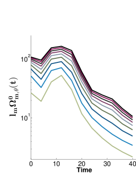
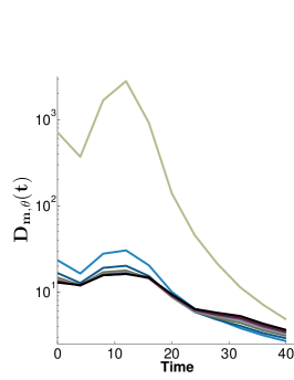
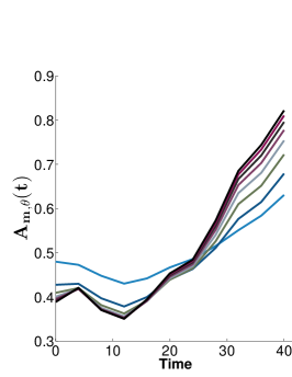
Figure 1: Time variation of: (a) $l_{m}\Omega_{m,\theta}(t)$, as defined in (18) ; (b) $D_{m,\theta}(t)$, as defined in (23) ; (c) $A_{m,\theta}(t)$ as defined in (28).

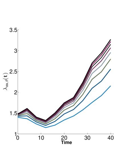
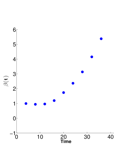
Figure 2: Time variation of: (a) $\lambda_{m,\theta}(t)$, as defined in (29), which fan out and grow with time ; (b) $\beta(t)$ as defined in (35).

Inserting (28) into the right hand side of (27) gives

$$\int_{\mathcal{V}}|\boldsymbol{\nabla}\theta|^{2}|\boldsymbol{\nabla}\mbox{\boldmath$u$}|\,dV \leq c_{1,m}D_{1,\omega}^{1/2}D_{1,\theta}^{(1+\lambda_{m,\theta})/2}$$ (30)

$$\leq \frac{1}{2}Pe_{0}D_{1,\omega}+c_{2,m}Pe_{0}^{-1}D_{1,\theta}^{1+\lambda_{m,\theta}}\,.$$

where the use of a Hölder inequality has split up the terms on the last line of the right hand side. The same idea is used on the last term in (26) with $|\boldsymbol{\nabla}\mbox{\boldmath$u$}|$ replaced by $|\Delta\theta|$ :

$$Pe_{0}^{-1}\int_{\mathcal{V}}|\boldsymbol{\nabla}\theta|^{2}|\Delta\theta|\,dV \leq \left(Pe_{0}^{-1}\|\Delta\theta\|_{2}^{2}\right)^{1/2}\left(2c_{3,m}Pe_{0}^{-1}D_{1,\theta}^{1+\lambda_{m,\theta}}\right)^{1/2}$$ (31)

$$\leq \frac{1}{2}Pe_{0}^{-1}\|\Delta\theta\|_{2}^{2}+c_{3,m}Pe_{0}^{-1}D_{1,\theta}^{1+\lambda_{m,\theta}}\,.$$

Altogether, (26) becomes

$$\frac{1}{2}\dot{D}_{1}\leq-\frac{1}{2}Pe_{0}^{-1}\|\Delta\theta\|_{2}^{2}+c_{4,m}Pe_{0}^{-1}D_{1,\theta}^{1+\lambda_{m,\theta}}+\frac{1}{2}Pe_{0}D_{1,\omega}\,.$$ (32)

A simple integration by parts shows that

$$\|\boldsymbol{\nabla}\theta\|_{2}^{2}\leq\|\Delta\theta\|_{2}\|\theta\|_{2}$$ (33)

and so we have

$$\frac{1}{2}\dot{D}_{1,\theta}\leq-\frac{1}{2}Pe_{0}^{-1}\frac{D_{1,\theta}^{2}}{\|\theta\|_{2}^{2}}+c_{4,m}Pe_{0}^{-1}D_{1,\theta}^{1+\lambda_{m,\theta}(t)}+\frac{1}{2}Pe_{0}D_{1,\omega}\,.$$ (34)

Because $\rho^{*}$ is bounded both below and above then so is $\|\theta\|_{2}^{2}$. Thus the competition on the right hand side of (34) in powers of $D_{1,\theta}$ lies between the negative $D_{1,\theta}^{2}$ term and either $Pe^{-1}D_{1,\theta}^{1+\lambda_{m,\theta}}$ or the $Pe_{0}D_{1,\omega}$ terms. To turn the differential inequality (34) into one in $D_{1,\theta}$ alone requires a relation between and $D_{1,\theta}$ and $D_{1,\omega}$, with the latter representing the fluid vorticity. Analytically, we have been unable to establish a relation between them but the JHT database provides us with the relation

$$D_{1,\omega}=D_{1,\theta}^{\beta(t)}\,,$$ (35)

where the growth in the exponent $\beta(t)$ is shown in figure 2b. Moreover, figure 3 shows that the $Pe_{0}D_{1,\theta}^{\beta(t)}$-term (plotted with blue squares) in (32) is dominant over the $Pe_{0}^{-1}D_{1,\theta}^{1+\lambda_{m,\theta}(t)}$-term (plotted with red circles), even when $\lambda_{m,\theta}(t)$ is chosen to be the maximum across $m$ at each particular time step. The plots of $1+\lambda_{m,\theta}$ and $\beta(t)$ both show that the values of these two quantities are both greater than $2$ and thus cannot be controlled by the $-D_{1,\theta}^{2}$ term in (34). $D_{1,\theta}$ is bounded only for extremely short times. Thus the possibility of the blow-up of $D_{1,\theta}$ in a finite time cannot be discounted.

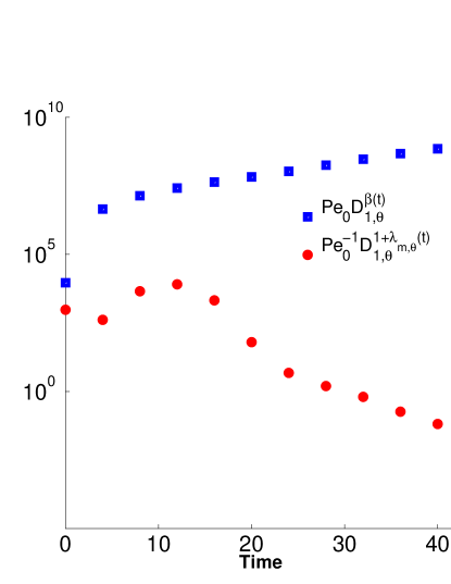
Figure 3: Time variation of $Pe_{0}D_{1,\theta}^{\beta(t)}$ (plotted with blue squares) and $Pe_{0}^{-1}D_{1,\theta}^{1+\lambda_{m,\theta}(t)}$-term (plotted with red circles) where $\lambda_{m,\theta}(t)$ is chosen to be the maximum value over $m$ at each time step with $Pe_{0}=12,500$.

Finally, figure 4 shows the equivalent set of plots of the time variation of $\ell_{m}\Omega_{m,\omega}(t)$, (as defined in (18) and (24)), $D_{m,\omega}(t)$ (as defined in (24)) and $A_{m,\omega}(t)$ defined as

$$A_{m,\omega}(t)=\ln D_{m,\omega}/\ln D_{1,\omega}.$$ (36)

In figure 5, we also show the time variation of the corresponding $\lambda_{m,\omega}(t)$, calculated using the analogous relationship

$$A_{m,\omega}(t)=\frac{\left[\lambda_{m,\omega}(t)(m-1)+1\right]}{(4m-3)}\,.$$ (37)

It is apparent that the turbulent fluid part of the problem, which drives and dominates the system, has corresponding $\lambda_{m,\omega}(t)$ that are flat in time and sit in the range $1<\lambda_{m,\omega}<2$. This is consistent with the behaviour found in three-dimensional Navier-Stokes flow described in Donzis et al (2013), Gibbon et al (2014) and Gibbon (2015). Note that this contrasts strongly with the behaviour of the $\theta$-variable where the $\lambda_{m,\theta}$ fan out and grow in time, as shown in figure 2.

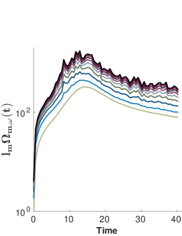
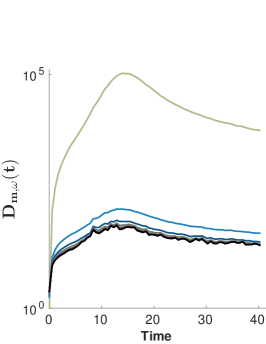
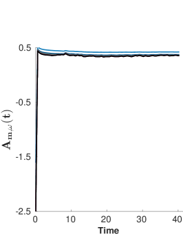
Figure 4: Time variation of: (a) $l_{m}\Omega_{m,\omega}(t)$ as defined in (18) ; (b) $D_{m,\omega}(t)$, as defined in (24) ; (c) $A_{m,\omega}(t)$, as defined in (37).

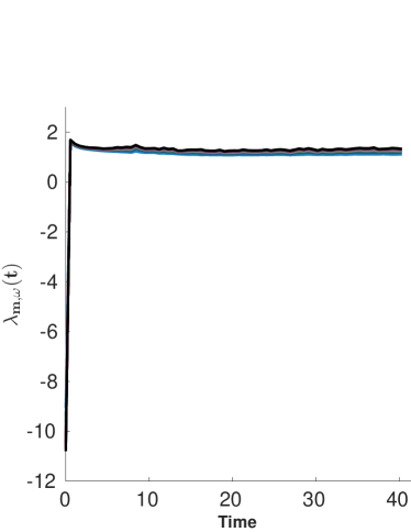
Figure 5: Time variation of $\lambda_{m,\omega}(t)$, calculated using the relation (37).

4 Conclusion

The numerical evidence in figure 2a suggests strong growth in $\lambda_{m,\theta}(t)$ which is consistent with strong growth in $\boldsymbol{\nabla}\rho^{*}$ even while $\rho^{*}$ is bounded. There are varying degrees of nonlinear depletion in the sense that $A_{m,\theta}<1$, and $A_{m,\omega}<1$ (as in figure 4c and 5). Depletion in $A_{m,\theta}$ reduces as the growth of $\lambda_{m,\theta}$ to the value $3.5$ in the final stages attests. Indeed, note that $\lambda_{m,\theta}=4$ would give a linear relation and be equivalent to a full estimate of the nonlinearity. Depletion in $D_{1,\omega}$ is quite severe, as shown in figures 4c and 5, which is consistent with the same effect observed in Navier-Stokes flows. Despite this, the cross-effect of the turbulent fluid flow driving the growth of $D_{1,\theta}$ through the exponent $\beta(t)$ swamps the term $D_{1,\theta}^{1+\lambda_{m,\theta}}$ in (34).

Following Livescu & Ristorcelli (2007), there is another way of looking at the growth in $\boldsymbol{\nabla}\rho^{*}$. Consider the equation for $\theta$ and introduce a new velocity field $\mathbi{v}=\mbox{\boldmath$u$}+Pe_{0}\boldsymbol{\nabla}\theta$. The Hopf-Cole-like transformation $\theta=\ln\rho$ in (14) then leads to an exact cancellation of the nonlinear terms in (15) to give

$$\left(\partial_{t}+\mathbi{v}\cdot\boldsymbol{\nabla}\right)\rho=Pe_{0}^{-1}\Delta\rho\,,\qquad\mbox{with}\qquad\boldsymbol{\nabla}.\mathbi{v}=0\,.$$ (38)

This is the linear advection diffusion equation driven by a divergence-free velocity field. Note that $\mbox{\boldmath$\omega$}=\mbox{curl}\,\mbox{\boldmath$u$}=\mbox{curl}\,\mathbi{v}$. The fact that $\mathbi{v}$ is actually an (explicit) function of $\boldsymbol{\nabla}\theta$ makes (38) less simple than it first appears.

Nevertheless, this equation provides a hint as to how we might look at the dynamics in a descriptive way. Consider a one-dimensional horizontal section through a rightward moving wave of $\rho^{*}$ at a snapshot in time : in the frame of the advecting velocity $u$ the relevant component of $\mathbi{v}$ is greater on the back face of any part of the wave (where $\boldsymbol{\nabla}\rho^{*}>0$) than on the front face (where $\boldsymbol{\nabla}\rho^{*}<0$). Thus in the advecting frame, (38) implies that not only is there the usual advection and diffusion but also a natural tendency for the back of a wave to catch up with the front, thus leading to steepening of $\boldsymbol{\nabla}\rho^{*}$. This is consistent with the evidence from (34) which leaves open the possibility that $D_{1,\theta}$ could blow up after a finite time or at least grow sufficiently strongly that the mixing is driven down to near molecular scales where the validity of the model fails. Interestingly, this then hints that buoyancy-driven turbulence may well be more intense in some sense than constant-density turbulence, which may explain the observed extremely efficient mixing possible in such flows.

Appendix A The equations for the composite density

Following Cook & Dimotakis (2001) and Livescu & Ristorcelli (2007) the composition density $\rho^{*}(\mathbi{x},\,t)$ of a mixture of two constant fluid densities $\rho^{*}_{1}$ and $\rho^{*}_{2}$ ($\rho^{*}_{2}>\rho^{*}_{1}$) is expressed by (2) where $Y(\mathbi{x},\,t)=Y_{2}$ is the mass fraction of the heavier fluid. It is important to stress that the two fluids are assumed to be incompressible, yet we do not make the Boussinesq approximation and so the difference between the two densities is allowed to take arbitrary values. Under the transport of a (dimensionless) velocity field $\mbox{\boldmath$u$}(\mathbi{x},\,t)$, $\rho^{*}$ obeys the equation of conservation of mass

$$\partial_{t}\rho^{*}+\boldsymbol{\nabla}\cdot(\rho^{*}\mbox{\boldmath$u$})=0\,,$$ (39)

and the species transport equation

$$\partial_{t}(\rho^{*}Y)+\boldsymbol{\nabla}\cdot\left(\rho^{*}Y\mbox{\boldmath$u$}+\mbox{\boldmath$j$}_{F}\right)=0\,,$$ (40)

where the divergence of the flux $\mbox{\boldmath$j$}_{F}$ represents Fickian diffusion, i.e.

$$\mbox{\boldmath$j$}_{F}=-Pe_{0}^{-1}\rho^{*}\boldsymbol{\nabla}Y\,.$$ (41)

where the Péclet number has been defined in table 1. Given that the solution of (2) shows that $\rho^{*}Y$ is linear in $\rho^{*}$ such that

$$\rho^{*}Y=a\rho^{*}+b\,,\qquad a=\frac{\rho^{*}_{2}}{\rho^{*}_{2}-\rho^{*}_{1}}\,,\qquad b=-\frac{\rho^{*}_{1}\rho^{*}_{2}}{\rho^{*}_{2}-\rho^{*}_{1}}\,,$$ (42)

equation (40) simplifies to

$$b\,\boldsymbol{\nabla}\cdot\mbox{\boldmath$u$}=Pe_{0}^{-1}\boldsymbol{\nabla}\cdot(\rho^{*}\boldsymbol{\nabla}Y)\,.$$ (43)

Noting from (42) that $\rho^{*}\boldsymbol{\nabla}Y=-b\boldsymbol{\nabla}(\ln\rho^{*})$ the coefficient $b$ cancels to make (43) and (39) into :

$$\boldsymbol{\nabla}\cdot\mbox{\boldmath$u$}=-Pe_{0}^{-1}\Delta(\ln\rho^{*})\,.$$ (44)

$$\left(\partial_{t}+\mbox{\boldmath$u$}\cdot\boldsymbol{\nabla}\right)\rho^{*}=Pe_{0}^{-1}\rho^{*}\Delta(\ln\rho^{*})\,.$$ (45)

An interesting observation is that using a normalization density $\rho^{*}_{0}$ and with the definition

$$\theta(\mathbi{x},\,t)=\ln\rho\qquad\qquad\rho=\frac{\rho^{*}}{\rho^{*}_{0}}\,.$$ (46)

(45) becomes a deceptively innocent-looking diffusion-like equation

$$\left(\partial_{t}+\mbox{\boldmath$u$}\cdot\boldsymbol{\nabla}\right)\theta=Pe_{0}^{-1}\Delta\theta\,,$$ (47)

with an equation for $\boldsymbol{\nabla}\cdot\mbox{\boldmath$u$}$ that depends on two derivatives of $\theta$

$$\boldsymbol{\nabla}\cdot\mbox{\boldmath$u$}=-Pe_{0}^{-1}\Delta\theta\,.$$ (48)

Appendix B Proof of the boundedness of $\|\rho^{*}\|_{L^{\infty}(\mathcal{V})}$

To prove the boundedness of $\|\rho^{*}\|_{L^{\infty}(\mathcal{V})}$ under a sufficiently regular advecting field $u$ we write

$$\frac{1}{2m}\frac{d~{}}{dt}\int_{\mathcal{V}}|\rho^{*}|^{2m}dV=-\int_{\mathcal{V}}\rho^{*(2m-1)}\,\boldsymbol{\nabla}\cdot(\rho^{*}\mbox{\boldmath$u$})\,dV\,,$$ (49)

and

$$\rho^{*(2m-1)}\,\boldsymbol{\nabla}\cdot(\rho^{*}\mbox{\boldmath$u$})=\left(1-\frac{1}{2m}\right)\rho^{*2m}\,\boldsymbol{\nabla}\cdot\mbox{\boldmath$u$}+\frac{1}{2m}\boldsymbol{\nabla}\cdot(\rho^{*2m}\mbox{\boldmath$u$})\,.$$ (50)

(49) then becomes

$$\frac{1}{2m}\frac{d~{}}{dt}\int_{\mathcal{V}}|\rho^{*}|^{2m}dV=-\left(1-\frac{1}{2m}\right)\int_{\mathcal{V}}\rho^{*2m}\,\boldsymbol{\nabla}\cdot\mbox{\boldmath$u$}\,dV$$ (51)

where the volume integral of the second term in (50) is zero through the Divergence Theorem. Using (12), (51), becomes

$$\frac{1}{2m}\frac{d~{}}{dt}\int_{\mathcal{V}}|\rho^{*}|^{2m}dV = Pe_{0}^{-1}\left(1-\frac{1}{2m}\right)\int_{\mathcal{V}}\rho^{*2m}\,\Delta(\ln\rho^{*})\,dV$$ (52)

$$= -Pe_{0}^{-1}(2m-1)\int_{\mathcal{V}}\rho^{*2(m-1)}|\boldsymbol{\nabla}\rho^{*}|^{2}\,dV$$

$$= -Pe_{0}^{-1}\frac{(2m-1)}{m^{2}}\int_{\mathcal{V}}|\boldsymbol{\nabla}\rho^{*m}|^{2}\,dV$$

so Poincaré’s inequality shows each norm $\|\rho^{*}\|_{L^{2m}(\mathcal{V})}$ decays exponentially from its initial conditions. In the limit $m\to\infty$, $\|\rho^{*}\|_{L^{\infty}(\mathcal{V})}$ is bounded by its initial conditions. $\blacksquare$

References

- Andrews & Dalziel (2010) Andrews, M. J. & Dalziel, S. B. 2010 Small Atwood number Rayleigh-Taylor experiments. Phil. Trans. R. Soc. Ser. A 368 (1916), 1663–79.
- Cabot & Cook (2006) Cabot, W. H. & Cook, A. W. 2006 Reynolds number effects on Rayleigh-Taylor instability with possible implications for type Ia supernovae. Nat. Phys. 2 (8), 562–568.
- Cook & Dimotakis (2001) Cook, A. W. & Dimotakis, P. E. 2001 Transition stages of Rayleigh-Taylor instability between miscible fluids. J. Fluid Mech. 443, 69–99.
- Davies-Wykes & Dalziel (2014) Davies-Wykes, M. S. & Dalziel, S. B. 2014 Efficient mixing in stratified flows: experimental study of a Rayleigh-Taylor unstable interface within an otherwise stable stratification.
- Dimonte et al. (2004) Dimonte, G., Youngs, D. L., Dimits, A., Weber, S., Marinak, M., Wunsch, S., Garasi, C., Robinson, A., Andrews, M. J., Ramaprabhu, P., Calder, A. C., Fryxell, B., Biello, J., Dursi, L., MacNeice, P., Olson, K., Ricker, P., Rosner, R., Timmes, F., Tufo, H., Young, Y.-N. & Zingale, M. 2004 A comparative study of the turbulent Rayleigh-Taylor instability using high-resolution three-dimensional numerical simulations: The Alpha-Group collaboration. Phys. Fluids 16, 1668–1693.
- Dimotakis (2005) Dimotakis, P. E. 2005 Turbulent mixing. Annu. Rev. Fluid Mech. 37, 329–356.
- Donzis et al. (2013) Donzis, D.A., Gibbon, J.D., Kerr, R.M., Gupta, A., Pandit, R. & Vincenzi, D. 2013 Vorticity moments in four numerical simulations of the Navier-Stokes equations. J. Fluid Mech. 732, 316–331.
- Gibbon et al. (2014) Gibbon, J.D., Donzis, D. A., Kerr, R.M., Gupta, A., Pandit, R. & Vincenzi, D. 2014 Regimes of nonlinear depletion and regularity in the navier-stokes equations. Nonlinearity 27, 1–19.
- Gibbon (2015) Gibbon, J. D. 2015 High-low frequency slaving and regularity issues in the 3d Navier-Stokes equations. IMA Journal of Applied Mathematics pp. 1–13.
- Glimm et al. (2001) Glimm, J., Grove, J. W., Li, X. L., Oh, W. & Sharp, D. H. 2001 A critical analysis of Rayleigh-Taylor growth rates. J. Comp. Phys. 169 (2), 652–677.
- Hyunsun et al. (2008) Hyunsun, L., Hyeonseong, J., Yan, Y. & Glimm, J. 2008 On validation of turbulent mixing simulations for Rayleigh-Taylor instability. Phys. Fluids 20, 012102–012102–8.
- Lawrie & Dalziel (2011) Lawrie, A. G. W. & Dalziel, S. B. 2011 Rayleigh-Taylor mixing in an otherwise stable stratification. J. Fluid Mech. 688, 507–527.
- Lee et al. (2008) Lee, H., Jin, H., Yu, Y. & Glimm, J. 2008 On validation of turbulent mixing simulations for Rayleigh-Taylor instability. Phys. Fluids 20, 1–8.
- Livescu (2013) Livescu, D. 2013 Numerical simulations of two-fluid mixing at large density ratios and applications to the Rayleigh-Taylor instability. Phil. Trans. R. Soc. A. 371, 20120185.
- Livescu et al. (2014) Livescu, D., Canada, C., Kanov, K., Burns, R. & Pulido, J. 2014 Homogeneous buoyancy driven turbulence data set. LA-UR-14-20669 .
- Livescu et al. (2009) Livescu, D., Mohd-Yusof, J., Petersen, M.R. & Grove, J.W. 2009 A computer code for direct numerical simulation of turbulent flows. Tech. Rep. LA-CC-09-100. Los Alamos National Laboratory.
- Livescu & Ristorcelli (2007) Livescu, D. & Ristorcelli, J. R. 2007 Buoyancy-driven variable-density turbulence. J. Fluid Mech. 591, 4–71.
- Livescu & Ristorcelli (2008) Livescu, D. & Ristorcelli, J. R. 2008 Variable-density mixing in buoyancy-driven turbulence. J. Fluid Mech. 605, 145–180.
- Petrasso (1994) Petrasso, R. D. 1994 Rayleigh’s challenge endures. Nat. Phys. 367 (6460), 217–218.
- Rayleigh (1900) Rayleigh, Lord 1900 Investigation of the character of the equilibrium of an incompressible heavy fluid of variable density. Scientific Papers 2, 598.
- Sharp (1984) Sharp, D. H. 1984 An overview of Rayleigh-Taylor Instability. Physica D 12D, 3–18.
- Tailleux (2013) Tailleux, R. 2013 Available potential energy and exergy in stratified fluids. Annu. Rev. Fluid Mech. 45, 35–58.
- Taylor (1950) Taylor, G. I. 1950 The instability of liquid surfaces when accelerated in a direction perpendicular to their planes. I. Proc. R. Soc. A 201 (1065), 192–196.
- Youngs (1984) Youngs, David L. 1984 Numerical simulation of turbulent mixing by Rayleigh-Taylor instability. Physica D: Nonlinear Phenomena 12 (1-3), 32–44.
- Youngs (1989) Youngs, David L. 1989 Modelling turbulent mixing by Rayleigh-Taylor instability. Physica D: Nonlinear Phenomena 37, 270–287.