CRIME MODELING WITH TRUNCATED LÉVY FLIGHTS FOR RESIDENTIAL BURGLARY MODELS

Abstract

Statistical agent-based models for crime have shown that repeat victimization can lead to predictable crime hotspots (see e.g. Short et al., Math. Models Methods Appl., $2008$), then a recent study in one space dimension (Chaturapruek et al., SIAM J. Appl. Math, $2013$) shows that the hotspot dynamics changes when movement patterns of the criminals involve long-tailed Lévy distributions for the jump length as opposed to classical random walks. In reality criminals move in confined areas with a maximum jump length. In this paper we develop a mean-field continuum model with truncated Lévy flights for residential burglary in one space dimension. The continuum model yields local Laplace diffusion, rather than fractional diffusion. We present an asymptotic theory to derive the continuum equations and show excellent agreement between the continuum model and the agent-based simulations. This suggests that local diffusion models are universal for continuum limits of this problem, the important quantity being the diffusion coefficient. Law enforcement agents are also incorporated into the model, and the relative effectiveness of their deployment strategies are compared quantitatively.

(xxxxxxxxxx)

AMS Subject Classification: 35R60, 35Q84, 60G50.

1 Introduction

Residential crime is one of the toughest issues in modern society. A quantitative, informative and applicable model of crime is needed to assist law enforcement. Crimes of opportunity often have consistent statistical properties, and it is possible to model them using quantitative tools.[38] In the past ten years applied mathematicians have been working in the burgeoning area of crime modeling and prediction (see e.g. Refs. bellomo-Berestycki2013, Gorr2014-Goudon, koloko, Tijana, lloyd, Ajmone, mccalla2013, mohler2011-uclaModel, wardurban-Zipkin), since the seminal work Ref. uclaModel on the mathematics of agent-based models for residential burglary.

Roughly speaking, there are two classes of burglary models. Class I is statistical in nature aiming to predict the patterns of observed events. Among them, self-exciting point process models in Ref. mohler2011 have led to the development of software products for field use [29]. Class II is agent-based and describes the actions of individuals that lead to aggregate pattern formation. It is this class of models that we address here. Agent-based models could be used for prediction if all model parameters were known. Parameters for environmental variables can be well estimated from field data, however movement patterns of individual burglars are difficult to track. Therefore, it is imperative to identify the simplest class of universal models for criminal movement.

Ref. uclaModel used a biased random walk, that is, short hops, for criminal agents. It is well-known that people foraging in an environment are more likely to move according to a Lévy flight than a random walk[9, 3, 13]. A later paper[6] analyzed such processes for this model and showed that such processes lead to fractional diffusion rather than classical Brownian motion in the continuum. Here we refocus the analysis to truncated Lévy flights since they are the most realistic. The truncation size represents the maximum mobility of an agent. We show that an analogue mean-field continuum model exists with local diffusion replacing fractional diffusion. Specifically, for a range of length scales truncated Lévy flights behave similarly to a Brownian process with a modified diffusion coefficient.

As for the coupling of the dynamics of criminals and of the environment variables, following Ref. uclaModel, we incorporate the repeat and near-repeat victimization and the broken windows effect. These are concepts in criminology and sociology that have been empirically observed[4, 8, 12]. Specifically, residential burglars prefer to return to a previously burglarized house and its neighbors[7, 14, 15, 16, 37]. These are known as repeat and near-repeat events. Also according to the “broken windows” theory, it is very likely that the visible signs of the past crimes in a neighborhood may create an environment that encourages further illegal activities [41].

In addition following Ref. law_enforcement, we introduce the effects of law enforcement agents into the model. In Ref. law_enforcement, all the agents are assumed to take random walks, while here law enforcement agents follow truncated Lévy flights whose maximum jump length can be different from that of the criminals. The relative effectiveness of several policing strategies is compared quantitatively.

This is the first time that truncated Lévy flights have been applied in crime modeling. Previously they have only been applied in other areas such as finance [23, 25, 27] and networks.[5]

The article is organized as follows. In Sec. 2, we introduce the discrete model and compare it for different values of the jump length. In Sec. 3, we derive the mean-field continuum model and compare it with the discrete model through computer simulations. Next in Sec. 4, we incorporate law enforcement agents into the system, derive the continuum equations, and then compare the relative effectiveness of the deployment strategies both quantitatively and qualitatively.

2 Discrete Model

2.1 Overview

As in Ref. levycrime, the system is defined on a one-dimensional grid which represents the stationary burglary sites. We assume constant grid lattice spacing $l$ and periodic boundary conditions. Our model consists of two components — the stationary burglary sites and a collection of burglar agents jumping from site to site. The system evolves only at discrete time steps $t=n\delta t,n\in\mathbb{N}$, $\delta t>0$. Attached to each grid $k\in\mathbb{Z}$ is a vector $({n}_{k}(t),A_{k}(t))$, representing the number of criminals and the “attractiveness” at site $k$ at time $t$. The attractiveness refers to the burglar’s beliefs about the vulnerability and value of the target site and it is assumed to consist of a static background term and a dynamic term:

$${A}_{k}(t)=A_{k}^{0}+{B}_{k}(t).$$ (1)

The dynamic term $B_{k}(t)$ represents the component associated with repeat victimization and broken windows effect, whose behavior will be discussed shortly. Our model unfolds starting with some initial distribution of criminal agents and attractiveness field over the lattice grid. At each time step, the system gets updated as follows:

Step 1. Every criminal decides if he will commit a burglary at his current site with probability

$$p_{k}(t)=1-e^{-A_{k}(t)\delta t}.$$ (2)

This means that the Poisson instantaneous burglary rate is roughly $A_{k}(t)$, and $A_{k}(t)\delta t$ is the expected number of burglary events in the time interval of length $\delta t$ from a single burglar at site $k$.

Step 2. If a criminal agent chooses to commit a burglary then he will be immediately removed from the system. Otherwise he will move to another site according to a truncated Lévy distribution biased towards areas with a high attractiveness. More specifically, the probability of an agent jumping from site $k$ to $i$ is

$$q_{k\rightarrow i}(t)=\dfrac{w_{k\rightarrow i}(t)}{\sum\limits_{\begin{subarray}{c}j\in\mathbb{Z}\\ j\neq k\end{subarray}}{w_{k\rightarrow j}(t)}},\quad\quad k\neq i,$$ (3)

where the corresponding relative weight $w_{k\rightarrow i}(t)$ is defined as

$$w_{k\rightarrow i}(t)=\begin{cases}\dfrac{A_{i}(t)}{l^{\mu}|i-k|^{\mu}},&1\leq|i-k|\leq L,\\ 0,&\text{otherwise}.\end{cases}$$ (4)

Here $\mu\in(1,3)$ is the exponent of the underlying power law of the Lévy distribution, and $L\in\mathbb{N}$ is the truncation size. These parameters represent the mobilities of the criminal agents. Different types of agents often assume different mobilities. For example, the parameter $\mu$ for professional criminals is typically lower than that of amateur criminals.[19, 39] We call the movement pattern defined by (3) and (4) a truncated Lévy flight (TLF). When $L=\infty$, we call it a Lévy flight. When $L=1$, then (3) and (4) imply

$$q_{k\rightarrow i}(t)=\dfrac{A_{i}(t)}{A_{k-1}(t)+A_{k+1}(t)},\quad\quad i=k-1\mbox{ or }i=k+1,$$

and we call this a biased random walk (BRW). If the random walk is unbiased, that is, if $q_{k\rightarrow k-1}(t)=q_{k\rightarrow k-1}=1/2$, then we call it an unbiased random walk (URW).

Step 3. The attractiveness field gets updated according to the repeat victimization and the broken windows effect.[4, 8, 12] The repeat victimization is introduced by letting the dynamic attractiveness depend upon previous burglary events at the local site. Whenever there is a burglary event, the local attractiveness will get increased by an absolute constant $\theta$. However it is reasonable to suppose that this higher probability of burglary at a site has a finite lifetime. This increase and decay can be modeled according to the following update rule

$${B}_{k}(t+\delta t)={B}_{k}(t)(1-\omega\delta t)+\theta{E}_{k}(t),$$

where $\omega$ is an absolute constant representing the decay rate, and $E_{k}(t)$ denotes the number of burglary events occurred during the time interval $(t,t+\delta t]$ at site $k$. To further incorporate the broken windows effect, we allow the dynamic attractiveness field to spread spatially from each site to its nearest neighbours. This can be accomplished by modifying the above equation as

$${B}_{k}(t+\delta t)=\left[(1-\eta){B}_{k}(t)+\dfrac{\eta}{2}({B}_{k-1}(t)+{B}_{k+1}(t))\right](1-\omega\delta t)+\theta{E}_{k}(t),$$

where $\eta\in(0,1)$ is an absolute constant representing the strength of the near-repeat victimization effect. Since on average the attractiveness can be roughly expressed by replacing $E_{k}(t)$ with $\delta tA_{k}(t){n}_{k}(t)$ according to (2), we finally set the evolution of the dynamic attractiveness term as

$${B}_{k}(t+\delta t)=\left[(1-\eta){B}_{k}(t)+\dfrac{\eta}{2}({B}_{k-1}(t)+{B}_{k+1}(t))\right](1-\omega\delta t)+\theta\delta tA_{k}(t){n}_{k}(t).$$ (5)

Step 4. At each site a new agent is replaced with rate $\gamma$.

Figure 1 presents a visual summary of these four steps in the form of a flow chat.

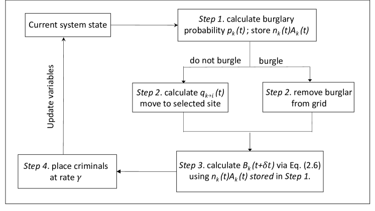
Fig. 1: Flowchart summarizing the discrete model.

To conclude, the discrete mean field equation of $(A_{k}(t),n_{k}(t))$ consists of (5) and the following equation

$${n}_{k}(t+\delta t)=\sum_{\begin{subarray}{c}i\in\mathbb{Z}\\ 1\leq|i-k|\leq L\end{subarray}}{[1-A_{i}(t)\delta t]{n}_{i}(t)q_{i\rightarrow k}(t)}+\gamma\delta t.$$ (6)

When $L=1$ and $L=\infty$, the assumptions above yield respectively the random-walk model (RWM) in Ref. uclaModel, and the Lévy-flight model (LFM) in Ref. levycrime. Hence our first task is to see how varying $L$ will affect the behavior of the truncated-Lévy-flight model (TLFM).

2.2 Computer simulations

We simulate the truncated-Lévy-flight model for several different values of jump length $L$. An example output can be seen in Fig. 2 below. The domain is $[0,1]$ and ${l}=1/60$. The computations assume periodic boundary conditions. Here the initial conditions (at $t=0$) are taken to be $B_{k}\equiv 0$ and ${{n}}_{k}\equiv 1$. The parameters are $A^{0}=1-0.4\cos(4\pi x)$, $\mu=2.5$, $l=1/60$, $\delta t=0.01$, ${\eta}=0.1$, $\gamma=6$, $\omega=1$, and $\theta=1$.

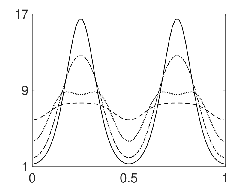
(a) $t=8$

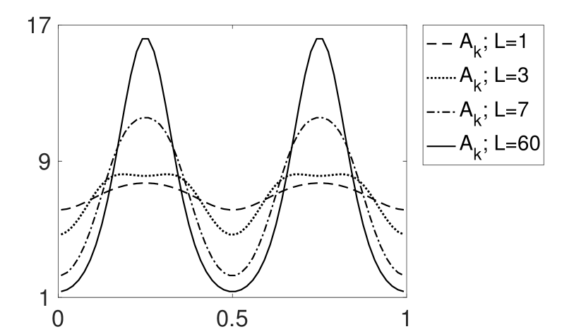
(b) $t=20$

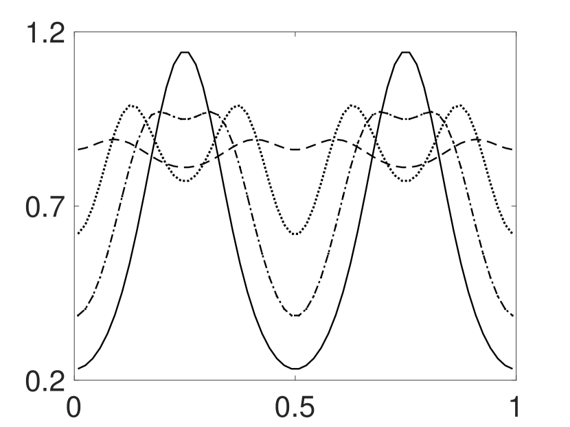
(c) $t=8$

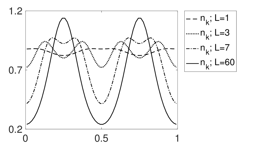
(d) $t=20$

Fig. 2: Results of the model (1)-(5) for different values of $L$, using the parameters described in the text. The plots of the attractiveness field are shown in (a), (b), and the plots of the criminal number distribution are shown in (c), (d). For $L=1$, $3$, $7$, and $60$, they are shown respectively with dashed lines, dotted lines, dash-dotted lines, and solid lines.

We observe that the behavior of the model varies considerably with different choices of $L$. This was already noted in the prior work Ref. levycrime. This suggests that more careful analysis should be carried out to connect the two ideas. Here we show that truncation is precisely the correct parameter for this research direction.

3 Continuum Model

3.1 Derivation

In this section, we derive an asymptotic theory when $\delta t$ and $l$ become small under some suitable spatial-temporal scaling for generic $L\in\mathbb{N}$.

We first derive the dynamics of the continuum version of the attractiveness field. Following Ref. uclaModel, we observe that the Brownian scaling is a suitable spatial-temporal scaling for (5). That is, as ${l}$ and $\delta t$ become smaller, the quantity ${l}^{2}/\delta t$ remains constant. Using the same calculations as in Ref. uclaModel, from (5) and (1) we infer

$$\dfrac{\partial A}{\partial t}=\dfrac{l^{2}\eta}{2\delta t}A_{xx}-\omega(A-A^{0})+\theta{n}A.$$ (7)

The derivation of the dynamics of the continuum version of ${n}_{k}$, however, is more complicated. From (6) we infer

$$\dfrac{{n}_{k}(t+\delta t)-{n}_{k}(t)}{\delta t}=\dfrac{1}{\delta t}\left[\sum_{\begin{subarray}{c}i\in\mathbb{Z}\\ 1\leq|i-k|\leq L\end{subarray}}{n}_{i}(1-A_{i}\delta t)q_{i\rightarrow k}-{n}_{k}\right]+\gamma.$$ (8)

We define

$$z_{\mu,L} :=2\sum_{k=1}^{L}\dfrac{1}{k^{\mu}},$$ (9)

$$\mathcal{L}(f_{i}) :=\sum_{\begin{subarray}{c}j\in\mathbb{Z}\\ 1\leq|i-j|\leq L\end{subarray}}\dfrac{f_{j}-f_{i}}{(|j-i|l)^{\mu}}.$$ (10)

It follows from (4) that

$$\sum_{\begin{subarray}{c}i\in\mathbb{Z}\\ 1\leq|i-k|\leq L\end{subarray}}{w_{i\rightarrow k}}=l^{-\mu}z_{\mu,L}A_{i}+\mathcal{L}(A_{i}).$$ (11)

With (11) and (3), we obtain

$$q_{i\rightarrow k} =\dfrac{w_{i\rightarrow k}}{l^{-\mu}z_{\mu,L}A_{i}\left(\dfrac{\mathcal{L}(A_{i})}{l^{-\mu}z_{\mu,L}A_{i}}+1\right)}$$

$$\sim w_{i\rightarrow k}\left[\dfrac{1}{l^{-\mu}z_{\mu,L}A_{i}}-\dfrac{\mathcal{L}(A_{i})}{(l^{-\mu}z_{\mu,L}A_{i})^{2}}\right]$$

$$=\dfrac{A_{k}}{|i-k|^{\mu}}\left(\dfrac{1}{z_{\mu,L}A_{i}}-\dfrac{\mathcal{L}(A_{i})l^{\mu}}{A_{i}^{2}z_{\mu,L}^{2}}\right),\hskip 14.22636pt1\leq|i-k|\leq L.$$ (12)

Here we have used the fact that ${1}/({1+x})$ approximates $1-x$ as long as $x^{2}\sim o(1)$. Applying (12) to the right-hand-side of (8), we obtain

$$\!\!\!\!\!\!\dfrac{{n}_{k}(t+\delta t)-{n}_{k}(t)}{\delta t} =\dfrac{1}{\delta t}\!\!\!\!\sum_{\begin{subarray}{c}i\in\mathbb{Z}\\ 1\leq|i-k|\leq L\end{subarray}}\!\!\!\!{{n}_{i}(1-A_{i}\delta t)\dfrac{A_{k}}{|i-k|^{\mu}}\left(\dfrac{1}{z_{\mu,L}A_{i}}-\dfrac{\mathcal{L}(A_{i})l^{\mu}}{A_{i}^{2}z_{\mu,L}^{2}}\right)}-\dfrac{{n}_{k}}{\delta t}+\gamma$$

$$=\dfrac{A_{k}}{\delta t}\left[\sum_{\begin{subarray}{c}i\in\mathbb{Z}\\ 1\leq|i-k|\leq L\end{subarray}}(1-A_{i}\delta t){\dfrac{{n}_{i}}{A_{i}}\dfrac{1}{z_{\mu,L}|i-k|^{\mu}}}-\dfrac{{n}_{k}}{A_{k}}\right]$$

$$\hskip 14.22636pt-\dfrac{A_{k}}{\delta t}\sum_{\begin{subarray}{c}i\in\mathbb{Z}\\ 1\leq|i-k|\leq L\end{subarray}}\left[(1-A_{i}\delta t)\dfrac{{n}_{i}}{|i-k|^{\mu}}\dfrac{\mathcal{L}(A_{i})l^{\mu}}{A_{i}^{2}z_{\mu,L}^{2}}\right]+\gamma.$$ (13)

In order to simplify (13), from (10) we infer

$$\sum_{{\begin{subarray}{c}i\in\mathbb{Z}\\ 1\leq|i-k|\leq L\end{subarray}}}\!\!\!\!\!\dfrac{{n}_{i}}{|i-k|^{\mu}}=\sum_{{\begin{subarray}{c}i\in\mathbb{Z}\\ 1\leq|i-k|\leq L\end{subarray}}}\!\!\!\!\!\!\dfrac{{n}_{i}-{n}_{k}}{|i-k|^{\mu}}+\sum_{{\begin{subarray}{c}i\in\mathbb{Z}\\ 1\leq|i-k|\leq L\end{subarray}}}\!\!\!\!\!\!\dfrac{{n}_{k}}{|i-k|^{\mu}}=l^{\mu}\mathcal{L}({n}_{k})+z_{\mu,L}{n}_{k}\sim z_{\mu,L}{n}_{k},$$

where the $O(l^{\mu})$ terms have been ignored in the final step. This together with (13) implies that

$$\dfrac{{n}_{k}(t+\delta t)-{n}_{k}(t)}{\delta t} =\dfrac{A_{k}}{\delta t}\!\!\!\!\sum_{\begin{subarray}{c}i\in\mathbb{Z}\\ 1\leq|i-k|\leq L\end{subarray}}\!\!\!\!\!\left[\dfrac{{n}_{i}}{A_{i}}\dfrac{1}{z_{\mu,L}|i-k|^{\mu}}-\delta t\dfrac{{n}_{i}}{|i-k|^{\mu}z_{\mu,L}}-\dfrac{{n}_{k}}{A_{k}}\dfrac{1}{z_{\mu,L}|i-k|^{\mu}}\right]$$

$$\hskip 14.22636pt-\dfrac{A_{k}}{\delta t}\!\!\!\!\sum_{\begin{subarray}{c}i\in\mathbb{Z}\\ 1\leq|i-k|\leq L\end{subarray}}\left[\dfrac{{n}_{i}}{|i-k|^{\mu}}\!\!\!\!\!\ \dfrac{\mathcal{L}(A_{i})l^{\mu}}{A_{i}^{2}z_{\mu,L}^{2}}-\dfrac{{n}_{i}\mathcal{L}A_{i}}{A_{i}zz_{\mu,L}^{2}|i-k|^{\mu}}l^{\mu}\delta t\right]+\gamma$$

$$\sim\dfrac{A_{k}}{\delta t}\!\!\!\!\!\!\!\!\sum_{\begin{subarray}{c}i\in\mathbb{Z}\\ 1\leq|i-k|\leq L\end{subarray}}\!\!\left[{\dfrac{\dfrac{{n}_{i}}{A_{i}}\!-\!\dfrac{{n}_{k}}{A_{k}}}{|i-k|^{\mu}z_{\mu,L}}}\!-\!\dfrac{{n}_{i}}{|i-k|^{\mu}}\dfrac{\mathcal{L}(A_{i})l^{\mu}}{A_{i}^{2}z_{\mu,L}^{2}}\!-\!\delta t\dfrac{{n}_{i}}{|i-k|^{\mu}z_{\mu,L}}\right]\!\!+\!\!\gamma$$

$$\sim\dfrac{l^{\mu}}{z_{\mu,L}\delta t}\left[A_{k}\mathcal{L}\left(\dfrac{{n}_{k}}{A_{k}}\right)-\dfrac{{n}_{k}\mathcal{L}(A_{k})}{A_{k}}\right]-A_{k}{n}_{k}+\gamma.$$ (14)

Here at the second step, all the $O(l^{\mu}\delta t)$ terms have been ignored in the summation. We now simplify

$$\mathcal{L}(A_{k})=\sum_{\begin{subarray}{c}j\in\mathbb{Z}\\ 1\leq|j-k|\leq L\end{subarray}}{\dfrac{A_{j}-A_{k}}{(|j-k|l)^{\mu}}}.$$ (15)

Let $x=kl$ and then $A_{k}=A(x)$. When $l$ is small, we can apply the Taylor expansion to the integrand near $x$ and obtain

$$\mathcal{L}(A_{k}) =\!\!\!\!\!\sum_{\begin{subarray}{c}j\in\mathbb{Z}\\ 1\leq|j-k|\leq L\end{subarray}}{{\!\!\!\!\!(|j-k|l)^{-\mu}}\left[{A_{x}(kl)(j-k)l+A_{xx}(kl)\dfrac{((j-k)l)^{2}}{2}+\!O((|j-k|l)^{3})}\right]}$$

$$\sim\left[\sum_{\begin{subarray}{c}j\in\mathbb{Z}\\ 1\leq|j-k|\leq L\end{subarray}}{\dfrac{A_{x}(kl)(j-k)l}{(|j-k|l)^{\mu}}}+\sum_{\begin{subarray}{c}j\in\mathbb{Z}\\ 1\leq|j-k|\leq L\end{subarray}}{\dfrac{A_{xx}(kl)((j-k)l)^{2}}{2(|j-k|l)^{\mu}}}\right]$$

$$=\frac{1}{2}\sum_{\begin{subarray}{c}j\in\mathbb{Z}\\ 1\leq|j-k|\leq L\end{subarray}}{{(|j-k|l)^{2-\mu}}A_{xx}(kl)}$$

$$={l^{2-\mu}}\sum_{j=1}^{L}j^{2-\mu}A_{xx}(kl).$$ (16)

Here at the second step, the $O((|j-k|l)^{3-\mu})$ terms and lower order terms are all ignored as $\mu<3$. We then obtain

$$\mathcal{L}(A_{k})={l^{2-\mu}}z^{\ast}_{\mu,L}A_{xx}(kl),$$ (17)

where

$$z^{\ast}_{\mu,L}:=\sum_{j=1}^{L}j^{2-\mu}.$$ (18)

From (17) and (14) we infer

$$\dfrac{\partial{n}}{\partial t}=\mathcal{D}\vec{\nabla}\cdot\left[\vec{\nabla}{n}-\dfrac{2{n}}{A}\vec{\nabla}A\right]-A{n}+\gamma,$$ (19)

where

$$\mathcal{D}=\dfrac{l^{2}}{\delta t}\frac{z^{\ast}_{\mu,L}}{z_{\mu,L}}.$$ (20)

Here $\mathcal{D}$ is the diffusion coefficient which depends on $\mu$ and $L$. Particularly when $L=1$, then $\mathcal{D}=l^{2}/2\delta t$.

To validate the continuum model we next perform direct numerical simulations and compare it with the discrete model.

Remark 3.1.

When $L=1$ and $L=\infty$, we recall that the mean field continuum equations of the random-walk model (RWM) and the Lévy-flight model (LFM) have been derived in Refs. uclaModel and levycrime:

$$\mbox{Continuum RWM }\begin{cases}&\!\!\!\!\!\dfrac{\partial A}{\partial t}=\dfrac{l^{2}\eta}{2\delta t}A_{xx}-\omega(A-A^{0})+\theta A{{n}},\\ \\ &\!\!\!\!\!\dfrac{\partial{n}}{\partial t}=\dfrac{l^{2}}{2\delta t}\vec{\nabla}\cdot\left[\vec{\nabla}{n}-\dfrac{2{n}}{A}\vec{\nabla}A\right]-{A}{{{n}}}+\gamma,\end{cases}$$ (21)

$$\mbox{Continuum LFM }\begin{cases}&\!\!\!\!\!\dfrac{\partial A}{\partial t}=\dfrac{l^{2}\eta}{2\delta t}A_{xx}-\omega(A-A^{0})+\theta A{{n}},\\ \\ &\!\!\!\!\!\dfrac{\partial{n}}{\partial t}=\dfrac{l^{2s}}{\delta t}\dfrac{\sqrt{\pi}2^{-2s}|\Gamma(-s)|}{z\Gamma(s+\dfrac{1}{2})}\left[{A}\Delta^{s}(\dfrac{{{{n}}}}{{A}})-\dfrac{{{{n}}}}{{A}}\Delta^{s}{A}\right]-{A}{{{n}}}+\gamma.\end{cases}$$ (22)

Here $s=\left({\mu-1}\right)/{2}$, $z=2\sum_{k=1}^{\infty}k^{-\mu}$, and $\Gamma(\cdot)$ denotes the gamma function. We also note that when $L=1$, (19) coincides with (21)₂ as desired. For generic $L\in\mathbb{N}$, however, (21) and (22) may not be applicable anymore seen from Fig. 2, and this is why we need to derive new continuum equations for the truncated-Lévy-flight model.

Furthermore, in (19) the Laplacian operator replaces the fractional Laplacian operator in (22). This happens essentially because the infinitesimal generator of truncated Lévy flights is a local operator. An analogous fact is that the independent sum of $N$ truncated Lévy flights can be approximated by a Gaussian process when $n$ is large. [22]

3.2 Computer simulations

Figs. 3-5 below show the comparison between the discrete and the continuum truncated-Lévy-fight models. The computation overall assumes periodic boundary conditions. The algorithm used for the continuum simulation is very similar to the one applied to the continuum random-walk model (see (3.11)-(3.13) in Ref. uclaModel). Particularly, we use a semi-implicit time discretization as follows:

$$\displaystyle A^{(m+1)} =A^{(m)}+\Delta t\left(\eta A^{(m)}_{xx}-A^{(m)}+A^{(m)}n^{(m)}+A^{0}\right),$$ (23)

$$n^{(m+1)} =n^{(m)}+\mathcal{D}\Delta t\left[n^{(m)}_{xx}-\left(\dfrac{2nA_{x}^{(m+1)}}{A^{(m+1)}}\right)_{x}\right]+\Delta t(-A^{(m+1)}n^{(m)}+\gamma).$$ (24)

Here $f^{(m)}$ represents a quantity $f$ at $m$th time step.

In Fig. 3, we set $L$ as $1/l$. We include the continuum Lévy-flight model (22) with the equivalent parameters in the comparison, as an implicit jump range of $L=1/l$ was used in the discrete simulation of the Lévy-flight model. [6] Fig. 4 displays the comparison of the discrete and the continuum models for several different values of $L$, and Fig. 5 displays the comparison for different values of $\mu$.

In all these cases, we observe a good agreement between the discrete and the continuum models all the way to the boundary. In Figs. 3(a) and 3(b), the continuum truncated-Lévy-flight model fits better than the continuum Lévy-flight model with the discrete model.

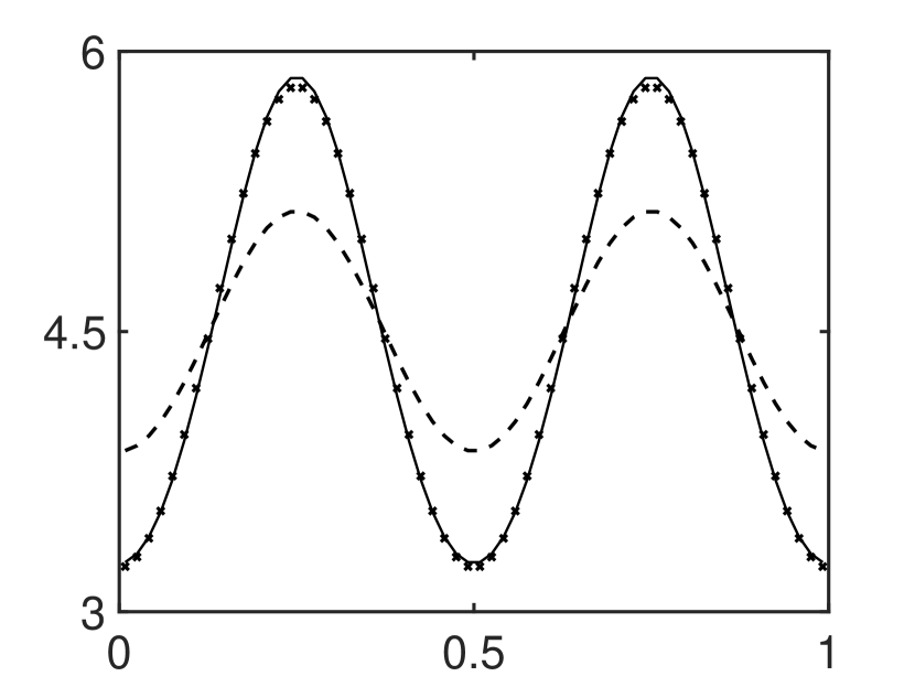
(a) $t=6$

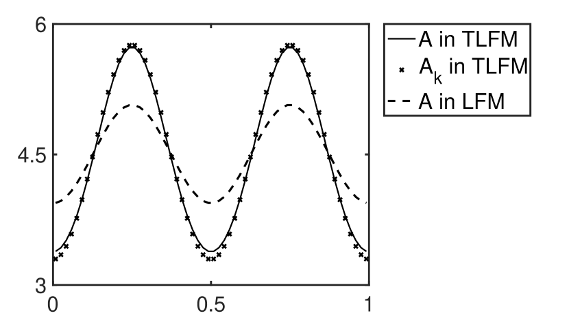
(b) $t=12$

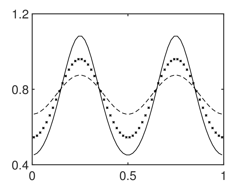
(c) $t=6$

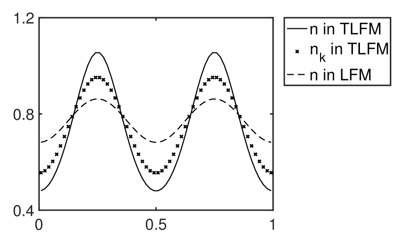
(d) $t=12$

Fig. 3: Comparisons of the discrete and the continuum truncated-Lévy-flight models, and the continuum Lévy-flight model with the equivalent parameters. The plots of the attractiveness field are shown in (a), (b), and those of the criminal number distribution are shown in (c), (d). The discrete model (1)-(5) is shown with cross lines, the continuum truncated-Lévy-flight model (7), (19) is shown with solid lines, and the continuum Lévy-flight model (22) is shown with dashed lines. Here $L=1/l=60$, ${\eta}=0.55$, $\gamma=3.5$, and all the other parameters and data are the same as in Fig. 2. The system enters a steady state at roughly $t=12$.

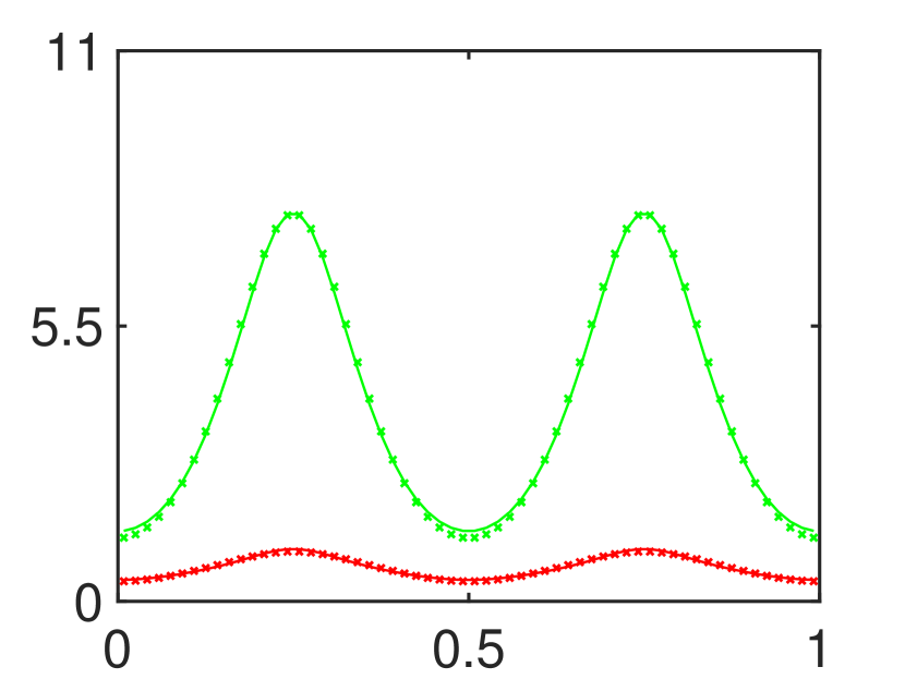
(a) $L=3$

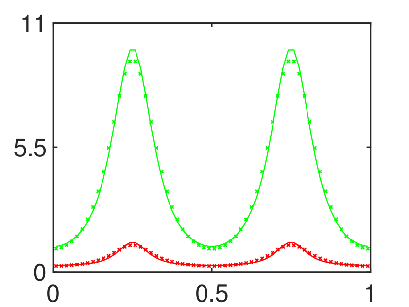
(b) $L=7$

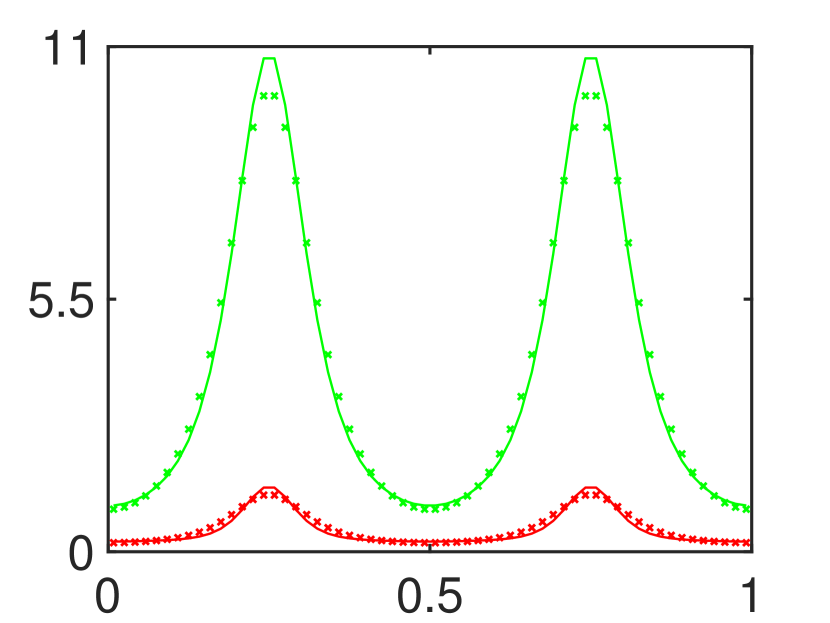
(c) $L=12$

Fig. 4: Comparisons of the discrete and the continuum truncated-Lévy-flight models for different values of $L$. The shots are taken at $t=2$. The discrete model (1)-(5) is shown with the cross lines, and the continuum model (7) and (19) is shown with the solid lines. The plots of the attractiveness field are shown with the green lines, and those of the criminal number distribution are shown with the red lines. Here all the parameters and data are the same as in Fig. 2 except for $\eta=0.12$ and $L$ as indicated.

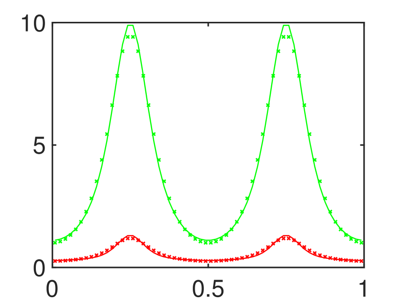
(a) $\mu=1.1$

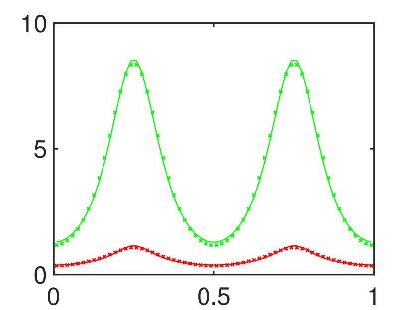
(b) $\mu=2$

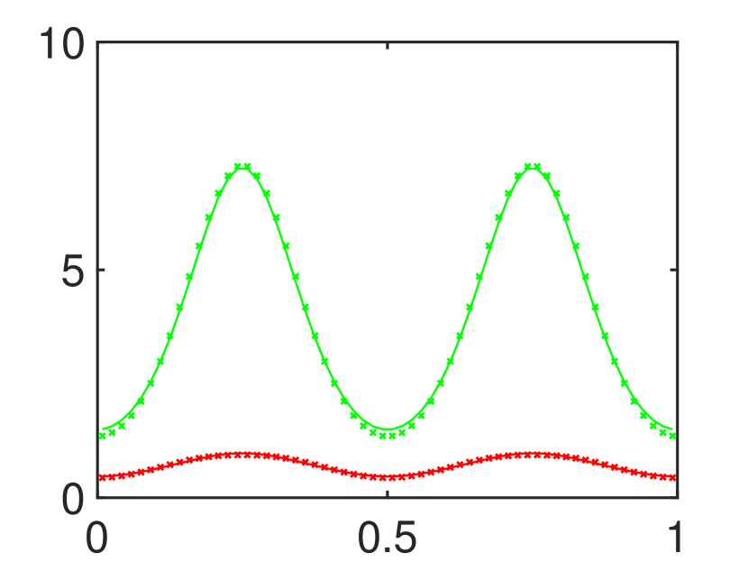
(c) $\mu=2.9$

Fig. 5: Comparisons of the discrete and the continuum truncated-Lévy-flight models for different values of $\mu$. The shots are taken at $t=2$. The discrete model (1)-(5) is shown with the cross lines, and the continuum model (7) and (19) is shown with the solid lines. The plots of the attractiveness field are shown with the green lines, and those of the criminal number distribution are shown with the red lines. Here all the parameters and data are the same as in Fig. 2 except for $\eta=0.12$, $L=3$, and $\mu$ as indicated.

3.3 Linear stability analysis

In this section, we analyze the formation of the hotspots (spatial-temporal collections of criminal activities) as observed in the previous simulations and develop a stability condition. Since the continuum equations (7) and (19) are very similar to (21)₁ and (21)₂, except for a modified diffusion coefficient, the previous stability analysis for the random-walk model (see e.g. (3.21) in Ref. uclaModel) can be extended directly to suit for the truncated-Lévy-flight model.

As in Refs. uclaModel and levycrime, we first rescale the variables in the continuum equations:

$$A={A}^{\ast}\omega,\quad{n}=\dfrac{{{n}}^{\ast}\omega}{\theta},\quad t=\dfrac{{t}^{\ast}}{\omega},\quad{\eta}^{\ast}=\dfrac{l^{2}\eta}{2\omega\delta t}.$$ (25)

Applying (25) to (7) and (19), we obtain (the $\ast$’s are omitted)

$$\displaystyle\dfrac{\partial A}{\partial t} =\eta A_{xx}-A+\alpha+A{{n}},$$ (26)

$$\dfrac{\partial{n}}{\partial t} =\bar{\mathcal{D}}\vec{\nabla}\cdot\left[\vec{\nabla}{n}-\dfrac{2{n}}{A}\vec{\nabla}A\right]-A{{n}}+\beta,$$ (27)

where

$$\bar{\mathcal{D}}=\dfrac{l^{2}}{\delta t}\frac{z^{\ast}_{\mu,L}}{\omega z_{\mu,L}},\hskip 14.22636pt\alpha=\dfrac{A^{0}}{\omega},\hskip 14.22636pt\beta=\dfrac{\gamma\theta}{\omega^{2}}.$$ (28)

Let the steady states be $(\bar{A},\bar{{{n}}})$,

$$\bar{A}=\alpha+\beta,\qquad\bar{{{n}}}=\dfrac{\beta}{\alpha+\beta}.$$ (29)

We find the following stability conditions of the system around the homogeneous steady states:

Theorem 3.2.

When $\bar{{{n}}}<1/3$, the homogeneous equilibrium in (29) is stable. When $\bar{{{n}}}>1/3$, the equilibrium is unstable if

$$\eta<\bar{\mathcal{D}}\dfrac{3\bar{{{n}}}+1-\sqrt{12\bar{{{n}}}}}{\bar{A}}.$$ (30)

Proof 3.3.

The proof is very similar to that in Ref. uclaModel, that is, we apply a linear Turing stability analysis on (26) and (27) around the homogeneous steady state. We decompose the solutions as perturbations from the steady states:

$$A(x,t)=\bar{A}+\delta_{A}e^{\sigma t}e^{ikx},\quad{{n}}(x,t)=\bar{{{n}}}+\delta_{{n}}e^{\sigma t}e^{ikx}.$$ (31)

Substituting (31) into (26) and (27), we obtain

$$\begin{bmatrix}-\eta|k|^{2}-1+\bar{{{n}}}&\bar{A}\\ \dfrac{2\bar{{{n}}}}{\bar{A}}\bar{\bar{\mathcal{D}}}|k|^{2}-\bar{{{n}}}&-\bar{\mathcal{D}}|k|^{2}-\bar{A}\end{bmatrix}\begin{bmatrix}\delta_{A}\\ \delta_{{n}}\end{bmatrix}=\sigma\begin{bmatrix}\delta_{A}\\ \delta_{{n}}\end{bmatrix}.$$ (32)

We solve for the eigenvalue problem (32). We first rewrite it as

$$\begin{bmatrix}-\eta|k|^{2}-1+\bar{{{n}}}-\sigma&\bar{A}\\ \dfrac{2\bar{{{n}}}}{\bar{A}}\bar{\mathcal{D}}|k|^{2}-\bar{{{n}}}&-\bar{\mathcal{D}}|k|^{2}-\bar{A}-\sigma\end{bmatrix}\begin{bmatrix}\delta_{A}\\ \delta_{{n}}\end{bmatrix}=0.$$ (33)

Setting the determinant of the square matrix on the left-hand-side as zero, we obtain

$$\sigma^{2}-\tau\sigma+\delta=0,$$ (34)

where

$$\tau =-\bar{\mathcal{D}}|k|^{2}-\eta|k|^{2}-\bar{A}-1+\bar{{{n}}},$$ (35)

$$\delta =\bar{\mathcal{D}}|k|^{2}(\eta|k|^{2}+1-3\bar{{{n}}})+\eta|k|^{2}\bar{A}+\bar{A}.$$ (36)

The equilibrium is stable if both solutions to (34) have negative real parts. Since $\alpha,\beta>0$, thus $\bar{A}>0,0<\bar{{{n}}}<1$, we observe that $\tau\leq 0$. Therefore, the equilibrium is stable if $\delta>0$. We then observe that if $\bar{{{n}}}<1/3$, then $\delta>0$. It follows that the equilibrium is stable when $\bar{{{n}}}<1/3$.

Now we consider the case when $\bar{{{n}}}>1/3$. Since the equilibrium is unstable if $\delta<0$, from (36) we rewrite the condition $\delta<0$ equivalently as

$$\bar{A}<\bar{\mathcal{D}}|k|^{2}\Bigg{(}-1+\dfrac{3\bar{{{n}}}}{\eta|k|^{2}+1}\Bigg{)},\quad\forall k.$$ (37)

Setting $x=\eta|k|^{2}$, from (37) we infer

$$\bar{A}<\max_{x\geq 0}\left[\bar{\mathcal{D}}\eta^{-1}x\Bigg{(}-1+\dfrac{3\bar{{{n}}}}{x+1}\Bigg{)}\right].$$ (38)

To calculate the right-hand side of (38), we set the derivative of the corresponding function in $x$ equal to zero, and arrive at

$$\bar{\mathcal{D}}\eta^{-1}\dfrac{-3\bar{{n}}x}{(x+1)^{2}}+\bar{\mathcal{D}}\eta^{-1}(-1+\dfrac{3\bar{{{n}}}}{x+1})=0,$$

$$x^{2}+2x+1-3\bar{{{n}}}=0.$$ (39)

We substitute the positive root $x=-1+\sqrt{3\bar{{n}}}$ into (38) and obtain

$$\bar{A}<\bar{\mathcal{D}}\eta^{-1}(-1+\sqrt{3\bar{{{n}}}})^{2}.$$ (40)

This together with (37) implies (30) as desired.

4 Incorporation of Law Enforcement Agents

In the field there is another essential component that affects the criminal behavior, namely, the presence of law enforcement agents. We incorporate their effects into the truncated-Lévy-flight model. We assume that the law enforcement agents also follow truncated Lévy flights, whose mobility parameters are possibly different than those of the criminal agents. These parameters will determine their deployment strategy. We study the effects these law enforcement agents have on the formation of the hotspots and total number of criminal activities, and how they depend on the mobility parameters quantitatively and qualitatively. In Ref. law_enforcement, only qualitative comparisons were carried out. In Ref. Zipkin law enforcement agents were also incorporated but the focus was on the optimization of the deployment strategy through the study of a free boundary problem.

4.1 Discrete model

Let $\psi_{k}(t)$ be the number of the law enforcement agents at site $k$ at time $t$, and $\tilde{A_{k}}(t)$ be the attractiveness perceived by the criminals in the presence of the police agents. As in Ref. law_enforcement, we assume that

$$\tilde{A_{k}}(t):=e^{-\chi\psi_{k}(t)}A_{k}(t),$$ (41)

where $\chi$ is a given constant measuring the effectiveness of the patrol strategy. Now we modify the model to include the effects of the law enforcement agents. The probability of burglarizing and moving of the criminal agents are the same as in Section 2.1, except for $\tilde{A}$ replacing $A$. Thus at each time step, the system gets updated as follows:

Step 1. Each criminal agent decides to burglarize with probability

$$\tilde{p}_{k}(t)=1-e^{-\tilde{A}_{k}(t)\delta t}.$$ (42)

Step 2. If a criminal agent chooses to commit a burglary then he will be immediately removed from the system. Otherwise he will move from site $k$ to site $i$ with probability

$$\tilde{q}_{k\rightarrow i}(t)=\dfrac{\tilde{w}_{k\rightarrow i}(t)}{\sum\limits_{\begin{subarray}{c}j\in\mathbb{Z}\\ j\neq k\end{subarray}}{\tilde{w}_{k\rightarrow j}(t)}},\quad k\neq i,$$ (43)

where

$$\tilde{w}_{k\rightarrow i}(t)=\left\{\begin{array}[]{@{}c@{\quad}l@{}}\dfrac{\tilde{A}_{i}(t)}{l^{\mu}|i-k|^{\mu}},&1\leq|i-k|\leq L,\\ 0,&\text{otherwise}.\end{array}\right.$$ (44)

Step 3. The law enforcement agents move following a truncated Lévy flight biased according to the original attractiveness field. Hence the probability of a law enforcement agent moving from site $k$ to site $i$ is

$$\widehat{q}_{k\rightarrow i}(t)=\dfrac{\widehat{w}_{k\rightarrow i}(t)}{\sum\limits_{\begin{subarray}{c}j\in\mathbb{Z}\\ j\neq k\end{subarray}}{\widehat{w}_{k\rightarrow j}(t)}},\quad k\neq i,$$ (45)

where

$$\widehat{w}_{k\rightarrow i}(t)=\left\{\begin{array}[]{lr}\dfrac{A_{i}(t)}{l^{\widehat{\mu}}|i-k|^{\widehat{\mu}}},&1\leq|i-k|\leq\widehat{L},\\ 0,&\text{otherwise}.\end{array}\right.$$ (46)

Here $\widehat{\mu}\in(1,3)$ and $\widehat{L}\in\mathbb{N}$. These mobility parameters of the law enforcement agents are not necessarily the same with those of the criminal agents. We also demand that the total number of law enforcement agents remains a constant in time; there is no removal or replacement of the police agents.

Step 4. The attractiveness evolves in a way similar to (5) except for a change in the number of burglary events in the time interval $(t,t+\delta t]$. From (42) we infer that there are on average $\delta t\tilde{A_{k}}(t){n}_{k}(t)$ crimes in each time interval on site $k$, and we define the update rule as

$$B_{k}(t+\delta t)=\left[(1-\eta)B_{k}(t)+\dfrac{\eta}{2}(B_{k-1}(t)+B_{k+1}(t))\right](1-\omega\delta t)+\theta\delta t\tilde{A_{k}}(t){n}_{k}(t),$$ (47)

where $\eta$, $\omega$ and $\theta$ are the same parameters as in (5).

Step 5. At each site a new criminal agent is replaced with rate $\gamma$.

Figure 6 presents a visual summary of steps in the form of a flow chat.

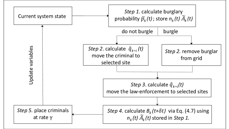
Fig. 6: Flowchart summarizing the discrete model with the incorporation of law enforcement agents.

To conclude, the discrete mean field equation of $(A_{k}(t),\tilde{A}_{k}(t),n_{k}(t),\psi_{k}(t))$ consists of (41), (47), and the following equations

$${n}_{k}(t+\delta t) =\sum_{\begin{subarray}{c}i\in\mathbb{Z}\\ 1\leq|i-k|\leq L\end{subarray}}{[1-\tilde{A}_{i}(t)\delta t]{n}_{i}(t)\tilde{q}_{i\rightarrow k}(t)}+\gamma\delta t,$$ (48)

$$\psi_{k}(t+\delta t) =\sum_{|i-k|\leq\widehat{L}}{\psi_{i}(t)\widehat{q}_{i\rightarrow k}(t)}.$$ (49)

4.2 Continuum model

The derivation of the continuum equations for the attractiveness field and the criminal number distribution is very similar as that in Sec. 3; basically, from (47) and (48) we obtain (7) and (19) with $A$ replaced by $\tilde{A}$ when suitable:

$$\dfrac{\partial A}{\partial t} =\dfrac{l^{2}\eta}{2\delta t}A_{xx}-\omega(A-A^{0})+\theta{n}\tilde{A},$$ (50)

$$\dfrac{\partial{n}}{\partial t} =\mathcal{D}\vec{\nabla}\cdot\left[\vec{\nabla}{n}-\dfrac{2{n}}{\tilde{A}}\vec{\nabla}\tilde{A}\right]-\tilde{A}{n}+\gamma.$$ (51)

This however will not lead to the identical system since now (50) and (51) are part of a larger system which also includes the dynamics of the component of law enforcement agent. With a similar derivation as in Sec. 3, from (49) we obtain

$$\dfrac{\partial\psi}{\partial t}=\widehat{\mathcal{D}}\vec{\nabla}\cdot\left[\vec{\nabla}\psi-\dfrac{2\psi}{A}\vec{\nabla}A\right],$$ (52)

where

$$\widehat{\mathcal{D}}=\dfrac{l^{2}}{\delta t}\dfrac{z^{\ast}_{\widehat{\mu},\widehat{L}}}{z_{\widehat{\mu},\widehat{L}}}.$$ (53)

To conclude, the continuum model with law enforcement effects consists of (41) and (50)-(52).

4.3 Computer simulations

In order to verify the validity of our continuum model, and to compare results with the discrete model, we perform direct numerical simulations. We consider the basic deployment strategies including a biased random walk (BRW) and a truncated Lévy flight (TLF) with the same mobilities as those of the criminal agents. As in Ref. law_enforcement, we also include the base case where the law enforcement agents patrol random routes, that is, an unbiased random walk (URW). Here the law enforcement agents do not focus their attention on any particular place. In this case, the continuum equation for the dynamics of law enforcement agents is just the unbiased Brownian motion. [6]

To implement the discrete model, we consider a lattice grid on a spatial domain $[0,1]$ with the lattice spacing being ${l}=1/60$. The computation assumes periodic boundary conditions. The algorithm used for the continuum simulation is very similar to that used in Section 3.2. Particularly, we use a semi-implicit time discretization, with the time-stepping algorithms as follows:

$$\tilde{A}^{(m)} =A^{(m)}e^{-\chi\psi^{(m)}},$$ (54)

$$A^{(m+1)} =A^{(m)}+\Delta t\left(\eta A_{xx}^{(m)}-A^{(m)}+A^{0}+n^{(m)}\tilde{A}^{(m)}\right),$$ (55)

$$n^{(m+1)} =n^{(m)}+\mathcal{D}\Delta t\left[n^{(m)}_{xx}-\left(\dfrac{2n\tilde{A}_{x}^{(m+1)}}{\tilde{A}^{(m+1)}}\right)_{x}\right]+\Delta t\left(-\tilde{A}^{(m+1)}n^{(m)}+\gamma\right),$$ (56)

$$\psi^{(m+1)} =\psi^{(m)}+\hat{\mathcal{D}}\Delta t\left[\psi^{(m)}_{xx}-\left(\frac{2\psi^{(m)}A^{(m+1)}_{x}}{A^{(m+1)}}\right)_{x}\right].$$ (57)

Here $f^{(m)}$ represents a quantity $f$ at $m$th time step. To discretize the functional space of the solutions, we use the fast Fourier transform (FFT).

Figs. 7, 8, and 9 below show the discrete and the continuum models corresponding to the three deployment strategies. Good agreement is observed in all cases, which validates the continuum models. It is expected that the unbiased random walk in Fig. 7 does not reduce hotspot activity and is the least effective of all the three strategies, which agrees with the empirical evidence in Ref. law_enforcement. However the comparison of Fig. 8 and Fig. 9 is less trivial. It seems that Fig. 9 shows higher deployment effectiveness, as a steady state is reached faster. However for a better comparison we need to first quantify the effectiveness of the deployment strategies.

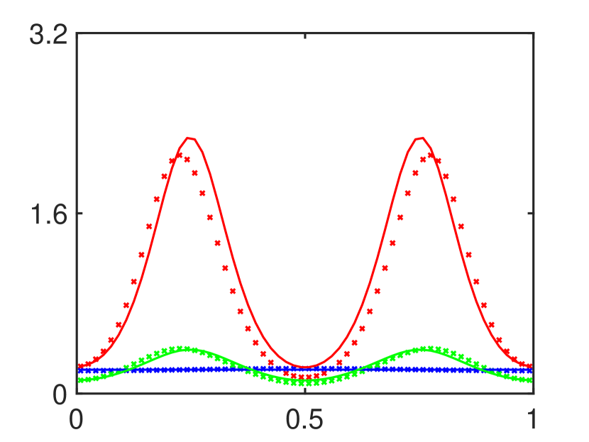
(a) $t=5$

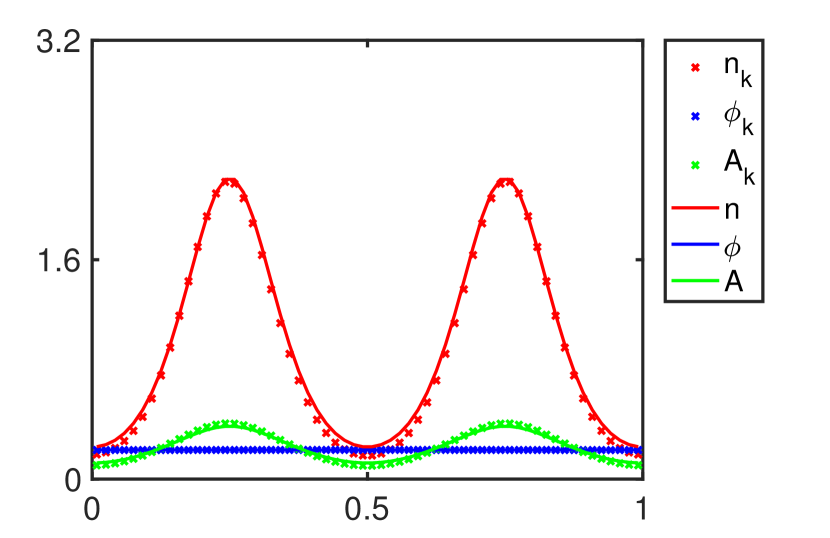
(b) $t=10$

Fig. 7: Comparisons of the discrete and the continuum models with the unbiased-random-walk deployment strategy. The discrete model (41)-(47) is shown with cross lines, and the continuum model (41) and (50)-(52) is shown with solid lines. The attractiveness field, the criminal and the law enforcement agent number distributions are shown with green, red and blue lines. The initial conditions (at $t=0$) are taken to be $\psi=1/3\sin(\pi x)$, $B\equiv 0$ and ${{n}}=1-0.3\cos(4\pi x)$. Parameters are $\chi=8$, $A^{0}=1-0.5\cos(4\pi x)$, $l=1/60$, $\delta t=0.01$, $L=9$, ${\eta}=0.1$, $\gamma=0.3$, $\omega=1$, $\theta=1$, and $\widehat{L}=1$. The system enters a steady state at roughly $t=10$.

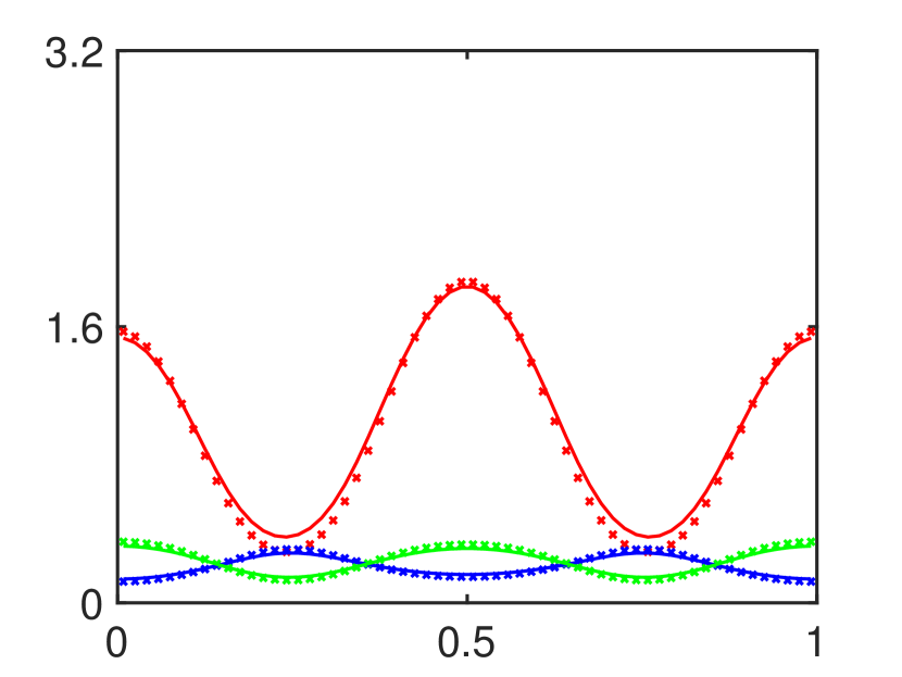
(a) $t=5$

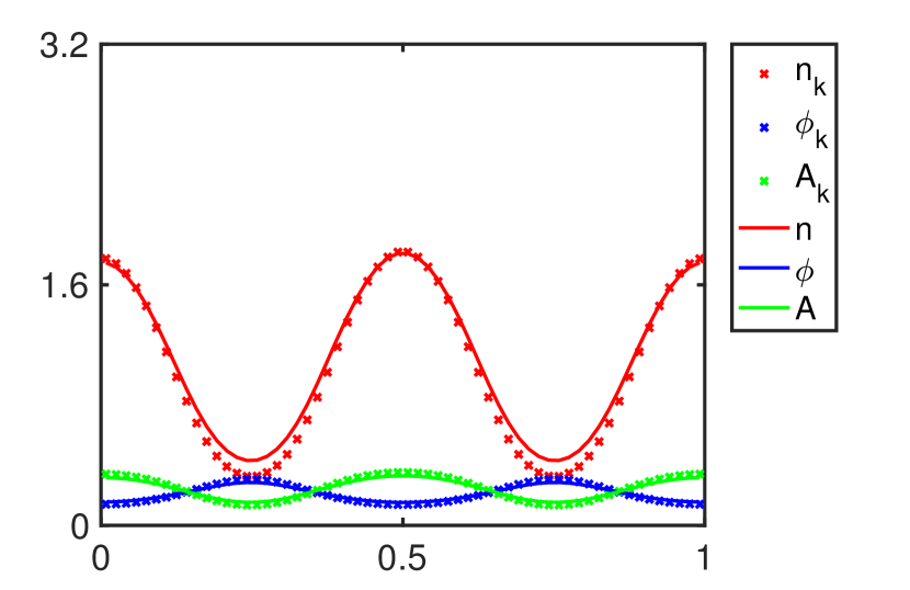
(b) $t=10$

Fig. 8: Comparisons of the discrete and the continuum models with a biased-random-walk deployment strategy. All the parameters and data are the same as in Fig. 7. The system enters a steady state roughly at $t=10$.

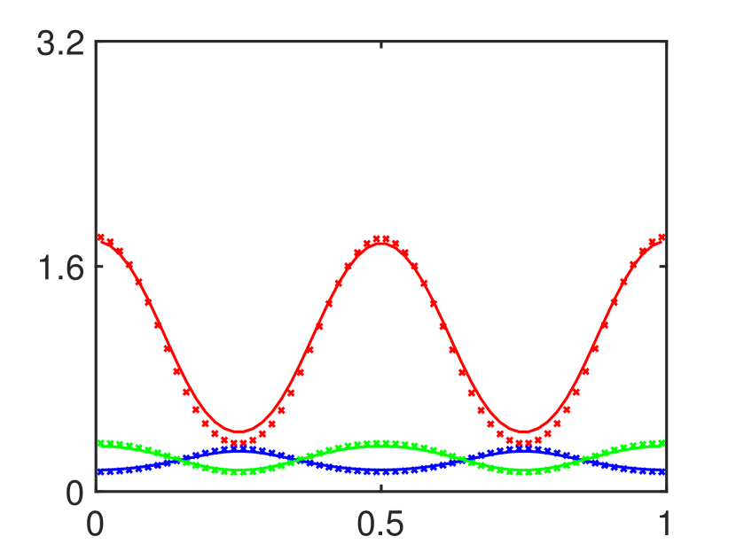
(a) $t=5$

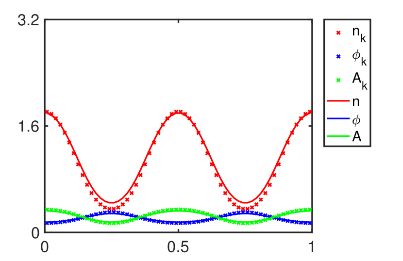
(b) $t=10$

Fig. 9: Comparisons of the discrete and the continuum models when the deployment strategy of a truncated Lévy flight is adopted. Here $\widehat{L}=L=9$, $\widehat{\mu}=\mu=2.5$, and all the other parameters and data are the same as in Fig. 7. The system enters a steady state roughly at $t=5$.

Remark 4.1.

In Ref. law_enforcement, a “peripheral interdiction” was also considered, which sends the police to the perimeters of the crime hotspots instead of the centers. However this deployment strategy is not considered here, as the criminals can take long jumps now, and protecting the perimeters of a hotspot no longer necessarily prevents them from entering the center.

4.4 Quantitative comparisons of the patrol effectiveness

We compute the cumulative number of burglaries for the system. From (42) we infer that the total expected number of burglary events over the whole domain up to time $T$ equals to $\sum_{k}\sum_{t=n\delta t,\,\,\,0<t<T}{\tilde{A_{k}}(t){n}_{k}(t)\delta t}$, where $k$ is sum over all the grid points in the domain. When the domain size is kept fixed and $l$ is sent to zero, the total number of grid points in this domain will increase to infinity. Therefore, to make sense of the above quantity, we rescale it by multiplying it with $l$, and physically it means the averaged expected number of burglaries. Then taking the limit as $\delta t$ and $l$ become small, the rescaled double sum yields a double integral, denoted as $S(T)$:

$$S(T)=\int_{0}^{T}\int_{\mathcal{M}}{\tilde{A}(x,t){{n}}(x,t)dxdt},$$ (58)

where $\mathcal{M}$ denotes the spatial domain on which the lattice grid lives. The instantaneous global crime rate can be defined as

$$R(t):=\dfrac{\partial S(t)}{\partial t}=\int_{\mathcal{M}}{\tilde{A}(x,t){{n}}(x,t)dx}.$$ (59)

Fig. 10 below shows the simulations of $R(t)$ and $S(t)$ when zero law enforcement agent is put in the system, and when one of the deployment strategies mentioned in Section 4.3 above are employed, that is, an unbiased and a biased random walk, and a truncated Lévy flight with the same mobility parameters as the criminals.

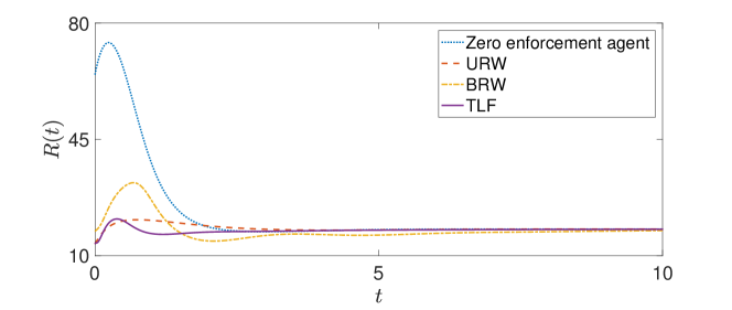
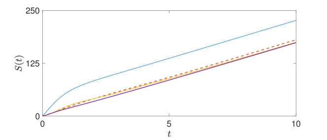
Fig. 10: Output of $R(t)$ and $S(t)$, when there is no law enforcement agent, and when the deployment strategy of an unbiased random walk (URW), a biased random walk (BRW), or a truncated Lévy flight (TLF) is adopted. Here all the parameters and data are the same as in Figs. 7-9, except for $l=1$ and the spatial domain $\mathcal{M}=[0,60]$.

We observe that $R(t)$ approaches a constant steady state independent of the incorporation of law enforcement agents. In fact, we find that this steady state only depends on the rate of criminals entering the system and the size of the domain:

Theorem 4.2.

Once the system (41) and (50)-(52) is in a steady state at time $T$, we have

$$R(t)=\gamma|\mathcal{M}|,\quad\forall t\geq T,$$ (60)

where $|\mathcal{M}|$ is the size of the domain $\mathcal{M}$.

Proof 4.3.

We integrate (51) over the domain $\mathcal{M}$

$$\dfrac{\text{d}}{\text{d}t}\int_{\mathcal{M}}{{n}}\,dx =\int_{\mathcal{M}}{{{n}}_{t}}\,dx$$

$$={\mathcal{D}}\int_{\mathcal{M}}\left[\tilde{A}\left(\dfrac{{{n}}}{\tilde{A}}\right)_{xx}-\dfrac{{{n}}}{\tilde{A}}\tilde{A}_{xx}\right]-\tilde{A}{{n}}+\gamma\,dx$$

$$={\mathcal{D}}\left[\tilde{A}(\dfrac{{{n}}}{\tilde{A}})_{x}-\dfrac{{{n}}}{\tilde{A}}\tilde{A}_{x}\right]\bigg{|}_{\mathcal{M}}-\int_{\mathcal{M}}{(\tilde{A}{{n}}-\gamma)\,dx}$$

$$=\gamma|\mathcal{M}|-\int_{\mathcal{M}}\tilde{A}{{n}}\,dx.$$ (61)

Here the periodic boundary conditions are applied. When the system is at a steady state, the left-hand-side of (61) vanishes, and hence (60) follows as desired.

In the original random-walk model [38] the crime suppression was built-in to the decay of the attractiveness. This was used to model the finite lifetime of the repeat victimization effect. Here we add additional law enforcement who curb the crimes by decreasing the attractiveness. We noted that in Fig. 10 with or without law enforcement agents the steady state crime rate is identical. This happens essentially because of the constant replacement rate, and was first observed in the original random-walk model. [38] Nevertheless, Fig. 10 shows that law enforcement agents do affect the number of burglary events cumulated before the crime rate enters the steady state. Thus it seems reasonable to measure the deployment efficiency using $S(T)$ at the time $T$, when $R(T)$ just enters the equilibrium. In Fig. 10, $T$ can be chosen as $5$, as $R(T)$ is always within negligible difference from the steady state crime rate after time $5$.

Tables 1, 2 and 3 below display $S(5)$ for the three deployment strategies shown in Fig. 10 (the system enters the steady state roughly at $T=5$ in all three cases). We observe from these tables that the truncated Lévy flight with the same mobility parameters as the criminals is the most effective deployment strategy in terms of reducing the total number of crime events. This quantitative result coincides with our intuition and the qualitative comparisons in Figs. 7-9.

Table 1: Comparisons of the global cumulative number of the burglary events till time $T=5$ between different deployment strategies. ‘Improvement I’ shows the improvement compared to the base case with zero enforcement agents. ‘Improvement II’ corresponds to the improvement compared to the unbiased-random-walk deployment strategy. The parameters and initial conditions are the same as in Fig. 10. In this case there are initially two regions of high attractiveness.

The Police Deployment Strategy	S(5)	Improvement I	Improvement II
Zero Law Enforcement Agent	137	-	-
Unbiased Random Walk	91.87	32.94$\%$	-
Biased Random Walk	88.91	35.1$\%$	3.22$\%$
Truncated Lévy Flight	85.26	37.76$\%$	7.19$\%$

Table 2: Comparisons of the global cumulative number of the burglary events till time $T=5$ between different deployment strategies. Here the initial conditions (at $t=0$) are taken to be ${{n}}=1-0.3\cos(8\pi x)$ and $A^{0}=1-0.5\cos(8\pi x)$, and all the other parameters and data are the same as in Table 1. In this case, there are four regions of high attractiveness initially.

The Police Deployment Strategy	S(5)	Improvement I	Improvement II
Zero Law Enforcement Agent	136.46	-	-
Unbiased Random Walk	97.83	28.3$\%$	-
Biased Random Walk	85.69	37.2$\%$	12.41$\%$
Truncated Lévy Flight	82.73	39.37$\%$	15.44$\%$

Table 3: Comparisons of the global cumulative number of the burglary events till time $T=5$ between different deployment strategy. Here the initial conditions are taken to be ${{n}}=1-0.3\cos(16\pi x)$ and $A^{0}=1-0.5\cos(16\pi x)$, and all the other parameters and data are the same as in Table 1. In this case, there are eight regions of high attractiveness initially.

The Police Deployment Strategy	S(5)	Improvement I	Improvement II
Zero Law Enforcement Agent	136.4	-	-
Unbiased Random Walk	102.74	24.68$\%$	-
Biased Random Walk	83.11	39.07$\%$	19.1$\%$
Truncated Lévy Flight	79.2	41.93$\%$	22.91$\%$

5 Conclusion

In this paper, we apply the truncated Lévy flights to the class of agent-based crime models for residential burglary. The truncation becomes a parameter that restricts the mobility of the agents. We study both the discrete model and its continuum limit which agree very well in computer simulations. We find that the continuum system behaves like modified Brownian dynamics. This indicates that the continuum version of the original random-walk model in Ref. uclaModel, which also has a Brownian dynamics, can be utilized here with a modified diffusion coefficient. For instance, the stability analysis in the original paper [38] can be modified and applied to our model efficiently. This serves as a first step towards the weakly nonlinear analysis and bifurcation theory which can help law-enforcement to understand the feedback between treatment and hotspot dynamics. [36, 34]. Then we examine the impact of introducing police into the truncated-Lévy-flight model, whose mobility parameters determine the deployment strategies. We observe that the strategies can affect the global cumulative number of the burglary events before the system steady state is reached. We make a quantitative comparison of the deployment strategy efficiency accordingly. We find that the truncated Lévy flight with the same mobility parameters as those of the criminal agents is the most efficient, compared to the deployment strategies of an unbiased and a biased random walk.

For the future work, on the one hand, we can extend the truncated-Lévy-flight model to two dimensional-space, which is more realistic when modeling household distributions in typical urban area. Then we can explore whether the “finite size effects” observed previously in the original model [38] is also an attribution of our model, namely, whether the transience of the hotspot dynamics in the discrete simulations will depend on the initial population size. On the other hand, we can continue the study of the dependence of the law enforcement patrol efficiency upon the mobility parameters of the agents. A complete parametrization of the efficiency with the mobility parameters may be suggestive for the police patrol strategy design.

References

- [1] N. Bellomo, F. Colasuonno, D. Knopoff and J. Soler, From a systems theory of sociology to modeling the onset and evolution of criminality, Netw. Het. Media 10 (2015) 421–441.
- [2] H. Berestycki, N. Rodríguez and L. Ryzhik, Traveling wave solutions in a reaction-diffusion model for criminal activity, Multiscale Model. Simul. 11 (2013) 1097–1126.
- [3] D. Brockmann, L. Hufnagel and T. Geisel, The scaling laws of human travel, Nature 439 (2006) 462–465.
- [4] T. Budd, Burglary of domestic dwellings: Findings from the British Crime Survey, Home Office Statistical Bulletin 4 (1999).
- [5] L. Cao and M. Grabchak, Smoothly truncated levy walks: Toward a realistic mobility model, 2014 IEEE 33rd International Performance Computing and Communications Conference (IPCCC) (2014) 1–8.
- [6] S. Chaturapruek, J. Breslau, D. Yazdi, T. Kolokolnikov and S. G. McCalla, Crime modeling with Lévy flights, SIAM J. Appl. Math. 73 (2013) 1703–1720.
- [7] G. Farrell and K. Pease, Repeat Victimization, Criminal Justice Press, Monsey, New York, 2001.
- [8] J. M. Gau and T. C. Pratt, Revisiting broken windows theory: Examining the sources of the discriminant validity of perceived disorder and crime, Journal of Criminal Justice 38 (2010) 758–766.
- [9] M. C. González, C. A. Hidalgo and A.-L. Barabási, Understanding individual human mobility patterns, Nature 453 (2008) 779–782.
- [10] W. Gorr and Y. Lee, Early warning system for temporary crime hot spots, J. Quantitative Criminology 31 (2015) 25–47.
- [11] T. Goudon, B. Nkonga, M. Rascle and M. Ribot, Self-organized populations interacting under pursuit-evasion dynamics, Phys. D 304/305 (2015) 1–22.
- [12] B. E. Harcourt, Reflecting on the subject: A critique of the social influence conception of deterrence, the broken windows theory, and order-maintenance policing New York style, Michigan Law Review 97 (1998) 291–389.
- [13] A. James, M. J. Plank and A. M. Edwards, Assessing Lévy walks as models of animal foraging, J. R. Soc. Interface 8 (2011) 1233–1247.
- [14] S. D. Johnson, W. Bernasco, K. J. Bowers, H. Elffers, J. Ratcliffe, G. Rengert and M. Townsley, Space-time patterns of risk: A cross national assessment of residential burglary victimization, J. Quantitative Criminology 23 (2007) 201–219.
- [15] S. D. Johnson and K. J. Bowers, The stability of space-time clusters of burglary, Brit. J. Criminol. 44 (2004) 55–65.
- [16] S. D. Johnson, K. Bowers and A. Hirschfield, New insights into the spatial and temporal distribution of repeat victimization, Brit. J. Criminol. 37 (1997) 224–241.
- [17] P. A. Jones, P. J. Brantingham and L. R. Chayes, Statistical models of criminal behavior: the effects of law enforcement actions, Math. Models Methods Appl. Sci. 20 (2010) 1397–1423.
- [18] T. Kolokolnikov, M. J. Ward and J. Wei, The stability of steady-state hot-spot patterns for a reaction-diffusion model of urban crime, Discrete Contin. Dyn. Syst. Ser. B 19 (2014) 1373–1410.
- [19] P. J. van Koppen and R. W. J. Jansen, The road to the robbery: Travel patterns in commercial robberies, Brit. J. Criminol. 38 (1998) 230–246.
- [20] T. Levajković, H. Mena and M. Zarfl, Lévy processes, subordinators and crime modeling, Novi Sad J. Math. 46 (2016) 65–86.
- [21] D.J.B. Lloyd and H. O’Farrell, On localised hotspots of an urban crime model, Phys. D 253 (2013) 23–39.
- [22] R. N. Mantegna and H. E. Stanley, Stochastic process with ultraslow convergence to a Gaussian: the truncated Lévy flight, Phys. Rev. Lett. 73 (1994) 2946–2949.
- [23] M. C. Mariani and Y. Liu, Normalized truncated Levy walks applied to the study of financial indices, Physica A: Statistical Mechanics and its Applications 377 (2007) 590–598.
- [24] G. Ajmone Marsan, N. Bellomo and L. Gibelli, Stochastic evolutionary differential games toward a systems theory of behavioral social dynamics, Math. Models Methods Appl. Sci. 26 (2016) 1051–1093.
- [25] A. Matacz, Financial modeling and option theory with the truncated Lévy process, Int. J. Theor. Appl. Finan. 3 (2000) 143–160.
- [26] S. G. McCalla, M. B. Short and P. J. Brantingham, The effects of sacred value networks within an evolutionary, adversarial game, J. Stat. Phys. 151 (2013) 673–688.
- [27] L. C. Miranda and R. Riera, Truncated Lévy walks and an emerging market economic index, Physica A: Statistical Mechanics and its Applications 297 (2001) 509–520.
- [28] G. O. Mohler, M. B. Short, P. J. Brantingham, F. P. Schoenberg, and G. E. Tita, Self-exciting point process modeling of crime, J. Amer. Statist. Assoc. 106 (2011) 100–108.
- [29] G. O. Mohler, M. B. Short, S. Malinowski, M. Johnson, G. E. Tita, A. L. Bertozzi and P. J. Brantingham, Randomized controlled field trials of predictive policing, J. Amer. Statist. Assoc. 110 (2015) 1399–1411.
- [30] G. O. Mohler, M. B. Short and P. J. Brantingham, The concentration-dynamics tradeoff in crime hot spotting, Unraveling the Crime-Place Connection 22 (2017) 19-40.
- [31] A. B. Pitcher, Adding police to a mathematical model of burglary, European J. Appl. Math. 21 (2010) 401–419.
- [32] N. Rodríguez, On the global well-posedness theory for a class of PDE models for criminal activity, Phys. D 260 (2013) 191–200.
- [33] N. Rodríguez and A. L. Bertozzi, Local existence and uniqueness of solutions to a PDE model for criminal behavior, Math. Models Methods Appl. Sci. 20 (2010) 1425–1457.
- [34] M. B. Short, A. L. Bertozzi and P. J. Brantingham, Nonlinear patterns in urban crime: hotspots, bifurcations, and suppression, SIAM J. Appl. Dyn. Syst. 9 (2010) 462–483.
- [35] M. B. Short, G. O. Mohler, P. J. Brantingham and G. E. Tita, Gang rivalry dynamics via coupled point process networks, Discrete Contin. Dyn. Syst. Ser. B 19 (2014) 1459–1477.
- [36] M. B. Short, P. J. Brantingham, A. L. Bertozzi and G. E. Tita, Dissipation and displacement of hotspots in reaction-diffusion models of crime, Proc. Natl. Acad. Sci. 107 (2010) 3961–3965.
- [37] M. B. Short, M. R. D’Orsogna, P. J. Brantingham and G. E. Tita, Measuring and modeling repeat and near-repeat burglary effects, J. Quantitative Criminology 25 (2009) 325–339.
- [38] M. B. Short, M. R. D’Orsogna, V. B. Pasour, G. E. Tita, P. J. Brantingham, A. L. Bertozzi and L. B. Chayes, A statistical model of criminal behavior, Math. Models Methods Appl. Sci. 18 (2008) 1249–1267.
- [39] B. Snook, Individual differences in distance travelled by serial burglars, J. Investig. Psych. Offender Profil. 1 (2004) 53–66.
- [40] W. H. Tse and M. J. Ward, Hotspot formation and dynamics for a continuum model of urban crime, European J. Appl. Math. 27 (2016) 583–624.
- [41] J. Q. Wilson and G. L. Kelling, Broken windows: The police and neighborhood safety, Atlantic Mon. 249 (1982) 29–38.
- [42] J. R. Zipkin, M. B. Short and A. L. Bertozzi, Cops on the dots in a mathematical model of urban crime and police response, Discrete Contin. Dyn. Syst. Ser. B 19 (2014) 1479–1506.