Entanglement in correlated random spin chains, RNA folding and kinetic roughening

Abstract

Average block entanglement in the 1D XX-model with uncorrelated random couplings is known to grow as the logarithm of the block size, in similarity to conformal systems. In this work we study random spin chains whose couplings present long range correlations, generated as gaussian fields with a power-law spectral function. Ground states are always planar valence bond states, and their statistical ensembles are characterized in terms of their block entropy and their bond-length distribution, which follow power-laws. We conjecture the existence of a critical value for the spectral exponent, below which the system behavior is identical to the case of uncorrelated couplings. Above that critical value, the entanglement entropy violates the area law and grows as a power law of the block size, with an exponent which increases from zero to one. Similar planar bond structures are also found in statistical models of RNA folding and kinetic roughening, and we trace an analogy between them and quantum valence bond states. Using an inverse renormalization procedure we determine the optimal spin-chain couplings which give rise to a given planar bond structure, and study the statistical properties of the couplings whose bond structures mimic those found in RNA folding.

I Introduction

Entanglement in disordered spin chains has received much attention recently Refael.04 ; Laflorencie.05 ; Hoyos.07 ; Ramirez.14 . The main reason is that, as opposed to on-site disordered systems Anderson.58 , long-distance correlations are not destroyed in this case, but only modified in subtle ways. Thus, for the 1D Heisenberg and XX models with uncorrelated random couplings, the von Neumann entropy of blocks of size $\ell$ is known to violate the area law and grow as $\log(\ell)$, similarly to the conformal case Vidal.03 ; Eisert.10 . The prefactor, nonetheless, is different: it is still proportional to the the central charge of the associated conformal field theory (CFT), but multiplied by an extra $\log(2)$ factor. Moreover, the Rényi entropies do not satisfy the predictions of CFT Cardy.09 , because these models are not conformal invariant.

A very relevant tool of analysis is the strong disorder renormalization group (SDRG) devised by Dasgupta and Ma Dasgupta.80 , which shows that the ground state of Heisenberg or XX chains with strong disorder can be written as a product of random singlets, in which all spins are paired up making SU(2) singlet bonds. Furthermore, the renormalization procedure prevents the bonds from crossing, i.e., the bond structure will always be planar. The paired spins are often neighbours, but not always. As it was shown Fisher.95 ; Refael.04 , the probability distribution for the singlet bond lengths, $P_{B}(\ell)$ falls as a power-law, $P_{B}(\ell)\sim\ell^{-\eta}$, with $\eta=2$. Entanglement of a block can be obtained just by counting the number of singlets which must be cut in order to isolate the block, and multiplying by the entanglement entropy of one bond, which is $\log(2)$.

Under the SDRG flow, the variance of the couplings increases and its correlation length decreases, thus approaching the so-called infinite randomness fixed point (IRFP) Fisher.95 . Is this fixed point unique? Not necessarily. If the couplings present a diverging correlation length, we might have other fixed points of the SDRG. For example, if the couplings decay exponentially from the center, they give rise to the rainbow phase, in which singlets extend concentrically Vitagliano.10 ; Ramirez.14.2 ; Ramirez.15 . In that case, all couplings are correlated. But we may also devise ensembles of couplings which present long-range correlations, but are still random.

A glimpse of some further fixed points can be found by observing the statistical mechanics of the secondary structure of RNA Tinoco.99 . A simple yet relevant model is constituted by a closed 1D chain with an even number of RNA bases, which we call sites, which are randomly coupled in pairs with indices of different parity Wiese.06 ; Wiese.08 . Each pair constitutes an RNA bond, and the only constraint is that no bonds can cross. Therefore, the ensemble of secondary structures of RNA can be described in terms of planar bond structures, just like ground states of disordered spin-chains. Wiese and coworkers Wiese.08 studied the probability distribution for the bond lengths, and found $P_{B}(l)\sim l^{-\eta}$, with $\eta=(7-\sqrt{17})/2\approx 1.44$.

Furthermore, the studies of RNA folding included a very interesting second observable. The planar bond structure can be mapped to the height function of a discretized interface Wiese.08 . We can define the expected roughness of windows of size $\ell$, $W(\ell)$, as the deviation of the height function over blocks of size $\ell$, which can be shown to scale in RNA folding structures like $W(\ell)\approx\ell^{\alpha}$, with $\alpha=(\sqrt{17}-3)/2\approx 0.56$. Interestingly, $\eta+\alpha=2$.

As we will show, the interface roughness is very similar to the entanglement entropy of blocks of size $\ell$, and they are characterized by similar exponents. In the IRFP phase for random singlets, notice that the entropy is characterized by a zero exponent, due to the logarithmic growth, and $\eta=2$. Therefore, it is also true that $\eta+\alpha=2$. We may then ask, what is the validity of this scaling relation? Does the RNA folding case correspond to some choice of the ensemble of coupling constants for a spin-chain? Can we obtain other fixed points which interpolate between the IRFP and the RNA folding cases?

We may keep in mind that the couplings in some spin chain models (e.g., the XX model) can be mapped into modulations of the space metric Boada.11 . Thus, we are obtaining, in a certain regime, the relation between the statistical structure of the space metric and the statistical properties of entanglement of the vacuum, i.e., the ground state of the theory.

This article is organized as follows. Section II introduces our model and the renormalization procedure used throughout the text. Moreover, it discusses the consequences of the planarity of the pairing structures which characterize the states. In section III we establish our strategy to sample highly correlated values of the couplings, and show numerically the behavior of the entropy and other observables. In section IV we focus on the relation between the RNA folding problem and our disordered spin chains, and determine an inverse algorithm to compute a parent Hamiltonian for any planar state, exemplifying it with the RNA folding states. How generic are planar states is the question addressed in section V, showing that they are non-generic through the study of their entanglement entropy. The article ends in section VI discussing our conclusions and ideas for further work.

II Disordered Spin Chains and Planar States

Let us consider for simplicity a spin-1/2 XX chain with $N$ (even) sites and periodic boundary conditions, whose Hamiltonian is

$$H=-\sum_{i=1}^{N}J_{i}\left(S^{x}_{i}S^{x}_{i+1}+S^{y}_{i}S^{y}_{i+1}\right)$$ (1)

where the $J_{i}$ are the coupling constants, which we will assume to be positive and strongly inhomogeneous. More precisely, we assume that neighboring couplings are very different. Notice that we do not impose them to be random.

In order to obtain the ground state (GS), we can employ the strong disorder renormalization group (SDRG) method of Dasgupta and Ma Dasgupta.80 . At each renormalization step, we pick the maximal coupling, $J_{i}$, decimate the two associated spins, $i$ and $i+1$, and establish a singlet bond between them. The neighboring sites are then joined by an effective coupling given by second order perturbation theory:

$$\tilde{J}_{i}=J_{i-1}J_{i+1}/J_{i}$$ (2)

among the next neighbours of the link, $i-1$ and $i+2$. It is convenient to use a set of auxiliary variables, that we will call log-couplings: $t_{i}=-\log(J_{i})$. The main reason is that, for them, the Dasgupta-Ma renormalization rule becomes additive:

$$\tilde{t}_{i}=t_{i-1}+t_{i+1}-t_{i}$$ (3)

Once the SDRG procedure is finished we can read our GS as a product state of singlet valence bonds.

$$\left|\Psi_{GS}\right>=\prod_{(i,j)\in{\cal P}}{1\over\sqrt{2}}\left(\left|+-\right>_{ij}-\left|-+\right>_{ij}\right)$$ (4)

where ${\cal P}$ denotes a set of $N/2$ pairing bonds among the $N$ spins. Many properties of these ground states have been studied in the last thirty years Fisher.95 ; Refael.04 ; Laflorencie.05 ; Hoyos.07 ; Vitagliano.10 ; Fagotti.11 ; Ramirez.14 ; Ramirez.14.2 ; Ramirez.15 . One of the most salient of those properties is the fact that the pairing ${\cal P}$ which results from the renormalization procedure must be planar, i.e., it can be drawn without any two bonds crossing. States of the form (4) which fulfill this requirement will be called from now on planar states.

II.1 Planar Pairings

In more formal terms, let (even) $N$ be the number of nodes, and a bond is defined as an ordered pair ${\bf p}=(p_{1},p_{2})$, where $p_{1},p_{2}\in{\mathbb{Z}}_{N}$ are the nodes joined. In principle, $(p_{1},p_{2})\neq(p_{2},p_{1})$. We define the covered nodes by the bond as $C({\bf p})\equiv\{p_{1}+1,\cdots,p_{2}-1\}$. Notice that, if $p_{1}$ and $p_{2}$ are consecutive, $C({\bf p})=\emptyset$. Given two bonds, ${\bf p}$ and ${\bf q}$, we say that ${\bf p}\subset{\bf q}$ if $C({\bf p})\subset C({\bf q})$. If neither $C({\bf p})\subset C({\bf q})$ or $C({\bf q})\subset C({\bf p})$, we say that the bonds cross. A planar bond structure is defined as a set of $N/2$ bonds which do not cross. Thus, the bonds form a nested graph. An important remark is that the two nodes joined by bond must have different parity. See Fig. 1 for an illustration.

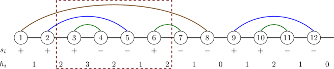
Figure 1: Illustrating the planar pairings. A set of $N=12$ sites, coupled by a planar pairing. Each site gets a spin value, $s_{i}=+1$ or $-1$. The height function, $h_{i}$ is shown in the bottom row. A block is marked, containing sites 3 to 6.

Let us assume that the nodes are indexed counterclockwise. We can now define for each node $i$ a value $s_{i}$ to be either $+1$ or $-1$ depending on whether it is the source or the sink of a bond, as shown in Fig. 1. Of course, the sum of all the $s_{i}$ around the full system should be zero: $\sum_{k=1}^{N}s_{k}=0$. The $s_{i}$ can be considered as slopes of a height function,

$$h_{i}\equiv\sum_{k=1}^{i}s_{k}.$$ (5)

Of course, this definition is not translation invariant, since we start counting at node 1. In order to avoid that, let $h_{0}$ denote the absolute minimum of this height function. Then, we can define the absolute height function, $H_{i}\equiv h_{i}-h_{0}$. Its meaning is the following: it denotes the number of bonds passing above the link in the circle joining nodes $i$ and $i+1$. By construction, this absolute height function has, at least, one zero.

II.2 Dyck Language and Catalan Numbers

There is a close analogy between planar pairings and the Dyck language Stanley.99 . A Dyck word is a string of symbols from the alphabet $\{+,-\}$ such that the number of $+$ counted from the left is always greater or equal to the number of $-$. Equivalently, they are the set of properly balanced parenthesis. This means that their height function $h_{i}$, as defined in Eq. (5), is positive for all $i$. The difference between our planar pairings and the Dyck language resides entirely in the periodic boundary conditions. If, in our circular planar structures, we break at the absolute minimum of the height function, the analogy with Dyck words becomes complete.

How many different planar states are there for a system of fixed size $N=2M$? Let us denote this value by $P_{M}$. Disregarding the ordering of the sites in each bond, which merely contributes a general $2^{M}$ factor, we can provide a recursive relation. Site 1 must be linked to an even site, $2k$. Then it creates two regions, one of size $2k-2$ and the other $2M-2k$. Thus, we get

$$P_{M}=\sum_{k=1}^{M}P_{k-1}P_{M-k}$$ (6)

along with $P_{2}=1$, which is known in the literature as Segner’s recurrence Stanley.99 , which gives rise to the Catalan numbers:

$$P_{M}={1\over M+1}{2M\choose M}$$ (7)

II.3 Entanglement of Planar States

Given a planar state of the form (4), we can easily compute the entanglement entropy of any block $B$: using 2 as the base for the logarithms, it coincides with the number of bonds which must be cut in order to separate it from the rest of the system Refael.04 ; Laflorencie.05 ; Ramirez.14 .

$$S(B)\equiv\sum_{p}[p_{1}\in B\;\oplus\;p_{2}\in B]$$ (8)

where $\oplus$ stands for the exclusive or (xor) symbol, which means that either $p_{1}\in B$ or $p_{2}\in B$, but not both. We can prove the following theorem which relates the height function and entanglement. Let $[i..j]$ denote the block $\{i,\cdots,j\}$. Then,

$$S(B_{[i..j]})=H_{i-1}+H_{j}-2\min_{k\in\{i-1\cdots j\}}H_{k}.$$ (9)

The meaning of that equation is the following. $H_{i-1}$ represents the bonds that enter the block from its left end, and $H_{j}$ the bonds which exit from its right. For an example, see Fig. 1. The block marked with the dashed box is $B_{[3..6]}$. The number of bonds entering from the left is $H_{2}=2$, and the number of bonds leaving from the right is $H_{6}=2$. But not all those bonds contribute to the entropy. Some of them just fly over the block, and we can separate the block without touching them. Let $h_{F}$ be the number of those flying bonds, in our example $h_{F}=1$, the bond from site 1 to site 8. The links entering from the left, $H_{i-1}$ are either overflying ($h_{F}$) or not ($h_{L}$): $H_{i-1}=h_{F}+h_{L}$. Similarly, on the right we have $H_{j}=h_{F}+h_{R}$, and the block entropy is given by $h_{L}+h_{R}$. We will proceed to prove that $h_{F}$ is given by the minimum of the height function inside the block. Since the bonds which contribute to the entropy, $h_{L}$ and $h_{R}$, do not fly over the block, they must either end inside it ($h_{L}$) or start inside it $h_{R}$. Since the bonds can not cut, the $h_{L}$ bonds from the left must have ended before any of the $h_{R}$ start. At that very moment, only the flying bonds will remain. In Fig. 1, this moment takes place between sites 5 and 6, $h_{L}=1$, $h_{R}=1$ and the block entropy is $S=2$. Thus, the minimum value of the height function is, exactly, $h_{F}$. We have $H_{i-1}+H_{j}-2h_{F}=h_{L}+h_{R}=S$, as required.

Notice that we can rewrite expression (9) as $S(B_{[i..j]})=(H_{i-1}-H_{min})+(H_{j}-H_{min})$, thus showing a connection between the block entropy and the average variation of the height within the block, i.e. the roughness of the interface. The main difference is that the entanglement entropy gives special relevance to the boundaries.

III Correlated random spin chains

The statistical properties of the ground states of Hamiltonians of the form (1) when the couplings $\{J_{i}\}$ are picked randomly and uncorrelated have been determined in a series of papers Dasgupta.80 ; Fisher.95 ; Refael.04 ; Laflorencie.05 ; Hoyos.07 ; Fagotti.11 ; Ramirez.14 . The SDRG procedure converges to the so-called infinite randomness fixed point (IRFP). Along the RG, the variance of the effective couplings grow, and their correlation length decreases. It has been shown that the average entanglement entropy of a block of size $\ell$ follows the expression Fagotti.11 ; Ramirez.14 :

$$S(\ell)\approx\log(2)\;{c\over 3}\;\log\left({N\over\pi}Y\left({\pi\ell\over N}\right)\right)+c^{\prime},$$ (10)

where $Y(x)$ is a scaling function and $c$ is the central charge of the associated CFT, i.e., the one which corresponds to the homogeneous (conformal) case, with all the $J_{i}$ equal. In our case, $c=1$. Surprisingly, expression (10) is very similar to the conformal expression Vidal.03 :

$$S_{CFT}(\ell)\approx{c\over 3}\;\log\left({N\over\pi}\sin\left({\pi\ell\over N}\right)\right)+c^{\prime}.$$ (11)

The scaling function $Y(x)$ is, in fact, rather similar to $\sin(x)$ Fagotti.11 ; Ramirez.14 .

Another relevant observable which helps characterize the IRFP is the bond-length probability, i.e., given a singlet bond $(i,j)$, determine the probability distribution for its length $l=|i-j|$, $P_{B}(l)$. This value is directly related to the two-point correlation function Fisher.95 . In the uncorrelated case, it is known to behave, for $l\ll N$, as a power-law: $P_{B}(l)\approx l^{-\eta}$, where $\eta=2$ Fisher.95 .

III.1 Correlated couplings

Our aim is to characterize the ground states of Hamiltonian (1) when the couplings $J_{i}$ are random, but present non-trivial correlations. If these correlations are short ranged, they will be washed away by the renormalization procedure, and return to the IRFP. Thus, we will consider the case of long-range correlations.

Let us establish a procedure to obtain samples from sets of log-couplings $\{t_{i}\}$ which present long-range correlations, by employing a suitable Fourier expansion:

$$t_{j}=\sum_{k}A_{k}\sin(jk+\phi_{k})$$ (12)

where $k$ are a set of allowed momenta, $k_{n}=2\pi n/N$, with $n\in\{1,\cdots,2N\}$. We do not include moment zero, since it would amount to a global constant which would be irrelevant for the SDRG. The values $A_{k}$ and $\phi_{k}$ are chosen as independent random variables. The phase $\phi_{k}$ is taken to be uniformly distributed in $[0,2\pi)$ and

$$A_{k}=k^{-\gamma}u_{k},$$ (13)

where the $u_{k}$ are independent gaussian variates with zero average and variance one, and $\gamma$ is a fixed spectral exponent.

If $\gamma=0$, all momenta in expression (12) get the same weight, and we obtain again an uncorrelated set of $t_{i}$. As we increase $\gamma$, the larger momenta get less and less weight, and we are left with only the lowest momenta. This implies that the set of $t_{i}$ have stronger correlations. Fig. 2 (A) shows typical samples for increasing values of $\gamma$.

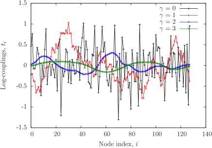
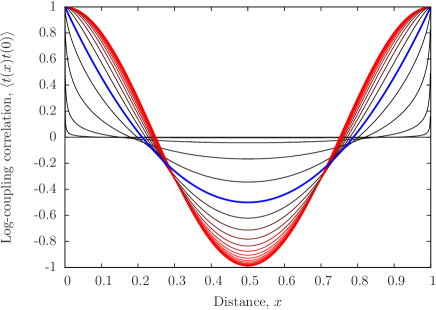
Figure 2: (A) samples of $\{t_{i}\}$ for $N=128$ and increasing values of $\gamma$. (B) real-space correlation function for several values of $\gamma$ from zero (black) to infinity (red), obtained analytically for $N=1000$, from expression (14). The value $\gamma=1$ appears remarked in blue.

The ensemble of log-couplings presents zero correlations in momentum space, but strong correlations in real space for increasing $\gamma$. The correlation function is translation invariant by construction, and given by

$$\left<t(x)t(0)\right>\propto\sum_{k\geq 2\pi/N}{1\over k^{2\gamma}}\cos(kx)$$ (14)

For $N=1000$, Fig. 2 (B) shows the correlation as a function of the distance, normalized to have a maximal value of one. For $\gamma=0$, the correlation is identically zero for all $x>0$. For $\gamma\to\infty$ it approaches a cosine function. The value $\gamma=1$, which will have special relevance in the rest of the text, appears marked. We should remark that, although Eq. (14) makes perfect sense for all finite values of $N$, the expression diverges in the thermodynamic limit for $\gamma\leq 1/2$.

Fig. 3 shows some sample planar pairings for different values of $\gamma$, in the range from $\gamma=0$ (no correlations) to $\gamma=3$ (large correlations), along with their corresponding height diagrams.

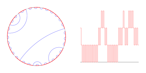
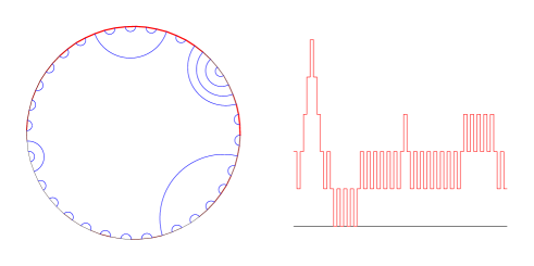
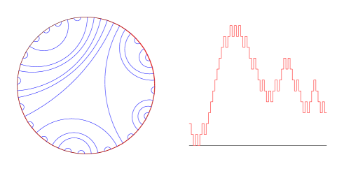
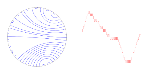
Figure 3: Bond diagrams for different samples with $N=64$ and $\gamma$ running (downwards) from $\gamma=0$ to $\gamma=3$. To their right, the corresponding height profiles.

III.2 Entanglement, Roughness and Bond-Lengths

The average entanglement entropy as a function of the block size $\ell$, for a fixed value of $N=1000$, $10^{5}$ realizations and several values of $\gamma$ is shown in Fig. 4 (A). The upper part of the panel is devoted to $\gamma\geq 1$, while the lower one shows more detail for $\gamma\leq 1$. Notice that, for $\gamma\leq 1$, the function $S(\ell)$ is nearly independent of $\gamma$. We propose a finite-size fit of the form:

$$S(\ell)\approx A\left(N\,Y(\pi\ell/N)\right)^{\chi},$$ (15)

where the scaling function $Y(x)$ is determined via a Fourier series expansion in the same line as Fagotti.11 ; Ramirez.14 :

$$Y(x)=\sin(x)+\sum_{n=1}^{\infty}\alpha_{n}\sin((2n+1)x).$$ (16)

The best fit values of $\alpha_{n}$ are small and nearly independent of the spectral exponent $\gamma$. We have found $\alpha_{1}\approx 0.05$ and $\alpha_{2}\approx 0.005$, both slowly decaying as $\gamma$ increases. The inset of the top panel of Fig. 4 shows these scaling functions for different values of $\gamma$.

The values of the exponent $\chi$ present more relevance. Fig 4 (B) show these exponents, found by three different strategies: (i) Finite-size, using a full fit to expression (15) for $N=1000$, (ii) Local exponent, fitting the entropy for small blocks to a form $S(\ell)\approx\ell^{\chi}$ also for $N=1000$, (iii) Global exponent, fitting $S(N/2)$ to a form $N^{\chi}$ for different values of $N$, up to $N=2000$. The three expressions differ slightly for larger $\gamma$, although they keep a general trend: for $\gamma\leq 1$, $\chi$ is very close to zero, while for $\gamma\to\infty$ we see $\chi\to 1$. This signals a volumetric growth of the entropy $S\sim\ell$. The discrepancies between the values of $\chi$ measured by the different strategies, as seen in Fig. 4 (B), may be of numerical origin.

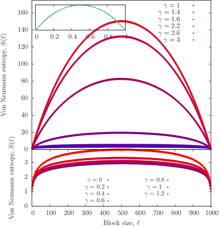
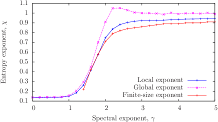
Figure 4: (A) Average block von Neumann entropy as a function of the block size for different values of $\gamma$, with $N=1000$. Top panel: $\gamma\geq 1$. Bottom panel: $\gamma\leq 1$. Inset: scaling function, $Y(x)$ as in Eq. (16). (B) Fitting exponent $\chi$ as a function of $\gamma$ for the three strategies discussed in the text.

Interestingly, for $\gamma\leq 1$, the $S(\ell)$ curves are nearly identical, and the best finite-size fit to the whole function is not given by the power-law expression (15), but expression (10), i.e. a logarithmic behavior. Even for $\gamma\approx 1$, the best fit is logarithmic, but with a slightly larger prefactor. It is difficult to determine whether there is a smooth crossover between $\gamma=0$ and $\gamma\to\infty$ or a sharp transition at $\gamma\approx 1$, below which the entropy grows logarithmically, i.e.: if the IRFP extends to the region $\gamma\leq 1$.

Another interesting observable is provided by the study of the height function which characterizes the state, given by eq. (5). As we will show, the profiles are fractals, of similar nature to the ones appearing in the study of rough interfaces Family.85 ; Barabasi.95 . Let us define the roughness, or width $W$, of the interface for a given length scale $\ell$ as the average deviation of the heights in windows of that size. Then, the Family-Vicsek Ansatz assumes that $W\sim\ell^{\alpha}$. Fig. 5 (A) shows the roughness as a function of the window size $\ell$, taking $10^{5}$ realizations for each value of $\gamma$. The top frame shows a log-log plot, while in the bottom one only the $x$-axis is logarithmic. The difference is notorious: for $\gamma>1$, the roughness follows a clear power law, with exponent $\alpha$ which grows up to one (shown as a straight line). For $\gamma\leq 1$, instead, the behavior is better fit by a logarithmic function $W(\ell)\sim\log(\ell)$. This provides further support to the conjecture that the behavior for $\gamma\leq 1$ corresponds to the IRFP.

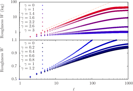
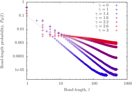
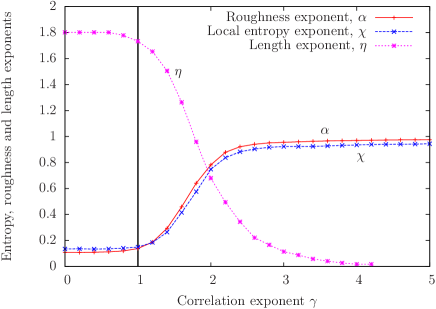
Figure 5: (A) Roughness of blocks, $W(\ell)$, of different sizes, for $N=1000$ and different values of $\gamma$. The top frame is in log-log, while the bottom one only the $x$-axis is logarithmic. This way we can show that for $\gamma\leq 1$, the best fit is for a logarithmic growth of the roughness. (B) Bond-length distribution, also for $N=1000$, using the minimal length. Notice that the lines are parallel for $\gamma=0$ and $\gamma=1$, but shifted. They have the same scaling exponent, but different prefactor. (C): fitting exponents for the entropy ($\chi$), roughness ($\alpha$) and bond-length ($\eta$) as a function of $\gamma$. Below the $\gamma=1$ line, it can be argued that the roughness and the entropy do not behave like a power law, but instead they show logarithmic behavior.

Panel (B) of Fig. 5 depicts the probability distribution for the bond-length. A power-law is established, i.e., $P_{B}(l)\sim l^{-\eta}$, and $\eta$ is shown to depend on $\gamma$. For $\gamma\leq 1$, the curves appear to be parallel, i.e., show the same exponent, and only differing in their prefactor foot:renormalized .

Fig. 5 (C) shows the values of the three exponents, entropy ($\chi$), roughness ($\alpha$) and bond-length distribution ($\eta$) as a function of the correlation parameter $\gamma$. Notice that $\chi$ is very similar to $\alpha$, as suggested by relation (9) which links the block entropy to the height fluctuations. Both exponents grow with $\gamma$, starting near zero for uncorrelated spin chains and saturating at a value close to 1. The bond-length exponent $\eta$ behaves in the opposite way, starting at $\eta=2$ for uncorrelated spin chains and decreasing towards zero. The region for $\gamma\leq 1$ is peculiar: while the bond-length $\eta$ exponent is still $2$, the other two exponents are very close to zero, since the true behavior is expected to be logarithmic.

The limit $\gamma\to\infty$ is also rather special. A look at the last panel of 3 shows that rainbow-like structures become more and more prominent. The limit in which only the lowest momentum modulation survives gives rise to a perfect rainbow state, which presents volumetric entanglement Vitagliano.10 ; Ramirez.15 , i.e., $S\sim\ell$. This explains the limit $\chi\to 1$ for the entropy exponent for large $\gamma$. Similarly, the height function becomes a nearly perfect wedge, which explains the $\alpha\to 1$ behavior. In that extreme, the bond-length distribution is completely flat, since all bond-lengths show up once for each realization, thus $\eta=0$.

IV RNA folding and Spin Chains

As it was briefly discussed in the introduction, planar pairings also appear naturally in the study of the secondary structure of folded RNA strands Tinoco.99 . The model developed by Wiese and coworkers Wiese.06 ; Wiese.08 works in the following way: (1) a pair of sites with different parity are chosen randomly and paired; (2) further pairs are chosen in the same way, always under the constraint that no previous bonds can be crossed. In their seminal work Wiese.08 , the authors studied the roughness of the equivalent height function and the bond-length distribution, showing that they both follow a power-law behavior, $W\sim\ell^{\alpha}$ and $P_{B}(l)\sim l^{-\eta}$. Then they proved that $\alpha+\eta=2$. If we assume the scaling equivalence of the roughness and the entropy, this result is also fulfilled in uncorrelated random spin chains, where we have $\alpha=0$ (because of the logarithmic behavior of the entropy) and $\eta=2$ Refael.04 ; Ramirez.14 . On the other hand, this relation does not hold for correlated spin chains.

We may ask what is the range of validity of the relation $\chi+\eta=2$ (or $\alpha+\eta=2$). Extending the results of Hoyos.07 ; Ramirez.14 we can provide a proof of that statement in the case of uncorrelated bonds. Indeed, let us consider a block of size $\ell$ and let us number the sites from $1$ to $\ell$. The bond at site $i$ will be cut by the block if it goes left and its length is larger or equal than $i$, or if it goes right and its length is larger than $\ell-i$. So, we have an estimate for the average entropy:

$$S(\ell)\approx\sum_{i=1}^{\ell}{1\over 2}\left(P_{B}(l\geq i)+P_{B}(l>\ell-i)\right)=\sum_{i=1}^{\ell}P_{B}(l\geq i)$$ (17)

This equation implies a double integration. If $P_{B}(l)\sim l^{-\eta}$, it leads to $S(\ell)\sim l^{-\eta+2}$, as we desired. As it follows from Fig. 5 (C), this is not true for the planar state ensembles generated with correlated couplings. In fact, in the rainbow limit, we have $\chi+\eta\to 1$, which suggests a strong correlation between the bonds.

IV.1 The inverse problem

How strong is the connection between the RNA folding and disordered spin chains? Can we obtain an ensemble of couplings $\{J_{i}\}$ such that the ground states of Hamiltonian (1) correspond to the planar states obtained in RNA folding? This question leads us to the study of the more general inverse SDRG problem.

If we regard the SDRG as a mapping between sets of couplings and planar pairings, we might be able to reverse the algorithm, and obtain the set of couplings which give rise to a certain planar pairing. In other terms, a parent 1D Hamiltonian for a given planar state. In this section we will show that (1) every planar state has a (non-unique) parent 1D Hamiltonian and (2) an explicit algorithm to obtain the optimal set of couplings, in a sense to be determined later.

The aim is to obtain the logarithmic couplings, $\{t_{i}\}$, given the set of bonds, $\{{\bf p}_{i}\}$. Our proposed algorithm works as follows (see Fig. 6 for an illustration):

• Sort the bonds in order of increasing length.

• Consider the bonds of length one, fix their internal log-couplings to $0$. In the first row of Fig. 6, we put a zero under links $3-4$ and $10-11$.

• Flank these zeroes with log-couplings of value $1$ at both sides. See the second row of Fig. 6, where the arrows in the new values point to the zero which they flank.

• Now consider the bonds of length three. Find the effective log-coupling which would appear as their renormalization value (which must be 2). Flank them with log-couplings of value $2+1=3$ at both sides, as in the third row of Fig. 6.

• Consider the rest of the bonds in order of increasing lengths. For each of them, find their renormalization value and flank them with log-couplings of value one unit higher.

• Log-couplings may never decrease along the procedure. If two values collide, take the larger.

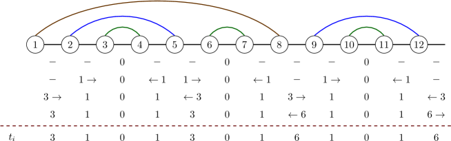
Figure 6: Illustration of the inverse algorithm to obtain the optimal log-couplings which give rise, via the SDRG, to a given planar bond structure. Each row corresponds to one of the steps of the algorithm. The log-couplings which have not been assigned yet appear as a “$-$”. The arrows which appear close to a new value point to the bond which has created (or modified) that value.

This procedure yields couplings which, by construction, always give rise to the desired bond structure. Moreover, because the value of each bond is computed using the SDRG itself, we ensure a certain optimality condition: among the sets of couplings yielding the desired state, our choice will always require the minimal span of coupling values. For example, this Hamiltonian will yield the largest possible gap.

Fig. 7 (A) shows the couplings which give rise to a give instance of the RNA folding problem with $N=100$. We have run $10^{5}$ simulations of the RNA folding algorithm and obtained the optimal couplings for different system sizes up to $N=1000$. Fig. 7 (B) shows the (translation invariant) correlation function for the log-couplings in the $N=50$, $100$ and $200$ cases. The values present long range correlations, but not a clear power-law behavior. Moreover, the couplings field $\{t_{i}\}$ is not gaussian. In the inset of Fig. 7 (B) we show the histogram, in logarithmic scale, for $t_{i}$. The marginal probability distribution is not gaussian. Instead, it is a power-law, with an empirical exponent close to $-4/3$.

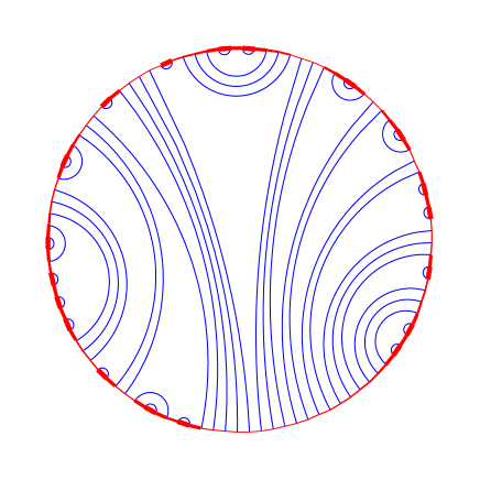
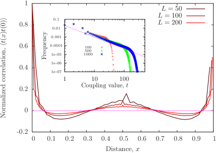
Figure 7: (A) The optimal couplings which give rise to a given planar pairing obtained from the RNA folding algorithm with $N=100$. (B) The correlation function for the log-couplings at different points for $N=50$, $100$ and $200$, using $10^{6}$ realizations. Inset: histogram for the log-coupling values for $N=100$, $500$ and $1000$, also with $10^{6}$ realizations. Notice the power-law inertial range, with an exponent close to $-4/3$ (straight line).

V Generic planar states

Since we have determined that all planar states have a 1D parent Hamiltonian, we may still ask how dense are planar states within the Hilbert space. In other terms, how generic they are. We can define an ensemble of planar states for $N$ sites under the condition that all possible planar pairings have the same probability. In order to sample that ensemble, we just apply a correction to the RNA folding sampling strategy. In the RNA folding algorithm, the pair of sites $(i,j)$ which will constitute the next bond is chosen with equal probabilities among those which do not cut any previous bond. But, following that procedure, not all planar pairings are sampled with the same probability. This can be corrected if the probabilities for each pair $(i,j)$ are not equal, but proportional to the number of planar pairings which are consistent with the presence of that bond.

Let us consider a certain empty patch of length $n$ in a planar pairing which is under construction, i.e., a set of contiguous spins which have not been paired yet. As we know, there are $P_{n}$ possible ways to create a planar pairing on that empty patch. The spin with index 1 must be paired with some spin inside the patch, let us refer to its index as $k$. Then, after bond $(1,k)$ is established, the number of different possible planar pairings will be $P_{k-2}P_{n-k}$. Thus the probability with which bond $(1,k)$ should be taken is just $P_{k-2}P_{n-k}/P_{n}$, which is known to be less than one by construction, as we see in Eq. (6). Repeating this procedure, we can sample the planar pairing ensemble with equal probabilities.

We have found numerically the average block entropy as a function of the block size $\ell$ for this ensemble of states, and found that it grows as $S(\ell)\sim\ell^{\chi}$, with $\chi\approx 0.54$. The precise value is not very relevant, but it allows us to conclude that planar states are highly non-generic quantum states, because for generic states we should obtain $S(\ell)\sim\ell$, i.e., a volumetric growth of the entropy.

VI Conclusions and Further Work

In this article we have applied the SDRG to study the ground state properties of a strongly disordered random spin chain with long-range correlations between its couplings. The states can be described as valence bond states with planar bond structures, and they can have arbitrarily large entanglement entropy. Concretely, we have chosen the couplings such that their logarithm is expressed as a Fourier series with random coefficients, falling as a power-law of the momentum $k^{-\gamma}$. For $\gamma\leq 1$ the behavior is very similar to the infinite randomness fixed point (IRFP) found for uncorrelated coupling constants. Nonetheless, for $\gamma>1$, the block entropy behaves as a power-law of the block size, $S\sim\ell^{\chi}$, with $\chi$ a function of the exponent $\gamma$ which seems to interpolate smoothly between $\chi=0$ and $\chi=1$ as $\gamma\to\infty$. The bond length probability, which is related to the correlator, is also characterized by a power-law, $P_{B}(l)\sim l^{-\eta}$, with $\eta=2$ for $\gamma\leq 1$ and falling to $\eta\sim 0$ for $\gamma\to\infty$. This extreme, $\gamma\to\infty$, corresponds to the case where only the lowest momentum $k=2\pi/N$ contributes to the correlation between the couplings, and the state becomes a rainbow state. As we have shown, the planar states can be mapped to a 1D interface, whose roughness behaves approximately like the entanglement entropy, as it is suggested by expression (9). Remarkably, the system described constitutes a family of local 1D Hamiltonians whose ground states violate the area law to any desired degree.

We have also considered the inverse renormalization problem: given a (planar) valence bond state, to obtain its (1D) parent Hamiltonian. In this way we were able to study the ensemble of random spin chains whose ground states would correspond to the planar structures which show up in other physical situations, such as the RNA folding problem. These engineered random spin chains present a behavior of the entanglement entropy and the correlators which do not correspond to any value of $\gamma$. This suggests that the phase diagram of random spin chains with large correlations between the couplings is richer than expected.

Inhomogeneous spin chains can be mapped, in some cases, to models which represent the motion of fermionic matter on a curved spacetime Boada.11 , where the metric is given by the coupling constants. Thus, our study shows that the statistical properties of the metric show up as statistical properties of the entanglement of the vacuum, i.e., the ground state of the corresponding Hamiltonian. Moreover, we can also find, using the inverse renormalization algorithm, the optimal spatial geometry which gives rise to a certain vacuum entanglement. These results may shed light on the relation between entanglement and space-time Maldacena.13 .

- (1) G Refael, JE Moore, “Entanglement entropy of random quantum critical points in one dimension”, Phys. Rev. Lett. 93 260602 (2004).
- (2) N Laflorencie, “Scaling of entanglement entropy in the random singlet phase”, Phys. Rev. B 72, 140408(R) (2005).
- (3) A Hoyos, AP Vieira, N Laflorencie, E Miranda, “Correlation amplitude and entanglement entropy in random spin chains”, Phys. Rev. B 76, 174425 (2007).
- (4) G Ramírez, J Rodríguez-Laguna, G Sierra, “Entanglement in low-energy states of the random-hopping model”, JSTAT P07003 (2014).
- (5) PW Anderson, “Absence of diffusion in certain random lattices”, Phys. Rev. 109 1492 (1958)
- (6) G Vidal, JI Latorre, E Rico, A Kitaev, “Entanglement in quantum critical phenomena”, Phys. Rev. Lett. 90 227902 (2003).
- (7) J Eisert, M Cramer, MB Plenio, “Colloquium: Area laws for the entanglement entropy”, Rev. Mod. Phys. 82, 277 (2010).
- (8) P Calabrese, J Cardy, J. Phys. A.: Math. Theor 42, 504010 (2009).
- (9) C Dasgupta, S-K Ma, “Low-temperature properties of the random Heisenberg antiferromanetic chain”, Phys. Rev. B 22 1305 (1980).
- (10) DS Fisher, “Critical behavior of random transverse-field Ising spin chains”, Phys. Rev. B 51 6411 (1995).
- (11) G Vitagliano, A Riera, JI Latorre, “Volume-law scaling for the entanglement entropy in spin-1/2 chains”, New J. of Phys. 12, 113049 (2010).
- (12) G Ramírez, J Rodríguez-Laguna, G Sierra, “From conformal to volume-law for the entanglement entropy in exponentially deformed critical spin 1/2 chains”, JSTAT P10004 (2014).
- (13) G Ramírez, J Rodríguez-Laguna, G Sierra, “Entanglement over the rainbow”, JSTAT P06002 (2015).
- (14) I Tinoco, C Bustamante, “How RNA folds”, J. Molec. Biol. 293, 271 (1999).
- (15) M Lässig, KJ Wiese, “Freezing of random RNA”, Phys. Rev. Lett. 96, 228101 (2006).
- (16) F David, C Hagendorf, KJ Wiese, “A growth model for RNA secondary structures”, JSTAT P04008 (2008).
- (17) RP Stanley, “Enumerative combinatorics”, Vol. 2, Cambridge Univ. Press (1999).
- (18) AL Barabasi, HE Stanley, “Fractal concepts in surface growth”, Cambridge Univ. Press (1995).
- (19) F Family, T Vicsek, “Scaling of the active zone in the Eden process on percolation networks and the ballistic deposition model”, J. Phys. A: Math. & Gen. 18, 75 (1985).
- (20) M Fagotti, P Calabrese, JE Moore, Phys. Rev. B 83, 045110 (2011).
- (21) P Di Francesco, O Golinelli, E Guittier, “Folding, meanders and arches”, in “Low dimensional applications of quantum field theory”, Ed. L Baulieu et al., Plenum Press (1997).
- (22) O Boada, A Celi, JI Latorre, M Lewenstein, “Dirac equation for cold atoms in artificial curved spacetimes”, New J. Phys. 13 035002 (2011).
- (23) J Maldacena, L Susskind, “Cool horizons for entangled black holes”, Fortschr. Phys. 61 781 (2013).
- (24) Instead of using the minimal length of the bond, we can also employ their renormalized length, i.e., the number of links which were decimated in its formation during the SDRG procedure. As opposed to the minimal length, the renormalized length can be larger than . This alternative definition does not affect the computation of entropies, but it changes the heights and the bond-lengths. But the universal features described in this chapter were not changed, and thus we do not show specific results.