Optimizing spinning time-domain gravitational waveforms for Advanced LIGO data analysis      

Abstract

The Spinning Effective One Body-Numerical Relativity (SEOBNR) series of gravitational wave approximants are among the best available for Advanced LIGO data analysis. Unfortunately, SEOBNR codes as they currently exist within LALSuite are generally too slow to be directly useful for standard Markov-Chain Monte Carlo-based parameter estimation (PE). Reduced-Order Models (ROMs) of SEOBNR have been developed for this purpose, but there is no known way to make ROMs of the full eight-dimensional intrinsic parameter space more efficient for PE than the SEOBNR codes directly. So as a proof of principle, we have sped up the original LALSuite SEOBNRv2 approximant code, which models waveforms from aligned-spin systems, by nearly 300x. Our optimized code shortens the timescale for conducting PE with this approximant to months, assuming a purely serial analysis, so that even modest parallelization combined with our optimized code will make running the full PE pipeline with SEOBNR codes directly a realistic possibility. A number of our SEOBNRv2 optimizations have already been applied to SEOBNRv3, a new approximant capable of modeling sources with all eight (precessing) intrinsic degrees of freedom. We anticipate that once all of our optimizations have been applied to SEOBNRv3, a similar speed-up may be achieved.

1 Introduction

The Advanced Laser Interferometer Gravitational-wave Observatory [1] (LIGO) and the French-Italian gravitational wave detector, VIRGO, [2] are the most sensitive gravitational-wave interferometers that have ever been constructed. Although Initial/Enhanced LIGO/VIRGO did not detect gravitational waves [3], Advanced LIGO [1] achieved unprecedented sensitivities during its first observing run and detected gravitational waves for the first time [4].

Spins and masses of compact objects can be inferred from detected gravitational waves through a Bayesian model approximation using Markov chain Monte Carlo (MCMC) methods implemented in lalinference [5]. Ideally, the theoretical waveforms required for these methods will be based entirely on full solutions to Einstein’s equations (numerical relativity). On the surface this seems promising, as numerical relativity work can reliably solve the full set of Einstein’s equations for all compact binary systems of interest for Advanced LIGO, and can even generate gravitational waves for long inspirals. For example, state-of-the-art numerical relativity simulations have successfully generated a 350-cycle black-hole binary gravitational waveform that spans the entire LIGO band for systems with total mass over $45.5M_{\odot}$ [6]. Unfortunately, generation of this single waveform spanned months on a high-performance computing resource, and traditional MCMC parameter estimation (PE) across the full space of possible binary parameters will require $\sim 10^{8}$ waveforms to be generated sequentially. Therefore, full parameter estimation for a single observed wave using current numerical relativity techniques and resources could require $\sim$5 million years, or roughly 7 orders of magnitude too long to be useful for LSC work.

There are a number of strategies for overcoming this enormous computational challenge, generally relying on perturbative and/or phenomenological solutions to Einstein’s equations. Since numerical relativity directly solves the full set of Einstein’s equations, it can be argued that the most accurate approximants will incorporate numerical relativity solutions. However, all approximants possess their own set of systematic errors.

As an example, consider the “Phenom” family of phenomenological gravitational waveform models [7, 8, 9, 10]. Recent “Phenom” models use the state-of-the-art, purely perturbative SEOBv2 (Spinning Effective One-Body, version 2) model for the inspiral part of the waveform (i.e., an uncalibrated version of the [11] model), and for merger and ringdown, attach a phenomenological waveform calibrated to $\sim 20$ numerical relativity waveforms [9].

“Phenom” models have the great advantage of being able to generate theoretical waveforms extremely fast and in the frequency domain directly, which simplifies most data analyses. As a result, they are one of the bedrocks of LSC parameter estimation. That being said, both “Phenom” and SEOBNR models possess unique systematic uncertainties that are magnified by the fact that few numerical relativity waveforms exist that are sufficiently long to fully uncover systematic errors in approximate models across the full parameter space. Therefore, there is a strong need for fully independent gravitational wave approximants with different systematic uncertainties that are capable of spanning the widest parameter space possible. Perhaps more importantly, given the significantly different approaches used to model the signal using each technique, there is good reason to hope that their systematic uncertainties will be independent of one another, so they can be used to better understand the overall systematic uncertainties resulting from waveform modeling errors.

The SEOBNR series of waveform models [12, 13, 14, 15, 16, 17, 18, 19, 20, 11, 21] fill this gap extremely well. Although the calculation of the inspiral by SEOBNRv2 and the most recent version of Phenom are not entirely independent [9], the merger and ringdown are entirely independent. The SEOBNR approximant, [11], which is currently on its second version (SEOBNRv2), contains much of the relevant physics, including spin-orbit effects up to order 3.5PN [22], and the ability to model varying mass ratios and individual spin magnitudes for each compact object; it lacks only the ability to model spins that are not aligned with the orbital angular momentum, and therefore precess over time. This feature has only now been added to the third version (SEOBNRv3).

Like “Phenom” models, SEOBNR models have been shown to produce waveforms that agree well with some of the latest numerical relativity black-hole binary waveform calculations. Though SEOBNR is truly a state-of-the-art approximant, like any approximant it possesses systematic uncertainties, again magnified by the fact that there are so few numerical relativity waveforms against which it could be calibrated, particularly for systems with precessing spins. Despite their very strong pedigree, SEOBNR waveform models—as they have been officially implemented in LALSuite [23] (the LSC’s open-source data analysis software repository)—are extremely slow, requiring roughly six minutes to generate a single binary neutron star waveform that spans the entire Advanced LIGO band, given a start frequency of 10 Hz and a waveform sample rate set to 16,384 Hz, which is the LALSuite default output frequency. SEOBNRv2-based parameter estimation using standard MCMC, which requires the generation of $\sim 10^{7}$ sequential waveforms [25], would therefore take $\sim$100 years to complete using current computer hardware. The time required increases to a millennium for the $\sim 10^{8}$ sequential waveforms necessary for parameter estimation across the full eight dimensions of intrinsic black-hole binary parameter space [5]. As we will show, since such a large number of sequential waveforms generations are required, our optimizations are absolutely essential to making possible a full eight-dimensional pipeline using SEOBNR codes directly.

As evidence of the importance of the SEOBNR series, an “industry” has been built up within the gravitational-wave data-analysis community around constructing Reduced Order Models (ROMs) of SEOBNR waveforms (e.g., [26, 24, 27]). ROMs are built from a large sample of computed waveforms from SEOBNR models, and take advantage of the fact that a small perturbation in initial binary parameters will result in a small perturbation in the resulting waveform; reduced bases and interpolated parameter dependent coefficients are integral building blocks in the construction of ROMs. In short, ROMs generate waveforms between sampled points using what amounts to multidimensional interpolations, though this may introduce small interpolation errors.

ROMs of SEOBNR models have been hugely successful so far, resulting in speed-up factors of $\sim 10^{4}$ over the original SEOBNR codes within LALSuite [24, 27]. Unfortunately, by their nature ROMs would need to be regenerated if any recalibration to the underlying model is made, which can be an expensive process. Further, SEOBNRv2 ROMs have only been generated for up to four of the eight dimensions of intrinsic black-hole binary waveform parameter space, for which only $\sim 10^{7}$ sequential waveforms might need to be generated. To make matters worse, due to technical challenges there is currently no method available for efficiently producing ROMs to cover the full eight-dimensional precessing-spin parameter space. Unless a breakthrough is made and ROMs can be extended to all eight dimensions, their usefulness for generic parameter estimation will be severely jeopardized (see e.g., [28]). At this point in time, the only way to generate SEOBNR models over the full, eight-dimensional parameter space is to use the (slow, not-fully-optimized) SEOBNRv3 code within LALSuite itself.

So, in anticipation of a breakthrough leading to SEOBNR ROMs over the full eight-dimensional parameter space, and in preparation for the release of the eight-dimensional SEOBNR approximant (SEOBNRv3, which was undergoing code review while this paper was being written), in this paper we describe our efforts in improving the performance of the four-dimensional, second version of SEOBNR (SEOBNRv2) used in LALSuite by more than two orders of magnitude in terms of execution time.

We stress that each optimization to SEOBNRv2 presented in this paper has its analogue in SEOBNRv3, and some have already been included in the SEOBNRv3 currently under development within LALSuite. Our fully optimized SEOBNRv2 now exists within LALSuite under the moniker SEOBNRv2_opt.

After all of our optimizations, the overall speed-up factor of SEOBNRv2, given by the waveform cycle-weighted average,

$$\mathcal{S}=\frac{\sum_{i}\mathcal{S}_{i}N_{{\rm wc},i}}{\sum_{i}N_{{\rm wc},i}}\,,$$ (1)

was found to be $\sim 300$, where $\mathcal{S}_{i}$ is the speed-up factor in generating the $i$’th waveform and $N_{{\rm wc},i}$ is the number of wavecycles in the $i$’th waveform.

Thus we have reduced the timescale for full PE using SEOBNRv2 directly from 10–100 years to between weeks and months, which now makes it possible to perform PE using SEOBNRv2 codes directly. Core to our optimization philosophy was ensuring that SEOBNRv2_opt agrees with the original SEOBNRv2 code to the maximum degree possible (numerical roundoff error). To give an idea of this very harsh standard we set for ourselves, of all 1,600 waveforms sampled in this paper (across a wide swath of parameter space that included all three compact binary systems of central interest to Advanced LIGO/VIRGO), the largest amplitude-weighted average phase difference (Eq. 3) was less than 0.008 rad (Table 3). Advanced LIGO is at best sensitive to phase differences of $\approx 0.17$ rad and amplitude differences of order $10\%$, [4] due to calibration uncertainties. This is orders of magnitude beyond the maximum amplitude and phase differences measured when comparing optimized versus unoptimized SEOBNRv2 codes, so we conclude that our optimized SEOBNRv2 code can be used as a drop-in replacement to the original code without any impact on PE.

2 Optimization Strategies

LALSuite’s second SEOBNR code, SEOBNRv2 [11], which models waveforms from aligned spin systems, is the focus of optimization efforts in this paper. Next, we review the general strategies for optimizing SEOBNRv2, as well as the optimizations themselves.

Due to the necessity to frequently recompile and rerun the executables during the optimization process, as well as the desire to isolate core SEOBNRv2 functionality from other approximants within LALSuite, we extracted the core functions required by the SEOBNRv2 approximant from LALSuite into an independent standalone code. This was achieved through iteratively including functions the compiler requested as necessary for compilation. Once completely extracted and debugged, the standalone code’s outputs were verified to be identical to that of the original lalsimulation software to within roundoff error.

2.1 Basic Overview of SEOBNRv2 Code

For the purposes of optimization, we divide SEOBNRv2 into three components:

1. ODE Solver: The “ODE Solver” reads in initial parameters, generates initial data, and solves the SEOBNRv2 Hamiltonian equations of motion [18, 11]. This part requires that several derivatives of the SEOBNRv2 Hamiltonian be evaluated $\gtrsim 100,000$ times for a typical inspiral calculation starting at 10 Hz. Note that double neutron star (DNS) waveforms are the most costly to generate; for sources with a sufficiently large number of wave cycles, the overall time to generate a given waveform scales is dominated by this step, and scales roughly linearly with the number of cycles (as shown in the right panel of Fig. 1).

2. Waveform Generation: The full SEOBNRv2 time-domain waveforms are generally Fourier transformed into frequency space, which requires that the waveform be evenly sampled in time. However, for efficiency an adaptive timestep Runge-Kutta-type solver is adopted to solve the SEOBNRv2 equations of motion, so the ODE solution must be interpolated in time to achieve the evenly time-sampled solution required for the Fourier transform. As the input to this portion of the code is the solution to the SEOBNRv2 equations of motion and the output is the evenly time-sampled wave strain $h_{+,\times}(t)$, we call this the “Waveform Generation” part of the code.

3. QNM Attachment: The SEOBNRv2 equations of motion will generate the full inspiral and merger portions of the waveform. In the “QNM Attachment” code, the quasi-normal mode (QNM) ringdown waveform is attached to the ODE solution. This component of the SEOBNRv2 code constituted an insignificant portion of the overall run time during the first $\sim$300x speed-up effort. After all the speed-ups were included, it contributed $\sim$20% of the overall run time, so this portion of the code may need to be a focus of future optimizations.

2.2 SEOBNRv2 Optimizations

We summarize the six highest-impact optimizations below, with timing benchmarks (italicized) and speedup factors (italicized, in parentheses) at each step of the optimization process, using the 16,277 wave cycle $1.4M_{\odot}+1.4M_{\odot}$ double neutron star binary merger scenario as our test for benchmarking (with a start frequency of 10 Hz). Double neutron star binaries were chosen to measure overall speed-up factors because they are the most costly to generate.

1. 370 s Original, un-optimized SEOBNRv2.

2. 197 s (1.9x) Change from the gcc [29] to the Intel compiler v15.0.1 [30]. The Intel Compiler Suite (Intel compiler) is well known to often generate far more optimized executables than the GNU Compiler Collection (gcc).

3. 133 s (2.8x) Hand-optimize SEOBNRv2 Hamiltonian algebraic expressions, removing all unnecessary calls to expensive transcendental functions, like exp() and log().

4. 23.1 s (16x) Replace all finite difference derivatives of the SEOBNRv2 Hamiltonian with exact expressions automatically generated by Mathematica [31].

   This replacement improves code performance in two ways. First, it reduces the large amount of roundoff-error-induced noise from finite differencing, enabling the adaptive-timestep ODE solver (Runge-Kutta fourth order) to achieve the desired accuracy in fewer steps. Second, evaluating derivatives exactly calls for significantly fewer arithmetic operations than calling the original Hamiltonian multiple times as required to compute a finite difference derivative.

5. 7.06 s (52x) Reduce number and cost of interpolations inside the Waveform Generation component of the code.

   After the adaptive-timestep Runge-Kutta fourth order ODE Solver has completed, the solution to the equations of motion is sparsely and unevenly sampled in time. However, the final waveform needs to be uniformly sampled in time, as it will be fed to a fast Fourier transform (FFT) algorithm (outside of SEOBNRv2). The solution is therefore interpolated (inside of SEOBNRv2) to the desired constant sampling frequency using cubic splines.

   The original Waveform Generation code interpolated the four evolved variables, $r$, $p_{r}$, $\phi$, and $p_{\phi}$ , then reconstructed the waveform amplitude and phase from these variables at each interpolated point. We modified the code to compute amplitude and phase from the sparsely-sampled ODE solution first, and then interpolate amplitude and phase directly at the desired points (as these change as rapidly in time as the evolved variables). While reducing the number of amplitude and phase calculations greatly improved performance, there still exists dependencies on the four evolved variables, necessitating that they still be interpolated as well. This will be the focus of future optimization efforts.

   Also, the cubic spline interpolation routine, which is built-in to the GNU Scientific Library (GSL) [32], recomputes interpolation coefficients at each point. Since we wish to interpolate the very sparsely-sampled ODE solution to a fixed frequency, these interpolation coefficients are often recomputed thousands of times over. We therefore inserted the GSL spline functions into our optimized SEOBNRv2 code and modified them so that these coefficient calculations are not unnecessarily repeated.

6. 2.81 s (130x) Remove unnecessary recalculations within the ODE Solver. Inside the ODE Solver is a loop over $\ell$ and $m$ modes, within which the orbital angular velocity $\omega$ is computed for each $\ell$ and $m$. Computing $\omega$ is a particularly expensive operation, requiring one evaluation of an SEOBNRv2 Hamiltonian derivative. However, $\omega$ does not depend on $\ell$ and $m$, so it only needs to be computed once and not for all $\ell$ and $m$.

7. 1.53 s (240x) Increasing order of ODE Solver to Runge Kutta eighth order (RK8) [32]. After replacing all finite difference derivatives within the ODE Solver with analytical derivatives, the ODE Solver required far fewer steps to achieve the desired precision. Encouraged by this, we experimented with different ODE integrators, and found RK8 to be far more efficient than RK4 [32], particularly in the case of long waveforms.

3 Results

3.1 Performance Benchmarks

To demonstrate how much we were able to speed-up the different components of the SEOBNRv2 code for scenarios of key interest to Advanced LIGO/VIRGO, Table 1 presents timing results for both the original and fully-optimized SEOBNRv2 codes, splitting the timings so that speed-up factors of individual code components could be exposed. Notice that the “Waveform Generation”+“QNM Attachment” components were optimized uniformly by a factor of $\sim 400$x, regardless of the length of the waveform. This most significantly impacts the performance of physical scenarios in which these components dominated the runtime, most notably scenarios that spend the shortest times in-band, like black hole binaries (BHBs). The total speed-up factor is dominated by the “ODE Solver” speed-up, which gradually increases with the number of wavecycles, from $\sim 40$x for $\sim 600$ wavecycle BHBs, to $\sim 100$x for $\sim 4,000$ wavecycle scenarios (black hole–neutron star binaries, BHNS), to $\sim 210$x for $\sim 16,000$ cycle double neutron star (DNS) waveforms.

Next, we surveyed the likely four-dimensional parameter space of binaries observable by Advanced LIGO/VIRGO, as specified in Table 2. In short, we generated a total of 400 waveforms for each of four scenarios, all with a start frequency of 10Hz. Each scenario samples two dimensions of parameter space, choosing 20 values for parameters $Q_{1}$ and $Q_{2}$. The first scenario considered a black-hole binary system (BHB_M) in which total mass and mass ratios were varied. The second also considered a BHB system, but with equal masses and varied spins (BHB_S). The third varied the mass and spin of the black hole in a black hole–neutron star binary (BHNS) system, with a 1.4$M_{\odot}$ neutron star. The fourth scenario was that of a spinless double neutron star system (DNS) with variable masses.

As we generated waveforms in this survey, we performed both performance benchmarks and error analyses, of both the original (un-optimized) and fully-optimized SEOBNRv2 codes. As shown in the left panel of Fig. 1, we immediately find that the pattern first observed in Table 1 is a general one: as the number of wavecycles increases, the speed-up factor increases significantly. Most importantly, the right panel of Fig. 1 indicates that with modern CPUs, we can now generate practically all SEOBNRv2 waveforms of interest to Advanced LIGO/VIRGO in under two seconds, whereas with the original code without optimizations, the most expensive waveforms require roughly 12 minutes to generate, representing a speed-up factor of roughly 400 for these particularly difficult cases.

For finer-grained analysis, we also visualize the speed-ups plotted in Fig. 1 using “heat maps” in Fig. 2. In addition to the pattern observed in Fig. 1, by which the speed-up factor is found to increase with the number of wave cycles (corresponding to a decrease in total mass in Panels 2(b), 2(c), and 2(d)), we also find that the speed-up factor decreases as the mass ratio approaches unity (Panel 2(d)), and when the ratio of the spin magnitudes for BHBs deviates from unity (Panel 2(a)).

Interestingly, the clear feature along the positive diagonal of Panel 2(d) is not consistent with the pattern of increasing speed-up factor with increasing number of wavecycles. It turns out that this feature spawns from branchings within the SEOBNRv2 code to handle equal mass cases. While this feature and the small quantitative variations in the “heat maps” of Fig. 2 are consistent with the fact that the pattern in the left panel of Fig. 1 exhibits scatter from an otherwise clear power-law trend, the results of Fig. 1 are convincing enough to lead us to conclude that these minor patterns observed in mass ratio and spin parameter ratio have little impact on the speed-up factor, as compared to the number of wavecycles.

The rightmost column of Table 3 demonstrates that our average speed-up factor for BHBs ranges between $\sim 50$–100, increasing to 145 for BHNS, and 322 for DNS, again consistent with the leading pattern that speed-up factors increase with the number of wavecycles in band.

Physical	Code	ODE	Waveform Gen.	Total
Scenario		Solver	& QNM Attach.
BHB, spins=0	Original	3.129s	6.247s	9.376s
($10M_{\odot}$+$10M_{\odot}$)	Optimized	0.076s	0.015s	0.091s
Wavecycles: 621		x(41.17)	x(416.5)	x(103.0)
BHB, spins=0.9	Original	3.659s	6.595s	10.254s
($10M_{\odot}$+$10M_{\odot}$)	Optimized	0.081s	0.016s	0.097s
Wavecycles: 664		x(45.17)	x(412.2)	x(105.7)
BHNS, spins=0	Original	39.877s	36.733s	76.610s
($1.4M_{\odot}$+$10M_{\odot}$)	Optimized	0.310s	0.083s	0.393s
Wavecycles: 3609		x(128.6)	x(442.6)	x(194.9)
BHNS, $s^{z}_{\rm BH}=0.9$	Original	42.727s	38.292s	81.019s
($1.4M_{\odot}$+$10M_{\odot}$)	Optimized	0.327s	0.079s	0.406s
Wavecycles: 3753		x(130.7)	x(484.7)	x(199.6)
DNS, spins=0	Original	209.146s	161.111s	370.257s
($1.4M_{\odot}$+$1.4M_{\odot}$)	Optimized	0.965s	0.438s	1.403s
Wavecycles: 16277		x(216.7)	x(367.8)	x(263.9)

Table 1: Timing benchmarks, selected cases of interest: Comparison between the original SEOBNRv2 code with the fully optimized version. A starting frequency of 10 Hz was chosen for each scenario, with a waveform sample rate of 16,384 Hz. These waveforms were generated on a modern computer, with an Intel i7-4790 CPU and 16 GB of RAM.

ranges	$m_{1}$ $(M_{\odot})$	$q$	$a_{1}$	$a_{2}$
${\rm BHB_{M}}$	$Q_{1}\in[16.7\dots 309]$	$Q_{2}\in[1...10]$	$0$	$0$
${\rm BHB_{S}}$	$10$	$1$	$Q_{1}\in[-0.95...0.95]$	$Q_{2}\in[-0.95...0.95]$
${\rm BHNS}$	$Q_{1}\in[7...100]$	$\frac{m_{1}}{1.4M_{\odot}}$	$Q_{2}\in[-0.95...0.95]$	$0$
${\rm DNS}$	$Q_{1}\in[1.2...2.3]$	$\frac{m_{1}}{Q_{2}\in[1.2...2.3M_{\odot}]}$	$0$	$0$

Table 2: Surveyed parameters: We survey a total of four physical scenarios: a BHB mass survey (BHB_M), BHB spin survey (BHB_S), BHNS BH mass and spin survey (BHNS), and a DNS mass survey (DNS). $m_{1}$, $m_{2}$ denote the compact objects’ masses; $q$ is the mass ratio ($m_{1}/m_{2}$); and $a_{1}$,$a_{2}$ are the corresponding dimensionless Kerr spins for each compact object. Each calculation was performed from a start frequency of 10 Hz. $Q_{1}$ and $Q_{2}$ are the variable parameters in each physical scenario, taking on 20 values in each of the indicated ranges.

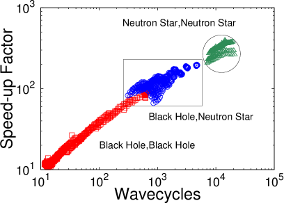
(a)

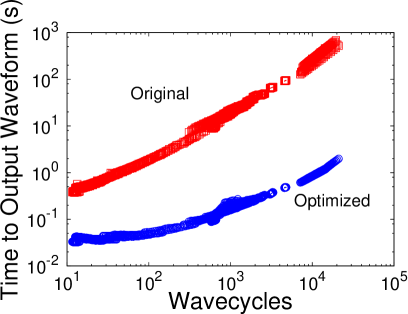
(b)

Figure 1: Performance Benchmarks: Left panel: Speed-up factor for (fully) Optimized versus Original SEOBNRv2, considering key compact binary systems of interest to Advanced LIGO. Right panel: Total time required to produce SEOBNRv2 waveforms for the same compact binary systems (in seconds). The ratio of the top curve to the bottom curve in the right panel for a given scenario is equivalent to the speed-up factor of the left panel. Initial parameters for waveforms are as specified in Table 2, with start frequency of 10 Hz and output sample rate set to 16,384 Hz. Performance was measured on a computer with an Intel i7-4790 CPU and 16 GB of RAM.

$\begin{aligned} \begin{subfigure}{130.08731pt}\includegraphics[width=420.61192pt]{./plotsv5/SpeedUp_1_Plot.eps}\@@toccaption{{\lx@tag[ ]{{(a)}}{}}}\@@caption{{\lx@tag[ ]{{\small(a)}}{\small}}}\end{subfigure}\hskip 4.26773pt\begin{subfigure}{130.08731pt}\includegraphics[width=420.61192pt]{./plotsv5/SpeedUp_2_Plot.eps}\@@toccaption{{\lx@tag[ ]{{(b)}}{}}}\@@caption{{\lx@tag[ ]{{\small(b)}}{\small}}}\end{subfigure}\\ \begin{subfigure}{130.08731pt}\includegraphics[width=420.61192pt]{./plotsv5/SpeedUp_3_Plot.eps}\@@toccaption{{\lx@tag[ ]{{(c)}}{}}}\@@caption{{\lx@tag[ ]{{\small(c)}}{\small}}}\end{subfigure}\hskip 4.26773pt\begin{subfigure}{130.08731pt}\includegraphics[width=420.61192pt]{./plotsv5/SpeedUp_4_Plot.eps}\@@toccaption{{\lx@tag[ ]{{(d)}}{}}}\@@caption{{\lx@tag[ ]{{\small(d)}}{\small}}}\end{subfigure}\end{aligned}$

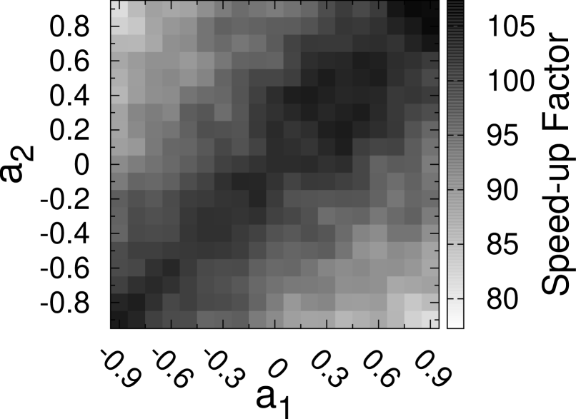
(a)

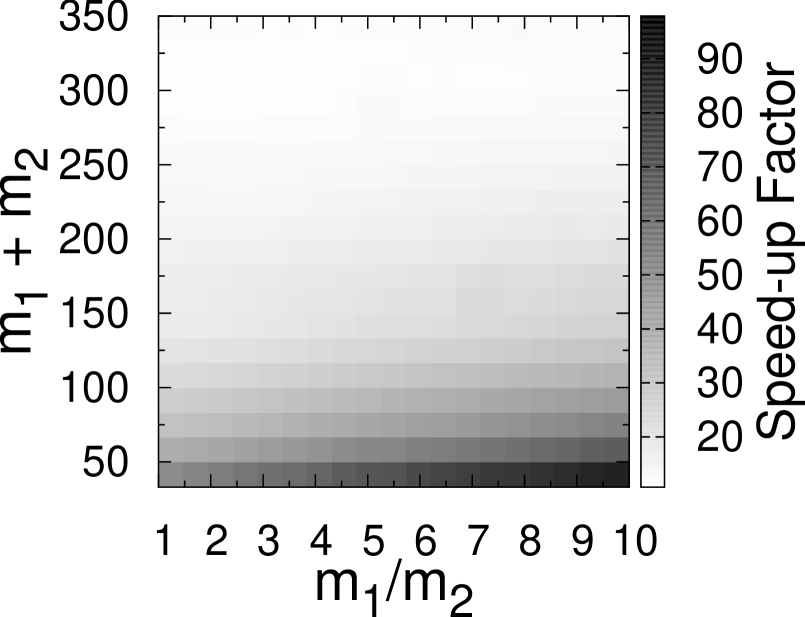
(b)

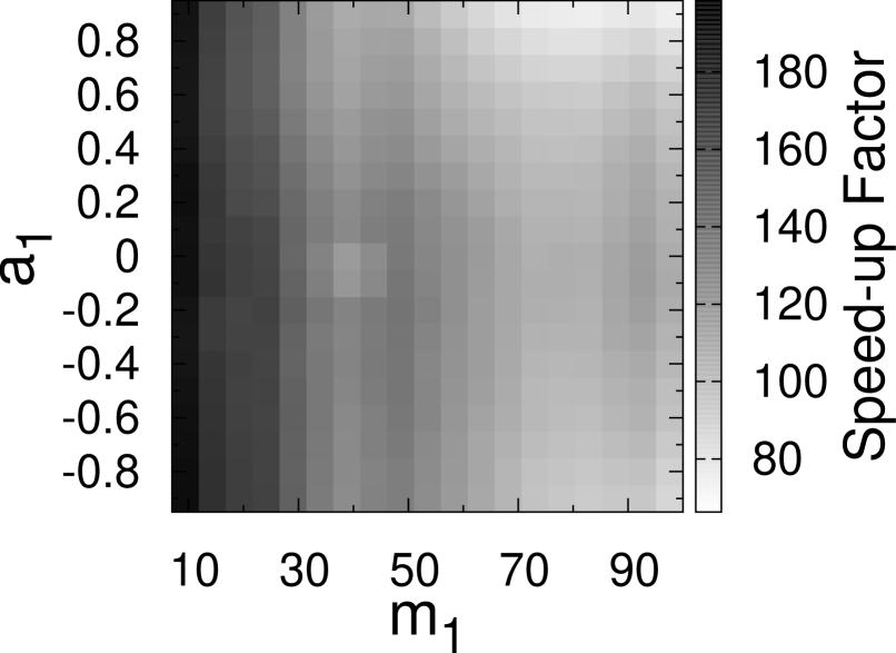
(c)

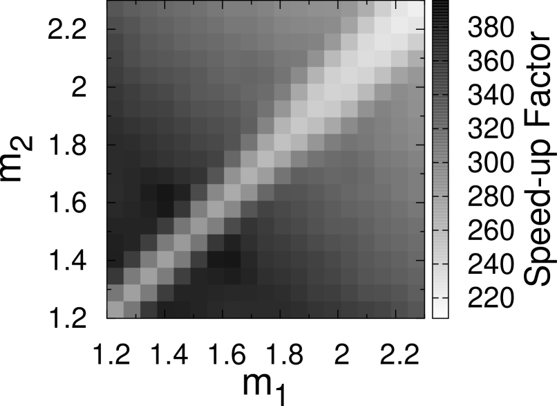
(d)

Figure 2: Speed-ups over parameter spaces: Measured speed-up factors across SEOBNRv2 parameter space, where speed-up factor is defined as the ratio of run-time of the original SEOBNRv2 code to our optimized version. Note that these results use exactly the same data as in Fig. 1. The shading of each of the 1,600 pixels in these panels corresponds to the measured speed-up factor for one of the 1,600 cases specified in Table 2, with darker shading corresponding to larger speed-ups. Each panel corresponds to a different physical scenario, with the top-left denoting BHB_s, top-right BHB_m, bottom-left BHNS, and bottom-right DNS.

Physical Scenario	Error Maxima						Average Speed-up
	$||\Delta_{\phi}||_{A}$	$Q_{1}$	$Q_{2}$	$||\Delta_{\mathcal{A}}||_{A}$	$Q_{1}$	$Q_{2}$	$\mathcal{S}$
${\rm BHB_{S}}$	0.00735	-0.850	-0.750	-4.01	-0.650	0.050	96.4
${\rm BHB_{M}}$	0.00523	4.32	167.	-3.81	1.94	333.	53.7
${\rm BHNS}$	0.00790	41.3	0.950	-4.30	26.6	0.750	145
${\rm DNS}$	0.00465	1.66	1.66	-4.09	1.20	1.49	322

Table 3: Maximum Errors and Overall Speed-ups: Summary of results of parameter survey (as specified in Table 2). $||\Delta_{\phi}||_{A}$ and $||\Delta_{\mathcal{A}}||_{A}$ denote the maximum amplitude weighted amplitude and phase errors (Eqs. 2 and 3). $Q_{1}$ and $Q_{2}$ (See Table 2) are the variable parameters resulting in the maximum $||\Delta_{\phi}||_{A}$ and $||\Delta_{\mathcal{A}}||_{A}$. $\mathcal{S}$ is the weighted average speed-up for each scenario (Eq. 1).

3.2 Code Validation Tests

We conclude that our performance speed-ups are substantial, but unless we can guarantee that the optimized code generates waveforms that agree as well as numerically possible with the original (i.e., to roundoff-error), then we could not be confident that we did not introduce some error in the code. Defining quantities most useful for such error analysis was a difficult task, as with the original SEOBNRv2 code, perturbations at the 15th significant digit in initial parameters could, e.g., generate amplitude differences of order unity at the end of the ringdown, where the amplitude was of order $10^{-6}$ the maximum amplitude, yet at all other points the amplitudes would agree to many ($\sim 6+$) significant digits. To mitigate this effect, we compute the amplitude-weighted relative amplitude error:

$$||\Delta A||_{A}=\frac{\sum_{t}A_{t}\log_{10}(|{A_{1}}_{t}-{A_{2}}_{t}|/|{A_{1}}_{t}|)}{\sum_{t}|A_{t}|}\,,$$ (2)

where ${A_{1}}_{t}$ and ${A_{2}}_{t}$ are the two compared amplitudes at time $t$ with ${A_{1}}_{t}$ taken to be the larger of the two amplitudes and ${A_{t}}$ chosen to be the amplitude at time $t$ of one waveform, consistently. Similarly for phase, the amplitude-weighted phase error was computed,

$$||\Delta\theta||_{A}=\frac{\sum_{t}|A_{t}({\theta_{1}}_{t}-{\theta_{2}}_{t})|}{\sum_{t}|A_{t}|}$$ (3)

where ${\theta_{1}}_{t}$ and ${\theta_{2}}_{t}$ were the compared phases, and $A_{t}$ is the same as in the amplitude error calculation.

The algorithm to compare two waveforms works as follows. The waveforms output by LALSuite are output with uniform timesteps such that the time of peak amplitude is chosen to be $t=0$ seconds. If the initial parameters are perturbed infinitesimally (i.e., at the 15th significant digit), or even if different compilers/compiler flags are used to generate the trusted, un-optimized SEOBNRv2 executable, then this peak shifts slightly, shifting the position of t=0 slightly; this sometimes changes the number of data points prior to the peak. As a result, an additional point or two may be added to the start of the waveform with the later peak. Let’s call this waveform A. Naturally, the tail of waveform A will generally truncate a couple of points earlier than the other waveform (waveform B).

So the first step in our error analysis removes data points from the start of waveform A until the initial time is within a single timestep of the start of waveform B. The same number of data points are removed from the tail of waveform B.

Since an overall small time shift may still be present between the waveforms, the amplitudes and phases of one waveform are quadratically interpolated to the moments in time provided by the other waveform. Once the amplitude of either waveform dropped to zero, the times of the last two nonzero amplitudes and all times which followed were truncated. Finally, the amplitude and phase errors (Eqs. 2 and 3) were computed.

Figure 3 shows that the phase and amplitude differences between LALSuite’s SEOBNRv2 and our SEOBNRv2_opt (Eqs. 2 and 3) are stochastically distributed across our 1,600-point parameter survey. To measure the magnitude of roundoff errors in the original code, we computed the same differences, comparing instead the original code with itself but with a small, 15th-significant-digit perturbation to the input parameters (e.g., $m_{1}\to m_{1}(1+10^{-15})$). I.e., we measure the expected roundoff errors by perturbing the input parameters by a small multiple of double-precision machine epsilon.

The overlap between the expected roundoff error and the error in the optimized code is striking, consistent with the explanation that differences between the optimized and un-optimized codes are completely due to roundoff error.

We focused our efforts on computing amplitude and phase errors in the region near merger, because, as shown in Fig. 4 this region contains the largest phase errors. Fig. 4 also demonstrates that no significant phase difference had accrued up to this region. Regardless, to be absolutely certain in our results, we repeated our full amplitude and phase discrepancy analysis on data using only the first 10,000 output times of each waveform as well, and precisely the same degree of overlap between optimized and un-optimized waveform amplitude and phases was observed.

We summarize in Table 3 the cases with the largest discrepancies in amplitude and phase between the optimized and un-optimized codes, for each of the four scenarios. Notice that there is no clear pattern in worst-case parameters, consistent with the stochastic nature of phase and amplitude errors observed in Fig. 3. In addition, we observe in the worst case discrepancies in phase of roughly 0.008 rad and relative amplitude of $10^{-3.8}$.

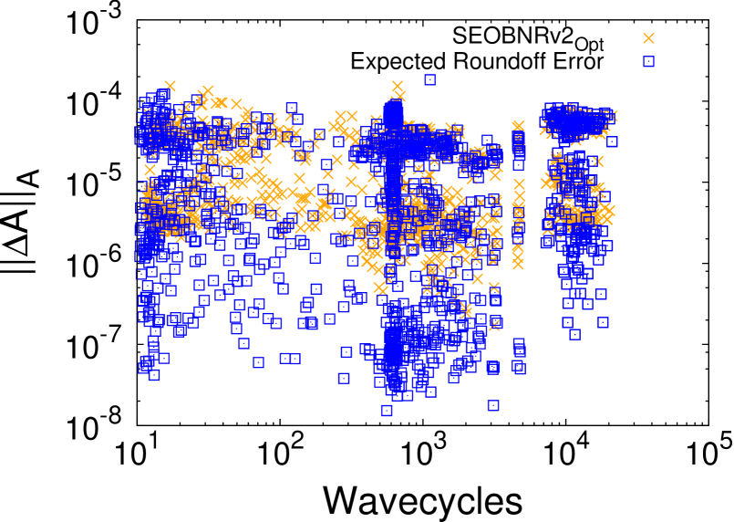
(a)

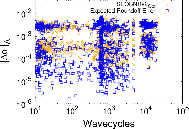
(b)

Figure 3: roundoff Error vs Optimization Mismatch: The amplitude left and phase right errors vs wavecycles, compared to the error caused by an order-machine-epsilon perturbation in one of the masses (Roundoff Error), for all of the surveyed parameter space. Both panels demonstrate much overlap between these quantities.

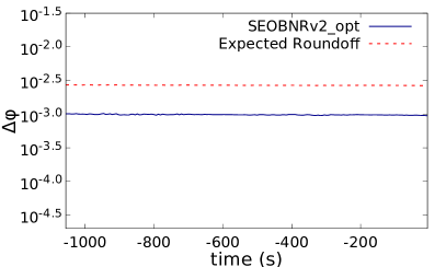
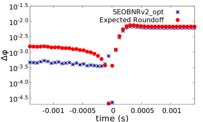
Figure 4: Phase Differences vs Time: Shown is a typical example of the phase differences ($\Delta\phi$) near merger (right panel) and before (left panel), between a waveform generated by SEOBNRv2 and a waveform generated by SEOBNRv2_opt using the same input parameters, as well as the phase differences between the same waveform generated by SEOBNRv2 code and that generated by SEOBNRv2 with input parameters were perturbed to the order of $10^{-15}$. This value is taken to be the expected roundoff error. This system corresponds to a nonspinning DNS system with masses $1.258$ and $1.489$. Notice that the phase differences are roughly constant until near merger.

3.3 Improved Sensitivity to Initial Parameters

The SEOBNR codes are designed to read in start frequency and intrinsic binary parameters such as initial masses and spins. The codes then use these parameters to generate initial conditions for radius $r$, radial momentum $p_{r}$, and $\phi$-component of momentum $p_{\phi}$ for the system, which are required inputs to the SEOBNR Hamiltonian equations of motion. In computing Hamiltonian input quantities consistent with the initial parameters, the SEOBNR codes evaluate finite difference derivatives of the Hamiltonian.

Unfortunately, it is well known that finite difference derivatives can be prone to enormous roundoff errors, which act to enormously amplify small perturbations in chosen initial binary parameters, yielding an observable effect on amplitude and phase of resulting waveforms. For example, if the initial mass of a single binary component is perturbed by anywhere from one part in $10^{15}$ to one part in $10^{8}$, the resulting perturbation in $p_{\phi}$ input into the Hamiltonian will be stochastic, with perturbation amplitude fixed at one part in $10^{9}$, thus making SEOBNRv2 completely incapable of exploring initial mass perturbations beyond the eighth significant digit.

Such sensitivities to initial conditions are illustrated in Fig. 5, where we plot the change in these Hamiltonian input parameters as a logarithmic function of perturbation added to one of the binary masses $m_{1}$. Notice that when we replace the finite-difference derivatives of the SEOBNRv2 Hamiltonian with their exact expressions, computed using C-code generated by Mathematica, the sensitivity to small perturbations in initial conditions is improved by several orders of magnitude. We anticipate these improvements in accuracy will have a positive impact on using SEOBNR for PE algorithms that depend on taking small steps through parameter space, such as Fisher-matrix-based estimates of uncertainties in the large signal limit.

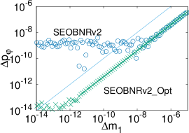
(a)

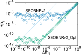
(b)

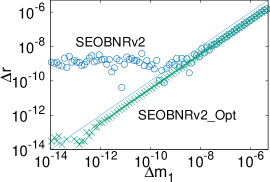
(c)

Figure 5: Initial data sensitivity mass perturbation: The dependence of the initial values of $p_{r}$ and $p_{\phi}$ on the mass, $m_{1}$ of one compact object of the system, in both the original code and the optimized version. $\Delta p_{\phi}$,$\Delta p_{r}$, and $\Delta r$ are the differences in the initial values of $p_{\phi}$,$p_{r}$, and $r$ when $m_{1}=1.4M_{\odot}$ and when $m_{1}=m_{1}+\Delta m_{1}$. In each case, the other mass, $m_{2}$, of the system was fixed at $14.001M_{\odot}$. The SEOBNRv2_opt line, in each case, extends to about 5 orders of magnitude lower than the SEOBNRv2 line, before roundoff error becomes significant. The solid blue black diagonal line is the line of equal change in $m_{1}$ and the initial value.

4 Conclusions and Future Work

In preparation for the 8-dimensional, precessing SEOBNRv3 (v3) model’s final incorporation into LALSuite, we have worked to increase the performance of the 4-dimensional SEOBNRv2 (v2) by $\sim$300x (Eq 1 and Table 3), so that PE can now be performed directly with SEOBNRv2 within weeks to months using standard, serial-processing MCMC techniques, which could be reduced to days or weeks with minimal parallelization. Our optimization strategies have been shown to dramatically reduce the SEOBNRv2 run-time and over-sensitivity to initial conditions, while maintaining amplitude-weighted phase agreement with the original code to within 0.00790 rad (Table 3), which is entirely dominated by roundoff errors. The work discussed in this paper is hoped to not only assist MCMC parameter estimation but be useful to others in the community who cannot use pre-optimized SEOBNR codes due to their slow speeds (e.g., the generation of stochastic template banks [33]).

Some of our optimizations have already been applied to the SEOBNRv3 code within LALSuite, leading to speed-ups of around 15x over its original version. We anticipate that overall speed-ups of $\sim$300x of v3 are likely once the remainder of our v2 optimizations have been incorporated, as the codes are identical in structure and inefficiencies.

As we work to optimize SEOBNRv3, the resulting v3 code can be viewed as a stopgap for v3-based PE while efficient new 8-D ROM strategies are invented, which may be capable of far faster waveform generation than even a $\sim$300x-optimized SEOBNRv3 code.

Excitingly, we do not believe even our optimized SEOBNRv2 code is particularly efficient and are confident that significant, $\sim$100x optimizations are still possible (leading to overall speed-up factors of $\sim$10,000x, over the original LALSuite SEOBNRv2 and v3 codes). Though the release of SEOBNRv3 marks the end of our efforts toward optimizing SEOBNRv2, we are eager to apply new optimization ideas to v3, once all of the v2 optimizations have been incorporated. With our planned optimizations of v3, a timely interpretation of an observed gravitational wave using precessing SEOBNR models directly may be within reach.

References

References

- [1] The LIGO Scientific Collaboration, J. Aasi, B. P. Abbott, R. Abbott, T. Abbott, M. R. Abernathy, K. Ackley, C. Adams, T. Adams, P. Addesso, and et al. Advanced LIGO. Classical and Quantum Gravity, 32(7):074001, April 2015.
- [2] F. Acernese and et al. Advanced Virgo: a 2nd generation interferometric gravitational wave detector. Classical and Quantum Gravity, 32:024001, May 2015.
- [3] B. P. Abbott, R. Abbott, F. Acernese, R. Adhikari, P. Ajith, B. Allen, G. Allen, M. Alshourbagy, R. S. Amin, S. B. Anderson, and et al. An upper limit on the stochastic gravitational-wave background of cosmological origin. Nature, 460:990–994, August 2009.
- [4] B. P. Abbott, R. Abbott, T. D. Abbott, M. R. Abernathy, F. Acernese, K. Ackley, C. Adams, T. Adams, P. Addesso, R. X. Adhikari, and et al. Observation of Gravitational Waves from a Binary Black Hole Merger. Physical Review Letters, 116(6):061102, February 2016.
- [5] J. Veitch, V. Raymond, B. Farr, W. Farr, P. Graff, S. Vitale, B. Aylott, K. Blackburn, N. Christensen, M. Coughlin, W. Del Pozzo, F. Feroz, J. Gair, C.-J. Haster, V. Kalogera, T. Littenberg, I. Mandel, R. O’Shaughnessy, M. Pitkin, C. Rodriguez, C. Röver, T. Sidery, R. Smith, M. Van Der Sluys, A. Vecchio, W. Vousden, and L. Wade. Parameter estimation for compact binaries with ground-based gravitational-wave observations using the LALInference software library. Phys. Rev. D, 91(4):042003:1–25, 2015.
- [6] B. Szilágyi, J. Blackman, A. Buonanno, A. Taracchini, H. P. Pfeiffer, M. A. Scheel, T. Chu, L. E. Kidder, and Y. Pan. Approaching the Post-Newtonian Regime with Numerical Relativity: A Compact-Object Binary Simulation Spanning 350 Gravitational-Wave Cycles. Physical Review Letters, 115(3):031102, July 2015.
- [7] M. Hannam, P. Schmidt, A. Bohé, L. Haegel, S. Husa, F. Ohme, G. Pratten, and M. Pürrer. Simple Model of Complete Precessing Black-Hole-Binary Gravitational Waveforms. Physical Review Letters, 113(15):151101, 2014.
- [8] S. Husa, S. Khan, M. Hannam, M. Pürrer, F. Ohme, X. Jiménez Forteza, and A. Bohé. Frequency-domain gravitational waves from non-precessing black-hole binaries. I. New numerical waveforms and anatomy of the signal. ArXiv e-prints, 1508.07250, 2015. preprint.
- [9] S. Khan, S. Husa, M. Hannam, F. Ohme, M. Pürrer, X. Jiménez Forteza, and A. Bohé. Frequency-domain gravitational waves from non-precessing black-hole binaries. II. A phenomenological model for the advanced detector era. ArXiv e-prints, 1508.07253, 2015. preprint.
- [10] P. Kumar, T. Chu, H. Fong, H. P. Pfeiffer, M. Boyle, D. A. Hemberger, L. E. Kidder, M. A. Scheel, and B. Szilagyi. Accuracy of binary black hole waveform models for aligned-spin binaries. ArXiv e-prints, January 2016.
- [11] A. Taracchini, A. Buonanno, Y. Pan, T. Hinderer, M. Boyle, D. A. Hemberger, L. E. Kidder, G. Lovelace, A. H. Mroué, H. P. Pfeiffer, M. A. Scheel, B. Szilágyi, N. W. Taylor, and A. Zenginoglu. Effective-one-body model for black-hole binaries with generic mass ratios and spins. Phys. Rev. D, 89(6):061502:1–6, March 2014.
- [12] A. Buonanno, Y. Pan, J. G. Baker, J. Centrella, B. J. Kelly, S. T. McWilliams, and J. R. van Meter. Approaching faithful templates for nonspinning binary black holes using the effective-one-body approach. Phys. Rev. D, 76(10):104049:1–15, 2007.
- [13] T. Damour, A. Nagar, M. Hannam, S. Husa, and B. Brügmann. Accurate effective-one-body waveforms of inspiralling and coalescing black-hole binaries. Phys. Rev. D, 78(4):044039:1–24, 2008.
- [14] T. Damour and A. Nagar. Improved analytical description of inspiralling and coalescing black-hole binaries. Phys. Rev. D, 79(8):081503:1–5, 2009.
- [15] Y. Pan, A. Buonanno, L. T. Buchman, T. Chu, L. E. Kidder, H. P. Pfeiffer, and M. A. Scheel. Effective-one-body waveforms calibrated to numerical relativity simulations: Coalescence of nonprecessing, spinning, equal-mass black holes. Phys. Rev. D, 81(8):084041:1–15, 2010.
- [16] N. Yunes, A. Buonanno, S. A. Hughes, M. C. Miller, and Y. Pan. Modeling Extreme Mass Ratio Inspirals within the Effective-One-Body Approach. Phys. Rev. Lett., 104(9):091102:1–4, 2010.
- [17] Y. Pan, A. Buonanno, M. Boyle, L. T. Buchman, L. E. Kidder, H. P. Pfeiffer, and M. A. Scheel. Inspiral-merger-ringdown multipolar waveforms of nonspinning black-hole binaries using the effective-one-body formalism. Phys. Rev. D, 84(12):124052:1–42, 2011.
- [18] A. Taracchini, Y. Pan, A. Buonanno, E. Barausse, M. Boyle, T. Chu, G. Lovelace, H. P. Pfeiffer, and M. A. Scheel. Prototype effective-one-body model for nonprecessing spinning inspiral-merger-ringdown waveforms. Phys. Rev. D, 86(2):024011:1–20, 2012.
- [19] T. Damour, A. Nagar, and S. Bernuzzi. Improved effective-one-body description of coalescing nonspinning black-hole binaries and its numerical-relativity completion. Phys. Rev. D, 87(8):084035:1–42, 2013.
- [20] Y. Pan, A. Buonanno, A. Taracchini, L. E. Kidder, A. H. Mroué, H. P. Pfeiffer, M. A. Scheel, and B. Szilágyi. Inspiral-merger-ringdown waveforms of spinning, precessing black-hole binaries in the effective-one-body formalism. Phys. Rev. D, 89(8):084006, April 2014.
- [21] A. Nagar, T. Damour, C. Reisswig, and D. Pollney. Energetics and phasing of nonprecessing spinning coalescing black hole binaries. ArXiv e-prints, 1506.08457, June 2015. preprint.
- [22] E. Barausse and A. Buonanno. Extending the effective-one-body Hamiltonian of black-hole binaries to include next-to-next-to-leading spin-orbit couplings. Phys. Rev. D, 84(10):104027, November 2011.
- [23] LALSuite Homepage. http://software.ligo.org/docs/lalsuite/lalsuite/.
- [24] M. Pürrer. Frequency-domain reduced order models for gravitational waves from aligned-spin compact binaries. Class. Quantum Grav., 31(19):195010:1–36, 2014.
- [25] D. A. Brown, I. Harry, A. Lundgren, and A. H. Nitz. Detecting binary neutron star systems with spin in advanced gravitational-wave detectors. Phys. Rev. D, 86(8):084017, October 2012.
- [26] S. E. Field, C. R. Galley, J. S. Hesthaven, J. Kaye, and M. Tiglio. Fast Prediction and Evaluation of Gravitational Waveforms Using Surrogate Models. Phys. Rev. X, 4(3):031006:1–21, 2014.
- [27] M. Pürrer. Frequency domain reduced order model of aligned-spin effective-one-body waveforms with generic mass-ratios and spins. ArXiv e-prints, 1512.02248, December 2015. preprint.
- [28] B. Farr, C. P. L. Berry, W. M. Farr, C.-J. Haster, H. Middleton, K. Cannon, P. B. Graff, C. Hanna, I. Mandel, C. Pankow, L. R. Price, T. Sidery, L. P. Singer, A. L. Urban, A. Vecchio, J. Veitch, and S. Vitale. Parameter estimation on gravitational waves from neutron-star binaries with spinning components. ArXiv e-prints, 1508.05336, 2015. preprint.
- [29] Richard M. Stallman and GCC DeveloperCommunity. Using The Gnu Compiler Collection. 51 Franklin Street, Fifth Floor, Boston, MA 02110-1301 USA, 2015.
- [30] Intel. User and Reference Guide for the Intel® C++ Compiler 15.0, 2014. https://software.intel.com/en-us/compiler_15.0_ug_c.
- [31] Wolfram Research, Inc. Mathematica 10.0. Champaign, Illinois, 2014. https://www.wolfram.com.
- [32] Brian Gough. GNU Scientific Library Reference Manual - Third Edition. Network Theory Ltd., 3rd edition, 2009. http://www.gnu.org/software/gsl/.
- [33] C. Capano, I. Harry, S. Privitera, and A. Buonanno. Implementing a search for gravitational waves from non-precessing, spinning binary black holes. ArXiv e-prints, February 2016.