Identifier Namespaces in Mathematical Notation

Master Thesis

by

Alexey Grigorev

Submitted to the Faculty IV, Electrical Engineering and Computer Science Database Systems and Information Management Group in partial fulfillment of the requirements for the degree of

Master of Science in Computer Science

as part of the Erasmus Mundus IT4BI programme

at the

Technische Universität Berlin

July 31, 2015

Thesis Advisors:

Moritz Schubotz
Juan Soto

Thesis Supervisor:

Prof. Dr. Volker Markl

Eidesstattliche Erklärung

Ich erkläre an Eides statt, dass ich die vorliegende Arbeit selbstständig verfasst, andere als die angegebenen Quellen/Hilfsmittel nicht benutzt, und die den benutzten Quellen wörtlich und inhaltlich entnommenen Stellen als solche kenntlich gemacht habe.

Statutory Declaration

I declare that I have authored this thesis independently, that I have not used other than the declared sources/resources, and that I have explicitly marked all material which has been quoted either literally or by content from the used sources.

Abstract

In Computer Science, namespaces help to structure source code and organize it into hierarchies. Initially, the concept of namespaces did not exist for programming languages, and programmers had to manage the source code themselves to ensure there were no name conflicts. However, nowadays, namespaces are adopted by the majority of modern programming languages.

The concept of namespaces is beneficial for mathematics as well: In mathematics, short one-symbol identifiers are very common, and the meaning of these identifiers is hard to understand immediately. By introducing namespaces to mathematics, we will be able to organize mathematical identifiers. Also, mathematicians will also benefit from a hierarchical organization of knowledge in the same way programmers do. In addition, the structure will make it easier to understand the meaning of each identifier in a document.

In this thesis, we look at the problem of assigning each identifier of a document to a namespace. At the moment, there does not exist a special dataset where all identifiers are grouped to namespaces, and therefore we need to create such a dataset ourselves.

Namespaces are hard to prepare manually: building them requires a lot of time and effort. However, it can be done automatically, and we propose a method for automatic namespace discovery from a collection of documents.

To do that, we need to find groups of documents that use identifiers in the same way. This can be done with cluster analysis methods. We argue that documents can be represented by the identifiers they contain, and this approach is similar to representing textual information in the Vector Space Model. Because of this, we can apply traditional document clustering techniques for namespace discovery.

To evaluate the results, we use the category information, and look for pure ‘‘namespace-defining’’ clusters: clusters where all documents are from the same category. In the experiments, we look for algorithms that discover as many namespace-defining clusters as possible.

Because the problem is new, there is no gold standard dataset, and it is hard to evaluate the performance of our method. To overcome it, we first use Java source code as a dataset for our experiments, since it contains the namespace information. We verify that our method can partially recover namespaces from source code using only information about identifiers.

The algorithms are evaluated on the English Wikipedia, and the proposed method can extract namespaces on a variety of topics. After extraction, the namespaces are organized into a hierarchical structure by using existing classification schemes such as MSC, PACS and ACM. We also apply it to the Russian Wikipedia, and the results are consistent across the languages.

To our knowledge, the problem of introducing namespaces to mathematics has not been studied before, and prior to our work there has been no dataset where identifiers are grouped into namespaces. Thus, our result is not only a good start, but also a good indicator that automatic namespace discovery is possible.

Zusammenfassung

Namespaces in Informatik helfen um den Quellcode zu organisieren. Namespaces sind auch für Mathematik vorteilhaft. Durch die Einfьhrung von Namespaces in der Mathematik, kann mann mathematische Identifikatoren in einer hierarchy organisieren.

In dieser Masterarbeit betrachten wir das Problem der Zuordnung jeder Identifikator eines Dokuments zu einem Namespaces. Im Moment gibt es keine spezielle Datenmenge in der alle Mathematische Identifikatoren zu Namespaces zugeordnet sind. Deshalb müssen wir eine Datenmenge selbst erstellen. Wir schlagen eine automatisierte methode vor für die Entdeckung von der Zuordnung von Namespaces zu Identifikatoren aus einer Sammlung von Dokumenten.

Um dies zu erreichen, müssen wir Gruppen von Dokumenten finden, die Identifikatoren in der gleichen Weise verwenden. Das kann mit Clustering-Algorithmen durchgefьhrt werden. Wir schlagen vor dass Dokumente repräsentiert werden können durch die Identifikatoren die sie enthalten. Dieser Ansatz ist ähnlich zu der Abbildung von Textinformationen in dem Vektorraummodell. Aus diesem Grund können wir traditionelle Dokument Clustering-Algorithmen für Namespace Entdeckung gelten.

Um die Ergebnisse zu bewerten, verwenden wir die Kategorieinformationen, und suchen wir nach reinen ‘‘namespace-definierenden’’ Cluster: Cluster, in dem alle Dokumente zu der gleichen Kategorie gehören. In die Experimenten suchen wir nach Algorithmen, die so viele reine Cluster wie mцglich entdecken.

Die Algorithmen sind auf der Englischen Wikipedia ausgewertet. Unsere Methode kann Namespaces auf einer Vielzahl von Themen extrahieren. Nach der Extraktion, organisieren wir die Namespaces in einer Hierarchie. Wir setzen unsere Methode auch auf der Russischen Wikipedia und finden änlische Ergebnisse. Unser Ergebnis zeigt, dass die automatische Namespaces Entdeckung möglich ist.

1 Introduction

1.1 Motivation

In computer science, a namespace refers to a collection of terms that are grouped, because they share functionality or purpose, typically for providing modularity and resolving name conflicts [1]. For example, XML uses namespaces to prefix element names to ensure uniqueness and remove ambiguity between them [2], and the Java programming language uses packages to organize classes into namespaces for modularity [3].

In this thesis, we extend the notion of namespaces to mathematical formulae. In mathematics, there is a convention of choosing identifier names in mathematical notation [4]. Because of the notation, when people write ‘‘$E=mc^{2}$’’, the meaning of this expression is recognized among scientists. However, the same identifier may be used in different areas, but denote different things: For example, ‘‘$E$ ’’ may refer to ‘‘energy’’, ‘‘expected value’’ or ‘‘elimination matrix’’, depending on the domain of the article. We can compare this problem with the problem of name collision in computer science and introduce namespaces of identifiers in mathematical notation to overcome it.

In this work we aim to discover namespaces of identifiers in mathematical notation. However, the notation only exists in the documents where it is used, and it does not exist in isolation. It means that the identifer namespaces should be discovered from the documents with mathematical formulae. Therefore, the goal of this work is to automatically discover a set of identifier namespaces given a collection of documents.

We expect the namespaces to be meaningful, in the sense that they can be related to real-world areas of knowledge, such as physics, linear algebra or statistics.

Once such namespaces are found, they can give good categorization of scientific documents based on formulas and notation used in them. We believe that this may facilitate better user experience: when learning a new area it will help the users familiarize with the notation faster. Additionally, it may also help to locate the usages of a particular identifier and refer to other documents where the identifier is used.

Namespaces also give a way to avoid ambiguity. If we refer to an identifier from a particular namespace, then it is clear what the semantic meaning of this identifier. For example, if we say that ‘‘$E$ ’’ belongs to a namespaces about physics, it gives additional context and makes it clear that ‘‘$E$ ’’ means ‘‘energy’’ rather than ‘‘expected value’’.

Finally, using namespaces is beneficial for relating identifiers to definitions. Thus, as an application of namespaces, we can use them for better definition extraction. It will help to overcome some of the current problems in this area, for example, the problem of dangling identifiers – identifiers that are used in formulas but never defined in the document [5]. Such identifiers may be defined in other documents that share the same namespace, and thus we can take the definition from the namespace and assign it to the dangling identifier.

1.2 Thesis Outline

The thesis is organizes as follows:

Chapter 2 – Background and Related Work

In this chapter, we do a survey of the related work. We discuss how namespaces are used in Computer Science. Secondly, we review how definitions for identifiers used in mathematical formulae can be extracted from the natural language text around the formulae. Finally, we review the Vector Space Model – a way of transforming texts to vectors, and then discuss how these vectors can be clustered.

Chapter 3 – Namespace Discovery

In chapter 3 we introduce the problem of namespaces in mathematical notation, discuss its similarities with namespaces in Computer Science, and propose an approach to namespace discovery by using document clustering techniques. We also extend the Vector Space Model to represent identifiers and suggest several ways to incorporate definition information to the vector space.

Chapter 4 – Implementation

Chapter 4 describes how the proposed approach is implemented. It includes the description of the data sets for our experiments, and the details of implementation of definition extraction and document cluster analysis algorithms. Additionally, we propose a way of converting document clusters to namespaces.

Chapter 5 – Evaluation

In chapter 5, we describe the parameter selection procedure, and we present the results of the best performing method. Once the clusters are discovered, they are mapped to a hierarchy, and we summarize our findings by analyzing the most frequent namespaces and most frequent identifier-definition relations in these namespaces.

Chapter 6 – Conclusions

Chapter 6 summarizes the findings.

Chapter 7 – Outlook and Future Work

Finally, in chapter 7 we discuss the possible areas of improvements. We conclude this chapter by identifying the questions that are not resolved and present challenges for future research on identifier namespace discovery.

2 Background and Related Work

In this chapter we explain the related work: we give a short overview about existing approaches and relevant methods.

First, we describe the concept of a namespace from the Computer Science point of view in section 2.1. Then we discuss how identifier definitions can be extracted, and for that we first introduce Part-of-Speech Tagging and its application to mathematical texts in section 2.2, and then review the extraction methods in section 2.3.

Next, section 2.4 describes the Vector Space Model, a traditional way of representing a collection of documents as vectors, and then section 2.5 reviews common similarity and distance functions that are useful for document clustering.

Finally, document clustering techniques are described in section 2.6, and the Latent Semantic Analysis method for revealing semantic information from the document corpus is in section 2.7.

2.1 Namespaces in Computer Science

In computer science, a namespace refers to a collection of terms that are grouped because they share functionality or purpose, typically for providing modularity and resolving name conflicts [1].

Example 1. Namespaces are used in XML (eXtensible Markup Language), which is a framework for defining markup languages [6]. However, different XML languages may use the same names for elements and attributes. For example, consider two XML languages: XHTML for specifying the layout of web pages, and some XML language for describing furniture. Both these languages have the <table> elements there, in XHTML table is used to present some data in a tabular form, while the second one uses it to describe a particular piece of furniture in the database.

The <table> elements have very different semantics in these languages and there should be a way to distinguish between these two elements. In XML this problem is solved with XML namespaces [2]: the namespaces are used to ensure the uniqueness of attributes and resolve ambiguity. It is done by binding a short namespace alias with some uniquely defined URI (Unified Resource Identifier), and then appending the alias to all attribute names that come from this namespace. In the example above, we can bind an alias h with XHTML’s URI http://www.w3.org/TR/xhtml1 and then use <h:table> to refer to XHTML’s table. Likewise, in the furniture database language the element names can be prepended with a prefix d, where d is bound to some URI, e.g. http://www.furniture.de/2015/db.

Example 2. Namespaces are also used in programming languages for organizing variables, procedures and other identifiers into groups and for resolving name collisions. In programming languages without namespaces the programmers have to take special care to avoid naming conflicts. For example, in the PHP programming language prior to version 5.3 [7] there is no notion of namespace, and the namespaces have to be emulated to ensure that the names are unique, and Zend_Search_Lucene_Analysis_Analyzer and other long names is the result.

Other programming languages have the notion of namespaces built in from the very first versions. For example, the Java programming language [3] uses packages to organize identifiers into namespaces, and packages solve the problem of ambiguity. For example, in the standard Java API there are two classes with the name Date: one in the package java.util and another in the package java.sql. To be able to distinguish between them, the classes are referred by their fully qualified name: an unambiguous name that uniquely specifies the class by combining the package name with the class name. Thus, to refer to a particular Date class in Java java.util.Date or java.sql.Date should be used.

It is not always convenient to use the fully qualified name in the code to refer to some class from another package. Therefore in Java it is possible to import the class by using the import statement which associates a short name alias with its fully qualified name. For example, to refer to java.sql.Date it is possible to import it by using import java.sql.Date and then refer to it by the alias Date in the class [3].

Although there are no strict rules about how to organize the classes into packages, it is a good software design practice to put related objects into the same namespace and by doing this achieve better modularity. There are design principles that tell software engineers how to best organize the source code: classes in a well designed system should be grouped in such a way that namespaces exhibit low coupling and high cohesion [8]. Coupling describes the degree of dependence between namespaces, and low coupling means that the interaction between classes of different namespaces should be as low as possible. Cohesion, on the other hand, refers to the dependence within the classes of the same namespace, and the high cohesion principle says that the related classes should all be put together in the same namespace.

2.2 Math-aware POS tagging

Part-of-Speech Tagging (POS Tagging) is a typical Natural Language Processing task which assigns a POS Tag to each word in a given text [9]. While the POS Tagging task is mainly a tool for text processing, it can also be applicable to scientific documents with mathematical expressions, and can be adjusted to dealing with formulae [10] [5].

A POS tag is an abbreviation that corresponds to some part of speech. Penn Treebank POS Scheme [11] is a commonly used POS tagging scheme which defines a set of part-of-speech tags for annotating English words. For example, JJ is an adjective (‘‘big’’), RB as in adverb, DT is a determiner (‘‘a’’, ‘‘the’’), NN is a noun (‘‘corpus’’) and SYM is used for symbols (‘‘$>$’’, ‘‘$=$’’).

However the Penn Treebank scheme does not have special tags for mathematics, but it is flexible enough and can be extended to include additional tags. For example, we can include a math-related tag MATH. Usually it is done by first applying traditional POS taggers (like Stanford CoreNLP [12]), and then refining the results by re-tagging math-related tokens of text as MATH [10].

For example, consider the following sentence: ‘‘The relation between energy and mass is described by the mass-energy equivalence formula $E=mc^{2}$, where $E$ is energy, $m$ is mass and $c$ is the speed of light’’. In this case we will assign the MATH tag to ‘‘$E=mc^{2}$’’, ‘‘$E$’’, ‘‘$m$’’ and ‘‘$c$’’

However we can note that for finding identifier-definition relations the MATH tag alone is not sufficient: we need to distinguish between complex mathematical expressions and stand-alone identifiers - mathematical expressions that contain only one symbol: the identifier. For the example above we would like to be able to distinguish the expression ‘‘$E=mc^{2}$’’ from identifier tokens ‘‘$E$’’, ‘‘$m$’’ and ‘‘$c$’’. Thus we extend the Penn Treebank scheme even more and introduce an additional tag ID to denote stand-alone identifiers.

Thus, in the example above ‘‘$E=mc^{2}$’’ will be assigned the MATH tag and ‘‘$E$’’, ‘‘$m$’’ and ‘‘$c$’’ will be annotated with ID.

In the next section we discuss how this can be used to find identifier-definition relations.

2.3 Mathematical Definition Extraction

In Natural Language Processing, Word Sense Disambiguation is a problem of identifying in which sense a polysemous word is used [9]. Analogously, the Identifier Disambiguation problem is a problem of determining the meaning of an identifier in a mathematical formula. This problem is typically solved by extracting definitions from the natural language description that surrounds the formula.

For example, given the sentence ‘‘The relation between energy and mass is described by the mass-energy equivalence formula $E=mc^{2}$, where $E$ is energy, $m$ is mass and $c$ is the speed of light’’ the goal is to extract the following identifier-definition relations: ($E$, ‘‘energy’’), ($m$, ‘‘mass’’) and ($c$, ‘‘the speed of light’’).

Formally, a phrase that defines a mathematical expression consists of three parts [13]:

• definiendum is the term to be defined: it is a mathematical expression or an identifier;

• definiens is the definition itself: it is the word or phrase that defines the definiendum in a definition;

• definitor is a relator verb that links definiendum and definiens.

In this work, we are interested in the first two parts: definiendum and definiens. Thus we define a relation as a pair (definiendum, definiens). For example, ($E$, ‘‘energy’’) is a relation where ‘‘$E$’’ is a definiendum, and ‘‘energy’’ is a definiens. We refer to definiendum as identifier, and to definiens as definition, so relations are identifier-definition pairs.

There are several ways of extracting the identifier-definition relations. Here we will review the following:

• Nearest Noun

• Pattern Matching

• Machine-Learning based methods

• Probabilistic methods

2.3.1 Nearest Noun Method

The Nearest Noun [14] [15] is the simplest definition extraction method. It assumes that the definition is a combination of ad It finds definitions by looking for combinations of adjectives and nouns (sometimes preceded by determiners) in the text before the identifier.

I.e. if we see a token annotated with ID, and then a sequence consisting only of adjectives (JJ), nouns (NN, NNS) and determiners (DET), then we say that this sequence is the definition for the identifer.

For example, given the sentence ‘‘In other words, the bijection $\sigma$ normalizes $G$ in …’’ we will extract a relation ($\sigma$, "bijection").

2.3.2 Pattern Matching Methods

The Pattern Matching method [16] is an extension of the Nearest Noun method: In Nearest Noun, we are looking for one specific patten where identifier is followed by the definition, but we can define several such patterns and use them to extract definitions.

For example, we can define the following patterns:

• IDE DEF

• DEF IDE

• let$|$set IDE denote$|$denotes$|$be DEF

• DEF is$|$are denoted$|$defined$|$given as$|$by IDE

• IDE denotes$|$denote$|$stand$|$stands as$|$by DEF

• IDE is$|$are DEF

• DEF is$|$are IDE

• and many others

In this method IDE and DEF are placeholders that are assigned a value when the pattern is matched against some subsequence of tokens. IDE and DEF need to satisfy certain criteria in order to be successfully matched: like in the Nearest Noun method we assume that IDE is some token annotated with ID and DEF is a phrase containing adjective (JJ), nouns (NN) and determiners (DET). Note that the first patten corresponds to the Nearest Noun pattern.

The patterns above are combined from two lists: one is extracted from a guide to writing mathematical papers in English ([17]), and another is extracted from ‘‘Graphs and Combinatorics’’ papers from Springer [13].

The pattern matching method is often used as the baseline method for identifier-definition extraction methods [13] [18] [5].

2.3.3 Machine Learning Based Methods

The definition extraction problem can be formulated as a binary classification problem: given a pair (identifier, candidate-definition), does this pair correspond to a real identifier-definition relation?

To do this we find all candidate pairs: identifiers are tokens annotated with ID, and candidate defections are nouns and noun phrases from the same sentence as the definition.

Once the candidate pairs are found, we extract the following features [15] [18]:

• boolean features for each of the patterns from section 2.3.2 indicating if the pattern is matched,

• indicator if there’s a colon or comma between candidate and identifier,

• indicator if there’s another math expression between candidate and identifier,

• indicator if candidate is inside parentheses and identifier is outside,

• distance (in words) between the identifier and the candidate,

• the position of candidate relative to identifier,

• text and POS tag of one/two/three preceding and following tokens around the candidate,

• text of the first verb between candidate and identifier,

• many others.

Once the features are extracted, a binary classifier can be trained to predict if an unseen candidate pair is a relation or not. For this task the popular choices of classifiers are Support Vector Machine classifier with linear kernel [18] [15] and Conditional Random Fields [18], but, in principle, any other binary classifier can be applied as well.

2.3.4 Probabilistic Approaches

In the Mathematical Language Processing approach [5] a definition for an identifier is extracted by ranking candidate definitions by the probability of definining the identifier, and only the most probable candidates are retained.

The main idea of this approach is that the definitions occur very closely to identifiers in sentences, and the closeness can be used to model the probability distribution over candidate definitions.

The candidates are ranked by the following formula:

$$R(n,\Delta,t,d)=\cfrac{\alpha\,R_{\sigma_{d}}(\Delta)+\beta\,R_{\sigma_{s}}(n)+\gamma\,\text{tf}(t)}{\alpha+\beta+\gamma}$$

where $\Delta$ is the number of tokens between the identifier and the definition candidate, and $R_{\sigma_{d}}(\Delta)$ is a Gaussian that models this distance, parametrized with $\sigma_{d}$; $n$ is the number of sentences between the definition candidate and the sentence where the identifier occurs for the first time, and is a Gaussian parameterized with $\sigma_{s}$; finally $\text{tf}(t)$ is a frequency of term $t$ in a sentence. All these quantities are combined together and $\alpha,\beta,\gamma$ are weighting parameters.

The following weighting parameters $\alpha,\beta,\gamma$ are proposed in [5]: $\alpha=\beta=1$ and $\gamma=0.1$.

2.4 Vector Space Model

Vector Space Model is a statistical model for representing documents in some vector space. It is an Information Retrieval model [19], but it is also used for various Text Mining tasks such as Document Classification [20] and Document Clustering [21] [22].

In Vector Space Model we make two assumptions about the data: (1) Bag of Words assumption: the order of words is not important, only word counts; (2) Independence assumption: we treat all words as independent. Both assumptions are quite strong, but nonetheless this method often gives good results.

Let $\mathcal{V}=\{t_{1},t_{2},\ ...\ ,t_{m}\}$ be a set of $n$ terms. Then documents can be represented as $m$-vectors $\mathbf{d}_{i}=(w_{1},w_{2},\ ...\ ,w_{m})$, where $w_{j}$ is the weight of term $t_{j}$ in the document $\mathbf{d}_{i}$, and the document collection can be represented by a term-document matrix $D$, where columns of $D$ are document vectors $\mathbf{d}_{1},\mathbf{d}_{2},\ ...\ ,\mathbf{d}_{n}$ and rows of $D$ are indexed by terms $t_{1},t_{2},\ ...\ ,t_{m}$ (see fig. 1).

Figure 1: Documents $\mathbf{d}_{1},\mathbf{d}_{2},\mathbf{d}_{3}$ in a document space with dimensions $t_{1},t_{2},t_{3}$.

There are the following term weighting schemes [19]:

• binary: 1 if a term is present, 0 otherwise;

• term frequency (TF): number of occurrences of the term in a document;

• document frequency (DF): number of documents containing the terml

• TF-IDF: combination of TF and inverse DF.

Term Frequency (TF) weights terms by local frequency in the document. That is, the term is weighed by how many times it occurs in the document. Sometimes a term is used too often in a document, and we want to reduce its influence, and this is typically done by applying some sublinear transformation to TF, for instance, a square root or a logarithms.

Document Frequency (DF) weights terms by their global frequency in the collection, which is the number of documents that contain the token. But more often we are interested in domain specific words than in neutral words, and these domain specific words tent to occur less frequently and they usually have more discriminative power: that is, they are better in telling one document apart from another. So we use Inverse Document Frequency (IDF) to give more weight to rare words rather than to frequent words.

A good weighting system gives the best performance when it assigns more weights to terms with high TF, but low DF [23]. This can be achieved by combining both TF and IDF schemes. Usually a sublinear TF is used to avoid the dominating effect of words that occur too frequently. As the result, terms appearing too rarely or too frequently are ranked low. The TF and IDF are combined together in TF-IDF weighting scheme:

$$\text{tf-idf}(t,\mathbf{d})=(1+\log\text{tf}(t,\mathbf{d}))\cdot\log\cfrac{n}{\text{df}(t)}\,,$$

where $\text{tf}(t,\mathbf{d})$ is term frequency of term $t$ in document $\mathbf{d}$ and $\text{df}(t)$ is the document frequency of term $t$ in the document collection.

2.5 Similarity Measures and Distances

Once the documents are represented in some vector space, we need to define how to compare these documents to each other. There are two ways of doing this: using a similarity function that computes how similar two objects are (the higher values, the more similar the objects), or using a distance function, sometimes called ‘‘dissimilarity function’’, which is the opposite of similarity (the higher the values, the less similar the objects).

We consider Euclidean distance, inner product, cosine similarity and Jaccard coefficient.

2.5.1 Euclidean Distance

The Euclidean distance function (also called length or $L_{2}$ norm) is the most commonly used distance function in vector spaces. Euclidean distance corresponds to the geometric distance between two data points in the vector space. Let $\mathbf{x},\mathbf{y}\in\mathbb{R}^{n}$, then the Euclidean distance between $\mathbf{x}$ and $\mathbf{y}$ is defined as $\|\mathbf{x}-\mathbf{y}\|=\sqrt{\sum_{i=1}^{n}(x_{i}-y_{i})^{2}}$.

This distance is useful for low-dimensional data, but it does not always work well in high dimensions, especially with sparse vector such as document vectors [24], and this effect is often called ‘‘Curse of Dimensionality’’ [25].

2.5.2 Inner product

The inner product between two vectors can be used as a similarity function: the more similar two vectors are, the larger is their inner product. Geometrically the inner product between two vectors $\mathbf{x}$ and $\mathbf{y}$ is defined as $\mathbf{x}^{T}\mathbf{y}=\|\mathbf{x}\|\,\|\mathbf{y}\|\,\cos\theta$ where $\theta$ is the angle between vectors $\mathbf{x}$ and $\mathbf{y}$. In Linear Algebra, however, the inner product is defined as a sum of element-wise products of two vectors: given two vectors $\mathbf{x}$ and $\mathbf{y}$, the inner product is $\mathbf{x}^{T}\mathbf{y}=\sum_{i=1}^{n}x_{i}\,y_{i}$ where $x_{i}$ and $y_{i}$ are $i$th elements of $\mathbf{x}$ and $\mathbf{y}$, respectively. The geometric and algebraic definitions are equivalent [26].

2.5.3 Cosine Similarity

Inner product is sensitive to the length of vectors, and thus it may make sense to consider only the angle between them: the angle does not depend on the magnitude, but it is still a very good indicator of vectors being similar or not.

The angle between two vectors can be calculated from the geometric definition of inner product: $\mathbf{x}^{T}\mathbf{y}=\|\mathbf{x}\|\,\|\mathbf{y}\|\,\cos\theta$. By rearranging the terms we get $\cos\theta=\mathbf{x}^{T}\mathbf{y}\,/\,(\|\mathbf{x}\|\,\|\mathbf{y}\|)$.

We do not need the angle itself and can use the cosine directly [19]. Thus can define cosine similarity between two documents $\mathbf{d}_{1}$ and $\mathbf{d}_{2}$ as

$$\text{cosine}(\mathbf{d}_{1},\mathbf{d}_{2})=\cfrac{\mathbf{d}_{1}^{T}\mathbf{d}_{2}}{\|\mathbf{d}_{1}\|\,\|\mathbf{d}_{2}\|}\ .$$

If the documents have unit lengths, then cosine similarity is the same as dot product: $\text{cosine}(\mathbf{d}_{1},\mathbf{d}_{2})=\mathbf{d}_{1}^{T}\mathbf{d}_{2}$.

The cosine similarity can be converted to a distance function. The maximal possible cosine is 1 for two identical documents. Therefore we can define cosine distance between two vectors $\mathbf{d}_{1}$ and $\mathbf{d}_{2}$ as $d_{c}(\mathbf{d}_{1},\mathbf{d}_{2})=1-\text{cosine}(\mathbf{d}_{1},\mathbf{d}_{2})$. The cosine distance is not a proper metric [27], but it is nonetheless useful.

The cosine distance and the Euclidean distance are connected [27]. For two unit-normalized vectors $\mathbf{d}_{1}$ and $\mathbf{d}_{2}$ the Euclidean distance between them is $\|\mathbf{d}_{1}-\mathbf{d}_{2}\|^{2}=2-2\,\mathbf{d}_{1}^{T}\mathbf{d}_{2}=2\,d_{c}(\mathbf{d}_{1},\mathbf{d}_{2})$. Thus we can use Euclidean distance on unit-normalized vectors and interpret it as cosine distance.

2.5.4 Jaccard Coefficient

Finally, the Jaccard Coefficient is a function that compares how similar two sets are. Given two sets $A$ and $B$, it is computed as $J(A,B)=\frac{|A\cap B|}{|A\cup B|}$. It is also applicable to document vectors with binary weights, and it can be defined as $J(\mathbf{d}_{1},\mathbf{d}_{2})=\frac{\mathbf{d}_{1}^{T}\mathbf{d}_{2}}{\|\mathbf{d}_{1}^{T}\|^{2}+\|\mathbf{d}_{2}^{T}\|^{2}-\mathbf{d}_{1}^{T}\mathbf{d}_{2}}$ [19].

2.6 Document Clustering Techniques

Cluster analysis is a set of techniques for organizing collection of items into coherent groups. In Text Mining clustering is often used for finding topics in a collection of document [22]. In Information Retrieval clustering is used to assist the users and group retrieved results into clusters [28].

There are several types of clustering algorithms: hierarchical (agglomerative and divisive), partitioning, density-based, and others.

2.6.1 Agglomerative clustering

The general idea of agglomerative clustering algorithms is to start with each document being its own cluster and iteratively merge clusters based on best pair-wise cluster similarity.

Thus, a typical agglomerative clustering algorithms consists of the following steps:

1. Let each document be a cluster on its own;

2. Compute similarity between all pairs of clusters an store the results in a similarity matrix;

3. Merge two most similar clusters;

4. Update the similarity matrix;

5. Repeat until everything belongs to the same cluster.

These algorithms differ only in the way they calculate similarity between clusters. It can be Single Linkage, when the clusters are merged based on the closest pair; Complete Linkage, when the clusters are merged based on the worst-case similarity – the similarity between the most distant objects on the clusters; Group-Average Linkage, based on the average pair-wise similarity between all objects in the clusters; and Ward’s Method when the clusters to merge are chosen to minimize the within-cluster error between each object and its centroid is minimized [21].

Among these algorithms only Single Linkage is computationally feasible for large data sets, but it doesn’t give good results compared to other agglomerative clustering algorithms. Additionally, these algorithms are not always good for document clustering because they tend to make mistakes at early iterations that are impossible to correct afterwards [29].

2.6.2 $K$-Means

Unlike agglomerative clustering algorithms, K-Means is an iterative algorithm, which means that it can correct the mistakes made at earlier iterations. Lloyd’s algorithm is the most popular way of implementing K-Means [30]: given a desired number of clusters $K$, it iteratively improves the Euclidean distance between each data point and the centroid, closest to it.

Let $\mathcal{D}=\{\mathbf{d}_{1},\mathbf{d}_{2},\ ...\ ,\mathbf{d}_{n}\}$ be the document collection, where documents $\mathbf{d}_{i}$ are represented is a document vector space $\mathbb{R}^{m}$ and $K$ is the desired number of clusters. Then we define $k$ cluster centroids $\boldsymbol{\mu}_{j}$ that are also in the same document vector space $\mathbb{R}^{m}$. Additionally for each document $\mathbf{d}_{i}$ we maintain the assignment variable $c_{i}\in\{1,2,\ ...\ ,k\}$, which specifies to what cluster centroid $\boldsymbol{\mu}_{1},\boldsymbol{\mu}_{2},\ ...\ ,\boldsymbol{\mu}_{k}$ the document $\mathbf{d}_{i}$ belongs.

The algorithms consists of three steps: (1) seed selection step, where each $\boldsymbol{\mu}_{j}$ is randomly assigned some value, (2) cluster assignment step, where we iterate over all document vectors $\mathbf{d}_{i}$ and find its closest centroid, and (3) move centroids step, where the centroids are re-calculated. Steps (2) and (3) are repeated until the algorithm converges. The pseudocode for $K$-Means is presented in the listing 1.

Algorithm 1 Lloyd’s algorithm for $K$-Means

function K-Means(no. clusters $k$, documents $\mathcal{D}$)

     for $j\leftarrow 1\ ..\ k$ do $\triangleright$ random seed selection

         $\boldsymbol{\mu}_{j}$ $\leftarrow$ random $\mathbf{d}\in\mathcal{D}$      

     while not converged do

         for each $\mathbf{d}_{i}\in\mathcal{D}$ do $\triangleright$ cluster assignment step

              $c_{i}$ $\leftarrow$ $\operatorname{arg\,min}_{j}\|\mathbf{d}_{i}-\boldsymbol{\mu}_{j}\|^{2}$          

         for $j\leftarrow 1\ ..\ k$ do $\triangleright$ move centroids step

              $\mathcal{C}_{j}$ $\leftarrow$ $\{\,\mathbf{d}_{i}\text{ s.t. }c_{i}=j\,\}$

              $\boldsymbol{\mu}_{j}$ $\leftarrow$ $\cfrac{1}{|\mathcal{C}_{j}|}\sum_{\mathbf{d}_{i}\in\mathcal{C}_{j}}\mathbf{d}_{i}$               

     return $(c_{1},c_{2},\ ...\ ,c_{n})$

Usually, $K$-Means shows very good results for document clustering, and in several studies it (or its variations) shows the best performance [29] [31] .

However for large document collections Lloyd’s classical $K$-Means takes a lot of time to converge. The problem is caused by the fact that it goes through the entire collection many times. Mini-Batch $K$-Means [32] uses Mini-Batch Gradient Descent method, which is a different optimization technique that converges faster.

$K$-Means uses Euclidean distance, which does not always behave well in high-dimensional sparse vector spaces like document vector spaces. However, as discussed in section 2.5, if document vectors are normalized, the Euclidean distance and cosine distance are related, and therefore Euclidean $K$-means is the same as ‘‘Cosine Distance’’ $K$-Means.

In cases when there are many documents, the centroids tend to contain a lot of words, which leads to a significant slowdown. To solve this problem, some terms of the centroid can be truncated. There are several possible ways of truncating the terms: for example, we can keep only the top $c$ terms, or remove the least frequent words such that at least 90% (or 95%) of the original vector norm is retained [33].

2.6.3 DBSCAN

DBSCAN is a density-based clustering algorithm that can discover clusters of complex shapes based on the density of data points [34].

The density associated with a data point is obtained by counting the number of points in a region of radius $\varepsilon$ around the point, where $\varepsilon$ is defined by the user. If a point has a density of at least some user defined threshold MinPts, then it is considered a core point. The clusters are formed around these core points, and if two core points are within the radius $\varepsilon$, then they belong to the same cluster. If a point is not a core point itself, but it belong to the neighborhood of some core point, then it is a border point. But if a point is not a core point and it is not in the neighborhood of any other core point, then it does not belong to any cluster and it is considered noise.

DBSCAN works as follows: it selects an arbitrary data point $p$, and then finds all other points in $\varepsilon$-neighborhood of $p$. If there are more than MinPts points around $p$, then it is a core point, and it is considered a cluster. Then the process is repeated for all points in the neighborhood, and they all are assigned to the same cluster, as $p$. If $p$ is not a core point, but it has a core point in its neighborhood, then it’s a border point and it is assigned to the same cluster and the core point. But if it is a noise point, then it is marked as noise or discarded (see listing 2).

Algorithm 2 DBSCAN

function DBSCAN(database $\mathcal{D}$, radius $\varepsilon$, MinPts)

     result $\leftarrow$ $\varnothing$

     for all $p\in\mathcal{D}$ do

         if $p$ is visited then

              continue          

         mark $p$ as visited

         $\mathcal{N}$ $\leftarrow$ Region-Query($p,\varepsilon$) $\triangleright$ $\mathcal{N}$ is the neighborhood of $p$

         if $\mathcal{N}<\text{MinPts}$ then

              mark $p$ as NOISE

         else

              $\mathcal{C}$ $\leftarrow$ Expand-Cluster$(p,\mathcal{N},\varepsilon,\text{MinPts})$

              result $\leftarrow$ result $\cup\ \{\mathcal{C}\}$               

     return result

function Expand-Cluster(point $p$, neighborhood $\mathcal{N}$, radius $\varepsilon$, MinPts)

     $\mathcal{C}$ $\leftarrow$ $\{p\}$

     for all $x\in\mathcal{N}$ do

         if $x$ is visited then

              continue          

         mark $x$ as visited

         $\mathcal{N}_{x}$ $\leftarrow$ Region-Query$(x,\varepsilon)$ $\triangleright$ $\mathcal{N}_{x}$ is the neighborhood of $x$

         if $|\mathcal{N}_{x}|\geqslant\text{MinPts}$ then

              $\mathcal{N}$ $\leftarrow$ $\mathcal{N}\cup\mathcal{N}_{x}$          

         $\mathcal{C}$ $\leftarrow$ $\mathcal{C}\cup\{x\}$      

     return $\mathcal{C}$

function Region-Query(point $p$, radius $\varepsilon$)

     return $\{x\ :\ \|x-p\|\leqslant\varepsilon\}$ $\triangleright$ all points within distance $\varepsilon$ from $p$

The details of implementation of Region-Query are not specified, and it can be implemented differently. For example, it can use Inverse Index to make the similarity search faster [19] [24].

The DBSCAN algorithm uses the Euclidean distance, but can be adapted to use any other distance or similarity function. For example, to modify the algorithm to use the cosine similarity (or any other similarity function) the Region-Query has to be modified to return $\{x\ :\ \text{similarity}(x,p)\geqslant\varepsilon\}$.

Shared Nearest Neighbors Similarity (SNN Similarity) [24] is a special similarity function that is particularity useful for high-dimensional spaces, it works well with DBSCAN, and it is applicable to document clustering and topic discovery [35].

SNN Similarity is specified in terms of the $K$ nearest neighbors. Let $\text{NN}_{K,\,\text{sim}}(p)$ be a function that returns top $K$ closest points of $p$ according to some similarity function sim. Then the SNN similarity function is defined as

$$\text{snn}(p,q)=\big{|}\text{NN}_{K,\,\text{sim}}(p)\cup\text{NN}_{K,\,\text{sim}}(q)\big{|}.$$

The extension of DBSCAN that uses the SNN Similarity is called SSN Clustering algorithm. The user needs to specify the SSN similarity function by setting parameter $K$ and choosing the base similarity function $\text{{sim}}(\cdot,\cdot)$ (typically Cosine, Jaccard or Euclidean). The algorithm itself has the same parameters as DBSCAN: radius $\varepsilon$ (such that $\varepsilon<K$) and the core points density threshold MinPts. The Region-Query function is modified to return $\{q\ :\ \text{snn}(p,q)\geqslant\varepsilon\}$. For pseudocode, see the listing 3.

Algorithm 3 SNN Clustering Algorithm

function SNN-Cluster(database $\mathcal{D}$, $K$, similarity function sim, radius $\varepsilon$, MinPts)

     for all $p\in\mathcal{D}$ do $\triangleright$ Pre-compute the $K$NN lists

         $\text{NN}[p]$ $\leftarrow$ $\text{NN}_{K,\,\text{sim}}(p)$      

     for all $(p,q)\in(\mathcal{D}\times\mathcal{D})$ do $\triangleright$ Pre-compute the SNN similarity matrix

         $A[p,q]$ $\leftarrow$ $\big{|}\,\text{NN}[p]\ \cup\ \text{NN}[q]\,\big{|}$      

     return DBSCAN$(A,\varepsilon,\text{MinPts})$

The algorithm’s running time complexity is $O(n^{2})$ time, where $n=|\mathcal{D}|$, but it can be sped up by using the Inverted Index [24].

2.7 Latent Semantic Analysis

In section 3.3 we have discussed the lexical variability and ambiguity problems in natural language: synonymy and polysemy. We can treat these problems as ‘‘statistical noise’’ and apply dimensionality reduction techniques to find the optimal dimensionality for the data and thus reduce the amount of noise there. This technique is called Latent Semantic Analysis (LSA) [36] or Latent Semantic Indexing [37], and it is often used for document clustering [22] [38].

There are three major steps in Latent Semantic Analysis [39]: (1) preprocess documents; (2) construct a term-document matrix $D$ using the Vector Space Model; (3) de-noise $D$ by reducing its dimensionality with Singular Value Decomposition (SVD).

The first two steps are the same as for traditional Vector Space Models and in the result we obtain a term-document matrix $D$. If $D$ has rank $r$, then the SVD of $D$ is $D=U\Sigma V^{T}$, where $U$ is an $m\times r$ orthogonal matrix; $\Sigma$ is a diagonal $r\times r$ matrix with singular values ordered by their magnitude; and $V$ is an $n\times r$ orthogonal matrix.

The dimensionality reduction is done by finding the best $k$-rank approximation of $D$, which is obtained by keeping only the first $k$ singular values of $\Sigma$ and setting the rest to 0. Typically, not only $\Sigma$ is truncated, but also $U$ and $V$, and therefore, the $k$-rank approximation of $D$ using SVD is written as $D\approx D_{k}=U_{k}\Sigma_{k}V_{k}^{T}$ where $U_{k}$ is an $m\times k$ matrix with first $k$ columns of $U$, $\Sigma_{k}$ is an $k\times k$ diagonal matrix with singular values, and $V_{k}$ is an $n\times k$ matrix with first $k$ columns of $V$. This decomposition is called rank-reduced SVD and when applied to text data it reveals the ‘‘true’’ latent semantic space. The parameter $k$ corresponds to the number of ‘‘latent concepts’’ in the data. The idea of LSA is very nicely illustrated by examples in [37] and [36].

LSA can be used for clustering as well, and this is usually done by first transforming the document space to the LSA space and then doing applying transitional cluster analysis techniques there [33]. Once $D$ is decomposed as $D\approx U_{k}\Sigma_{k}V_{k}^{T}$ it is enough to keep only the low dimensional representation $\hat{D}=V_{k}\Sigma_{k}$: the calculation of inner product between two documents $i$ and $j$ in the reduced semantic space corresponds to computing the inner product between $i$th and $j$th rows of $\hat{D}$ [37]. Since the Euclidean distance is defined in terms of inner product, it can also be used directly on the rows of $\hat{D}$.

Therefore, a generic LSA-based clustering algorithm consists of the following steps:

1. Build a term-document matrix $D$ from the document collection;

2. Select number of latent concepts $k$ and apply rank-reduced SVD on $D$ to get $\hat{D}=V_{k}\Sigma_{k}$;

3. Apply the cluster algorithm on the rows of $V_{k}\Sigma_{k}$.

LSA has some drawbacks. Because SVD looks for an orthogonal basis for the new reduced document space, there could be negative values that are harder to interpret, and what is more, the cosine similarity can become negative as well. However, it does not significantly affect the cosine distance: it still will always give non-negative results.

Apart from SVD there are many other different matrix decomposition techniques that can be applied for document clustering and for discovering the latent structure of the term-document matrix [40], and one of them in Non-Negative Matrix Factorization (NMF) [41]. Using NMF solves the problem of negative coefficients: when it is applied to non-negative data such as term-document matrices, NMF produces non-negative rank-reduced approximations.

The main conceptual difference between SVD and NMF is that SVD looks for orthogonal directions to represent document space, while NMF does not require orthogonality [42] (see fig. 2).

Figure 2: Directions found by SVD (on the left) vs directions by NMF (on the right)

The NMF of an $m\times n$ term-document matrix $D$ is $D\approx D_{k}=UV^{T}$ where $U$ is an $m\times k$ matrix, $V$ is an $n\times k$ matrix and $k$ is the number of semantic concepts in $D$. Non-negativity of elements in $D_{k}$ is very good for interpretability: it ensures that documents can be seen as a non-negative combination of the key concepts.

Additionally, NMF is useful for clustering: the results of NMF can be directly interpreted as cluster assignment and there is no need to use separate clustering algorithms [42]. When $D$ is a term-document matrix and $D\approx UV^{T}$, then elements $(V)_{ij}$ represent the degree to which document $i$ belongs to cluster $j$.

The document clustering using NMF consists of the following steps [42]:

1. Construct the term-document matrix $D$ and perform NMF on $D$ to get $U$ and $V$;

2. Normalize rows $\mathbf{v}_{i}$ of $V$ by using the rule $\mathbf{v}_{i}\leftarrow\mathbf{v}_{i}\,\|\mathbf{u}_{i}\|$;

3. Assign document $\mathbf{d}_{i}$ to cluster $x$ if $x=\operatorname{arg\,max}_{j}(V)_{ij}$.

If the desired number of clusters $K$ is larger than the rank $k$ of the reduced matrix $D_{k}$, the clustering can be performed directly on the rows of $V$, for example, by using $K$-Means.

3 Namespace Discovery

In this chapter, we introduce the problem of namespace discovery in mathematical notation and suggest how this problem can be approached.

First, we extend the idea of namespaces to mathematics in section 3.1, and discuss the problem of namespace discovery in section 3.2, and then argue that it is possible to use document cluster analysis to solve the problem in section 3.3. Finally, we propose a way of representing identifiers in a vector space in section 3.4.

3.1 Namespaces in Mathematical Notation

The idea of namespaces can be extended to identifiers in mathematical formulae.

In mathematics and other sciences, formulae are used to communicate the results to other scientists. An identifier is a symbol used in a mathematical formula and it typically has some semantic meaning. For example, in a formula $E=mc^{2}$ there are three identifiers: ‘‘$E$’’, ‘‘$m$’’ and ’’$c$’’. Mathematical notation is a system of naming identifiers in mathematical formulae, and for each identifier in the formula the notation assigns a precise semantic meaning [4]. For example, in the expression ‘‘$E=mc^{2}$’’ the notation assigns unambiguous meaning to the symbols ‘‘$E$’’, ‘‘$m$’’ and ‘‘$c$’’, and the meaning of these symbols is recognized among physicists.

However, notations may conflict. For example, while it is common to use symbol ‘‘$E$’’ to denote ‘‘Energy’’ in Physics, it also is used in Probability and Statistics to denote ‘‘Expected Value’’, or in Linear Algebra to denote ‘‘Elimination Matrix’’. We can compare the conflict of notations with the name collision problem in namespaces, and try to address this problem by extending the notion of namespaces to mathematical notation.

Thus, let us define a notation $\mathcal{N}$ as a set of pairs $\{(i,s)\}$, where $i$ is a symbol or identifier and $s$ is its semantic meaning or definition, such that for any pair $(i,s)\in\mathcal{N}$ there does not exist another pair $(i^{\prime},s^{\prime})\in\mathcal{N}$ with $i=i^{\prime}$. Two notations $\mathcal{N}_{1}$ and $\mathcal{N}_{2}$ conflict, if there exists a pair $(i_{1},s_{1})\in\mathcal{N}_{1}$ and a pair $(i_{2},s_{2})\in\mathcal{N}_{2}$ such that $i_{1}=i_{2}$ and $s_{1}\neq s_{2}$.

Then we can define namespace as a named notation. For example, $\mathcal{N}_{\text{physics}}$ can refer to the notation used in Physics. For convenience, in this work we can use the Java syntax to refer to specific entries of a namespace. If $\mathcal{N}$ is a namespace and $i$ is an identifier such that $(i,s)\in\mathcal{N}$ for some $s$, then ‘‘$\mathcal{N}$.$i$’’ is a fully qualified name of the identifier $i$ that relates $i$ to the definition $s$. For example, given a namespace $\mathcal{N}_{\text{physics}}=$ $\{(E,\text{``energy''}),$ $(m,\text{``mass''}),$ $(c,\text{``speed of light''})\}\big{)}$, ‘‘$\mathcal{N}_{\text{physics}}$.$E$’’ refers to ‘‘energy’’ – the definition of ‘‘$E$’’ in the namespace ‘‘Physics’’.

Analogously to namespaces in Computer Science, formally a mathematical namespace can contain any set of identifier-definition pairs that satisfies the definition of the namespace, but typically namespaces of mathematical notation exhibit the same properties as well-designed software packages: they have low coupling and high cohesion, meaning that all definitions in a namespace come from the same area of mathematical knowledge and the definitions from different namespace do not intersect heavily.

However, mathematical notation does not yet exist in isolation, and it is usually observed indirectly by its usage in documents. To account for this fact, we need to introduce a document-centric view on mathematical namespaces: suppose we have a collection of $n$ documents $\mathcal{D}=\{d_{1},d_{2},\ ...\ ,d_{n}\}$ and a set of $K$ namespaces $\{\mathcal{N}_{1},\mathcal{N}_{2},\ ...\ ,$ $\mathcal{N}_{K}\}$. A document $d_{j}$ can use a namespace $\mathcal{N}_{k}$ by importing identifiers from it. To import an identifier, the document uses an import statement where the identifier $i$ is referred by its fully qualified name. For example, a document ‘‘Energy-mass equivalence’’ would import ‘‘$\mathcal{N}_{\text{physics}}$.$E$’’, ‘‘$\mathcal{N}_{\text{physics}}$.$m$’’, and ‘‘$\mathcal{N}_{\text{physics}}$.$c$’’, and then these identifiers can be used in formulae of this document unambiguously.

A namespace exhibits low coupling if it is used only in a small subset of documents, and high cohesion if all the documents in this subset are related to the same domain.

But in real-life scientific document there are no import statements in the document preamble, and they contain only natural language texts along with some mathematical formulae. Yet we may still assume that these import exists, but they are implicit, i.e. they are latent and cannot be observed directly. Additionally, the namespaces themselves are also not observed.

Typically in mathematical texts, when an identifier is first introduced, its definition is given in the natural language description that surrounds the formula. This description can be extracted and used to assign the meaning to the identifiers. Once identifier definitions are extracted, a document can be represented as a set of identifier-definition pairs, and these pairs can be used to discover the namespaces.

In the next section we discuss how this problem can be addressed.

3.2 Discovery of Identifier Namespaces

There are several ways of constructing a set of namespaces given a collection of documents.

It is possible to do it manually by pre-defining a set of namespaces and then by manually assigning each identifier-definition relation to some of these namespace. It is not only time consuming, but also very difficult: one has to know where to put the identifiers, and set of namespaces needs to be exhaustive.

Alternatively, it can be done automatically, and in this work we suggest a different approach: use Machine Learning techniques for discovering namespaces automatically.

We illustrate our idea by first drawing an analogy between identifier namespaces and namespaces in programming languages. In a well-designed application, we can distinguish between two types of application packages [43]:

• type 1: domain-specific packages that deal with one particular concept or domain area, and

• type 2: packages that use other packages of the first type

For example, for an application org.company.app there can be several domain-specific packages: org.company.app.domain.user with classes related to users, org.company.app.domain.account with classes related to user accounts, and a system-related package org.company.app.tools.auth that deals with authentication and authorization. Then we also have a package org.company.app.web.manage, which belongs to the type 2: it handles web requests while relying on classes from packages user and account to implement the business logic and on auth for making sure the requests are authorized.

We can observe that the type 1 packages are mostly self-contained and not highly coupled between each other, but type 2 packages mostly use other packages of type 1: they depend on them.

This idea can be extended on the document-centric view on identifier namespaces. Each document can be seen as a class that imports identifiers defined in other documents. Then the documents can be grouped together based on the identifiers and the definitions they have, and then among these groups there are some groups of documents that are of type 1 and the rest are of type 2. The type 1 document groups contain information about closely related concepts, and they are very homogenous (they have high cohesion), and they are also not highly coupled with other document groups. By using the import metaphor, we can say that the type 1 document groups import only from few closely related namespaces. Other documents are of type 2 and they do not have low coupling: they are not very homogenous and they import from several namespaces

With this intuition we can refer to type 1 document groups as namespace defining groups. These groups can be seen as ‘‘type 1’’ packages: they define namespaces that are used by other type 2 document groups. Once the namespace defining groups are found, we can learn the namespace of these document.

Thus we need to find groups of homogenous documents given a collection, and this is exactly what Cluster Analysis methods do.

In the next section we will argue why we can use traditional document clustering techniques and what are the characteristics that texts and identifiers have in common.

3.3 Namespace Discovery by Cluster Analysis

We argue that cluster analysis techniques developed for text documents should also work for cases when documents are represented by identifers they contain.

The reason for this is that identifiers can be seen as ‘‘words’’ in the mathematical language, their senses are by described their definitions, and the ‘‘sentences’’ of this language are formulae. Because identifiers are used like words, we can make the same assumptions about them. For example, words are distributed according to a power low distribution [19], and therefore we can assume that identifiers also follow some power low.

Additionally, natural languages suffer from lexical problems of variability and ambiguity, and the two main problems are synonymy and polysemy [37] [44]:

• two words are synonymous if they have the same meaning (for example, ‘‘graph’’ and ‘‘chart’’ are synonyms),

• a word is polysemous is it can have multiple meanings (for example, ‘‘trunk’’ can refer to a part of elephant or a part of a car).

Note that identifiers have the same problems. For example, ‘‘$E$’’ can stand both for ‘‘Energy’’ and ‘‘Expected value’’, so ‘‘$E$’’ is polysemous.

These problems have been studied in Information Retrieval and Natural Language Processing literature. One possible solution for the polysemy problem is Word Sense Disambiguation [9]: either replace a word with its sense [45] or append the sense to the word. For example, if the polysemous word is ‘‘bank’’ with meaning ‘‘financial institution’’, then we replace it with ‘‘bank_finance’’. The same idea can be used for identifiers, for example if we have an identifier ‘‘$E$’’ which is defined as ‘‘energy’’, then ‘‘$E$’’ can be replaced with ‘‘$E$_energy’’.

Thus we see that text representation of documents and identifier representation of documents have many similarities and therefore we can apply the set of techniques developed for text representation for clustering documents based on identifiers.

For document clustering, documents are usually represented using Vector Space Models [21] [22]. Likewise, we can introduce ‘‘Identifier Vector Space Model’’ analogously to Vector Space Models for words, and then we can apply clustering algorithm to documents represented in this space.

3.4 Identifier Vector Space Model

The Vector Space Model discussed in section 2.4 can be adjusted to represent documents by identifers they contain instead of words. To do that we replace the vocabulary $\mathcal{V}$ with a set of identifiers $\mathcal{I}=\{i_{1},i_{2},\ ...\ ,i_{m}\}$, but documents are still represented as $m$-vectors $\mathbf{d}_{j}=(w_{1},w_{2},\ ...\ ,w_{m})$, where $w_{k}$ is a weight of identifier $i_{k}$ in the document $\mathbf{d}_{j}$. Likewise, we can define an identifier-document matrix $D$ as a matrix where columns are document vectors and rows are indexed by the identifiers.

Identifiers, as terms, suffer from the problems of synonymy and polysemy, and we solve this problem by extracting definitions for all the identifiers. There are several ways of incorporating the extracted definitions into the model:

• do not include definition information at all, use only identifiers;

• use ‘‘weak’’ identifier-definition association: include identifiers and definitions as separate dimensions;

• use ‘‘strong’’ association: append definition to identifier.

To illustrate how it is done, consider three relations ($E$, ‘‘energy’’), ($m$, ‘‘mass’’) and ($c$, ‘‘speed of light’’), and three documents $d_{1}=\{E,m,c\},d_{2}=\{m,c\},d_{3}=\{E\}$. Then

• no definitions: dimensions are ($E$, $m$, $c$) and the identifier-document matrix is

  $$D=\left[\begin{array}[]{c|ccc}&d_{1}&d_{2}&d_{3}\\ \hline\cr E&1&0&1\\ m&1&1&0\\ c&1&1&0\\ \end{array}\right];$$

• ‘‘weak’’ association: dimensions are ($E$, $m$, $c$, energy, mass, speed of light), and the matrix is

  $$D=\left[\begin{array}[]{r|ccc}&d_{1}&d_{2}&d_{3}\\ \hline\cr E&1&0&1\\ m&1&1&0\\ c&1&1&0\\ \text{energy}&1&0&1\\ \text{mass}&1&1&0\\ \text{speed of light}&1&1&0\\ \end{array}\right];$$

• ‘‘strong’’ association: dimensions are ($E$_energy, $m$_mass, $c$_speed of light), and the matrix is

  $$D=\left[\begin{array}[]{r|ccc}&d_{1}&d_{2}&d_{3}\\ \hline\cr E\text{\_energy}&1&0&1\\ m\text{\_mass}&1&1&0\\ c\text{\_speed of light}&1&1&0\\ \end{array}\right].$$

Once a collection of documents is represented is some Identifier Vector Space, we can apply document clustering techniques discussed in the section 2.6.

4 Implementation

In this chapter we give important implementation details.

First, we describe the data sets we use for our experiments and how they are cleaned in section 4.1. Then we explain how definition extraction is implemented in section 4.2 and how we implement cluster analysis methods. Finally, section 4.4 shows how we can build a namespace from a cluster of documents.

4.1 Data set

Wikipedia is a big online encyclopedia where the content are written and edited by the community. It contains a large amount of articles on a variety of topics, including articles about Mathematics and Mathematics-related fields such as Physics. It is multilingual and available in several languages, including English, German, French, Russian and others. The content of Wikipedia pages are authored in a special markup language and the content of the entire encyclopedia is freely available for download.

The techniques discussed in this work are mainly applied to the English version of Wikipedia. At the moment of writing () the English Wikipedia contains about 4.9 million articles. However, just a small portion of these articles are math related: there are only 30 000 pages that contain at least one <math> tag.

Apart from the text data and formulas Wikipedia articles have information about categories, and we can exploit this information as well. The category information is encoded directly into each Wikipedia page with a special markup tag. For example, the article ‘‘Linear Regression’’ belongs to the category ‘‘Regression analysis’’ and [[Category:Regression analysis]] tag encodes this information.

Wikipedia is available in other languages, not only English. While the most of the analysis is performed on the English Wikipedia, we also apply some of the techniques to the Russian version [46] to compare it with the results obtained on the English Wikipedia. The Russian Wikipedia is smaller that the English Wikipedia and contains 1.9 million articles, among which only 15 000 pages are math-related (i.e. contain at least one <math> tag).

4.2 Definition Extraction

Before we can proceed to discovering identifier namespaces, we need to extract identifier-definition relations. For this we use the probabilistic approach, discussed in the section 2.3.4. The extraction process is implemented using Apache Flink [47] and it is based on the open source implementation provided by Pagel and Schubotz in [5].

The first step is to keep only mathematical articles and discard the rest. This is done by retaining only those articles that contain at least one <math> tag with a simple python script wikiFilter. Once the data set is filtered, then all the LaTeX formulas form the <math> tags are converted to MathML, an XML-based representation of mathematical formulae [48].

The dataset is stored in a big XML file in the Wiki XML format. It makes it easy to extract the title and the content of each document, and then process the documents separately. The formulas are extracted by looking for the <math> tags. However some formulas for some reasons are typed without the tags using the unicode symbols, and such formulas are very hard to detect and therefore we choose not to process them. Once all <math> tags are found, they (along with the content) are replaced with a special placeholder FORMULA_%HASH%, where %HASH% is MD5 hash [49] of the tag’s content represented as a hexadecimal string. After that the content of the tags is kept separately from the document content.

The next step is to find the definitions for identifiers in formulas. We are not interested in the semantics of a formula, only in the identifiers it contains. In MathML <mi> corresponds to identifiers, and hence extracting identifiers from MathML formulas amounts to finding all <mi> tags and retrieving their content. It is enough to extract simple identifiers such as ‘‘$t$’’, ‘‘$C$’’, ‘‘$\mu$’’, but there also are complex identifiers with subscripts, such as ‘‘$x_{1}$’’, ‘‘$\xi_{i}$’’ or even ‘‘$\beta_{\text{slope}}$’’. To extract them we need to look for tags <msub>. We do not process superscripts because they are usually powers (for example, ‘‘$x^{2}$’’), and therefore they are not interesting for this work. There are exceptions to this, for example, ‘‘$\sigma^{2}$’’ is an identifier, but these cases are rare and can be ignored.

Since MathML is XML, the identifiers are extracted with XPath queries [6]:

• //m:mi[not(ancestor::m:msub)]/text() for all <mi> tags that are not subscript identifers;

• //m:msub for subscript identifiers.

Once the identifiers are extracted, the rest of the formula is discarded. As the result, we have a ‘‘Bag of Formulae’’: analogously to the Bag of Words approach (see section 2.4) we keep only the counts of occurrences of different identifiers and we do not preserve any other structure.

The content of Wikipedia document is authored with Wiki markup – a special markup language for specifying document layout elements such as headers, lists, text formatting and tables. Thus the next step is to process the Wiki markup and extract the textual content of an article, and this is done using a Java library ‘‘Mylyn Wikitext’’ [50]. Almost all annotations are discarded at this stage, and only inner-wiki links are kept: they can be useful as candidate definitions. The implementation of this step is taken entirely from [5] with only a few minor changes.

Once the markup annotations are removed and the text content of an article is extracted, we then apply Natural Language Processing (NLP) techniques. Thus, the next step is the NLP step, and for NLP we use the Stanford Core NLP library (StanfordNLP) [12]. The first part of this stage is to tokenize the text and also split it by sentences. Once it is done, we then apply Math-aware POS tagging (see section 2.2). For English documents from the English Wikipedia we use StanfordNLP’s Maximal Entropy POS Tagger [51]. Unfortunately, there are no trained models available for POS tagging the Russian language for the StanfordNLP library and we were not able to find a suitable implementation of any other POS taggers in Java. Therefore we implemented a simple rule-based POS tagger ourselves. The implementation is based on a PHP function from [52]: it is translated into Java and seamlessly integrated into the StanfordNLP pipeline. The English tagger uses the Penn Treebank POS Scheme [11], and hence we follow the same convention for the Russian tagger.

For handling mathematics we introduce two new POS classes: ‘‘ID’’ for identifiers and ‘‘MATH’’ for formulas. These classes are not a part of the Penn Treebank POS Scheme, and therefore we need to label all the instances of these tags ourselves during the additional post-processing step. If a token starts with ‘‘FORMULA_’’, then we recognize that it is a placeholder for a math formula, and therefore we annotate it with the ‘‘MATH’’ tag. Additionally, if this formula contains only one identifier, this placeholder token is replaced by the identifier and it is tagged with ‘‘ID’’. We also keep track of all identifiers found in the document and then for each token we check if this token is in the list. If it is, then it is re-annotated with the ‘‘ID’’ tag.

At the Wikipedia markup processing step we discard almost all markup annotations, but we do keep inner Wikipedia links, because these links are good definition candidates. To use them, we introduce another POS Tag: ‘‘LINK’’. To detect all inner-wiki links, we first find all token subsequences that start with [[ and end with ]], and then these subsequences are concatenated and tagged as ‘‘LINK’’.

Successive nouns (both singular and plurals), possible modified by an adjective, are also candidates for definitions. Therefore we find all such sequences on the text and then concatenate each into one single token tagged with ‘‘NOUN_PHRASE’’.

The next stage is selecting the most probable identifier-definition pairs, and this is done by ranking definition candidates. The definition candidates are tokens annotated with ‘‘NN’’ (noun singular), ‘‘NNS’’ (noun plural), ‘‘LINK’’ and ‘‘NOUN_PHRASE’’. We rank these tokens by a score that depends how far it is from the identifer of interest and how far is the closest formula that contains this identifier (see section 2.3.4). The output of this step is a list of identifier-definition pairs along with the score, and only the pairs with scores above the user specified threshold are retained. The implementation of this step is also taken entirely from [5] with very minor modifications.

4.2.1 Data Cleaning

The Natural Language data is famous for being noisy and hard to clean [53]. The same is true for mathematical identifiers and scientific texts with formulas. In this section we describe how the data was preprocessed and cleaned at different stages of Definition Extraction.

Often identifiers contain additional semantic information visually conveyed by special diacritical marks or font features. For example, the diacritics can be hats to denote ‘‘estimates’’ (e.g., ‘‘$\hat{w}$’’), bars to denote the average (e.g., ‘‘$\bar{X}$’’), arrows to denote vectors (e.g., ‘‘$\vec{x}\,$’’) and others. As for the font features, bold lower case single characters are often used to denote vectors (e.g., ‘‘$\mathbf{w}$’’) and bold upper case single characters denote matrices (e.g., ‘‘$\mathbf{X}$’’), calligraphic fonts are used for sets (e.g., ‘‘$\mathcal{H}$’’), double-struck fonts often denote spaces (e.g., ‘‘$\mathbb{R}$’’), and so on.

Unfortunately, there is no common notation established across all fields of mathematics and there is a lot of variance. For example, a vector can be denoted by ‘‘$\vec{x}\,$’’, ‘‘$\boldsymbol{x}$’’ or ‘‘$\mathbf{x}$’’, and a real line by ‘‘$\mathbb{R}$’’, ‘‘$\mathbf{R}$’’ or ‘‘$\mathfrak{R}$’’. In natural languages there are related problems of lexical ambiguity such as synonymy, when different words refer to the same concept, and it can be solved by replacing the ambiguous words with some token, representative of the concept. Therefore, this problem with identifiers can be solved similarly by reducing identifiers to their ‘‘root’’ form. This can be done by discarding all additional visual information, such that ‘‘$\bar{X}$’’ becomes ‘‘$X$’’, ‘‘$\mathbf{w}$’’ becomes ‘‘$w$’’ and ‘‘$\mathfrak{R}$’’ becomes ‘‘$R$’’.

The disadvantage of this approach is that we lose the additional semantic information about the identifier that overwise could be useful. Additionally, in some cases we will treat different identifiers like they are the same. For example, in Statistics, ‘‘$\bar{X}$’’ usually denotes the mean value of a random variable $X$, but when we remove the bar, we lose this semantic information, and it becomes impossible to distinguish between different usages of $X$.

The diacritic marks can easily be discarded because they are represented by special MathML instructions that can be ignored when the identifiers are retrieved. But, on the other hand, the visual features are encoded directly on the character level: the identifiers use special unicode symbols to convey font features such as bold type or Fraktur, so it needs to be normalized by converting characters from special ‘‘Mathematical Alphanumeric Symbols’’ unicode block [54] back to the standard ASCII positions (‘‘Basic Latin’’ block). Some identifiers (such as ‘‘$\hbar$’’ or ‘‘$\ell$’’) are expressed using characters from a special ‘‘Letterlike Symbols’’ table, and these characters are normalized as well.

Additionally, there is a lot of noise on the annotation level in MathML formulas: many non-identifiers are captured as identifiers inside <mi> tags. Among them there are many mathematical symbols like ‘‘^’’, ‘‘#’’,‘‘$\forall$’’, ‘‘$\int$’’; miscellaneous symbols like ‘‘$\diamond$’’ or ‘‘$\circ$’’, arrows like ‘‘$\to$’’ and ‘‘$\Rightarrow$’’, and special characters like ‘‘$\lceil$’’. Ideally, these symbols should be represented inside <mo> tags. However, there are many cases when they are not.

To filter out these one-symbol false identifiers we fully exclude all characters from the following unicode blocks: ‘‘Spacing Modifier Letters’’, ‘‘Miscellaneous Symbols’’, ‘‘Geometric Shapes’’, ‘‘Arrows’’, ‘‘Miscellaneous Technical’’, ‘‘Box Drawing’’, ‘‘Mathematical Operators’’ (except ‘‘$\nabla$’’ which is sometimes used as an identifier) and ‘‘Supplemental Mathematical Operators’’ [54]. Some symbols (like ‘‘=’’, ‘‘+’’, ‘‘~’’, ‘‘%’’, ‘‘?’’, ‘‘!’’) belong to commonly used unicode blocks which we cannot exclude altogether. For these symbols we manually prepare a stop list for filtering them.

It also captures multiple-symbol false positives: operator and function names like ‘‘sin’’, ‘‘cos’’, ‘‘exp’’, ‘‘max’’, ‘‘trace’’; words commonly used in formulas like ‘‘const’’, ‘‘true’’, ‘‘false’’, ‘‘vs’’, ‘‘iff’’; auxiliary words like ‘‘where’’, ‘‘else’’, ‘‘on’’, ‘‘of’’, ‘‘as’’, ‘‘is’’; units like ‘‘mol’’, ‘‘dB’’, ‘‘mm’’. These false identifiers are excluded by a stop list as well: if a candidate identifier is in the list, it is filtered out. The stop list of false positives is quite similar for both English and Russian: for the Russian wikipedia we only need to handle the auxiliary words such as ‘‘где’’ (‘‘where’’), ‘‘иначе’’ (‘‘else’’) and so on. The names for operators and functions are more or less consistent across both data sources.

Then, at the next stage, the definitions are extracted. However many shortlisted definitions are either not valid definitions or too general. For example, some identifiers become associated with ‘‘if and only if’’, ‘‘alpha’’, ‘‘beta’’, ‘‘gamma’’, which are not valid definitions.

Other definitions like ‘‘element’’ (‘‘элемент’’), ‘‘number’’ (‘‘число’’) or
‘‘variable’’ (‘‘переменная’’ ) are valid, but they are too general and not descriptive. We maintain a stop list of such false definitions and filter them out from the result. The elements of the stop list are also consistent across both data data sets, in the sense that the false definition candidates are the same but expressed in different languages.

The Russian language is highly inflected, and due to this extracted definitions have many different forms, depending on grammatical gender, form (singular or plural) and declensions. This highly increases the variability of the definitions, and to reduce it lemmatize the definitions: they are reduced to the same common form (nominative, singular, and masculine). This is done using Pymorphy2: a Python library for Russian and Ukrainian morphology [55].

At the next stage the retrieved identifier/definition pairs are used for document clustering. Some definitions are used only once and we can note that they are not very useful because they do not have any discriminative power. Therefore, all such definitions are excluded.

4.2.2 Dataset Statistics

At the identifier extraction step when the data set is cleaned, some identifiers are discarded, and after that some documents become empty: they no longer contain any identifiers, which is why these documents are not considered for further analysis. Additionally, we discard all the documents that have only one identifier. This leaves only 22 515 documents out of 30 000, and they contain 12 771 distinct identifiers, which occur about 2 million times.

The most frequent identifiers are ‘‘$x$’’ (125 500 times), ‘‘$p$’’ (110 000), ‘‘$m$’’ (105 000 times) and ‘‘$n$’’ (83 000 times), but about 3 700 identifiers occur only once and 1 950 just twice. Clearly, the distribution of identifiers follows some power law distribution (see fig. 3).

(a) Frequencies of the first 50 identifiers

(b) Frequencies, log-log scale

Figure 3: Distribution of frequencies of identifiers

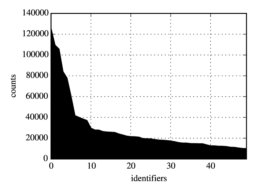
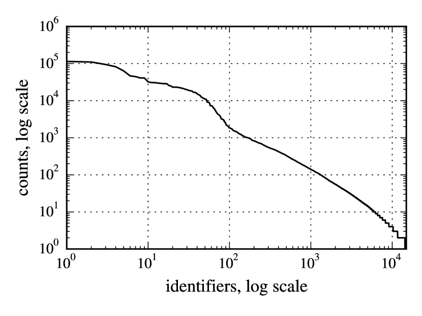
The distribution of counts for identifiers inside the documents also appears to follow a long tail power law distribution: there are few articles that contain many identifiers, while most of the articles do not (see fig. 4(a)). The biggest article (‘‘Euclidean algorithm’’) has 22 766 identifiers, and the second largest (‘‘Lambda lifting’’) has only 6 500 identifiers. The mean number of identifiers per document is 33. The distribution of the number of distinct identifiers per document is less skewed (see fig. 4(b)). The largest number of distinct identifiers is 287 (in the article ‘‘Hooke’s law’’), and it is followed by 194 (in ‘‘Dimensionless quantity’’). The median number of identifiers per document is 10.

(a) Identifier frequencies per document for first 80 most largest documents

(b) No. of distinct identifiers per document for first 80 most largest documents

(c) Definitions per document

Figure 4: Frequencies per documents

For 12 771 identifiers the algorithm extracted 115 300 definitions, and the number of found definitions follows a long tail distribution as well (see fig. 4(c)), with the median number of definitions per page being 4.

ID	Definition	Count	Definition Rus	Count
$t$	time	1086	время	130
$m$	mass	424	масса	103
$\theta$	angle	421
$T$	temperature	400	температура	69
$r$	radius	395
$v$	velocity	292	скорость	50
$\rho$	density	290	плотность	57
$G$	group	287	группа	87
$V$	volume	284
$\lambda$	wavelength	263
$R$	radius	257	радиус	38
$n$	degree	233
$r$	distance	220
$c$	speed of light	219	скорость свет	89
$L$	length	216
$n$	length	189
$n$	order	188
$n$	dimension	185
$n$	size	178
$M$	mass	171
$d$	distance	163
$X$	topological space	159	топ. пространство	46

Table 1: Most frequent relations from the English Wikipedia and corresponding relations from the Russian Wikipedia.

Table 1 shows the list of the most common identifier-definition relations extracted from the English Wikipedia.

In the Russian Wikipedia only 5 300 articles contain enough identifiers, and the remaining 9 500 are discarded.

The identifiers and definitions extracted from the Russian version of Wikipedia exhibit the similar properties. The most frequently occurring identifier is ‘‘$x$’’ with 13 248 occurrences, but the median frequency of an identifer is only 3 times. The article with the largest number of identifiers is ‘‘Уравнения Максвелла’’ (‘‘Maxwell’s equations’’), which contains 1 831 identifiers, while the median number of identifiers is just 3; the article with the largest number of distinct identifiers is also ‘‘Уравнения Максвелла’’ with 112 unique identifiers, and the median number of distinct identifiers in the data set is 5. Finally, the largest number of extracted definitions is 44 (again, for ‘‘Уравнения Максвелла’’) with 2 being the median number of definitions per page.

We can compare the most frequent identifier-definition relations extracted from the Russian Wikipedia (see table 1): some of the top relations appear in both datasets. Other frequent identifier-definition relations extracted from the Russian Wikipedia include:

• $f$: ‘‘функция’’ (‘‘function’’) (215)

• $X$: ‘‘множество’’ (‘‘set’’) (113)

• $h$: ‘‘постоянный планка’’ (‘‘Planck constant’’) (68)

• $M$: ‘‘многообразие’’ (‘‘manifold’’) (53)

• $K$: ‘‘поль’’ (‘‘field’’) (53)

• $X$: ‘‘пространство’’ (‘‘space’’) (50)

• $G$: ‘‘граф’’ (‘‘graph’’) (44)

• $R$: ‘‘радиус’’ (‘‘radius’’) (38)

• $R$: ‘‘кольцо’’ (‘‘ring’’) (36)

• $G$: ‘‘гравитационный постоянный’’ (‘‘gravitational constant’’) (34)

• $E$: ‘‘энергия’’ (‘‘energy’’) (34)

• $m$: ‘‘модуль’’ (‘‘modulo’’) (33)

• $S$: ‘‘площадь’’ (‘‘area’’) (32)

• $k$: ‘‘постоянный больцмана’’ (‘‘Boltzmann constant’’) (30)

4.3 Document Clustering

At the document clustering stage we want to find cluster of documents that are good namespace candidates.

Before we can do this, we need to vectorize our dataset: i.e., build the identifier space (see section 3.4) and represent each document in this space.

There are three choices for dimensions of the identifier space:

• identifiers alone,

• ‘‘weak’’ identifier-definition association,

• ‘‘strong’’ association: using identifier-definition pairs.

In the first case we are only interested in identifier information and discard the definitions altogether.

In the second and third cases we keep the definitions and use them to index the dimensions of the identifier space. But there is some variability in the definitions: for example, the same identifier ‘‘$\sigma$’’ in one document can be assigned to ‘‘Cauchy stress tensor’’ and in other it can be assigned to ‘‘stress tensor’’, which are almost the same thing. To reduce this variability we perform some preprocessing: we tokenize the definitions and use individual tokens to index dimensions of the space. For example, suppose we have two pairs ($\sigma$, ‘‘Cauchy stress tensor’’) and ($\sigma$, ‘‘stress tensor’’). In the ‘‘weak’’ association case we have will dimensions $(\sigma,\text{Cauchy},\text{stress},\text{tensor})$, while for the ‘‘strong’’ association case we will have $(\sigma\text{\_Cauchy},\sigma\text{\_stress},\sigma\text{\_tensor})$.

Additionally, the effect of variability can be decreased further by applying a stemming technique for each definition token. In this work we use Snowball stemmer for English [56] implemented in NLTK [57]: a Python library for Natural Language Processing. For Russian we use Pymorphy2 [55].

Using TfidfVectorizer from scikit-learn [58] we vectorize each document. The experiments are performed with $(\log\text{TF})\times\text{IDF}$ weighting, and therefore we use use_idf=False, sublinear_tf=True parameters for the vectorizer. Additionally, we use min_df=2 to discard identifiers that occurs only once.

The output is a document-identifier matrix (analogous to ‘‘document-term’’): documents are rows and identifiers/definitions are columns. The output of TfidfVectorizer is row-normalized, i.e. all rows have unit length.

Once we the documents are vectorized, we can apply clustering techniques to them. We use $K$-Means (see section 2.6.2) implemented as a class KMeans in scikit-learn and Mini-Batch $K$-Means (class MiniBatchKMeans) [58]. Note that if rows are unit-normalized, then running $K$-Means with Euclidean distance is equivalent to cosine distance (see section 2.5.3).

DBSCAN and SNN Clustering (see section 2.6.3) algorithms were implemented manually: available DBSCAN implementations usually employ a distance measure rather than a similarity measure. The similarity matrix created by similarity measures are typically very sparse, usually because only a small fraction of the documents are similar to some given document. Similarity measures can be converted to distance measures, but in this case the matrix will no longer be sparse, and we would like to avoid that. Additionally, available implementations are usually general purpose implementations and do not take advantage of the structure of the data: in text-like data clustering algorithms can be sped up significantly by using an inverted index.

Dimensionality reduction techniques are also important: they not only reduce the dimensionality, but also help reveal the latent structure of data. In this work we use Latent Semantic Analysis (LSA) (section 2.7) which is implemented using randomized Singular Value Decomposition (SVD) [59], The implementation of randomized SVD is taken from scikit-learn [58] – method randomized_svd. Non-negative Matrix Factorization is an alternative technique for dimensionality reduction (section 2.7). Its implementation is also taken from scikit-learn [58], class NMF.

To assess the quality of produced clusters we use wikipedia categories. It is quite difficult to extract category information from raw wikipedia text, therefore we use DBPedia [60] for that: it provides machine-readable information about categories for each wikipedia article. Additionally, categories in wikipedia form a hierarchy, and this hierarchy is available as a SKOS ontology.

Unfortunately, there is no information about articles from the Russian Wikipedia on DBPedia. However the number of documents is not very large, and therefore this information can be retrieved via MediaWiki API individually for each document. This information can be retrieved in chunks for a group of several documents at once, and therefore it is quite fast.

4.4 Building Namespaces

Once a cluster analysis algorithm assigns documents in our collection to some clusters, we need to find namespaces among these clusters. We assume that some clusters are namespace-defining: they are not only homogenous in the cluster analysis sense (for example, in case of $K$-Means it means that within-cluster sum of squares is minimal), but also ‘‘pure’’: they are about the same topic.

A cluster is pure if all documents belong to the same category. Using categories information we can find the most frequent category of the cluster, and then we can define purity of a cluster $C$ as

$$\operatorname{purity}(C)=\cfrac{\max_{i}\operatorname{count}(c_{i})}{|C|},$$

where $c_{i}$’s are cluster categories. Thus we can select all clusters with purity above some pre-defined threshold and refer to them as namespace-defining clusters.

Then we convert these clusters into namespaces by collecting all the identifiers and their definitions in the documents of each cluster. To do this, we first collect all the identifier-definition pairs, and then group them by identifier. When extracting, each definition candidate is scored, and this score is used to determine, which definition an identifier will be assigned in the namespace.

For example, consider three documents with the following extracted relations:

• Document A:

  • $n$: (predictions, 0.95), (size, 0.92), (random sample, 0.82), (population, 0.82)

  • $\theta$: (estimator, 0.98), (unknown parameter, 0.98), (unknown parameter, 0.94)

  • $\mu$: (true mean, 0.96), (population, 0.89)

  • $\mu_{4}$: (central moment, 0.83)

  • $\sigma$: (population variance, 0.86), (square error, 0.83), (estimators, 0.82)

• Document B:

  • $P_{\theta}$: (family, 0.87)

  • $X$: (measurable space, 0.95), (Poisson, 0.82)

  • $\theta$: (sufficient statistic, 0.93)

  • $\mu$: (mean, 0.99), (variance, 0.95), (random variables, 0.89), (normal, 0.83)

  • $\sigma$: (variance, 0.99), (mean, 0.83)

• Document C:

  • $n$: (tickets, 0.96), (maximum-likelihood estimator, 0.89)

  • $x$: (data, 0.99), (observations, 0.93)

  • $\theta$: (statistic, 0.95), (estimator, 0.93), (estimator, 0.93), (rise, 0.91), (statistical model, 0.85), (fixed constant, 0.82)

  • $\mu$: (expectation, 0.96), (variance, 0.93), (population, 0.89)

  • $\sigma$: (variance, 0.94), (population variance, 0.91), (estimator, 0.87)

We take all these relations, and combine together. If an identifer has two or more definitions that are exactly the same, them we merge them into one and its score is the sum of scores:

• $P_{\theta}$: (family, 0.87)

• $X$: (measurable space, 0.95), (Poisson, 0.82)

• $n$: (tickets, 0.96), (predictions, 0.95), (size, 0.92), (maximum-likelihood estimator, 0.89), (random sample, 0.82), (population, 0.82)

• $x$: (data, 0.99), (observations, 0.93)

• $\theta$: (estimator, 0.98+0.93+0.93), (unknown parameter, 0.98+0.94), (statistic, 0.95), (sufficient statistic, 0.93), (rise, 0.91), (statistical model, 0.85), (fixed constant, 0.82)

• $\mu$: (random variables, 0.89+0.89+0.89), (variance, 0.95+0.93), (mean, 0.99), (true mean, 0.96), (expectation, 0.96), (normal, 0.83)

• $\mu_{4}$: (central moment, 0.83)

• $\sigma$: (variance, 0.99+0.94), (population variance, 0.91+0.86), (estimator, 0.87), (square error, 0.83), (mean, 0.83), (estimators, 0.82)

There is some lexical variance in the definitions. For example, ‘‘variance’’ and ‘‘population variance’’ or ‘‘mean’’ and ‘‘true mean’’ are very related definitions, and it makes sense to group them together to form one definition. It can be done by fuzzy string matching (or approximate matching) [61]. To implement it, we use a Python library FuzzyWuzzy [62], and using fuzzy matching we group related identifiers and then sum over their scores.

Then we have the following:

• $P_{\theta}$: (family, 0.87)

• $X$: (measurable space, 0.95), (Poisson, 0.82)

• $n$: (tickets, 0.96), (predictions, 0.95), (size, 0.92), (maximum-likelihood estimator, 0.89), (random sample, 0.82), (population, 0.82)

• $x$: (data, 0.99), (observations, 0.93)

• $\theta$: (estimator, 2.84), (unknown parameter, 1.92), ({statistic, sufficient statistic}, 1.88), (rise, 0.91), (statistical model, 0.85), (fixed constant, 0.82)

• $\mu$: (random variables, 2.67), ({mean, true mean}, 1.95), (variance, 1.88), (expectation, 0.96), (normal, 0.83)

• $\mu_{4}$: (central moment, 0.83)

• $\sigma$: ({variance, population variance}, 3.7), ({estimator, estimators}, 1.69), (square error, 0.83), (mean, 0.83)

In a namespace an identifier can have at most one definition, and therefore the next step is selecting the definition with the highest score. This gives us the following namespace:

• ($P_{\theta}$, family, 0.87)

• ($X$, measurable space, 0.95)

• ($n$, tickets, 0.96)

• ($x$, data, 0.99)

• ($\theta$, estimator, 2.84)

• ($\mu$, random variables, 2.67)

• ($\mu_{4}$, central moment, 0.83)

• ($\sigma$: variance, 3.7)

Intuitively, the more a relation occurs, the higher the score, and it gives us more confidence that the definition is indeed correct.

Figure 5: Non-linear transformation of scores with $\tanh$ function.

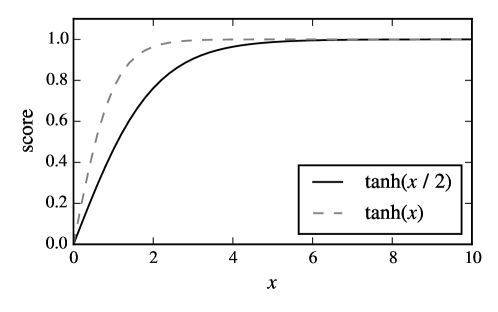
However, it is more convenient to compare scores when they are on the $[0,1]$ scale, and therefore we may apply additional transformation to convert the scores. Hyperbolic tangent function is a good choice for such transformation: it is near zero for small values and it never exceeds one (see fig. 5) But it is quite steep and converges to 1 rather quickly: for a relation with score of 3 it would produce a score of 0.99, which is quite high. Instead, we can use a less steep $\tanh(x/2)$ (see fig. 5): for 3, $\tanh(3/2)$ produces a score of 0.90, which is better.

Because the hyperbolic tangent is a monotonously increasing function, larger values of the original score correspond to larger values of the transformed score, and therefore we still can use the output of $\tanh(x/2)$ to rank the relations.

Thus, after applying this transformation, we obtain the following namespace:

• ($P_{\theta}$, family, 0.41)

• ($X$, measurable space, 0.44)

• ($n$, tickets, 0.45)

• ($x$, data, 0.46)

• ($\theta$, estimator, 0.89)

• ($\mu$, random variables, 0.87)

• ($\mu_{4}$, central moment, 0.39)

• ($\sigma$: variance, 0.95)

The name for this namespace is selected as the category that the majority of the documents in the namespace-defining cluster share.

5 Evaluation

In this chapter we describe the experimental setup and the obtained results.

The following software is used for the experiments: Apache Flink 0.8.1 [47] numpy 1.9.2 [63], scipy 0.15.1 [64], scikit-learn 0.16.1 [58] and IPython notebook 3.1.0. The experiments are run on a 64-bit Windows machine with two CPUs of 2.10 GHz and 8 GB of RAM.

First, section 5.1 verifies that the namespace discovery is possible by applying the proposed technique to Java source code. Next, section 5.2 describes parameter tuning: there are many possible choices of parameters, and we find the best. Once the best algorithm and its parameters are selected, we analyze the obtained results in section 5.3. Next, we describe how the discovered clusters can be mapped to a hierarchy in section 5.4, and finish by summarizing our findings in section 5.5.

5.1 Java Language Processing

There is no ‘‘gold standard’’ data set for the namespace discovery problem because this problem has not been studied, and it is hard to verify if our approach works or not.

Previously we have illustrated the idea of identifier namespaces by comparing it with namespaces in Computer Science, and it allowed us to develop an intuition behind the namespaces in mathematics and also propose a method to discover them: we motivated the assumption that there exist ‘‘namespace defining’’ groups of documents by arguing that these groups also exist in programming languages.

Therefore we try to use source code as a dataset, and see whether our method is able to recover namespace information or not.

If a programming language is statically typed, like Java or Pascal, usually it is possible to know the type of a variable from the declaration of this variable. Therefore we can see variable names as ‘‘identifiers’’ and variable types as ‘‘definitions’’. Clearly, there is a difference between variable types and identifier definitions, but we believe that this comparison is valid because the type carries additional semantic information about the variable and in what context it can be used – like the definition of an identifier.

The information about variables and their types can be extracted from a source code repository, and each source file can be processed to obtain its Abstract Syntax Tree (AST). By processing the ASTs, we can extract the variable declaration information. Thus, each source file can be seen as a document, which is represented by all its variable declarations.

In this work we process Java source code, and for parsing it and building ASTs we use a library JavaParser [65]. The Java programming language was chosen because it requires the programmer to always specify the type information when declaring a variable. It is different for other languages when the type information is usually inferred by the compilers at compilation time.

In Java a variable can be declared in three places: as an inner class variable (or a ‘‘field’’), as a method (constructor) parameter or as a local variable inside a method or a constructor. We need to process all three types of variable declarations and then apply additional preprocessing, such as converting the name of the type from short to fully qualified using the information from the import statements. For example, String is converted to java.lang.String and List<Integer> to java.util.List<Integer>, but primitive types like byte or int are left unchanged.

Consider an example in the listing 1. There is a class variable threshold, a method parameter in and two local variables word and posTag. The following relations will be extracted from this class: (‘‘threshold’’, double), (‘‘in’’, domain.Word), (‘‘word’’, java.lang.String), (‘‘posTag’’, java.lang.String). Since all primitives and classes from packages that start with java are discarded, at the end the class WordProcesser is represented with only one relation (‘‘in’’, domain.Word).

Listing 1: A Java class

⬇

package process;

import domain.Word;

public class WordProcesser {

private double threshold;

public boolean isGood(Word in) {

String word = in.getWord();

String posTag = in.getPosTag();

return isWordGood(word) && isPosTagGood(posTag);

}

// ...

}

In the experiments we applied this source code analysis to the source code of Apache Mahout 0.10 [66], which is an open-source library for scalable Machine Learning and Data Mining. As on , this dataset consists of 1 560 java classes with 45 878 variable declarations. After discarding declarations from the standard Java API, primitives and types with generic parameters, only 15 869 declarations were retained.

The following is top-15 variable/type declarations extracted from the Mahout source code:

• ‘‘conf’’, org.apache.hadoop.conf.Configuration (491 times)

• ‘‘v’’, org.apache.mahout.math.Vector (224 times)

• ‘‘dataModel’’, org.apache.mahout.cf.taste.model.DataModel (207 times)

• ‘‘fs’’, org.apache.hadoop.fs.FileSystem (207 times)

• ‘‘log’’, org.slf4j.Logger (171 times)

• ‘‘output’’, org.apache.hadoop.fs.Path (152 times)

• ‘‘vector’’, org.apache.mahout.math.Vector (145 times)

• ‘‘x’’, org.apache.mahout.math.Vector (120 times)

• ‘‘path’’, org.apache.hadoop.fs.Path (113 times)

• ‘‘measure’’, org.apache.mahout.common.distance.DistanceMeasure (102 times)

• ‘‘input’’, org.apache.hadoop.fs.Path (101 times)

• ‘‘y’’, org.apache.mahout.math.Vector (87 times)

• ‘‘comp’’, org.apache.mahout.math.function.IntComparator (74 times)

• ‘‘job’’, org.apache.hadoop.mapreduce.Job (71 times)

• ‘‘m’’, org.apache.mahout.math.Matrix (70 times)

We use the ‘‘soft’’ association method to incorporate ‘‘definition’’ (i.e. types), and considering each source code file as a document, we build an identifier-document matrix of dimensionality $1436\times 1560$. Only identifiers that occur at least twice are used to build the matrix.

To discover namespace-defining cluster, we use LSA with SVD and MiniBatch $K$-Means. For weight assignment, we try two weighting systems: usual TF component and sublinear TF. The best performance is achieved with the rank $k=200$ of SVD and number of clusters $K=200$ using sublinear weighting (see fig. 6).

(a) Usual TF $\times$ IDF weighting

(b) $(\log\text{TF})\times\text{IDF}$ weighting

Figure 6: The performance MiniBatch $K$-Means on the Mahout dataset.

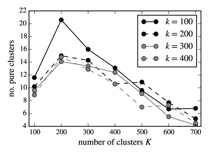
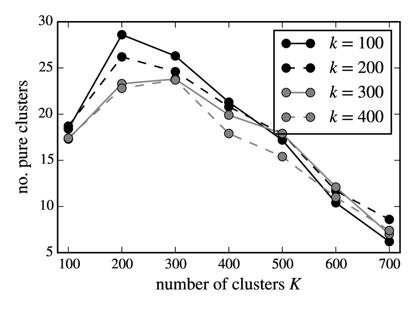
With these parameters the best result is 33 clusters (see table 2(a)). One of such clusters is a cluster about SVD: there are 5 classes from the svd package (Factorization, FilePersistenceStrategy, NoPersistenceStrategy, PersistenceStrategy, FilePersistenceStrategyTest) and one from
kddcup.track1.svd package (Track1SVDRunner). Although this cluster is not 100% pure, in the sense that not all of these classes belong to the same package, these classes are clearly related: they are all about SVD. The top dimensions with the most influence in this cluster are svd.Factorization and factorization.

Another interesting namespace is the distance namespace, with classes mostly from common.distance (see table 2(b)). What is interesting, there are mostly tests in this cluster, but because they use classes that they test, they roughly can be seen as documents that refer to some concepts defined outside of the cluster (see table 2(c)).

Size	Namespace	Purity
16	org.apache.mahout.h2obindings.ops	0.88
12	org.apache.mahout.math.map	0.92
11	org.apache.mahout.text	0.91
10	org.apache.mahout.vectorizer.collocations.llr	1.00
10	org.apache.mahout.classifier.sequencelearning.hmm	1.00
10	org.apache.mahout.math.list	1.00
9	org.apache.mahout.math.map	0.89
9	org.apache.mahout.cf.taste.hadoop.item	1.00
8	org.apache.mahout.cf.taste.hadoop.als	1.00
8	org.apache.mahout.classifier.sgd	0.88

(a) Top namespace-defining clusters discovered from Mahout.

Class name
org.apache.mahout.math.neighborhood.UpdatableSearcher
org.apache.mahout.common.distance.CosineDistanceMeasureTest
org.apache.mahout.common.distance.DefaultDistanceMeasureTest
org.apache.mahout.common.distance.DefaultWeightedDistanceMeasureTest
org.apache.mahout.common.distance.TestChebyshevMeasure
org.apache.mahout.common.distance.TestMinkowskiMeasure

(b) A namespace-defining cluster about Distances.

ID	Class
chebyshevDistanceMeasure	org.apache.mahout.common.distance.DistanceMeasure
distanceMeasure	org.apache.mahout.common.distance.DistanceMeasure
euclideanDistanceMeasure	org.apache.mahout.common.distance.DistanceMeasure
manhattanDistanceMeasure	org.apache.mahout.common.distance.DistanceMeasure
minkowskiDistanceMeasure	org.apache.mahout.common.distance.DistanceMeasure
v	org.apache.mahout.math.Vector
vector	org.apache.mahout.math.Vector

(c) Definitions in the v namespace.

Table 2: Namespaces extracted from Apache Mahout source code.

We are able to discover 33 namespaces using the Mahout source code as a dataset. There are 150 packages in total. This means that using only identifier information it is enough to recover namespace information at least partially (in our case, we can recover 22% of the namespaces).

Therefore, in principle, the approach works and it can be used to discover namespaces in mathematics.

5.2 Parameter Tuning

There are many different clustering algorithms, each with its own set of parameter. In this section we describe how we find the settings that find the best namespaces.

The following things can be changed:

• Ways to incorporate definition information (no definitions, soft association, hard association);

• Weighting schemes for the identifier-document matrix $D$: TF, sublinear TF, TF-IDF;

• There are different clustering algorithms: agglomerative clustering, DBSCAN, SNN clustering, $K$-Means, and each algorithm has its own set of parameters;

• Dimensionality of $D$ can be reduced via SVD or NMF, parameter $k$ controls the rank of output.

To find the best parameters set we use the grid search approach: we try different combinations of parameters and keep track on the number of pure clusters and the purity.

The overall purity of cluster assignment is calculated as a weighed sum of individual cluster purities, where the weight is chosen proportionally to the size of a cluster.

(a) Number of clusters $K$ vs overall purity of clustering: the purity increases linearly with $K$ ($R^{2}=0.99$).

(b) Number of clusters $K$ vs the number of pure clusters: it grows initially, but after $K\approx 8\,000$ starts to decrease.

Figure 7: Purity and number of pure clusters as measures of algorithm performance.

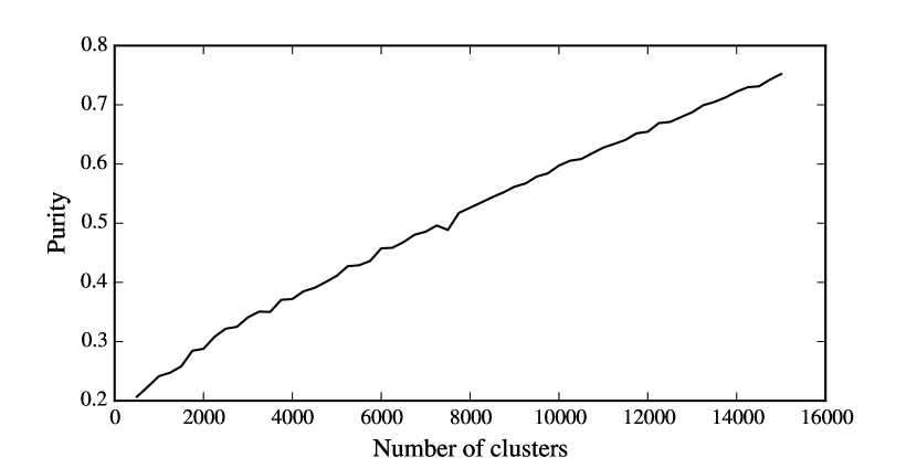
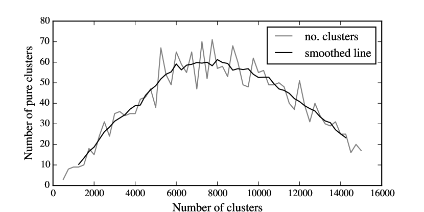
However it is not enough just to find the most pure cluster assignment: because as the number of clusters increases the overall purity also grows. Thus we can also optimize for the number of clusters with purity $p$ of size at least $n$. When the number of clusters increase, the purity always grows (see fig. 7(a)), but at some point the number of pure clusters will start decreasing (see fig. 7(b)).

5.2.1 Baseline

We compare the performance of clustering algorithms against a random categorizer. The simplest version of such a categorizer is the random cluster assignment categorizer, which assigns each document to some random cluster. In this case, we constrain the categorizer to include 3 documents in each cluster, and once a document belongs to some cluster, it cannot be re-assigned. It is done by first creating a vector of assignments and shuffling it.

Then we record how many pure clusters (at least 80% pure) are in the cluster assignment.

Figure 8: Distribution of the number of pure clusters across 200 trials.

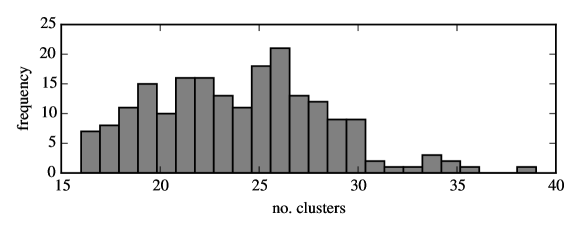
To establish the baseline, we repeated this experiment for 200 times (see fig. 8), and the maximal achieved value is 39 pure clusters, while the mean value is 23.85.

5.2.2 Only Identifiers

The first way of building the identifier space is to use only identifiers andW not use definitions at all. If we do this, the identifier-document matrix is $6075\times 22512$ (we keep only identifiers that occur at least twice), and it contains 302  541 records, so the density of this matrix is just 0.002.

First, we try to apply agglomerative clustering, then DBSCAN with SNN similarity based on Jaccard coefficient and cosine similarity, then we do $K$-Means and finally we apply LSA using SVD and NMF and apply $K$-Means on the reduced space.

Figure 9: Runtime of agglomerative clustering is quadratic with the number of documents in the collection ($R^{2}=0.99$).

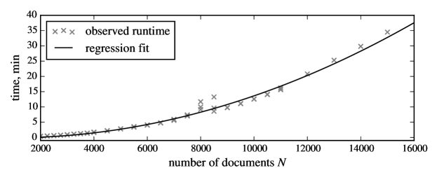
Agglomerative clustering algorithms are quite fast for small datasets, but they become more computationally expensive as the dataset size grows. We run a series of experiments on subsamples of our dataset and we can observe that the run time is quadratic with the number of documents to cluster (see fig. 9). The polynomial regression model that we built predicts that it should process the entire dataset of 22 512 documents in 90 minutes, but it was not able to finish in several hours, so we stopped the computation. Additionally, the implementation we use from scikit-learn requires a dense matrix. But when densified, the identifier-document matrix occupies a lot of space: if each element of the matrix is represented with a double precision number, then this matrix occupies 1.01 GB of RAM in total. While it is small enough to fit into memory, matrices of larger dimensionality might not. Therefore, we exclude these clustering algorithms from further analysis.

(a) Number of clusters when 10 nearest neighbors are considered

(b) Performance of selected $\varepsilon$ with 10 nearest neighbors

(c) Number of clusters when 15 nearest neighbors are considered

(d) Performance of selected $\varepsilon$ with 15 nearest neighbors

Figure 10: Effect of parameters $\varepsilon$, MinPts and number of nearest neighbors on performance of SNN DBSCAN when Jaccard coefficient is used.

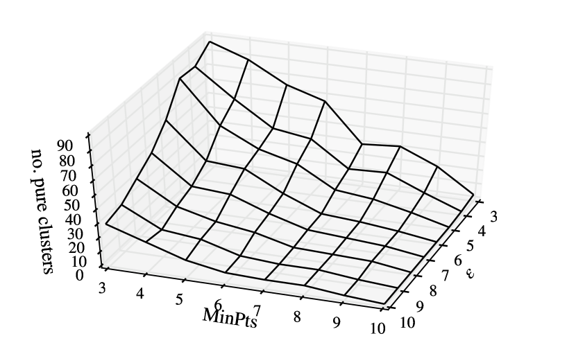
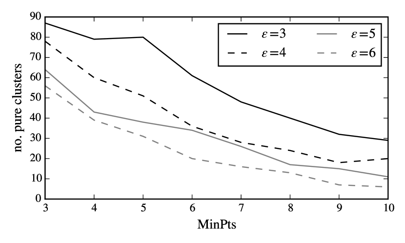
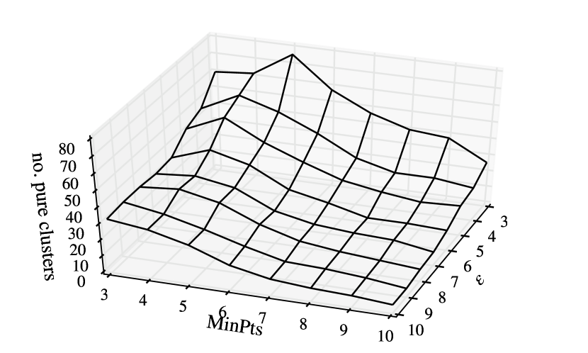
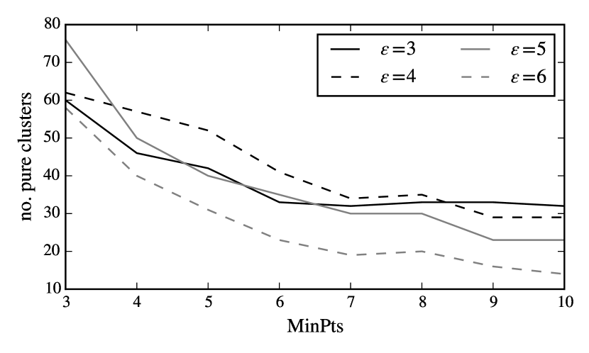
The second method is DBSCAN with SNN Similarity. To compute SSN similarity we need to use some other base similarity measure. We start with Jaccard coefficient, and use a binarized identifier-document matrix: a matrix with only ones and zeros. For example, the closest article to ‘‘Linear Regression’’ is ‘‘Linear predictor function’’ with Jaccard coefficient of 0.59 and ‘‘Low-rank approximation’’ is the closest to ‘‘Singular value decomposition’’ with coefficient of 0.25. With Jaccard, we were able to discover 87 clusters, which is two times better than the baseline (see fig. 10) and the best parameters are 10 nearest neighbors, $\varepsilon=3$ and MinPts $=4$ (see fig. 10(b)).

Then we run the same algorithm, but with cosine similarity, using an identifier-document matrix with $(\log\text{TF})\times\text{IDF}$ weights, and calculate pair-wise similarity between each document. For example, let us take an article ‘‘Linear regression’’ and calculate the cosine with the rest of the corpus. The closest document is ‘‘Linear predictor function’’. They have 23 identifiers in common, and they indeed look related. However cosine is not always giving the best closets neighbors. For example, the nearest neighbor of ‘‘Singular value decomposition’’ is ‘‘Rule of Sarrus’’, and although their cosine score is 0.92, they have only 3 identifiers in common.

(a) Number of clusters when 10 nearest neighbors are considered

(b) Performance of selected $\varepsilon$ with 10 nearest neighbors

(c) Number of clusters when 15 nearest neighbors are considered

(d) Performance of selected $\varepsilon$ with 15 nearest neighbors

Figure 11: Effect of parameters $\varepsilon$, MinPts and number of nearest neighbors on performance of SNN DBSCAN when cosine is used.

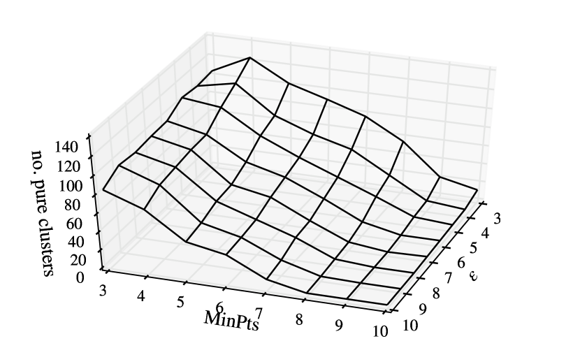
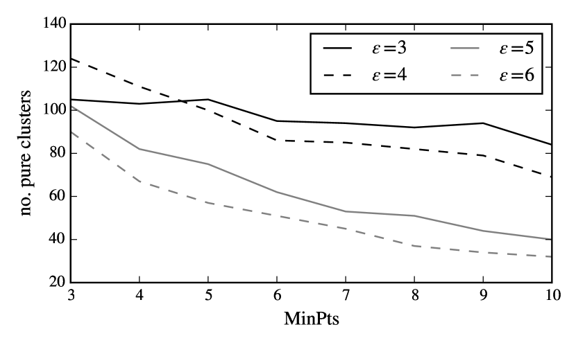
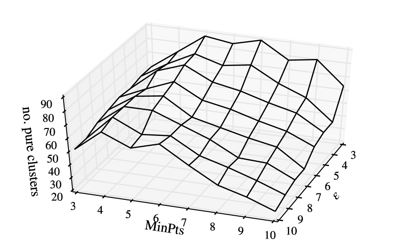
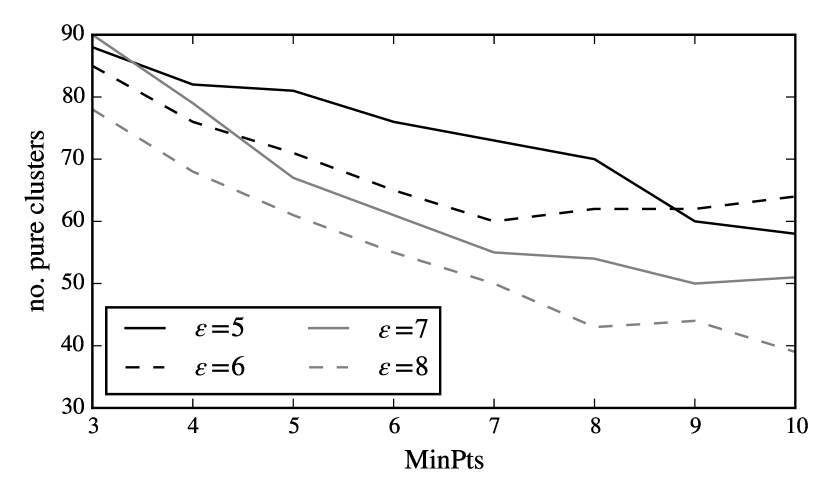
With cosine as the base similarity function for SNN DBSCAN we were able to discover 124 namespace-defining clusters (see fig. 11), which is significantly better than the baseline. The best parameters are 10 nearest neighbors and $\varepsilon=4$, MinPts $=3$ (see fig. 11(b)).

(a) $K$ in $K$-Means vs time in minutes ($R^{2}=0.99$).

(b) $K$ in MiniBatch $K$-Means vs time in seconds ($R^{2}=0.97$).

Figure 12: Runtime of $K$-Means and MiniBatch $K$-Means

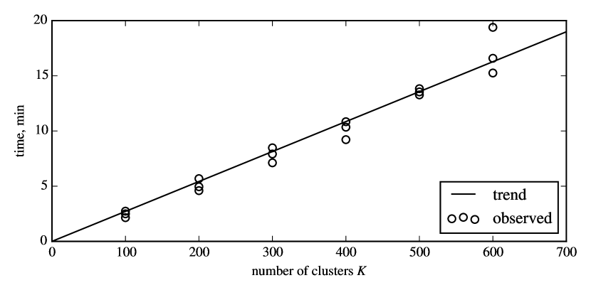
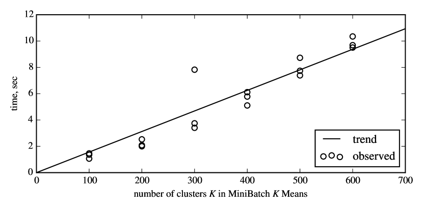
Next, we apply $K$-Means. We observe that increasing $K$ leads to linear increase in time (see fig. 12(a)), which means that for bigger values of $K$, it takes longer, so it is not feasible to run: for example, we estimate the runtime of $K$-Means with $K=10\,000$ to be about 4.5 hours. As MiniBatch $K$-Means is expected to be significantly faster than usual $K$-Means, we use it as well. Although we observe that the run time of MiniBatch $K$-Means also increases linearly with $K$ (see fig. 12(b)), it indeed runs considerably faster. For example, MiniBatch $K$-Means takes 15 seconds with $K=700$ while usual $K$-Means takes about 15 minutes (see fig. 12(a) and fig. 12(b)).

(a) Purity vs number of clusters $K$ in $K$-Means and MiniBatch $K$-Means

(b) Number of pure clusters vs $K$ in $K$-Means and MiniBatch $K$-Means

(c) Number of pure clusters vs $K$ in MiniBatch $K$-Means for larger $K$

Figure 13: Effect of $K$ on performance in $K$-Means

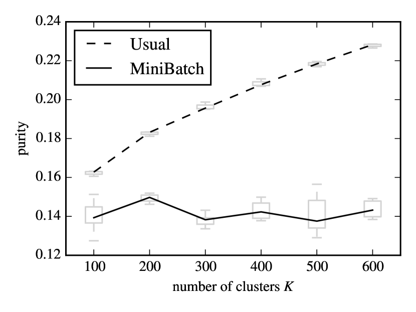
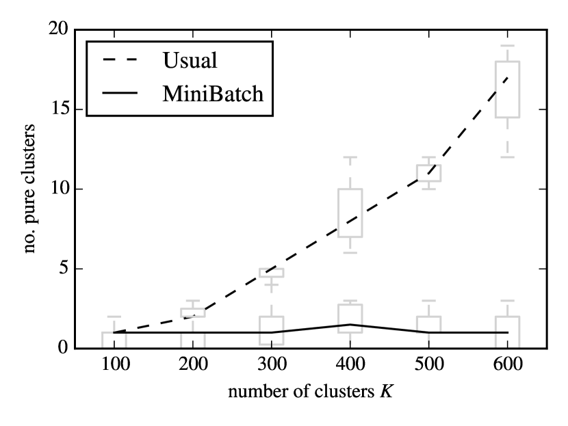
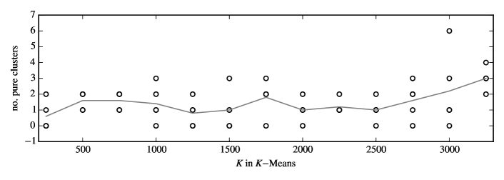
Usual $K$-Means with small $K$ does not find many pure clusters, and MiniBatch $K$-Means does even worse: independently of the choice of $K$, the number of pure clusters and purity does not change significantly (see fig. 13(a) and fig. 13(b)). This is also true for larger values of $K$ (see fig. 13(c)).

The best result was found by usual $K$-Means with $K=600$: it was able to discover 19 clusters with purity at least 0.8 (note that this is worse than the baseline of 39 pure clusters).

Next, we use Latent Semantic Analysis with SVD to reduce the dimensionality of the identifier-document matrix $D$, and then apply $K$-Means on the reduced space. As discussed in the LSA section (see section 2.7), it should reveal the latent structure of data. Hence, we expect that it should improve the results achieved by usual $K$-Means.

Figure 14: Effect of $k$ in $k$-rank-reduced randomized SVD on the runtime in seconds.

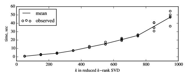
Randomized SVD is very fast, but the runtime does not grow linearly with $k$, it looks quadratic (see fig. 14). However, the typical values of $k$ for SVD used in latent semantic analysis is 150-250 [22] [39], therefore the run time is not prohibitive, and we do not need to rut it with very large $k$.

(a) Purity vs number of clusters $K$ in $K$-Means and MiniBatch $K$-Means.

(b) Number of pure clusters vs $K$ in $K$-Means and MiniBatch $K$-Means.

Figure 15: The performance of $K$-Means and MiniBatch $K$-Means on the reduced document space with $k=150$.

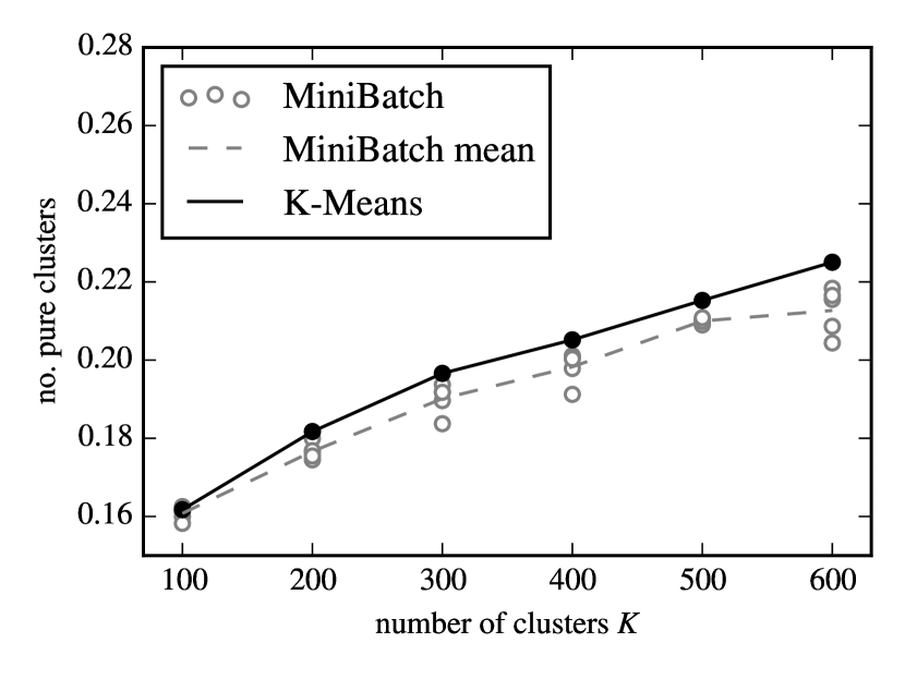
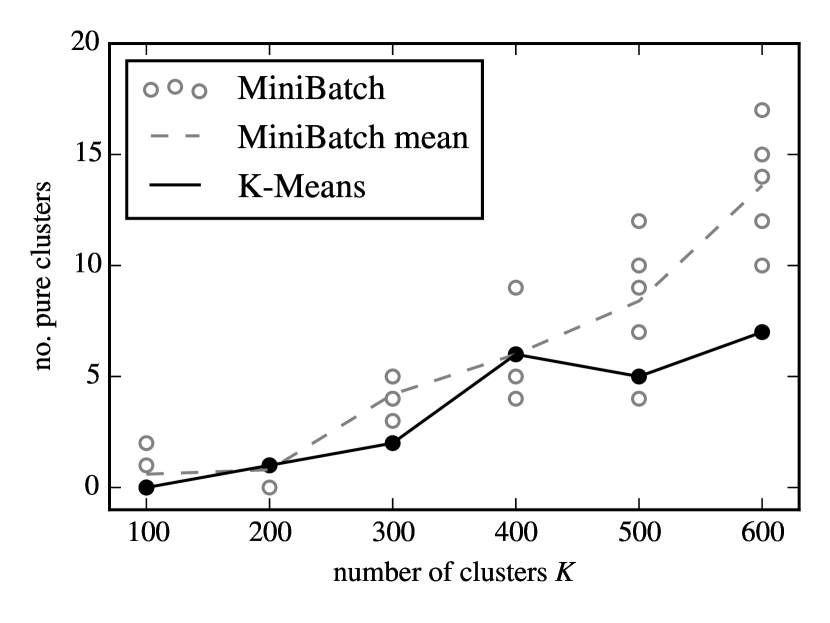
When the dimensionality is reduced, the performance of $K$-Means and MiniBatch $K$-Means is similar (see fig. 15(a)), but with MiniBatch $K$-Means we were able to discover more interesting pure clusters (see fig. 15(b)). The reason for this may be the fact that in the reduced space there is less noise and both methods find equally good clusters, but because MiniBatch $K$-Means works faster, we are able to run it multiple times thus increasing its chances to find a good local optimum where there are many pure document clusters. Note that the obtained result is below the baseline.

We can observe that as $K$ increases, the number of interesting clusters increases (see fig. 15(b)). Therefore, we try a wide range of larger $K$ for different $k\in\{150,250,350,500\}$. The performance in terms of discovered pure clusters does not depend much on the rank $k$ of the reduced space (see fig. 16). In fact, it is very hard to distinguish different lines because they are quite perplexed. The maximum for is achieved at $K\approx 10\,000$ for all $k$.

Figure 16: Number of discovered pure clusters in $K$-Means for different number of clusters $K$ and rank $k$.

Figure 17: Runtime of NMF for different $k$.

Figure 18: Number of discovered pure clusters in $K$-Means and NMF for different number of clusters $K$ and rank $k$.

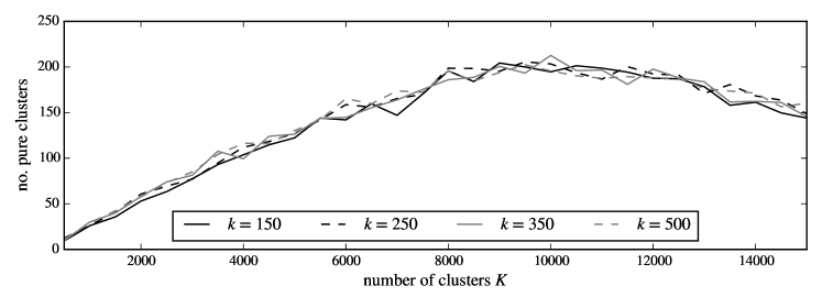
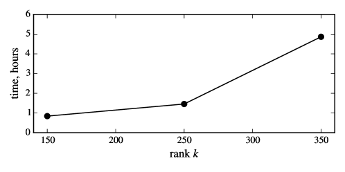
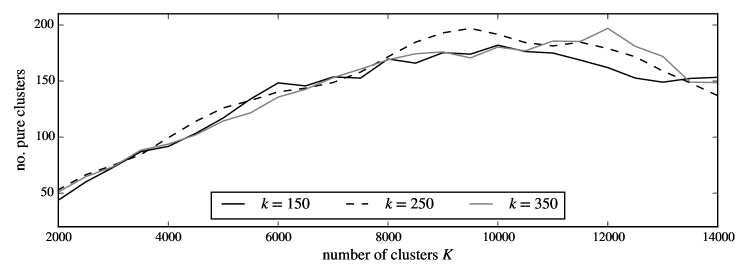
We also can apply Non-Negative Matrix Factorization for LSA. NMF takes significantly more time than randomized SVD (see fig. 17). In addition, although the runtime should be $O(nk)$ [42], we do not observe that it grows linearly with $k$. On the contrary, it appears that there is rather quadratic relationship. We expected that the results produced by NMF will be better than SVD because of non-negativity of produced results, but the performance is quite similar (see fig. 18). For NMF, however, it is easier to see the difference in performance when different rank $k$ is used, and the curves are not as perplexed as for SVD. We see that $k=250$ does better on $K=[8000;12000]$ than $k=150$ and $k=350$. For example, $K$-Means with $K=9500$ and $k=250$ discovered a clustering with 200 namespace-defining clusters.

We can also observe that generally clustering works better on reduced spaces.

Figure 19: The effect of using different weighting systems on $K$-Means with SVD.

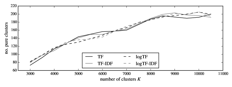
In the experiments above we used the $(\log\text{TF})\times\text{IDF}$ weighting scheme. Let us compare the effect of different weighting on the resulting clusters. To do that, we apply SVD with $k=150$ and run MiniBatch $K$-Means for a set of smaller $K$’s because it is computationally faster. We can observe that performance of $K$-Means does not depend significantly on the weighting system when no definitions are used (see fig. 19).

5.2.3 Weak Association

The identifier-document matrix has the dimensionality $10419\times 22512$, and there are 485 337 elements in the matrix, so the density is about 0.002.

(a) Number of clusters when 10 nearest neighbors are considered

(b) Performance of selected $\varepsilon$ with 10 nearest neighbors

(c) Number of clusters when 15 nearest neighbors are considered

(d) Performance of selected $\varepsilon$ with 15 nearest neighbors

Figure 20: Effect of parameters $\varepsilon$, MinPts and number of nearest neighbors on performance of SNN DBSCAN when cosine is used.

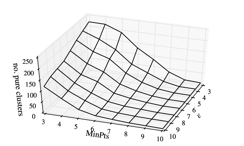
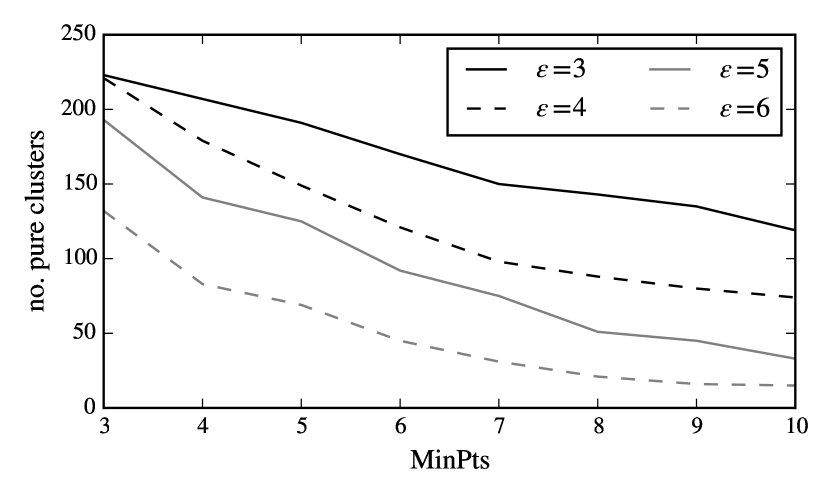
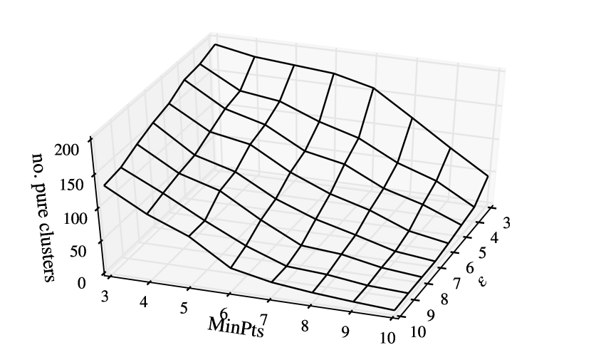
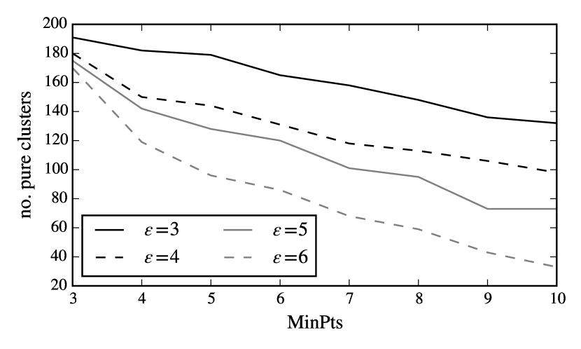
We do not attempt to use hierarchical methods and start with DBSCAN. Previously we have observed that Jaccard is inferior to cosine similarity, and therefore we start directly with cosine.

Like in no-definition case, we calculate the cosine similarity on document vectors where elements are weighed with $(\log\text{TF})\times\text{IDF}$. Using definitions it gives better results, than just identifiers. For example, for ‘‘Linear regression’’ the closest document is ‘‘Linear predictor function’’ with cosine of 0.62, which is the same result, obtained when no definitions are used. However, for ‘‘Singular value decomposition’’ the most similar document is ‘‘Moore–Penrose pseudoinverse’’ with cosine score of 0.386, and this is more meaningful than the most similar document when no definitions are used. As previously, we applied SNN DBSCAN with 10 and 15 nearest neighbors, and the best result was obtained with 10 nearest neighbors, $\varepsilon=3$ and MinPts$=3$ (see fig. 20). It was able to discover 223 namespace-defining clusters, which is slightly better than the best case when no definitions are used.

With MiniBatch $K$-Means applied on the plain untransformed document space we are able to find some interesting clusters, but it general, similarity to the no-definition case, the does not show good results overall. Therefore we apply it to the LSA space reduced by SVD, when identifier-document matrix is reduced to rank $k$. We search for the best combination trying $K=[500;15000]$ and $k\in\{150,250,350\}$. Unlike the case where no definitions are used, the space produced by the soft definition association is affected by $k$ (see fig. 21) and the results produced by $k=350$ are almost always better. The weighing scheme used for this experiment is $(\log\text{TF})\times\text{IDF}$.

Figure 21: Number of discovered pure clusters in $K$-Means and SVD for different number of clusters $K$ and rank $k$.

Figure 22: The effect of rank $k$ used in NMF on $K$-Means.

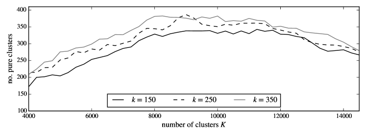
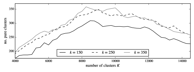
Non-Negative Matrix Factorization gives good results, but does not improve on the best result obtained with SVD (see fig. 22). The largest number of namespace-defining clusters is 370 and it is achieved with $K=10000$ and $k=350$.

Figure 23: The effect of using different weighting systems on $K$-Means with SVD ($k=150$).

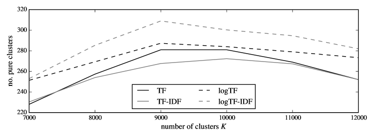
We also experiment with different weighting schemes, and, unlike the no-definition case, it has a significant effect on the results: we can observe that sublinear TF is better that untransformed TF, and $(\log\text{TF})\times\text{IDF}$ achieves the best performance (see fig. 23).

5.2.4 Strong Association

In the case when we use the strong association, the identifier-document matrix has the dimensionality of $37879\times 22512$ identifier-document matrix. It has 499070 entries, so the density of this matrix is just 0.00058.

Like for the soft association case, we choose not to perform usual $K$-Means, and instead proceed directly to MiniBatch $K$-Means on the LSA space reduced with SVD. With rank $k=500$ and number of clusters $K=8250$ is achieves the best result of 340 clusters (see fig. 24), which is slightly worse than in the weak association case. The purity of obtained clustering is 0.5683.

Figure 24: Number of discovered pure clusters in $K$-Means and SVD for different number of clusters $K$ and rank $k$.

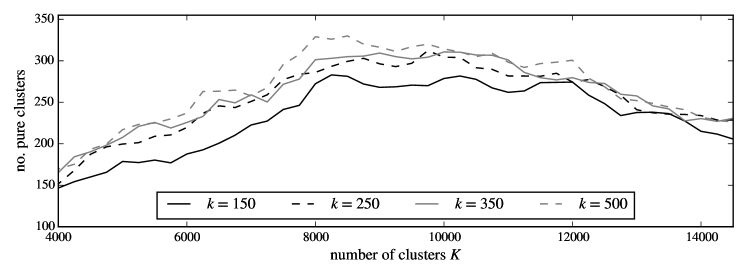
We do not attempt to perform Non-Negative Matrix Factorization as we have previously established that it usually does not give better results while taking significantly longer time.

5.2.5 Russian Wikipedia

Based on the experiments we have performed on the English Wikipedia, we see that the best performance is obtained with weak association by using MiniBatch $K$-Means on LSA space reduced by SVD. We apply the same best performing technique on the Russian Wikipedia.

The identifier-document matrix has the dimensionality of $3948\times 5319$ with 79171 non-zero elements, so the density of this matrix is 0.0038.

Figure 25: Performace of $K$-Means with SVD for Russian Wikipedia.

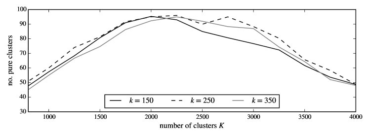
As usually, we applied SVD with different values of rank $k\in\{150,250,350\}$, and, similarity to no-definitions case for the English Wikipedia, we do not observe significant differences across different values of $k$ (see fig. 25). The best achieved result is 105 namespace-defining clusters.

5.3 Result Analysis

5.3.1 English Wikipedia

In the previous chapter we have established that the best way to incorporate definitions into Intensifier Vector Space is by using soft association, and the best clustering performing method is MiniBatch $K$-Means.

Name	Size	Purity
Astronomical catalogues	53	0.9811
Statistics	20	0.8500
Category theory	16	0.8125
Electromagnetism	12	0.8333
Thermodynamics	11	0.8182
Mathematical analysis	11	0.8182
Graph theory	10	0.9000
Graph algorithms	10	0.8000
Fluid dynamics	10	1.0000
Numerical analysis	9	0.8889
Group theory	9	1.0000
Stochastic processes	9	1.0000
Measure theory	8	1.0000

Table 3: Top namespace-defining clusters.

Article	Identifiers
Diagonalizable matrix	$v_{1},\lambda_{1},v_{k},\lambda_{3},\lambda_{2},\lambda_{i},\lambda_{k},\lambda_{j},\lambda_{n},...$
Eigenvalues and eigenvectors	$v_{i},\mu_{A},\lambda_{i},d,\lambda_{n},...$
Principal axis theorem	$v_{1},u_{1},\lambda_{1},\lambda_{2},D,S,u,...$
Eigendecomposition of a matrix	$\lambda,\lambda_{1},\lambda,\lambda_{2},\lambda_{k},R,U,T,...$
Min-max theorem	$\sigma,u_{n},u_{k},u_{i},u_{1},\alpha,\lambda_{1},\lambda,\lambda_{i},...$
Linear independence	$\Lambda,v_{j},u_{2},v_{3},u_{n},\lambda_{1},\lambda_{3},\lambda_{2},...$
Symmetric matrix	$\Lambda,\lambda_{1},\lambda_{2},D,Q,P,\lambda_{i},...$

(a) Wiki Articles in the cluster ‘‘Linear Algebra’’

ID	Definition	Score
$D$	diagonal matrix	0.72
$t$	real argument	0.46
$u$	eigenvalues	0.42
$u_{i}$	eigenvector	0.42
$v_{1}$	eigenvectors	0.73
$\Lambda$	diagonal matrix	0.87
$\lambda$	eigenvalue	0.4
$\lambda_{1}$	eigenvalues	0.95
$\lambda_{2}$	eigenvalues	0.71
$\lambda_{3}$	eigenvalues	0.39
$\lambda_{i}$	eigenvalue	0.98

(b) Definitions in ‘‘Linear Algebra’’

Table 4: A ‘‘Linear Algebra’’ cluster.

$\lambda$
Size	Namespace Name	Definition	Score
3	Algebra	multiplicity	0.43
4	Analysis of variance	marquardt	0.69
3	Applied and interdisciplinary physics	wavelength	0.98
6	Cartographic projections	longitude	1.00
3	Cartography	longitude	1.00
3	Category theory	natural isomorphisms	0.40
4	Condensed matter physics	penetration depth	0.44
5	Continuous distributions	affine parameter	0.46
3	Coordinate systems	longitude	0.88
3	Differential equations	differential operator	0.42
8	Differential geometry	vector fields	0.72
7	Electronic amplifiers	typical value	0.43
3	Electrostatics	unit length	0.43
10	Fluid dynamics	wavelength	1.00
6	Fluid dynamics	free path	0.43
3	Infinity	limit ordinals	0.87
7	Linear algebra	eigenvalue	0.4
5	Linear algebra	matrix	0.41
3	Linear algebra	eigenvalue	0.85
3	Liquids	relaxation time	0.41
3	Materials science	rate	0.44
3	Mathematical analysis	eigenvalue	0.41
3	Mathematical theorems	poisson distribution	0.41
4	Measure theory	lebesgue measure	0.44
3	Measurement	order	0.42
8	Mechanics	previous expression	0.44
4	Mechanics	power series	0.41
3	Metalogic	empty word	0.45
7	Number theory	partition	0.74
4	Number theory	modular lambda function	0.46
3	Operator theory	algebraic multiplicity	0.44
5	Optics	wavelength	0.71
5	Partial differential equations	constants	0.41
4	Physical optics	wavelength	0.95
5	Physics	exciton state	0.88
6	Probability distributions	references	0.42
4	Quantum field theory	coupling constant	0.75
5	Quantum mechanics	wavelength	1.00
5	Quantum mechanics	state	0.87
3	Radioactivity	decay	0.72
4	Representation theory of Lie groups	weight	1.00
3	Riemannian geometry	contravariant vector field	0.45
4	Rubber properties	engineering strain	1.00
3	Statistical data types	regularization parameter	0.45
20	Statistics	words	0.43
3	Statistics	expectation	0.46
3	Stellar astronomy	mean free path	0.43
3	Surface chemistry	ideal gas	0.39
3	Theoretical physics	eigenvalue	0.88
5	Theories of gravitation	dicke	0.44
3	Wave mechanics	wavelength	0.8

Table 5: Some of definitions of ‘‘$\lambda$’’.

The best result is 414 namespace-defining clusters, it is ten times better than the baseline result. The result is achieved by $K$-Means with soft association using parameters $K=9750$ and $k=350$. The purity of this clustering is $0.63$. The largest namespace-defining clusters discovered by this methods are presented in the table 3.

Let us consider a ‘‘Linear Algebra’’ cluster (table 4) with 6 documents and some of extracted definitions in documents of this cluster, and all these articles share identifers $\lambda_{1}$, $m$ and $n$. Let us consider all definitions of identifier ‘‘$\lambda$’’. In total, there are 93 clusters where ‘‘$\lambda$’’ is used (see table 5), and in many cases it is possible to determine that the assignment is correct (e.g. ‘‘eigenvalue’’, ‘‘wavelength’’, ‘‘regularization parameter’’). Some cases are not correct, for example, when we have clusters with the same name where $\lambda$ denotes different things (e.g. in two ‘‘Quantum Mechanics’’ clusters), or in the case of ‘‘Linear Algebra’’ cluster where it denotes a matrix.

Clustering results with sort association are better than results obtained with hard association. One of the reasons for that can the the fact that definitions may act as keywords that describe the document and they are better in describing the semantic content of the document.

Additionally, we see that clustering on the reduced space works better, and in our case the best dimensionality reduction method is SVD.

We also note that we do not discover many namespace-defining clusters. The best result identifiers 414 clusters, while the desired number of clusters $K$ is almost 10 000. It means that information from about 9 000 clusters is discarded: in total there are 22 512 documents, but identifiers from only 1 773 are used, and the rest of the document (about 92%) are not utilized at all.

5.3.2 Russian Wikipedia

For the Russian Wikipedia, the best results is 105 namespace-defining clusters with overall purity of 0.73. It was obtained by $K=3000$ and $k=250$. The largest namespace-defining clusters are shown in table 6. Interestingly, there is a cluster ‘‘Животные’’ (‘‘Animals’’) where mathematical formulae are used to describe ‘‘tooth formula’’. Let us consider a cluster about Linear Algebra (see table 7(a)) and definitions extracted from it (see table 7(a)). Similarity to English Wikipedia, some of the definitions are correct and valid, for example, ‘‘сингулярный число’’ (‘‘singular value’’) for ‘‘$\sigma$’’ or ‘‘ранг’’ (‘‘rank’’) for ‘‘$r$’’, while some are not quite correct, e.g. ‘‘скаляр’’ (‘‘scalar’’) for ‘‘$\lambda$’’. Additionally, some of the non-valid definitions seem to result from misclassifications by the POS-tagger, for example, ‘‘$\Sigma$’’ is defined as ‘‘вдоль’’ (literally ‘‘along’’), which do not make much sense. Furthermore, we can look at all definitions of ‘‘$\lambda$’’ across all discovered namespaces (see table 7(c)). The scores of namespace relations extracted from Russian wikipedia are generally smaller than in English, but it is most likely because there are fewer relations in the Russian dataset.

For the Russian part of Wikipedia, we also utilize just 382 documents, which is only 7%, and the rest of the documents (93%) are filtered out.

Article (Original name)	Article (English)	Size	Purity
Общая алгебра	Algebra	7	0.8571
Диф. геометрия и топология	Differential geometry and topology	7	1.0000
Диф. геометрия и топология	Differential geometry and topology	6	0.8333
Функциональный анализ	Functional analysis	6	0.8333
Животные	Animals	6	0.8333
Картография	Cartography	6	1.0000
Математический анализ	Mathematical analysis	5	1.0000
Математический анализ	Mathematical analysis	5	0.8000
Теория вероятностей	Probability theory	5	1.0000
Механика	Mechanics	5	0.8000
Диф. уравнения в частных производных	Partial differential equations	5	0.8000
Математический анализ	Mathematical analysis	5	0.8000
Релятивистские и гравитационные явления	Relativity and gravitation	5	0.8000
Линейная алгебра	Linear algebra	5	1.0000
Математический анализ	Mathematical analysis	5	1.0000
Физика твёрдого тела	Solid-state physics	5	0.8000

Table 6: Largest namespace-defining clusters extracted from Russian Wikipedia.

Article (Original name)	Article (English)	Identifiers
Линейная алгебра	Linear algebra	$V,v_{n},\alpha,v_{1},v_{2},x,\alpha_{1},\beta,\lambda,f,U,...$
Спектральная теорема	Spectral theorem	$\Lambda,\lambda,H,K,P,U,T,V,X,f,y,x,...$
Сингулярное разложение	Singular value decomposition	$\Sigma,V_{k},\sigma,M,U,T,V,k,r,u,v,...$
Ковариантность и контравариантность	Covariance and contra-variance	$S,V,d,g,f,k,m,f_{i},n,u,v,x,...$
Теорема Куранта – Фишера	Courant–Fischer theorem	$k,V,S,L_{k},...$

(a) A namespace-defining cluster about Linear algebra.

ID	Definition	Definition (English)	Score
$H$	гильбертов	hilbert	0.44
$L$	отображение	transformation	0.95
$L_{k}$	оператор	operator	0.41
$M$	воздействие матрица	matrix	0.71
$T$	линейный отображение	linear transformation	0.43
$U$	унитарный матрица	unitary matrix	0.71
$V$	пространство	space	0.99
$g$	билинейный форма	bilinear form	0.71
$r$	ранг	rank	0.46
$x$	собственный вектор	eigenvector	0.44
$\Lambda$	диагональный матрица	diagonal matrix	0.88
$\Sigma$	вдоль	‘‘along’’	0.44
$\lambda$	скаляр	scalar	0.46
$\sigma$	сингулярный число	singular value	0.45

(b) Definitions in the ‘‘Linear Algebra’’ namespace.

$\lambda$
Size	Original name	English name	Original definition	English definition	Score
3	Алгебра	Algebra	поль	field	0.74
5	Гидродинамика	Fluid dynamics	тепловой движение	thermal motion	0.42
4	Гравитация	Gravitation	коэф. затухание	damping coefficient	0.46
6	Картография	Cartography	долгота	longitude	0.98
5	Линейная алгебра	Linear algebra	скаляр	scalar	0.46
4	Оптика	Optics	длина	length	0.88
3	Оптика	Optics	длина волна	wavelength	0.44
5	Релятивистские и гравитационные явления	Relativity and gravitation	частота	frequency	0.42
3	Статистическая физика	Statistical physics	итоговый выражение	final expression	0.42
3	Теоремы комплексного анализа	Theorems of complex analysis	нуль порядок	‘‘zero order’’	0.45
3	Теория алгоритмов	Algorithms	функция переход	transition function	0.89
5	Физические науки	Physical sciences	длина	length	0.43

(c) Definitions of ‘‘$\lambda$’’ across all namespaces.

Table 7: Namespaces extracted from Russian wikipedia.

5.4 Building Hierarchy

After the namespaces are found, we need to organize them into a hierarchical structure. It is hard to do automatically, and we choose to use existing hierarchies for mathematical knowledge, and then map the found namespaces to these hierarchies.

The first hierarchy that we use is ‘‘Mathematics Subject Classification’’ (MSC) hierarchy [67] by the American Mathematical Society, and it is used for categorizing mathematical articles. In this scheme there are 64 top-level categories such as ‘‘Mathematical logic’’, ‘‘Number theory’’, or ‘‘Fourier analysis’’. It also includes some physics categories such as ‘‘Fluid mechanics’’ or ‘‘Quantum Theory’’. The following top level categories are excluded: ‘‘General’’, ‘‘History and biography’’ and ‘‘Mathematics education’’.

Each top-level category contains second-level categories and third-level categories. In this work we exclude all subcategories those code ends with 99: they are usually ‘‘Miscellaneous topics’’ or ‘‘None of the above, but in this section’’.

Additionally, we excluded the following second level categories because they interfere with PACS, a different hierarchy for Physics:

• Quantum theory $\to$ Axiomatics, foundations, philosophy

• Quantum theory $\to$ Applications to specific physical systems

• Quantum theory $\to$ Groups and algebras in quantum theory

• Partial differential equations $\to$ Equations of mathematical physics and other areas of application

The second hierarchy is ‘‘Physics and Astronomy Classification Scheme’’ (PACS) [68], which is a scheme for categorizing articles about Physics. Like in MSC, we remove the top-level category ‘‘GENERAL’’.

Finally, we also use the ACM Classification Scheme [69] available as a SKOS [70] ontology at their website. The SKOS ontology graph was processed with RDFLib [71]. We use the following top level categories: ‘‘Hardware’’, ‘‘Computer systems organization’’, ‘‘Networks’’, ‘‘Software and its engineering’’, ‘‘Theory of computation’’, ‘‘Information systems’’, ‘‘Security and privacy’’, ‘‘Human-centered computing’’, ‘‘Computing methodologies’’.

After obtaining and processing the data, the three hierarchies are merged into one.

However these categories are only good for English articles and a different hierarchy is needed for Russian. One of such hierarchies is ‘‘Государственный рубрикатор научно-технической информации’’ (ГРНТИ) – ‘‘State categorizator of scientific and technical information’’, which is a state-recommended scheme for categorizing scientific articles published in Russian [72]. The hierarchy is extracted from the official website. It provides a very general categorization and therefore we keep only the following math-related categories: ‘‘Астрономия’’ (‘‘Astronomy’’), ‘‘Биология’’ (‘‘Biology’’), ‘‘Информатика’’ (‘‘Informatics’’), ‘‘Математика’’ (‘‘Mathematics’’), ‘‘Механика’’ (‘‘Mechanics’’), ‘‘Статистика’’ (‘‘Statistics’’), ‘‘Физика’’ (‘‘Physics’’), ‘‘Химия’’ (‘‘Chemistry’’), ‘‘Экономика. Экономические Науки’’ (‘‘Economics’’) and others.

Once the hierarchy is established, each found namespace is mapped to the most suitable second-level category. This is done by keywords matching. First, we extract all key words from the category, which includes top level category name, subcategory name and all third level categories. Then we also extract the category information from the namespace, but we also use the names of the articles that form the namespace. Finally, the keyword matching is done by using the cosine similarity between the cluster and each category. The namespace is assigned to the category with the best (largest) cosine score.

If the cosine score is low (below $0.2$) or there is only one keyword matched, then the cluster is assigned to the ‘‘OTHERS’’ category.

For example, consider a namespace derived from the cluster consisting of ‘‘Tautology (logic)’’, ‘‘List of logic systems’’, ‘‘Regular modal logic’’ ‘‘Combinational logic’’ documents. Among others, these articles belong to categories ‘‘Mathematical logic’’ and ‘‘Logic’’. Then the following is the list of keywords extracted from the cluster: ‘‘tautology’’, ‘‘logic’’, ‘‘list’’, ‘‘systems’’, ‘‘regular’’, ‘‘modal’’, ‘‘combinational’’, ‘‘logical’’, ‘‘expressions’’, ‘‘formal’’, ‘‘propositional’’, ‘‘calculus’’ and so on. Apparently, this namespace is about mathematical logic.

Then consider a list of keywords for ‘‘’General logic’’, a subcategory of ‘‘Mathematical logic and foundations’’ from MSC: ‘‘mathematical’’, ‘‘logic’’, ‘‘foundations’’, ‘‘general’’, ‘‘classical’’, ‘‘propositional’’, ‘‘type’’, ‘‘subsystems’’ and others.

These keywords are represented as vectors in a vector space and the cosine score between these vectors is calculated. For this example, the cosine is approximately 0.75, and this is the largest similarity, and therefore this namespace is mapped to the ‘‘General logic’’ subcategory.

Let us consider the namespaces discovered from the English Wikipedia. The majority of namespaces are mapped correctly. For example:

• ATOMIC AND MOLECULAR PHYSICS

  • Atomic properties and interactions with photons (wiki: Atomic physics; Quantum mechanics; Atomic, molecular, and optical physics)

• Algebraic geometry

  • Computational aspects in algebraic geometry (wiki: Sheaf theory, Theorems in geometry, Theorems in algebraic geometry

  • Computational aspects in algebraic geometry (wiki: Algebraic geometry, Algebraic varieties, Manifolds)

  • Surfaces and higher-dimensional varieties (wiki: Algebraic varieties, Threefolds, Surfaces

• Algebraic topology

  • Fiber spaces and bundles (wiki: Differential geometry, Fiber bundles, Topology)

  • Spectral sequences (wiki: Abstract algebra, Homological algebra, Algebraic topology)

  • Applied homological algebra and category theory (wiki: Continuous mappings, Algebraic topology, Homotopy theory)

• Biology and other natural sciences

  • Mathematical biology in general (wiki: Evidence-based practices, Public health, Epidemiology)

  • Genetics and population dynamics (wiki: Population genetics, Genetics, Subfields and areas of study related to evolutionary biology)

• Computing methodologies

  • Machine learning (wiki: Machine learning, Learning, Artificial intelligence)

  • Machine learning (wiki: Statistical data types, Multivariate statistics, Statistical classification)

• Information systems

  • Data management systems (wiki: Databases, Information technology management, Computer data)

However, some of the mapped namespaces are only partially accurate:

• Computer systems organization

  • Real-time systems (wiki: Computer languages, Type systems, Data types; matched keywords: languages computer systems architecture)

• Fluid mechanics

  • Biological fluid mechanics (wiki: Fluid mechanics, Soft matter, Gases; matched keywords: mechanics fluid)

  • Biological fluid mechanics (wiki: Fluid dynamics, Fluid mechanics, Computational fluid dynamics; matched keywords: mechanics fluid)

• Functional analysis

  • Distributions, generalized functions, distribution spaces (wiki: Probability distributions, Exponential family distributions, Continuous distributions; matched keywords: analytic distribution distributions generalized)

• $K$-theory

  • Whitehead groups and $K_{1}$ (wiki: Group theory, Subgroup properties, Metric geometry; matched keywords: group subgroup)

• Partial differential equations

  • Close-to-elliptic equations (wiki: Differential equations, Numerical analysis, Numerical differential equations; matched keywords: partial differential equations)

Finally, namespaces marked as ‘‘OTHER’’ are usually matched incorrectly:

• OTHER

  • Randomness, geometry and discrete structures (wiki: Coordinate systems, Cartography, Cartographic projections; matched keywords: projections)

  • Other generalizations (wiki: Electrostatics, Concepts in physics, Electromagnetism; matched keywords: potential)

  • Computational methods (wiki: General relativity, Exact solutions in general relativity, Equations; matched keywords: relativity)

  • Other classes of algebras (wiki: International sailing classes, Keelboats, Olympic sailboat classes; matched keywords: classes)

For the Russian version of Wikipedia, the majority of namespaces are also mapped correctly. For example:

• АСТРОНОМИЯ (ASTRONOMY)

  • Звезды (Stars) (wiki: Физические науки (Physical sciences), Астрофизика (Astrophysics), Астрономия (Astronomy))

• ГЕОФИЗИКА (GEOPHYSICS)

  • Океанология (Oceanology) (wiki: Океанология (Oceanology), Физическая география (Physical geography), Гидрология (Hydrology))

• КИБЕРНЕТИКА (CYBERNETICS)

  • Теория информации (Information theory) (wiki: Цифровые системы (Digital systems), Теория информации (Information theory), Теория кодирования (Coding theory))

  • Теория конечных автоматов и формальных языков (Finite state automata and formal languages) (wiki: Теория алгоритмов (Algorithmic theory), Теория автоматов (Automata theory), Визуализация данных (Data visualization))

• МАТЕМАТИКА (MATHEMATICS)

  • Математический анализ (Mathematical analysis) (wiki: Математический анализ (Mathematical analysis), Разделы математики (Parts of mathematics), Функциональный анализ (Functional analysis))

  • Теория вероятностей и математическая статистика (Probability and statistics) (wiki: Теория вероятностей (Probability), Теория вероятностей и математическая статистика (Probability and statistics), Теория меры (Measure theory))

  • Основания математики и математическая логика (Foundation of mathematics and mathematica logics) (wiki: Логика (Logic), Разделы математики (Parts of mathematics), Математика (Mathematics))

  • Алгебра (Algebra) (wiki: Теория колец (Rings Theory), Теория полей (Fields Theory), Теория групп (Groups Theory))

• МЕТРОЛОГИЯ (METROLOGY)

  • Измерения отдельных величин и характеристик (Measurements of individual values and characteristics) (wiki: Единицы измерения (Units of measure), Системы мер (Measure systems), Макс Планк (Max Plank))

• ФИЗИКА (PHYSICS)

  • Физика элементарных частиц. Теория полей. Физика высоких энергий (Particle physics. Field theory. High-energy physics) (wiki: Гравитация (Gravity), Классическая механика (Classical mechanics), Классическая физика (Classical physics))

  • Физика твердых тел (Physics of solids) (wiki: Физика конденсированного состояния (Condensed matter physics), Кристаллография (Crystallography), Физика твёрдого тела (Physics of solids))

  • Оптика (Optics) (wiki: Оптика (Optics), Физические науки (Physical sciences), Методы экспериментальной физики (Methods of experimental physics))

5.5 Evaluation Summary

The best definition embedding technique is soft association. The best clustering algorithm is $K$-Means with $K=9500$ on the semantic space produced by rank-reduced SVD with $k=250$ with TF-IDF weight where TF is sublinear.

We used ‘‘$E=mc^{2}$’’ as a motivating example for namespace discovery. When namespaces are discovered, we can look at how the identifiers ‘‘$E$’’, ‘‘$m$’’, ‘‘$c$’’ are used in different namespaces. Additionally, we can look at other common identifiers such as ‘‘$\lambda$’’, ‘‘$\sigma$’’ and ‘‘$\mu$’’ (see table 8). We see that definitions of ‘‘$E$’’, ‘‘$m$’’, ‘‘$c$’’ are correct for the ‘‘General relativity’’ namespace, and ‘‘$E$’’ is ‘‘expectation’’ for the ‘‘Probability’’ namespace, however we have not observed that ‘‘$E$’’ is ‘‘Elimination matrix’’ for the ‘‘Linear algebra’’ namespaces, but it is just ‘‘matrix’’.

We also repeat this experiment for the Russian Wikipedia (table 9), but chose slightly different namespaces. Similarly to English Wikipedia, ‘‘$E$’’, ‘‘$m$’’, ‘‘$c$’’ are discover correctly, but nothing is discovered for ‘‘$E$’’ in namespaces about probability and linear algebra.

$E$ $m$ $c$ $\lambda$ $\sigma$ $\mu$ Linear algebra matrix matrix scalar eigenvalue related permutation algebraic multiplicity General relativity energy mass speed of light length shear reduced mass Coding theory encoding function message transmitted codeword natural isomorphisms Optics order fringe speed of light in vacuum wavelength conductivity permeability Probability expectation sample size affine parameter variance mean vector

Table 8: Definitions for selected identifiers and namespaces extracted from the English Wikipedia.

$E$ $m$ $c$ $\lambda$ $\sigma$ $\mu$ Линейная алгебра (Linear algebra) смена базис (change of basis) скаляр (scalar) сингулярный число (singular value) Физические науки (Physical sciences) энергия (energy) масса частицы (mass of particle) скорость свет (speed of light) длина (length) привести масса (reduced mass) Вероятность (Probability) дисперсия (variance) среднее (mean)

Table 9: Definitions for selected identifiers and namespaces extracted from the Russian Wikipedia.

To visualize the discovered namespaces, we first map them to a hierarchy as previously described in section 5.4, and then find the most frequent categories according to this hierarchy. Then, for each category, we rank all discovered identifier-definitions pairs, and show only the most highly ranked ones (see table 10). Additionally, we show the most frequent Wikipedia categories that the documents inside the namespaces have, and also the most influential documents: the ones that contain more identifiers than others. We also repeat the same for Russian Wikipedia (see table 11).

We can note that the top discovered namespaces are quite different across the two datasets, and there is no single namespace among the top namespaces that both datasets share. However, ‘‘Group theory and generalizations’’ and ‘‘Алгебра’’ (‘‘Algebra’’) look a little similar and share a few identifiers. It is probably due to the fact that the datasets may be different in the content and have different distribution of categories. Also, the hierarchies matter as well: in case of Russian, the hierarchy is more general, and therefore the matched categories tend to be more general as well.

Freq. Namespaces Definitions Categories Top Articles 10 Physics: Fluid mechanics $\rho$: density, $p$: pressure, $g$: acceleration, $k$: wavenumber, $u$: velocity, $v$: velocity, $\eta$: free surface, $\omega$: angular frequency, $z$: free surface, $\nu$: kinematic viscosity Fluid dynamics; Fluid mechanics; Dynamics; Aerodynamics; Partial differential equations Navier–Stokes equations; Stokes wave; Airy wave theory; Mild-slope equation; Classic energy problem in open-channel flow 9 Algebra: Differential and difference algebra $R$: ring, $k$: field, $D$: city, $K$: field, $x$: polynomials, $\Gamma$: value group, $M$: submodule, $n$: matrix, $S$: ring, $v$: valuation Abstract algebra; Algebra; Functions and mappings; Polynomials; Analytic functions Recurrence relation; Spectral radius; Levi-Civita symbol; Perron–Frobenius theorem; Leibniz formula for determinants 9 Mathematical analysis: Partial differential equations $\Omega$: domain, $t$: time, $L$: space, $p$: space, $\omega$: angular frequency, $V$: hilbert space, $D$: domain, $u$: horizontal velocity, $x$: time, $U$: velocity profiles Partial differential equations; Differential equations; Multivariable calculus; Mathematical analysis; Fluid dynamics Orr–Sommerfeld equation; Helmholtz equation; Fictitious domain method; Green’s function for the three-variable Laplace equation; Eikonal equation 8 Economics: Mathematical economics $K$: strike, $P$: price level, $p$: probability, $u$: utility, $V$: money, $M$: money, $\alpha$: confidence level, $g$: distortion function, $\sigma$: volatility, $R_{f}$: return Economics; Financial economics; Microeconomics; Mathematical finance; Economic theories Modern portfolio theory; Lookback option; Binary option; Equation of exchange; Slutsky equation 8 Probability theory $X$: process, $t$: time, $X_{t}$: process, $P$: probability measure, $S$: state space, $s$: stochastic processe, $f$: measurable function, $M$: local martingale, $M_{t}$: local martingale, $W_{t}$: process Stochastic processes; Probability theory; Statistics; Statistical data types; Measure theory Wiener process; Itō calculus; Local martingale; Stratonovich integral; Glivenko–Cantelli theorem 7 Algebra: Group theory and generalizations $G$: group, $H$: subgroup, $Z$: group, $K$: subgroup, $N$: group, $p$: power, $n$: root, $F$: free group, $Q$: extension, $T$: homomorphism Group theory; Abstract algebra; Metric geometry; Algebraic structures; Theorems in group theory Free abelian group; Center (group theory); Holomorph (mathematics); $P$-group; Powerful $p$-group 7 Mathematical logic: General logic $w$: world, $R$: binary relation, $P$: predicate, $Q$: statement, $W$: nodes, $\phi$: modal formula, $n$: natural number, $v$: world, $T$: relation, $k$: degree Mathematical logic; Logic; Proof theory; Syntax (logic); Formal systems Sequent calculus; First-order logic; Original proof of Gödel’s completeness theorem; Kripke semantics; Szpilrajn extension theorem

Table 10: Most frequent definitions in most frequent namespaces extracted from the English Wikipedia.

Freq. Namespaces Definitions Categories Top Articles 10 Алгебра (Algebra) $G$: группа (group), $V$: пространство (space), $p$: простой число (prime number), $K$: подпространство (subspace), $R$: кольцо (ring), $C$: категория (category), $n$: ‘‘o ( n )’’, $F$: поль (field), $L$: линейный пространство (linear space), $D$: категория (category) Действие группы (Group action), Линейная алгебра (Linear algebra), Векторное пространство (Vector space), Алгебра (Algebra), Нормированное пространств (Normed vector space) Общая алгебра (General algebra), Алгебра (algebra), Теория групп (Group theory), Линейная алгебра (Linear algebra), Теория колец (Ring theory) 7 Топология (Topology) $M$: многообразие (manifold), $X$: топологический пространство (topologic space), $n$: многообразие (manifold), $U$: окрестность (neighborhood), $C$: класс (class), $S$: пучок (sheaf), $x$: пространство (space), $k$: ранг (rank), $V$: слой (layer), $f$: степень отображение (degree of mapping) Топология (Topology); Дифференциальная геометрия и топология (Differential geometry and topology); Геометрия (Geometry); Общая топология (General topology); Общая алгебра (General algebra) Параллельное поле (Parallel field); Алгебраическая топология (Algebraic topology); Векторное расслоение (Vector bundle); Когомологии де Рама (De Rham cohomologies); Структура (дифференциальная геометрия) (Structure – differential geometry) 6 Теория вероятностей и математическая статистика (Probability and statistics) $\Omega$: элементарный событие (event), $P$: вероятность (probability), $F$: алгебра событие (event algebra), $X$: случайный величина (random variable), $\omega$: множество элемент (element of set), $g$: интегрировать функция (integrable function), $n$: стремление (convergence), $N$: счётный мера (countable measure), $\sigma$: событие (event), $p$: момент (moment) Теория вероятностей (Probability); Теория вероятностей и математическая статистика (Probability and statistics); Теория меры (Measure theory); Математические теоремы (Mathematical theorems); Теоремы теории вероятностей и математической статистики (Theorems of probability and statistics) Случайная величина (Random variable); Аксиоматика Колмогорова (Kolmogorov axioms); Пространство элементарных событий (Sample space); Теорема Лебега о мажорируемой сходимости (Lebesgue’s dominated convergence theorem); $t$-Критерий Стьюдента (Student’s $t$-test) 5 Физика элементарных частиц. Теория полей. Физика высоких энергий (Particle physics. Field theory. High energy physics) $G$: гравитационный постоянный (gravitation constant), $M$: масса (mass), $c$: скорость свет (speed of light), $m_{2}$: масса (mass), $m$: масса (mass), $\Psi$: волновой функция (wave function), $m_{1}$: материальный точка масса (mass of material point), $t$: время (time), $r$: расстояние (distance), $R$: масса (mass) Гравитация (Gravitation); Астрономия (Astronomy); Общая теория относительности (General relativity); Теория относительности (Relativity theory); Физическая космология (Physical cosmology) Чёрная дыра (Black hole); Гравитационное красное смещение (Gravitational redshift); Квантовый компьютер (Quantum computer); Метрика Шварцшильда (Schwarzschild metric); Гравитация (Gravitation) 5 Оптика (Optics) $\Phi_{0}$: поток излучение (Radiant flux), $\lambda$: длина (length), $\Phi$: поток излучение (Radiant flux), $l$: расстояние (distance), $\varepsilon$: приёмник (‘‘receiver’’), $n_{1}$: показатель преломление (refractive index), $K_{m}$: световой эффективность излучение (luminous efficacy), $n$: показатель преломление (refractive index), $n_{2}$: преломление среда (‘‘refractive environment’’), $r$: рассеяние (dispersion) Оптика (Optics); Физические науки (Physical sciences); Волновая физика (Wave mechanics); Фотометрия (Photometry); Методы экспериментальной физики (Methods of experimental physics) Энергия излучения (оптика) (Radiant energy); Облучённость (фотометрия) (Irradiance); Фотонный кристалл (Photonic crystal); Свет (Light); Сила излучения (фотометрия) (Radiant intensity)

Table 11: Most frequent definitions in most frequent namespaces extracted from the Russian Wikipedia.

6 Conclusions

The goal of this work was to discover namespaces in mathematical notation given a collection of documents with mathematical formulae. This problem could not be performed manually: this task it too time consuming and requires a lot of effort.

To achieve the goal we proposed an automatic method based on cluster analysis. We noted that document representation in terms of identifiers is similar to the classic Vector Space Model. This allowed us to apply traditional document clustering techniques to the namespace discovery problem.

We expected to discover namespaces, that are homogenies and corresponded to the same area of knowledge. The clusters that we discovered are homogenous, but not all corresponded to the same category. This is why we additionally used the category information to recognize the namespaces-defining clusters amount all clusters, and then we built namespaces from them.

We also initially expected that there would be more namespace-defining clusters, but in our results the majority of clusters are not ‘‘pure’’: documents inside these clusters do not belong to the same category. These clusters are only homogenous in the cluster analysis sense: the within-cluster distances is minimal.

To prove that namespace discovery is possible in principle, we first applied the proposed method to a dataset where the ‘‘gold standard’’ is known: to Java source code, and we were able to partially recover the namespaces using only the information about identifiers.

Then we used the method to extract namespaces from the English Wikipedia, and we were able to discover 414 namepaces from this dataset. This result is better than random guessing by the factor of ten. We observed that dimensionality reduction techniques are very helpful, and clustering algorithms work better on the reduce space. MiniBatch $K$-Means algorithms shows the best results for discovering namespace-defining clusters.

Additionally, we applied the same method to the Russian version of Wikipedia, and, although the distribution of most frequent namespaces are different in these two datasets, the overall results are consistent.

The problem of namespace discovery has not been studied before, and there was no dataset where identifiers were assigned to namespaces. In this work we showed that the automatic namespace discovery is possible, and it is a good start.

However, there are many ways in which the present approach can be improved further. In the next section we discuss possible directions.

7 Outlook and Future Work

7.1 Implementation and Other Algorithms

We use the Probabilistic approach to extracting definitions for identifiers, and it is good because it requires almost no parameter tuning. While this approach works well most of the time, sometimes we observe some false positives, most likely due to the fact that the dataset is quite noisy. It potentially can be improved by using some Machine Learning method, which, however, may require creating a hand-labeled dataset with identifier-definition relations. To facilitate the creation of such a dataset it is possible to pre-generate some data using using the current approach for further labeling.

In the experiments section we have observed that cluster algorithms that produce many clusters tend to have good performance. However, they also tend to create related clusters from the same category and with same or similar identifiers and definitions. Therefore such results can be refined further and merged. This can be done, for example, by using the join operation from the Scatter/Gather algorithm [28], which finds the most similar clusters and merges them.

We were not able to apply hierarchical agglomerative clustering algorithms because their time complexity is prohibitive, but they may produce good clusters. For these algorithms we are usually interested in the nearest neighbors of a given data point, and therefore we can use approximation algorithms for computing nearest neighbors such as Locality-Sensitive Hashing (LSH) [73]. The LSH algorithms can be used for text clustering [74], and therefore they should work well for identifiers. Additionally, LSH is also a dimensionality reduction technique, and we have observed that generally reducing dimensionality helps to obtain better clusters.

In this work we use hard assignment clustering algorithms, which means, that a document can import only from one namespace. This assumption does not necessarily always hold true and we may model the fact that documents may import from several namespaces by using Fuzzy Clustering (or Soft Clustering) algorithms [75].

In Latent Semantic Analysis other dimensionality reduction techniques can be used, for example, Local Non-Negative Matrix Factorization [76]. There is also a randomized Non-Negative Matrix Factorization algorithm that uses random projections [77] [78], which potentially can give a speed up while not significantly losing in performance. Another dimensionality reduction technique useful for discovering semantics is Dynamic Auto-Encoders [79].

Additionally, we can try different approaches to clustering such as Spectral Clustering [80] or Micro-Clustering [81].

Finally, topic modeling techniques such as Latent Dirichlet Allocation [82] can be quite useful for modeling namespaces. It can be seen as a ‘‘soft clustering’’ technique and it can naturally model the fact that a document may import from several namespaces.

7.2 Other Concepts

In this work we assume that document can import only from one namespace, but in reality is should be able to import from several namespaces. As discussed, it can be modeled by Fuzzy Clustering. But it also can be achieved by dividing the document in parts (for example, by paragraphs) and then treating each part as an independent document.

For document clustering we only use identifiers, extracted definitions and categories. It is possible to take advantage of additional information from Wikipedia articles. For example, extract some keywords from the articles and use them to get a better cluster assignment.

The Wikipedia data set can be seen as a graph, where two articles have an edge if there is an interwiki link between them. Pages that describe certain namespaces may be quite interconnected, and using this idea it is possible to apply link-based clustering methods (such as ones described in [83] and [84]) to find namespace candidates. There are also hybrid approaches that can use both textual representation and links [21].

Vector Space Model is not the only possible model to represent textual information as vectors. There are other ways to embed textual information into vector spaces like word2vec [85] or GloVe [86], and these methods may be useful for representing identifers and definitions as well.

Tensors may be a better way of representing identifier-definition pairs. For example, we can represent the data set as a 3-dimensional tensor indexed by documents, identifiers and definition. Tensor Factorization methods for revealing semantic information are an active area of research in NLP and linguistics [87], so it is also possible to apply these methods to the namespace discovery problem.

Finally, while running experiments, we observed that sometimes results of clustering algorithms with the same parameters produce quite different results, or some algorithms produce a small amount of good quality namespaces, while others produce many namespaces which may be less coherent. Therefore it can be interesting to investigate how to combine the results of different cluster assignments such that the combined result is better in terms of the number of namespace-defining clusters. One way of achieving this can be building ensembles of clustering algorithms [88]. Alternatively, a special approach for optimizing for the number of pure clusters can be proposed, for example, partially based on the ideas from Boosting [89]: apply a clustering algorithm, remove the discovered pure clusters, and run the algorithm again on the remaining documents until no new clusters are discovered.

7.3 Other Datasets

In this work we use Wikipedia as the data source and extract namespaces from the English part of Wikipedia. Additionally, we also apply the methods to the Russian part, and therefore it shows that it is possible to extract namespaces from Wikipedia in any other available language.

But we can also apply to some other larger dataset, such as arXiv, a repository of over one million of scientific papers in many different areas. The source code of these articles are available in LaTeX, and it can be processed automatically.

There are many scientific Q&A websites on the Internet. The stack exchange is one of the largest Q&A networks, and there are many sites on this network that contain mathematical formulae, such as ‘‘mathematics’’, ‘‘mathoverflow’’, ‘‘cross validated’’, ‘‘data science’’, ‘‘theoretical computer science’’, ‘‘physics’’, ‘‘astronomy’’, ‘‘economics’’ and many others. This network makes their data available for download and it also can be a good data source for namespace discovery. In addition to content, the questions contain a lot of potentially useful metadata such as related questions and tags.

7.4 Unsolved Questions

The most important question is how to extend this method to situations when no additional information about document category is known. To solve it, we need to replace the notion of purity with some other objective for discovering namespace-defining clusters.

Also, a metric for evaluating the quality of a namespace is needed. Now we assume that pure clusters are namespace-defining clusters. But the namespace candidates should adhere to the namespace definition as much as possible, and therefore a good criteria is needed to quantify to what extent the definition is satisfied. This will help to define whether a cluster defines a good namespace or not.

After namespaces are discovered we organize them into hierarchies. To do that we use existing hierarchies, but they are not always complete and there are mismatches. What is more, when this technique is applied to some other language, a different hierarchy is needed for this language, and we experienced it when processing the Russian part of Wikipedia: for that we needed to obtain a special hierarchy. There should be a way of building these hierarchies automatically, without the need of external dataset. Potentially it should be possible to use hierarchical clustering algorithms, but it may result in very deep and unnatural hierarchies, and therefore some additional investigation in this direction may be needed.

8 Bibliography

References

- [1] Erik Duval, Wayne Hodgins, Stuart Sutton, and Stuart L Weibel. Metadata principles and practicalities. D-lib Magazine, 8(4):16, 2002.
- [2] Henry Thompson, Tim Bray, Dave Hollander, Andrew Layman, and Richard Tobin. Namespaces in XML 1.0 (third edition). W3C recommendation, W3C, December 2009. http://www.w3.org/TR/2009/REC-xml-names-20091208/.
- [3] James Gosling, Bill Joy, Guy Steele, Gilad Bracha, and Alex Buckley. The Java 8® Language Specification, Java SE 8 Edition. Addison-Wesley Professional, 2014.
- [4] Wikipedia. Mathematical notation — Wikipedia, the free encyclopedia, 2015. https://en.wikipedia.org/w/index.php?title=Mathematical_notation&oldid=646730035, accessed: 2015-07-01.
- [5] Robert Pagel and Moritz Schubotz. Mathematical language processing project. arXiv preprint arXiv:1407.0167, 2014.
- [6] Anders Møller and Michael I Schwartzbach. An introduction to XML and Web Technologies. Pearson Education, 2006.
- [7] Kevin McArthur. What’s new in PHP 6. Pro PHP: Patterns, Frameworks, Testing and More, pages 41–52, 2008.
- [8] Craig Larman. Applying UML and patterns: an introduction to object-oriented analysis and design and iterative development. Pearson Education India, 2005.
- [9] Dan Jurafsky and James H Martin. Speech & language processing. Pearson Education India, 2000.
- [10] Ulf Schöneberg and Wolfram Sperber. POS tagging and its applications for mathematics. In Intelligent Computer Mathematics, pages 213–223. Springer, 2014.
- [11] Beatrice Santorini. Part-of-speech tagging guidelines for the penn treebank project (3rd revision). 1990.
- [12] Christopher D Manning, Mihai Surdeanu, John Bauer, Jenny Finkel, Steven J Bethard, and David McClosky. The stanford CoreNLP natural language processing toolkit. In Proceedings of 52nd Annual Meeting of the Association for Computational Linguistics: System Demonstrations, pages 55–60, 2014.
- [13] Giovanni Yoko Kristianto, MQ Ngiem, Yuichiroh Matsubayashi, and Akiko Aizawa. Extracting definitions of mathematical expressions in scientific papers. In Proc. of the 26th Annual Conference of JSAI, 2012.
- [14] Mihai Grigore, Magdalena Wolska, and Michael Kohlhase. Towards context-based disambiguation of mathematical expressions. In The Joint Conference of ASCM, pages 262–271, 2009.
- [15] Keisuke Yokoi, Minh-Quoc Nghiem, Yuichiroh Matsubayashi, and Akiko Aizawa. Contextual analysis of mathematical expressions for advanced mathematical search. In Prof. of 12th International Conference on Intelligent Text Processing and Comptational Linguistics (CICLing 2011), Tokyo, Japan, February, pages 20–26, 2011.
- [16] Minh Nghiem Quoc, Keisuke Yokoi, Yuichiroh Matsubayashi, and Akiko Aizawa. Mining coreference relations between formulas and text using Wikipedia. In 23rd International Conference on Computational Linguistics, page 69, 2010.
- [17] Jerzy Trzeciak. Writing mathematical papers in English: a practical guide. European Mathematical Society, 1995.
- [18] Giovanni Yoko Kristianto, Akiko Aizawa, et al. Extracting textual descriptions of mathematical expressions in scientific papers. D-Lib Magazine, 20(11):9, 2014.
- [19] Christopher D Manning, Prabhakar Raghavan, Hinrich Schütze, et al. Introduction to information retrieval, volume 1. Cambridge university press Cambridge, 2008.
- [20] Fabrizio Sebastiani. Machine learning in automated text categorization. ACM computing surveys (CSUR), 34(1):1–47, 2002.
- [21] Nora Oikonomakou and Michalis Vazirgiannis. A review of web document clustering approaches. In Data mining and knowledge discovery handbook, pages 921–943. Springer, 2005.
- [22] Charu C Aggarwal and ChengXiang Zhai. A survey of text clustering algorithms. In Mining Text Data, pages 77–128. Springer, 2012.
- [23] Gerard Salton and Christopher Buckley. Term-weighting approaches in automatic text retrieval. Information processing & management, 24(5):513–523, 1988.
- [24] Levent Ertöz, Michael Steinbach, and Vipin Kumar. Finding clusters of different sizes, shapes, and densities in noisy, high dimensional data. In SDM, pages 47–58. SIAM, 2003.
- [25] Kevin Beyer, Jonathan Goldstein, Raghu Ramakrishnan, and Uri Shaft. When is ‘‘nearest neighbor’’ meaningful? In Database Theory – ICDT’ 99, pages 217–235. Springer, 1999.
- [26] Deborah Hughes-Hallett, William G. McCallum, Andrew M. Gleason, et al. Calculus: Single and Multivariable, 6th Edition. Wiley, 2013.
- [27] Tuomo Korenius, Jorma Laurikkala, and Martti Juhola. On principal component analysis, cosine and euclidean measures in information retrieval. Information Sciences, 177(22):4893–4905, 2007.
- [28] Douglass R Cutting, David R Karger, Jan O Pedersen, and John W Tukey. Scatter/Gather: A cluster-based approach to browsing large document collections. In Proceedings of the 15th annual international ACM SIGIR conference on Research and development in information retrieval, pages 318–329. ACM, 1992.
- [29] Michael Steinbach, George Karypis, Vipin Kumar, et al. A comparison of document clustering techniques. In KDD workshop on text mining, volume 400, pages 525–526. Boston, 2000.
- [30] Rui Xu, Donald Wunsch, et al. Survey of clustering algorithms. Neural Networks, IEEE Transactions on, 16(3):645–678, 2005.
- [31] Mark Hall, Paul Clough, and Mark Stevenson. Evaluating the use of clustering for automatically organising digital library collections. In Theory and Practice of Digital Libraries, pages 323–334. Springer, 2012.
- [32] David Sculley. Web-scale k-means clustering. In Proceedings of the 19th international conference on World wide web, pages 1177–1178. ACM, 2010.
- [33] Hinrich Schütze and Craig Silverstein. Projections for efficient document clustering. In ACM SIGIR Forum, volume 31, pages 74–81. ACM, 1997.
- [34] Martin Ester, Hans-Peter Kriegel, Jörg Sander, and Xiaowei Xu. A density-based algorithm for discovering clusters in large spatial databases with noise. In KDD, volume 96, pages 226–231, 1996.
- [35] Levent Ertöz, Michael Steinbach, and Vipin Kumar. Finding topics in collections of documents: A shared nearest neighbor approach. pages 83–103, 2004.
- [36] Thomas K Landauer, Peter W Foltz, and Darrell Laham. An introduction to latent semantic analysis. Discourse processes, 25(2-3):259–284, 1998.
- [37] Scott C. Deerwester, Susan T Dumais, Thomas K. Landauer, George W. Furnas, and Richard A. Harshman. Indexing by latent semantic analysis. JAsIs, 41(6):391–407, 1990.
- [38] Stanisław Osiński, Jerzy Stefanowski, and Dawid Weiss. Lingo: Search results clustering algorithm based on singular value decomposition. In Intelligent information processing and web mining, pages 359–368. Springer, 2004.
- [39] Nicholas Evangelopoulos, Xiaoni Zhang, and Victor R Prybutok. Latent semantic analysis: five methodological recommendations. European Journal of Information Systems, 21(1):70–86, 2012.
- [40] Stanisław Osiński. Improving quality of search results clustering with approximate matrix factorisations. In Advances in Information Retrieval, pages 167–178. Springer, 2006.
- [41] Daniel D Lee and H Sebastian Seung. Learning the parts of objects by non-negative matrix factorization. Nature, 401(6755):788–791, 1999.
- [42] Wei Xu, Xin Liu, and Yihong Gong. Document clustering based on non-negative matrix factorization. In Proceedings of the 26th annual international ACM SIGIR conference on Research and development in informaion retrieval, pages 267–273. ACM, 2003.
- [43] Eric Evans. Domain-driven design: tackling complexity in the heart of software. Addison-Wesley Professional, 2004.
- [44] Alfio Gliozzo and Carlo Strapparava. Semantic domains in computational linguistics. Springer Science & Business Media, 2009.
- [45] Christopher Stokoe, Michael P Oakes, and John Tait. Word sense disambiguation in information retrieval revisited. In Proceedings of the 26th annual international ACM SIGIR conference on Research and development in informaion retrieval, pages 159–166. ACM, 2003.
- [46] Wikimedia Foundation. Russian wikipedia XML data dump, 2015. http://dumps.wikimedia.org/ruwiki/latest/, downloaded from http://math-ru.wmflabs.org/wiki/, accessed: 2015-07-12.
- [47] Apache Software Foundation. Apache Flink 0.8.1. http://flink.apache.org/, accessed: 2015-01-01.
- [48] David Carlisle, Robert R Miner, and Patrick D F Ion. Mathematical markup language (MathML) version 3.0 2nd edition. W3C recommendation, W3C, April 2014. http://www.w3.org/TR/2014/REC-MathML3-20140410/.
- [49] Ronald Rivest. The MD5 message-digest algorithm. 1992.
- [50] Eclipse Foundation. Mylyn WikiText 1.3.0, 2015. http://projects.eclipse.org/projects/mylyn.docs, accessed: 2015-01-01.
- [51] Kristina Toutanova, Dan Klein, Christopher D Manning, and Yoram Singer. Feature-rich part-of-speech tagging with a cyclic dependency network. In Proceedings of the 2003 Conference of the North American Chapter of the Association for Computational Linguistics on Human Language Technology-Volume 1, pages 173–180. Association for Computational Linguistics, 2003.
- [52] Определение части речи слова на PHP одной функцией (part of speech tagging in PHP in one function), 2012. http://habrahabr.ru/post/152389/, accessed: 2015-07-13.
- [53] Daniel Sonntag. Assessing the quality of natural language text data. In GI Jahrestagung (1), pages 259–263, 2004.
- [54] Julie D Allen et al. The Unicode Standard. Addison-Wesley, 2007.
- [55] Mikhail Korobov. Morphological analyzer and generator for russian and ukrainian languages. arXiv preprint arXiv:1503.07283, 2015.
- [56] Martin F Porter. Snowball: A language for stemming algorithms, 2001.
- [57] Steven Bird. NLTK: the natural language toolkit. In Proceedings of the COLING/ACL on Interactive presentation sessions, pages 69–72. Association for Computational Linguistics, 2006.
- [58] F. Pedregosa, G. Varoquaux, A. Gramfort, V. Michel, B. Thirion, O. Grisel, et al. Scikit-learn: Machine learning in Python. Journal of Machine Learning Research, 12:2825–2830, 2011.
- [59] A Tropp, N Halko, and PG Martinsson. Finding structure with randomness: Stochastic algorithms for constructing approximate matrix decompositions. Technical report, 2009.
- [60] Christian Bizer, Jens Lehmann, Georgi Kobilarov, Sören Auer, and et al. DBpedia – a crystallization point for the web of data. Web Semant., 7(3):154–165, September 2009.
- [61] Gonzalo Navarro. A guided tour to approximate string matching. ACM computing surveys (CSUR), 33(1):31–88, 2001.
- [62] SeatGeek. FuzzyWuzzy 0.6.0. https://pypi.python.org/pypi/fuzzywuzzy/0.6.0, accessed: 2015-07-01.
- [63] S. van der Walt, S.C. Colbert, and G. Varoquaux. The numpy array: A structure for efficient numerical computation. Computing in Science Engineering, 13(2):22–30, March 2011.
- [64] Eric Jones, Travis Oliphant, Pearu Peterson, et al. SciPy: Open source scientific tools for Python, 2001–. http://www.scipy.org/, accessed: 2015-02-01.
- [65] Sreenivasa Viswanadha, Danny van Bruggen, and Nicholas Smith. JavaParser 2.1.0, 2015. http://javaparser.github.io/javaparser/, accessed: 2015-06-15.
- [66] Apache Software Foundation. Apache Mahout 0.10.1. http://mahout.apache.org/, accessed: 2015-06-15.
- [67] American Mathematical Society. AMS mathematics subject classification 2010, 2009. http://msc2010.org/, accessed: 2015-06-01.
- [68] American Physical Society. PACS 2010 regular edition, 2009. http://www.aip.org/publishing/pacs/pacs-2010-regular-edition/, accessed: 2015-06-01.
- [69] Bernard Rous. Major update to ACM’s computing classification system. Commun. ACM, 55(11):12–12, November 2012.
- [70] Alistair Miles, Brian Matthews, Michael Wilson, and Dan Brickley. SKOS Core: Simple knowledge organisation for the web. In Proceedings of the 2005 International Conference on Dublin Core and Metadata Applications: Vocabularies in Practice, DCMI ’05, pages 1:1–1:9. Dublin Core Metadata Initiative, 2005.
- [71] Daniel Krech. RDFLib 4.2.0. https://rdflib.readthedocs.org/en/latest/, accessed: 2015-06-01.
- [72] V. I. Feodosimov. Государственный рубрикатор научно-технической информации (state categorizator of scientific and technical information). 2000.
- [73] Jure Leskovec, Anand Rajaraman, and Jeffrey Ullman. Mining of massive datasets, 2nd edition. Cambridge University Press Cambridge, 2014.
- [74] Deepak Ravichandran, Patrick Pantel, and Eduard Hovy. Randomized algorithms and nlp: using locality sensitive hash function for high speed noun clustering. In Proceedings of the 43rd Annual Meeting on Association for Computational Linguistics, pages 622–629. Association for Computational Linguistics, 2005.
- [75] Andrea Baraldi and Palma Blonda. A survey of fuzzy clustering algorithms for pattern recognition. i. Systems, Man, and Cybernetics, Part B: Cybernetics, IEEE Transactions on, 29(6):778–785, 1999.
- [76] Stan Z Li, Xin Wen Hou, HongJiang Zhang, and QianSheng Cheng. Learning spatially localized, parts-based representation. In Computer Vision and Pattern Recognition, 2001. CVPR 2001. Proceedings of the 2001 IEEE Computer Society Conference on, volume 1, pages I–207. IEEE, 2001.
- [77] Fei Wang and Ping Li. Efficient nonnegative matrix factorization with random projections. In SDM, pages 281–292. SIAM, 2010.
- [78] Anil Damle and Yuekai Sun. Random projections for non-negative matrix factorization. arXiv preprint arXiv:1405.4275, 2014.
- [79] Piotr Mirowski, M Ranzato, and Yann LeCun. Dynamic auto-encoders for semantic indexing. In Proceedings of the NIPS 2010 Workshop on Deep Learning, 2010.
- [80] Andrew Y Ng, Michael I Jordan, Yair Weiss, et al. On spectral clustering: Analysis and an algorithm. Advances in neural information processing systems, 2:849–856, 2002.
- [81] Takeaki Uno, Hiroki Maegawa, Takanobu Nakahara, Yukinobu Hamuro, Ryo Yoshinaka, and Makoto Tatsuta. Micro-clustering: Finding small clusters in large diversity. arXiv preprint arXiv:1507.03067, 2015.
- [82] David M Blei, Andrew Y Ng, and Michael I Jordan. Latent dirichlet allocation. the Journal of machine Learning research, 3:993–1022, 2003.
- [83] Rodrigo A. Botafogo and Ben Shneiderman. Identifying aggregates in hypertext structures. In Proceedings of the Third Annual ACM Conference on Hypertext, HYPERTEXT ’91, pages 63–74, New York, NY, USA, 1991. ACM.
- [84] Andrew Johnson and Farshad Fotouhi. Adaptive clustering of hypermedia documents. Information Systems, 21(6):459–473, 1996.
- [85] Tomas Mikolov, Kai Chen, Greg Corrado, and Jeffrey Dean. Efficient estimation of word representations in vector space. Proceedings of Workshop at ICLR, 2013.
- [86] Jeffrey Pennington, Richard Socher, and Christopher D Manning. GloVe: Global vectors for word representation. Proceedings of the Empiricial Methods in Natural Language Processing (EMNLP 2014), 12:1532–1543, 2014.
- [87] Anatoly Anisimov, Oleksandr Marchenko, Volodymyr Taranukha, and Taras Vozniuk. Semantic and syntactic model of natural language based on tensor factorization. In Natural Language Processing and Information Systems, pages 51–54. Springer, 2014.
- [88] Alexander Strehl and Joydeep Ghosh. Cluster ensembles – a knowledge reuse framework for combining multiple partitions. The Journal of Machine Learning Research, 3:583–617, 2003.
- [89] Yoav Freund, Robert E Schapire, et al. Experiments with a new boosting algorithm. In ICML, volume 96, pages 148–156, 1996.