Orientifolding of the ABJ Fermi gas

Abstract

The grand partition functions of ABJ theory can be factorized into even and odd parts under the reflection of fermion coordinate in the Fermi gas approach. In some cases, the even/odd part of ABJ grand partition function is equal to that of $\mathcal{N}=5$ $O(n)\times USp(n^{\prime})$ theory, hence it is natural to think of the even/odd projection of grand partition function as an orientifolding of ABJ Fermi gas system. By a systematic WKB analysis, we determine the coefficients in the perturbative part of grand potential of such orientifold ABJ theory. We also find the exact form of the first few “half-instanton” corrections coming from the twisted sector of the reflection of fermion coordinate. For the Chern-Simons level $k=2,4,8$ we find closed form expressions of the grand partition functions of orientifold ABJ theory, and for $k=2,4$ we prove the functional relations among the grand partition functions conjectured in arXiv:1410.7658.

1 Introduction

The Fermi gas approach, first introduced in MP , to study the partition function of certain $3d$ Chern-Simons-matter theories on $S^{3}$ enables us to extract the valuable information of the non-perturbative effects in the holographically dual M-theory side. In particular, in the case of $\mathcal{N}=6$ $U(N+M)_{k}\times U(N)_{-k}$ ABJ(M) theory, which is dual to M-theory on $AdS_{4}\times S^{7}/\mathbb{Z}_{k}$, we have a very detailed understanding of the instanton effects coming from the M2-branes wrapping some 3-cycles, thanks to the relation to the (refined) topological string on local $\mathbb{P}^{1}\times\mathbb{P}^{1}$ HMMO (see ABJM-review for a review). Remarkably, for the special values of the Chern-Simons level $k=1,2,4$, it is found that the grand partition functions of ABJ(M) theories can be written explicitly in closed forms in terms of the Jacobi theta functions CGM ; GHM .

The grand partition functions of ABJ(M) theories can be naturally factorized into the even part and the odd part under the reflection $x\to-x$ of the fermion coordinate, and it is conjectured in GHM that the factorized grand partition functions of ABJ theories enjoy certain functional relations, which are reminiscent of the quantum Wronskian relation obeyed by the spectral determinant of some quantum mechanical system Dorey:1998pt ; Voros:2012se . Recently, it is realized that such projection to the even/odd sectors under the reflection of Fermi gas system has a close relation to the orientifolding on the bulk M-theory side Mezei:2013gqa ; Moriyama:2015jsa ; Assel:2015hsa ; MS ; Okuyama:2015auc ; Honda2 . In this paper, we will consider the grand partition functions of the even/odd sectors of the ABJ Fermi gas under the reflection, which we call the “orientifold ABJ theory”. For some special values of parameter $M$, it is found that such orientifold ABJ theory is related to the Fermi gas representation of the $\mathcal{N}=5$ $O(n)\times USp(n^{\prime})$ Chern-Simons-matter theory MS ; Honda2 , which is obtained by introducing an orientifold plane into the brane construction of ABJ theory ABJ . Thus, the “orientifold ABJ theory” in such cases are indeed related to the orientifolding in the bulk M-theory side.

In this paper, we will study the (grand) partition function of orientifold ABJ theory in detail. We develop a systematic method to compute the small $k$ expansion (WKB expansion) of the grand potential of orientifold ABJ theory, and determine the coefficients $C,B$ and $A$ in the perturbative part of grand potential. We also study the coefficients of “half-instanton” corrections to the grand potential, which have half-weight $\mathcal{O}(e^{-\mu})$ of the membrane instanton $\mathcal{O}(e^{-2\mu})$ in ABJ theory. This type of half-instanton corrections has also appeared in other theories MS ; Okuyama:2015auc which have dual description as M-theory on certain orientifolds, and it is natural to identify such half-instantons as the effect coming from orientifold planes.

We also compute the exact values of the canonical partition functions of orientifold ABJ theory up to some $N=N_{\text{max}}$ for various values of $k,M$. Using this data of exact values of partition functions, one can extract the instanton corrections to the grand potential which are summarized in Appendix B. For the case of $k=2,4,8$ in Appendix B, by looking at the first few coefficients of this instanton expansion, one can easily guess the all-order resummation of instanton corrections and write down the closed form expression of the grand potential. Once we know the exact grand potential, we can reconstruct the grand partition function by performing the “periodic sum” in (5) HMO2 . In this way, we find the closed form expressions of the grand partition functions of orientifold ABJ theory with $k=2,4,8$. It turns out that the grand potential at $k=2,4$ are essentially determined by the genus-zero and genus-one free energies of the (refined) topological string on local $\mathbb{P}^{1}\times\mathbb{P}^{1}$, and the exact grand partition functions of orientifold ABJ theory for $k=2,4$ are proportional to the Jacobi theta function $\vartheta_{3}(v,\tau)$, as in the case of ABJ(M) theory before orientifolding CGM ; GHM . We find that the exact forms of grand partition functions with $k=2,4$ we obtained indeed satisfy the functional relations conjectured in GHM . On the other hand, the exact grand partition function for $k=8$ is qualitatively different from the $k=2,4$ cases, due to the all-genus corrections in the worldsheet instanton part of grand potential.

This paper is organized as follows. In section 2, we compute the exact values of the canonical partition functions of orientifold ABJ theories for various $k$ and $M$, and determine the instanton corrections to the grand potential, which are summarized in Appendix B. In section 3, we study the WKB expansion of the grand potential of orientifold ABJ theory, and find the coefficients $C,B$ and $A$ in the perturbative part of grand potential in closed forms. We also find the closed form expression of the first few coefficients of “half-instantons” coming from the twisted sector of the reflection of fermion coordinate. In section 4, 5, and 6, we write down the exact grand partition functions of orientifold ABJ theory at $k=2$, $k=4$, and $k=8$, respectively. In section 7, for the $k=2,4$ cases we prove the functional relations among grand partition functions conjectured in GHM . We conclude in section 8. Some useful properties of theta functions are summarized in Appendix A.

2 Exact partition functions of orientifold ABJ theory

In this section, we will compute the exact values of the canonical partition functions $Z_{\pm}(N,k,M)$ of orientifold ABJ theory for various integral $k,M$ up to some $N=N_{\text{max}}$. Using the exact data of $Z_{\pm}(N,k,M)$, we determine the instanton corrections to the grand potential of orientifold ABJ theory.

2.1 Review of ABJ Fermi gas

Before going to the orientifold ABJ theory, let us first review the Fermi gas approach of $U(N_{1})_{k}\times U(N_{2})_{-k}$ ABJ theory. It is convenient to parametrize the theory by $(N,k,M)$, where $k$ is the Chern-Simons level, $N$ is the rank of the second gauge group, and $M$ is the difference of the ranks of the first and the second gauge groups:

$$N=N_{2},\quad M=N_{1}-N_{2}.$$ (1)

Without loss of generality, we can assume $k>0$ and $M\geq 0$. Note that the ABJM theory is a special case of ABJ theory with $M=0$. We are interested in the grand partition function of ABJ theory on $S^{3}$ obtained from the canonical one by summing over $N$ with fixed $k,M$

$$\Xi(\mu,k,M)=1+\sum_{N=1}^{\infty}Z(N,k,M)e^{N\mu},$$ (2)

where $\mu$ is the chemical potential conjugate to $N$.

In the Fermi gas approach MP , the grand partition function of ABJ theory (2) is written as a system of fermions with no multi-body interactions (ideal Fermi gas)

$$\Xi(\mu,k,M)=\det(1+e^{\mu}\rho).$$ (3)

The density matrix $\rho$ of ABJ Fermi gas is given by AHS ; Honda1 ; HO

$$\rho(x,y)=\frac{\sqrt{E(x)E(y)}}{2\cosh\frac{x-y}{2k}},\qquad E(x)=\frac{1}{2\pi k}\frac{1}{e^{\frac{x}{2}}+(-1)^{M}e^{-\frac{x}{2}}}\prod_{s=-\frac{M-1}{2}}^{\frac{M-1}{2}}\tanh\frac{x+2\pi is}{2k}.$$ (4)

As discussed in HMO2 , the large $\mu$ expansion of the total grand potential $\log\Xi(\mu,k,M)$ consists of two parts: the oscillatory part and the non-oscillatory part. We will focus on the latter part, known as the modified grand potential $J(\mu,k,M)$. The grand partition function can be reconstructed from the modified grand potential $J(\mu,k,M)$ by the following periodic sum HMO2

$$\Xi(\mu,k,M)=\sum_{n\in\mathbb{Z}}e^{J(\mu+2\pi in,k,M)}.$$ (5)

This summation over the $2\pi i$-shift of $\mu$ recovers the periodicity of grand partition function

$$\Xi(\mu+2\pi i,k,M)=\Xi(\mu,k,M),$$ (6)

which is required from the very definition of $\Xi(\mu,k,M)$ in (2). Moreover, as discussed in HMO2 one can obtain the canonical partition function at fixed $N$ from the integral transform of the modified grand potential

$$Z(N,k,M)=\int_{-\pi i}^{\pi i}\frac{d\mu}{2\pi i}\Xi(\mu,k,M)e^{-N\mu}=\int_{\mathcal{C}}\frac{d\mu}{2\pi i}e^{J(\mu,k,M)-N\mu},$$ (7)

where $\mathcal{C}$ is a contour on the complex $\mu$-plane running from $e^{-\frac{\pi i}{3}}\infty$ to $e^{+\frac{\pi i}{3}}\infty$.

According to the conjecture of HMMO , the modified grand potential of ABJ theory is completely determined by the refined topological string on local $\mathbb{P}^{1}\times\mathbb{P}^{1}$

$$J(\mu,k,M)=F_{\text{top}}(T_{1},T_{2},g_{s})+\frac{1}{2\pi i}\frac{\partial}{\partial g_{s}}\left[g_{s}F_{\text{NS}}\left(\frac{T_{1}}{g_{s}},\frac{T_{2}}{g_{s}},\frac{1}{g_{s}}\right)\right],$$ (8)

where $g_{s}=2/k$ denotes the string coupling and $F_{\text{top}}$ and $F_{\text{NS}}$ represent the free energy of the standard topological string and the refined topological string in the Nekrasov-Shatashvili limit, respectively. The Kähler parameters $T_{1},T_{2}$ of local $\mathbb{P}^{1}\times\mathbb{P}^{1}$ are related to the chemical potential $\mu$ of ABJ Fermi gas by

$$T_{1,2}=\frac{4\mu_{\text{eff}}}{k}\pm\pi i(1-2b).$$ (9)

Here we introduced the notation

$$b=\frac{M}{k},$$ (10)

and the “effective” chemical potential $\mu_{\text{eff}}$ in (9) is related to $\mu$ by the so-called quantum mirror map Aganagic:2011mi . See HMMO for more details. In HO , it is shown that this conjecture (8) is in complete agreement with the exact values of the canonical partition functions of ABJ theory.

It is useful to decompose the modified grand potential (8) into two parts

$$J(\mu,k,M)=J^{\text{pert}}(\mu,k,M)+J^{\text{np}}(\mu,k,M),$$ (11)

where $J^{\text{pert}}(\mu,k,M)$ is the perturbative part

$$J^{\text{pert}}(\mu,k,M)=\frac{C(k)}{3}\mu^{3}+B(k,M)\mu+A(k,M)$$ (12)

and $J^{\text{np}}(\mu,k,M)$ is the non-perturbative part which is exponentially suppressed in the large $\mu$ limit. The coefficients $C(k)$ and $B(k,M)$ in the perturbative part (12) are given by MaMo ; HO

$$C(k)=\frac{2}{\pi^{2}k},\qquad B(k,M)=\frac{1}{3k}-\frac{k}{12}+\frac{k}{2}\left(\frac{1}{2}-b\right)^{2},$$ (13)

and the constant $A(k,M)$ in (12) is given by HO

$$A(k,M)=A_{c}(k)+F_{\text{coni}}(k,M),$$ (14)

where $A_{c}(k)$ is the constant term in the ABJM theory, which is closely related to a resummation of the constant map contributions in the topological string KEK ; HO1 ; HO2

$$A_{c}(k)=-\frac{k^{2}\zeta(3)}{8\pi^{2}}+4\int_{0}^{\infty}dx\frac{x}{e^{2\pi x}-1}\log\left(2\sinh\frac{2\pi x}{k}\right).$$ (15)

The second term in (14) denotes the free energy of the $\mathcal{N}=2$ $U(M)_{k}$ pure Chern-Simons theory on $S^{3}$

$$F_{\text{coni}}(k,M)=-\log Z_{\text{CS}}(U(M)_{k})=-\log\left[k^{-\frac{M}{2}}\prod_{s=1}^{M-1}\Bigl{(}2\sin\frac{\pi s}{k}\Bigr{)}^{M-s}\right].$$ (16)

Via large $N$ duality, this is equal to the free energy of the topological string on the resolved conifold Gopakumar:1998ki . As discussed in HO2 , by a certain resummation of the genus expansion, we can write down a useful integral representation of (16)

$$F_{\text{coni}}(k,M)=-\frac{k^{2}}{4\pi^{2}}F_{0}(b)+\int_{0}^{\infty}dx\frac{x}{e^{2\pi x}-1}\log\left(\frac{\cosh\frac{2\pi x}{k}-\cos 2\pi b}{\cosh\frac{2\pi x}{k}-1}\right),$$ (17)

where $F_{0}(b)$ is the genus-zero free energy of resolved conifold

$$F_{0}(b)=\text{Re}[\text{Li}_{3}(e^{2\pi ib})]-\zeta(3).$$ (18)

Here we assumed $k,b\in\mathbb{R}$, and $\text{Li}_{s}(z)=\sum_{n=1}^{\infty}\frac{z^{n}}{n^{s}}$ denotes the polylogarithm. This integral representation (17) defines a natural analytic continuation of $k,M$ to non-integer values.

Plugging the decomposition (11) of the modified grand potential into (7) and expanding the non-perturbative part, we find that the canonical partition function $Z(N)$ at fixed $N$ can be also decomposed into perturbative and non-perturbative parts:

$$Z(N)=Z_{\text{pert}}(N)+Z_{\text{np}}(N),$$ (19)

where the perturbative part $Z_{\text{pert}}(N)$ is given by the Airy function MP ; FHM

$$Z_{\text{pert}}(N)=C^{-\frac{1}{3}}e^{A}\text{Ai}\Big{[}C^{-\frac{1}{3}}(N-B)\Big{]},$$ (20)

and the non-perturbative correction $Z_{\text{np}}(N)$ is given by a sum of the derivatives of the Airy functions HMO2 .

We should mention one important property of the grand partition function of ABJ theory. Due to the Seiberg-like duality ABJ , $\Xi(\mu,k,M)$ is invariant under $M\to k-M$

$$\Xi(\mu,k,k-M)=\Xi(\mu,k,M).$$ (21)

In terms of the parameter $b$ in (10), the grand partition function is invariant under $b\to 1-b$, which corresponds to the exchange of two Kähler parameters $T_{1}\leftrightarrow T_{2}$ in (9). For the physical ABJ theory with integer $k$ and $M$, it is argued that the supersymmetry is spontaneously broken when $M>k$ ABJ . Therefore, for a fixed $k$, the independent values of $M$ are $M=0,1,\cdots,k$. Taking account of the Seiberg-like duality (21), the physically independent values of $M$ are further reduced to

$$M=0,1,\cdots,[k/2].$$ (22)

2.2 Orientifold ABJ theory

In this subsection, we will consider the even/odd projection of the ABJ Fermi gas under the reflection $R$ of the fermion coordinate

$$R:x\to-x.$$ (23)

This kind of projection of Fermi gas system into $R=\pm 1$ sectors appeared previously in some examples MS ; Honda2 ; Okuyama:2015auc , and those examples have holographically dual description as the M-theory on certain orientifolds. We expect that the projection of ABJ Fermi gas into even/odd sectors is also holographically dual to the M-theory on some orientifolds.

Since the density matrix $\rho(x,y)$ of ABJ theory is invariant under the reflection of coordinates

$$\rho(-x,-y)=\rho(x,y),$$ (24)

we can consider the projection of $\rho$ into the even/odd parts $\rho_{\pm}$

$$\rho_{\pm}(x,y)=\frac{\rho(x,y)\pm\rho(x,-y)}{2},$$ (25)

which, in the operator language, is simply written as

$$\rho_{\pm}=\rho\frac{1\pm R}{2}.$$ (26)

Then the grand partition function of ABJ theory is naturally factorized into the even/odd part

$$\Xi(\mu,k,M)=\Xi_{+}(\mu,k,M)\Xi_{-}(\mu,k,M)$$ (27)

where $\Xi_{\pm}(\mu,k,M)$ are the Fredholm determinant of $\rho_{\pm}$

$$\Xi_{\pm}(\mu,k,M)=\det(1+e^{\mu}\rho_{\pm}).$$ (28)

From this grand partition function $\Xi_{\pm}(\mu,k,M)$, we can read off the canonical partition function of orientifold ABJ theory $Z_{\pm}(N,k,M)$ with fixed $N$ by expanding in $e^{\mu}$

$$\Xi_{\pm}(\mu,k,M)=1+\sum_{N=1}^{\infty}Z_{\pm}(N,k,M)e^{N\mu}.$$ (29)

Note that the Seiberg-like duality (21) holds for each sector

$$\Xi_{\pm}(\mu,k,k-M)=\Xi_{\pm}(\mu,k,M).$$ (30)

From (4), one can see that $\rho_{+}(x,y)$ can be written as

$$\rho_{+}(x,y)=\frac{\sqrt{V(x)V(y)}}{2\cosh\frac{x}{k}+2\cosh\frac{y}{k}},\qquad V(x)=\frac{1}{2}\left(2\cosh\frac{x}{2k}\right)^{2}E(x).$$ (31)

This is exactly the form to which we can apply the Tracy-Widom lemma TW and we can easily compute the exact values of spectral traces. Once we know the trace $\operatorname{Tr}\rho_{+}^{\ell}$ from $\ell=1$ to $\ell=N$, we can compute the canonical partition function $Z_{+}(N,k,M)$ at fixed $N$. Using the lemma in TW , the $\ell^{\text{th}}$ power of $\rho_{+}$ can be systematically computed by constructing a sequence of functions $\phi_{\ell}(x)~{}(\ell=0,1,2,\cdots)$

$$\rho^{\ell}_{+}(x,y) =\frac{\sqrt{V(x)V(y)}}{2\cosh\frac{x}{k}+(-1)^{\ell-1}2\cosh\frac{y}{k}}\sum_{j=0}^{\ell-1}(-1)^{j}\phi_{j}(x)\phi_{\ell-1-j}(y),$$ (32)

$$\phi_{\ell}(x) =\frac{1}{\sqrt{V(x)}}\int_{-\infty}^{\infty}dy\,\rho_{+}(x,y)\sqrt{V(y)}\phi_{\ell-1}(y),\quad\phi_{0}(x)=1.$$

Then $\operatorname{Tr}\rho_{+}^{\ell}$ is given by

$$\operatorname{Tr}\rho^{2n}_{+} =\int_{-\infty}^{\infty}dx\frac{kV(x)}{2\sinh\frac{x}{k}}\sum_{j=0}^{2n-1}(-1)^{j}\frac{d\phi_{j}(x)}{dx}\phi_{2n-1-j}(x),$$ (33)

$$\operatorname{Tr}\rho^{2n+1}_{+} =\int_{-\infty}^{\infty}dx\frac{V(x)}{4\cosh\frac{x}{k}}\sum_{j=0}^{2n}(-1)^{j}\phi_{j}(x)\phi_{2n-j}(x).$$

The integrals in (32) and (33) can be evaluated by rewriting them as contour integrals as in PY ; HMO2 ; HO . On the other hand, the traces of $\rho_{-}$ can be computed by using the following relation found in HMO2

$$\sum_{\ell=0}^{\infty}\phi_{\ell}(0)z^{\ell}=\det\left(\frac{1+z\rho_{-}}{1-z\rho_{+}}\right).$$ (34)

Using the above algorithm, we have computed the exact values of the partition functions $Z_{\pm}(N,k,M)$ for various $(k,M)$ up to $N=N_{\text{max}}$, where $N_{\text{max}}$ is about 10-30 . For the case of $k=8,12$, we have computed $Z_{\pm}(N,k,M)$ only for odd $M$.

As in the case of ABJM theory HMO2 , by matching the exact values of $Z_{\pm}(N,k,M)$ with the expansion in terms of Airy function and its derivatives (19) and (20), we can fix the coefficients in the modified grand potential order by order for the first few instanton numbers. In this way, we find that the modified grand potential for $\rho_{\pm}$ can be written in a similar form as that in the ABJ theory (11)

$$J_{\pm}(\mu,k,M)=J^{\text{pert}}_{\pm}(\mu,k,M)+J^{\text{np}}_{\pm}(\mu,k,M).$$ (35)

Again, the perturbative part is a cubic polynomial in $\mu$

$$J^{\text{pert}}_{\pm}(\mu,k,M)=\frac{C_{\pm}(k)}{3}\mu^{3}+B_{\pm}(k,M)\mu+A_{\pm}(k,M),$$ (36)

where the coefficients $C_{\pm}(k)$ and $B_{\pm}(k,M)$ in (36) are related to those in the ABJ theory by

$$C_{\pm}(k)=\frac{1}{2}C(k),\qquad B_{\pm}(k,M)=\frac{1}{2}B(k,M)\pm\frac{1}{4}.$$ (37)

By matching the exact values of $Z_{\pm}(N,k,M)$, we conjecture that the constant term $A_{\pm}(k,M)$ in (36) is given by

$$A_{\pm}(k,M)=\frac{1}{2}A_{c}(k)+\frac{1}{2}F_{\text{coni}}(k,M)\pm\left(F_{\text{non-ori}}(k,M)-\frac{1}{2}\log 2\right).$$ (38)

Here $A_{c}(k)$ and $F_{\text{coni}}(k,M)$ are given by (15) and (16), respectively. Very interestingly, $A_{\pm}(k,M)$ contains the contributions from non-orientable worldsheet instantons $F_{\text{non-ori}}(k,M)$ on the orientifold of resolved conifold, which in turn is related to the $SO(M+1)_{k}$ pure Chern-Simons theory on $S^{3}$ via large $N$ duality Sinha:2000ap

$$-\log Z_{\text{CS}}(SO(M+1)_{k})=\frac{1}{2}F_{\text{coni}}(k,M)-F_{\text{non-ori}}(k,M).$$ (39)

A useful integral representation of $F_{\text{non-ori}}(k,M)$ is found in HO2

$$F_{\text{non-ori}}(k,M)=\frac{k}{4\pi}\text{Im}\Big{[}\text{Li}_{2}(e^{-i\pi b})-\text{Li}_{2}(-e^{-i\pi b})\Big{]}+\int_{0}^{\infty}\frac{dx}{e^{2\pi x}+1}\arctan\left(\frac{\sin\pi b}{\sinh\frac{2\pi x}{k}}\right).$$ (40)

The appearance of non-orientable contributions in $A_{\pm}(k,M)$ is the first indication that the projection of ABJ Fermi gas into $R=\pm 1$ is closely related to the orientifolding.

In the next section, we will directly derive (37) and (38) from the small $k$ expansion (WKB expansion) of the grand potential.

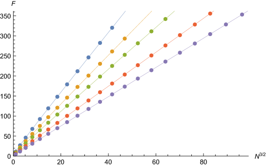
Figure 1: We show the plot of free energy $F=-\log Z_{-}(N,k,M)$ with $M=3$, for $k=3,4,6,8,12$. $k$ increases from the right curve ($k=3$) to the left curve ($k=12$). Note that the horizontal axis is $N^{3/2}$. The dots are the exact values of free energy at integer $N$, while the solid curves represent the perturbative free energy given by the Airy function (20) with $C,B$ in (37) and $A$ in (38).

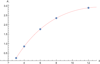
Figure 2: This is the plot of $A_{-}(k,M=3)$ as a function of $k$. The dots are the numerical values of $A_{-}(k,3)$ for $k=3,4,6,8,12$ computed from (41), while the solid curve is the plot of our conjecture of $A_{-}(k,3)$ in (38).

In Figure 1, we show the plot of free energy $F=-\log Z_{-}(N,k,M)$ as a function of $N$ for $M=3$ with $k=3,4,6,8,12$, as an example. As we can see, the exact values of the free energy exhibit a nice agreement with the perturbative one given by the Airy function (20) if we use the correct coefficients $C,B$ in (37) and $A$ in (38). We find the similar agreement for all other cases.

As discussed in HO1 , we can estimate the numerical values of $A_{\pm}(k,M)$ by

$$A_{\pm}(k,M)\approx\log\left[\frac{Z_{\pm}(N,k,M)}{C_{\pm}(k)^{-\frac{1}{3}}\text{Ai}\Bigl{[}C_{\pm}(k)^{-\frac{1}{3}}(N-B_{\pm}(k,M))\Bigr{]}}\right],\quad(N\gg 1).$$ (41)

In practice, we compute the numerical value of $A_{\pm}(k,M)$ from the exact value of $Z_{\pm}(N_{\text{max}},k,M)$ by setting $N=N_{\text{max}}$ in (41). In Figure 2 we show the plot of $A_{-}(k,M)$ for $M=3$, as an example. One can clearly see a nice agreement between the numerical value of $A_{-}(k,3)$ estimated by using (41) and our conjecture of $A_{-}(k,3)$ in (38). Let us take a closer look at the case of $A_{-}(8,3)$. We have computed the exact values of $Z_{-}(N,8,3)$ up to $N_{\text{max}}=14$, and the numerical estimation (41) with $N=14$ gives

$$A_{-}(8,3)\approx 2.34669920....$$ (42)

On the other hand, our proposal of the exact value (38) is

$$A_{-}(8,3)=-\frac{\zeta(3)}{16\pi^{2}}+\frac{5\log(2)}{8}-2\log\left(\sin\frac{\pi}{8}\right)=2.34669923144...,$$ (43)

which is in good agreement with the numerical estimation (42). The difference between (42) and (43) can be attributed to the instanton corrections. The first instanton correction is of order $e^{-\frac{4\mu}{k}}=e^{-\frac{\mu}{2}}$ for $k=8$ in the grand canonical picture, which in the canonical picture corresponds to the correction of the order

$$\exp\left(-\frac{1}{2}\sqrt{\frac{N_{\text{max}}}{C_{-}(8)}}\right)\approx 6.0\times 10^{-8}.$$ (44)

This is indeed the same order as the difference between (42) and (43).

Once we know the perturbative grand potential, we can continue the above procedure to fix the coefficients in the non-perturbative part $J^{\text{np}}_{\pm}(\mu,k,M)$ using our exact data of partition functions $Z_{\pm}(N,k,M)$. The results are summarized in Appendix B. We find that there are three types of instanton corrections with the weight:

$$\mathcal{O}(e^{-\frac{4\mu}{k}}),\qquad\mathcal{O}(e^{-2\mu}),\qquad\mathcal{O}(e^{-\mu}).$$ (45)

The first two types have direct analogue in the ABJ theory, namely, worldsheet instantons and membrane instantons. On the other hand, the last type in (45) is a new contribution coming from the effect of orientifold projection, which we call “half-instantons”, following Okuyama:2015auc . It is curious to observe that there is no contribution with the half-weight of worldsheet instanton of the order $\mathcal{O}(e^{-2\mu/k})$. Only the half-weight of membrane instantons of order $\mathcal{O}(e^{-\mu})$ appear.

For the cases of $k=2,4,8$, by looking at the coefficients of expansion in Appendix B, one can easily guess the all order resummation of instanton expansion, and find the closed form expression of grand partition function $\Xi_{\pm}(\mu,k,M)$, which we will consider in section 4, 5, and 6. By expanding the closed form expression of $\Xi_{\pm}(\mu,k,M)$ around $e^{\mu}=0$, one can read off the exact values of canonical partition functions $Z_{\pm}(N,k,M)$ up to arbitrarily high $N$, in principle. Therefore, one can “bootstrap” the computation of partition functions for $k=2,4,8$:

$$\text{exact~{}values~{}of}~{}Z_{\pm}(N,k,M)~{}~{}~{}(N\leq N_{\text{max}})$$ (46)

$$\Rightarrow{}{} \text{closed~{}form~{}of}~{}~{}\Xi_{\pm}(\mu,k,M)$$

$$\Rightarrow{}{} \text{exact~{}values~{}of}~{}Z_{\pm}(N,k,M)~{}~{}~{}(N>N_{\text{max}}).$$

For example, we have computed the exact values of $Z_{-}(N,8,3)$ up to $N=20$ from the expansion of the closed form expression of the grand partition function $\Xi_{-}(\mu,8,3)$ in (280). Using the exact value of $Z_{-}(N=20,8,3)$, the numerical estimation of $A_{-}(8,3)$ in (41) gets improved

$$A_{-}(8,3)\approx 2.3466992303...,$$ (47)

which is closer to the exact value (43) than the numerical value in (42) obtained from $Z_{-}(N=14,8,3)$, as expected.

2.3 Relation to $\mathcal{N}=5$ $O(n)\times USp(n^{\prime})$ theory

As discussed in ABJ , by introducing orientifold planes into the brane construction of ABJ theory, we can obtain $\mathcal{N}=5$ Chern-Simons-matter theories with gauge group $O(n)\times USp(n^{\prime})$ ABJ ; Hosomichi:2008jb . Now it is natural to ask whether such $\mathcal{N}=5$ theories are related to the projection of ABJ Fermi gas into even/odd sectors. In a recent paper Honda2 , it is observed that the grand partition function constructed from $\rho_{-}$ of ABJM theory ($M=0$) is equivalent to the grand partition function of $\mathcal{N}=5$ $O(2N+1)_{2k}\times USp(2N)_{-k}$ Chern-Simons-matter theory

$$\Xi_{-}(\mu,k,0)=\Xi_{\mathcal{N}=5~{}O(2N+1)_{2k}\times USp(2N)_{-k}}(\mu).$$ (48)

Also, a Fermi gas formalism of $\mathcal{N}=5$ theory with different gauge group $O(2N)_{2k}\times USp(2N)_{-k}$ is studied in MS . We find that the exact values of the canonical partition functions in Table.1 of MS all coincide with the canonical partition functions $Z_{+}(N,k,1)$ computed from the density matrix $\rho_{+}$ of orientifold ABJ theory with $M=1$. From this non-trivial agreement of the canonical partition functions at small $N$, we conjecture that the grand partition functions of these two theories are actually equivalent

$$\Xi_{+}(\mu,k,1)=\Xi_{\mathcal{N}=5~{}O(2N)_{2k}\times USp(2N)_{-k}}(\mu).$$ (49)

It would be interesting to find a direct proof of this equality.

3 WKB expansion

In this section, we will consider the small $k$ expansion (WKB expansion) of the grand potential $J_{\pm}(\mu,k,M)$ of orientifold ABJ theory. As discussed in Okuyama:2015auc , the total grand potential can be written as

$$J_{\pm}(\mu,k,M)=\frac{J(\mu,k,M)\pm J^{R}(\mu,k,M)}{2},$$ (50)

where

$$J(\mu,k,M)=\sum_{\ell=1}^{\infty}\frac{(-1)^{\ell-1}e^{\ell\mu}}{\ell}\operatorname{Tr}(\rho^{\ell}),\quad J^{R}(\mu,k,M)=\sum_{\ell=1}^{\infty}\frac{(-1)^{\ell-1}e^{\ell\mu}}{\ell}\operatorname{Tr}(\rho^{\ell}R),$$ (51)

with $\rho$ being the density matrix of ABJ theory. As we will see in the next section, at the level of modified grand potential (50) does not hold in general. In particular, the sum of $J_{+}$ and $J_{-}$ does not agree with the modified grand potential of ABJ theory

$$J_{+}(\mu,k,M)+J_{-}(\mu,k,M)\not=J(\mu,k,M).$$ (53)

On the other hand, we find that the difference $J_{+}-J_{-}$ is always equal to $J^{R}$ in the examples listed in Appendix B. We should stress that the total grand grand partition function is completely factorized and the total grand potentials satisfy

$$\log\Xi_{+}(\mu,k,M)+\log\Xi_{-}(\mu,k,M)=\log\Xi(\mu,k,M).$$ (54)

The difference in (53) comes from rewriting a double sum into a single sum in (5)

$$\sum_{n_{+}\in\mathbb{Z}}e^{J_{+}(\mu+2\pi in_{+},k,M)}\sum_{n_{-}\in\mathbb{Z}}e^{J_{-}(\mu+2\pi in_{-},k,M)}=\sum_{n\in\mathbb{Z}}e^{J(\mu+2\pi in,k,M)}.$$ (55)

For the case of $k=2,4$, we can write down the difference in (53) explicitly using the exact form of grand partition functions, as we will see in section 4 and section 5.

To find the large $\mu$ expansion of $J_{\pm}(\mu,k,M)$, it is useful to rewrite them in the Mellin-Barnes representation Hatsuda-zeta

$$J(\mu,k,M)=-\int_{\gamma}\frac{ds}{2\pi i}\Gamma(s)\Gamma(-s)\operatorname{Tr}(\rho^{s})e^{s\mu},\quad J^{R}(\mu,k,M)=-\int_{\gamma}\frac{ds}{2\pi i}\Gamma(s)\Gamma(-s)\operatorname{Tr}(\rho^{s}R)e^{s\mu}.$$ (56)

The contour $\gamma$ is taken to be parallel to the imaginary $s$-axis with $0<\Re(s)<1$. Picking up the poles at $s=\ell~{}(\ell=1,2,\cdots)$, we recover (51). On the other hand, closing the contour in the direction $\Re(s)\leq 0$ and picking up the poles on the negative real $s$-axis, we can find the large $\mu$ expansion. Thus, the behavior of $J_{\pm}(\mu,k,M)$ is encoded in the analytic properties of the spectral trace $\operatorname{Tr}(\rho^{s})$ and the twisted spectral trace $\operatorname{Tr}(\rho^{s}R)$. In this section, we will consider the WKB expansion of $\operatorname{Tr}(\rho^{s})$ and $\operatorname{Tr}(\rho^{s}R)$, following a similar computation in Okuyama:2015auc .

3.1 The density matrix of local $\mathbb{F}_{0}$

Since the density matrix of ABJ Fermi gas (4) depends on $k$ explicitly, it is not so obvious how can we compute the WKB expansion of (twisted) spectral traces. Also, the expression of density matrix in (4) makes sense only for integer $M$. In Kashaev:2015wia an analytic continuation of $\rho$ to arbitrary $M$ is found using the relation to the mirror curve of local $\mathbb{F}_{0}$ (note that $\mathbb{F}_{0}=\mathbb{P}^{1}\times\mathbb{P}^{1}$). It turns out that we can systematically compute the small $k$ expansion with fixed $b=M/k$.

Let us briefly recall the construction in Kashaev:2015wia . The density matrix of ABJ theory is identified as

$$\rho=O_{\mathbb{F}_{0}}^{-1}$$ (57)

where $O_{\mathbb{F}_{0}}$ is the quantized mirror curve of local $\mathbb{F}_{0}$

$$O_{\mathbb{F}_{0}}=e^{X}+me^{-X}+e^{Y}+e^{-Y},$$ (58)

with

$$X=x+\frac{p}{2},\qquad Y=\frac{p}{2},\qquad[x,p]=i\hbar.$$ (59)

The Planck constant $\hbar$ is related to the Chern-Simons level $k$ by

$$\hbar=2\pi k,$$ (60)

and the mass parameter $m$ in (58) is related to the parameters in the ABJ theory as

$$m=e^{\beta},\qquad\beta=\pi ik\left(1-2b\right).$$ (61)

As shown in Kashaev:2015wia , the inverse operator of $O_{\mathbb{F}_{0}}$ can be written in terms of the quantum dilogarithm $\Phi(x)$ defined by

$$\Phi(x)=\prod_{n=0}^{\infty}\frac{1+e^{x}\mathfrak{q}^{n+\frac{1}{2}}}{1+e^{\frac{2\pi x}{\hbar}}\widetilde{\mathfrak{q}}^{n+\frac{1}{2}}},$$ (62)

with

$$\mathfrak{q}=e^{i\hbar},\qquad\widetilde{\mathfrak{q}}=e^{-\frac{4\pi^{2}i}{\hbar}}.$$ (63)

From (62), the quantum dilogarithm exhibits the following quasi-periodicity

$$\frac{\Phi(x-\frac{i\hbar}{2})}{\Phi(x+\frac{i\hbar}{2})}=1+e^{x},\qquad\frac{\Phi(x-\pi i)}{\Phi(x+\pi i)}=1+e^{\frac{2\pi x}{\hbar}}.$$ (64)

From this property, for the operators $x,p$ obeying $[x,p]=i\hbar$, one can show that

$$\Phi(p)e^{x}\Phi(p)^{-1}=e^{x}+e^{p+x}.$$ (65)

Using this relation (65) repeatedly, one finds

$$e^{\frac{X}{2}}O_{\mathbb{F}_{0}}e^{\frac{X}{2}}-m=\Phi(x)^{-1}\Phi(p)e^{x}\Phi(p)^{-1}\Phi(x)$$ (66)

and

$$\Phi(p)^{-1}\Phi(x)e^{\frac{X}{2}}O_{\mathbb{F}_{0}}e^{\frac{X}{2}}\Phi(x)^{-1}\Phi(p) =m(1+e^{x-\beta})=m\frac{\Phi\left(x-\beta-\frac{i\hbar}{2}\right)}{\Phi\left(x-\beta+\frac{i\hbar}{2}\right)}.$$ (67)

Now, using the quantum pentagon identity

$$\Phi(p)\Phi(x)=\Phi(x)\Phi(x+p)\Phi(p),$$ (68)

the inverse of $O_{\mathbb{F}_{0}}$ is further rewritten as

$$mO_{\mathbb{F}_{0}}^{-1} =e^{\frac{X}{2}}\Phi(x)^{-1}\Phi(p)\frac{\Phi\left(x-\beta+\frac{i\hbar}{2}\right)}{\Phi\left(x-\beta-\frac{i\hbar}{2}\right)}\Phi(p)^{-1}\Phi(x)e^{\frac{X}{2}}$$ (69)

$$=e^{\frac{X}{2}}\Phi(x)^{-1}\Phi\left(x-\beta+\frac{i\hbar}{2}\right)\frac{\Phi\left(x+p-\beta+\frac{i\hbar}{2}\right)}{\Phi\left(x+p-\beta-\frac{i\hbar}{2}\right)}\Phi\left(x-\beta-\frac{i\hbar}{2}\right)^{-1}\Phi(x)e^{\frac{X}{2}}$$

$$=e^{\frac{X}{2}}\Phi(x)^{-1}\Phi\left(x-\beta+\frac{i\hbar}{2}\right)\frac{1}{1+e^{x+p-\beta}}\Phi\left(x-\beta-\frac{i\hbar}{2}\right)^{-1}\Phi(x)e^{\frac{X}{2}}.$$

Finally, after redefining the variables

$$\widehat{p}=x+p-\beta,\quad\widehat{x}=x-\frac{\beta}{2},$$ (70)

we arrive at the following expression of the density matrix $\rho=O^{-1}_{\mathbb{F}_{0}}$ (up to an overall constant and similarity transformation)

$$\rho=e^{\frac{\widehat{x}}{2}}\frac{\Phi(\widehat{x}-\frac{\beta}{2}+\frac{i\hbar}{4})\Phi(\widehat{x}+\frac{\beta}{2}+\frac{i\hbar}{4})}{\Phi(\widehat{x}-\frac{\beta}{2}-\frac{i\hbar}{4})\Phi(\widehat{x}+\frac{\beta}{2}-\frac{i\hbar}{4})}\frac{1}{2\cosh\frac{\widehat{p}}{2}}.$$ (71)

We are interested in the small $\hbar$ expansion of $\rho$. In this case the denominator of (62) can be ignored, since it is non-perturbative in $\hbar$. Then taking the log of (62) we find

$$\log\Phi(x)=\sum_{\ell=1}^{\infty}\frac{(-e^{x})^{\ell}}{\ell(\mathfrak{q}^{\frac{\ell}{2}}-\mathfrak{q}^{-\frac{\ell}{2}})}+\mathcal{O}(e^{-1/\hbar}).$$ (72)

Plugging this into (71) and expanding around $\hbar=0$, the density matrix is rewritten as

$$\rho=\exp\left(\sum_{n=1}^{\infty}\frac{(-1)^{n}(\hbar/2)^{2n}}{(2n)!}E_{2n}(b)\text{Li}_{1-2n}(-e^{\widehat{x}})\right)\frac{1}{2\cosh\frac{\widehat{x}}{2}}\frac{1}{2\cosh\frac{\widehat{p}}{2}},$$ (73)

where $E_{n}(b)$ is the Euler polynomial defined by

$$\frac{2e^{xb}}{e^{x}+1}=\sum_{n=0}^{\infty}\frac{E_{n}(b)}{n!}x^{n}.$$ (74)

When $b=0$, (73) reduces to the density matrix of ABJM theory

$$\rho_{\text{ABJM}}=\frac{1}{2\cosh\frac{\widehat{x}}{2}}\frac{1}{2\cosh\frac{\widehat{p}}{2}},$$ (75)

since $E_{2n}(0)=0~{}(n\geq 1)$.

Now we are ready to perform the WKB expansion (with $b$ fixed) of the spectral trace $\operatorname{Tr}(\rho^{s})$ and the twisted spectral trace $\operatorname{Tr}(\rho^{s}R)$.

3.2 WKB expansion of spectral trace $\operatorname{Tr}\rho^{s}$

Let us first consider the WKB expansion of the spectral trace $\operatorname{Tr}(\rho^{s})$. As discussed in Okuyama:2015auc , this is easily done by using the Wigner transform $\rho_{W}$ of the density matrix $\rho$. In general, the Wigner transform $A_{W}$ of the operator $A$ is defined by

$$A_{W}=\int dye^{\frac{iPy}{\hbar}}\Big{\langle}X-\frac{y}{2}\Big{|}A\Big{|}X+\frac{y}{2}\Big{\rangle}.$$ (76)

Using the property of Wigner transformation

$$(AB)_{W}=A_{W}\star B_{W}\equiv A_{W}e^{\frac{i\hbar}{2}(\overleftarrow{\partial_{X}}\overrightarrow{\partial_{P}}-\overleftarrow{\partial_{P}}\overrightarrow{\partial_{X}})}B_{W},$$ (77)

$$f(\widehat{x})_{W}=f(X),\qquad g(\widehat{p})_{W}=g(P),$$

we find that the Wigner transform of the density matrix $\rho$ (73) is given by

$$\rho_{W}=\exp\left(\sum_{n=1}^{\infty}\frac{(-1)^{n}(\hbar/2)^{2n}}{(2n)!}E_{2n}(b)\text{Li}_{1-2n}(-e^{X})\right)\frac{1}{2\cosh\frac{X}{2}}\star\frac{1}{2\cosh\frac{P}{2}}.$$ (78)

From (77), the Wigner transform of the $\ell^{\text{th}}$ power of $\rho$ is easily obtained by the star-product of $\rho_{W}$’s

$$(\rho^{\ell})_{W}=\underbrace{\rho_{W}\star\cdots\star\rho_{W}}_{\ell}.$$ (79)

The WKB expansion of $(\rho^{\ell})_{W}$ can be computed recursively from the obvious relation $(\rho^{\ell})_{W}=\rho_{W}\star(\rho^{\ell-1})_{W}$. Finally, the WKB expansion of trace $\operatorname{Tr}(\rho^{\ell})$ can be found by integrating $(\rho^{\ell})_{W}$ on the classical phase space

$$\operatorname{Tr}(\rho^{\ell})=\int\frac{dXdP}{2\pi\hbar}(\rho^{\ell})_{W}.$$ (80)

As discussed in Hatsuda-zeta , the WKB expansion of the spectral trace $\operatorname{Tr}(\rho^{s})$ takes the following form

$$\operatorname{Tr}(\rho^{s})=Z_{0}(s)\left(1+\sum_{n=1}^{\infty}D_{n}(s)\hbar^{2n}\right).$$ (81)

The leading term is simply given by

$$Z_{0}(s)=\int\frac{dXdP}{2\pi\hbar}\left(\frac{1}{2\cosh\frac{X}{2}}\frac{1}{2\cosh\frac{P}{2}}\right)^{s}=\frac{1}{2\pi\hbar}\frac{\Gamma(s/2)^{4}}{\Gamma(s)^{2}}.$$ (82)

The correction terms $D_{n}(s)$ can be systematically computed by making an ansatz that $D_{n}(s)$ is a rational function of $s$ and fixing the coefficients in the ansatz by matching the values at integer $s$ Hatsuda-zeta ; Okuyama:2015auc . In this way, we have computed $D_{n}(s)$ up to $n=10$. The first three terms are

$$D_{1}(s) =\frac{-s^{3}-12s^{2}\left(b-b^{2}\right)+s^{2}}{384(s+1)},$$ (83)

$$D_{2}(s) =\frac{s^{3}}{1474560(s+1)(s+3)}\Big{[}7s^{3}-20s^{2}(6b^{2}-6b-1),$$

$$\qquad+s(720b^{4}-1440b^{3}+360b^{2}+360b-11)+16(120b^{4}-240b^{3}+120b^{2}-1)\Big{]}$$

$$D_{3}(s) =-\frac{s^{3}}{3963617280(s+1)(s+3)(s+5)}\Big{[}31s^{6}-3\left(196b^{2}-196b-115\right)s^{5}$$

$$\quad+\left(5040b^{4}-10080b^{3}-1344b^{2}+6384b+1273\right)s^{4}$$

$$\quad+\left(-20160b^{6}+60480b^{5}-11760b^{4}-77280b^{3}+24780b^{2}+23940b+1567\right)s^{3}$$

$$\quad-16\left(10080b^{6}-30240b^{5}+21000b^{4}+8400b^{3}-6804b^{2}-2436b+41\right)s^{2}$$

$$\quad-768\left(448b^{6}-1344b^{5}+1120b^{4}-189b^{2}-35b+3\right)s$$

$$\quad-256\left(672b^{6}-2016b^{5}+1680b^{4}-336b^{2}+1\right)\Big{]}.$$

Then, the WKB expansion of grand potential can be found by acting the differential operator on the leading term

$$J(\mu,k,M)=\left(1+\sum_{n=1}^{\infty}D_{n}(\partial_{\mu})\hbar^{2n}\right)J_{0}(\mu,k,M),$$ (84)

where the leading term $J_{0}(\mu,k,M)$ is given by

$$J_{0}(\mu,k,M)=-\int_{\gamma}\frac{ds}{2\pi i}\Gamma(s)\Gamma(-s)Z_{0}(s)e^{s\mu}.$$ (85)

The perturbative part comes from the pole at $s=0$

$$J_{0}^{\text{pert}}(\mu,k,M)=-\oint_{s=0}\frac{ds}{2\pi i}\Gamma(s)\Gamma(-s)Z_{0}(s)e^{s\mu}=\frac{2}{3\pi^{2}k}\mu^{3}+\frac{1}{3k}\mu+\frac{2\zeta(3)}{\pi^{2}k}.$$ (86)

To find the $\hbar$ corrections to the perturbative grand potential, it is sufficient to expand $D_{n}(s)$ up to $s^{3}$, since $J_{0}^{\text{pert}}(\mu,k,M)$ is a cubic polynomial in $\mu$. In the small $s$ expansion, we find that $D_{n}(s)$ behaves as

$$D_{n}(s) =\frac{1-12b+12b^{2}}{384}s^{2}\delta_{n,1}$$ (87)

$$+\frac{(-1)^{n}s^{3}}{16(2n)!}\Big{[}4^{1-n}B_{2n-2}B_{2n}+B_{2n-2}(B_{2n}(b)-B_{2n})\Big{]}+\mathcal{O}(s^{4}).$$

Here $B_{2n}(b)$ and $B_{2n}=B_{2n}(0)$ denote the Bernoulli polynomial and the Bernoulli number, respectively. By acting the differential operator (84) on (86), we find that the constant $C(k)$ and $B(k,M)$ in (13) are correctly reproduced. For instance, the $\mu$-linear term in $J^{\text{pert}}$ becomes

$$\frac{1}{3k}\mu+\hbar^{2}\frac{1-12b+12b^{2}}{384}\partial_{\mu}^{2}\left(\frac{2\mu^{3}}{3\pi^{2}k}\right)=\left[\frac{1}{3k}-\frac{k}{12}+\frac{k}{2}\left(\frac{1}{2}-b\right)^{2}\right]\mu,$$ (88)

which correctly reproduces $B(k,M)$ in (13). Also, we can read off the WKB expansion of constant term $A(k,M)$

$$A(k,M) =\frac{2\zeta(3)}{\pi^{2}k}+\frac{1}{2\pi\hbar}\sum_{n=1}^{\infty}\frac{4^{1-n}(-1)^{n}B_{2n-2}B_{2n}\hbar^{2n}}{(2n)!}$$ (89)

$$\qquad+\frac{1}{2\pi\hbar}\sum_{n=1}^{\infty}\frac{(-1)^{n}B_{2n-2}(B_{2n}(b)-B_{2n})\hbar^{2n}}{(2n)!}.$$

The first line of (89) agrees with the constant term in ABJM theory KEK

$$A_{c}(k)=\frac{2\zeta(3)}{\pi^{2}k}+\sum_{n=1}^{\infty}\frac{(-1)^{n}B_{2n-2}B_{2n}\pi^{2n-2}k^{2n-1}}{(2n)!}.$$ (90)

As we will see below, the second line in (89) corresponds to the WKB expansion of the free energy $F_{\text{coni}}(k,M)$ of the $U(M)_{k}$ pure Chern-Simons theory. To see this, let us consider the WKB expansion of $F_{\text{coni}}(k,M)$. In terms of $\hbar=2\pi k$ (60), $F_{\text{coni}}(k,M)$ in (17) is rewritten as

$$F_{\text{coni}}(k,M)=-\left(\frac{\hbar}{4\pi^{2}}\right)^{2}F_{0}(b)+\frac{\hbar}{4\pi^{2}}\int_{0}^{\infty}dy\frac{\hbar y}{e^{\hbar y}-1}\log\left(\frac{\cosh 2\pi y-\cos 2\pi b}{\cosh 2\pi y-1}\right).$$ (91)

By expanding the integrand in $\hbar$

$$\frac{\hbar y}{e^{\hbar y}-1}=1-\frac{\hbar y}{2}+\sum_{n=2}^{\infty}\frac{B_{2n-2}}{(2n-2)!}(\hbar y)^{2n-2},$$ (92)

and making use of the identities

$$\int_{0}^{\infty}dyy\log\left(\frac{\cosh 2\pi y-\cos 2\pi b}{\cosh 2\pi y-1}\right) =-\frac{1}{2\pi^{2}}F_{0}(b),$$ (93)

$$\int_{0}^{\infty}\frac{dy}{2\pi}y^{2n-2}\log\left(\frac{\cosh 2\pi y-\cos 2\pi b}{\cosh 2\pi y-1}\right) =\frac{(-1)^{n}(B_{2n}(b)-B_{2n})}{2n(2n-1)},\quad(n\geq 2),$$

one can see that the small $\hbar$ expansion of $F_{\text{coni}}(k,M)$ indeed agrees with the second line of (89). To summarize, the perturbative grand potential of ABJ theory with the coefficients $C(k),B(k,M)$ in (13) and $A(k,M)$ in (14) are correctly reproduced from the WKB expansion of the spectral trace $\operatorname{Tr}(\rho^{s})$.

3.3 WKB expansion of twisted spectral trace $\operatorname{Tr}(\rho^{s}R)$

In a similar manner as in the previous subsection 3.2, we can compute the WKB expansion of the twisted spectral trace $\operatorname{Tr}(\rho^{s}R)$. This can be done using the fact that $\operatorname{Tr}(AR)$ for some operator $A$ is easily obtained from its Wigner transform $A_{W}$ by simply setting $X=P=0$ Okuyama:2015auc

$$\operatorname{Tr}(AR)=\frac{1}{2}A_{W}\Big{|}_{X=P=0}.$$ (94)

We find that the WKB expansion of $\operatorname{Tr}(\rho^{s}R)$ is written as

$$\operatorname{Tr}(\rho^{s}R)=Z_{0}^{R}(s)\left(1+\sum_{n=1}^{\infty}D_{n}^{R}(s)\hbar^{2n}\right).$$ (95)

The leading term is given by

$$Z_{0}^{R}(s)=2^{-1-2s}.$$ (96)

We have computed the correction terms $D_{n}^{R}(s)$ up to $n=12$. The first three terms are given by

$$D_{1}^{R}(s) =-\frac{s^{2}}{128}+\frac{1}{32}s(b-1)b,$$ (97)

$$D_{2}^{R}(s) =\frac{5s^{4}}{98304}+\frac{s^{3}\left(-2b^{2}+2b+1\right)}{8192}+\frac{s^{2}\left(6b^{4}-12b^{3}+6b+1\right)}{12288}+\frac{s\left(b^{4}-2b^{3}+b\right)}{3072},$$

$$D_{3}^{R}(s) =-\frac{61s^{6}}{188743680}+\frac{\left(5b^{2}-5b-7\right)s^{5}}{3145728}+\frac{\left(-18b^{4}+36b^{3}+30b^{2}-48b-29\right)s^{4}}{4718592}$$

$$\quad+\frac{\left(2b^{6}-6b^{5}-b^{4}+12b^{3}+4b^{2}-11b-3\right)s^{3}}{393216}+\frac{\left(6b^{6}-18b^{5}+30b^{3}+3b^{2}-21b-2\right)s^{2}}{589824}$$

$$\quad+\frac{b\left(b^{5}-3b^{4}+5b^{2}-3\right)s}{184320}.$$

Again, the large $\mu$ expansion of $J^{R}(\mu,k,M)$ is found by acting differential operators on the leading term

$$J^{R}(\mu,k,M)=\left(1+\sum_{n=1}^{\infty}D_{n}^{R}(\partial_{\mu})\hbar^{2n}\right)J_{0}^{R}(\mu,k,M),$$ (98)

where the leading term $J_{0}^{R}(\mu,k,M)$ is given by

$$J_{0}^{R}(\mu,k,M)=-\int_{\gamma}\frac{ds}{2\pi i}\Gamma(s)\Gamma(-s)Z_{0}^{R}(s)e^{s\mu}.$$ (99)

Perturbative part.

Let us first consider the perturbative part of $J^{R}(\mu,k,M)$, which comes from the pole at $s=0$. The leading term is give by

$$\frac{1}{2}J_{0}^{R,\text{pert}}(\mu,k,M)=-\frac{1}{2}\oint_{s=0}\frac{ds}{2\pi i}\Gamma(s)\Gamma(-s)Z_{0}^{R}(s)e^{s\mu}=\frac{\mu}{4}-\frac{1}{2}\log 2.$$ (100)

This is consistent with the $\pm 1/4$ shift of $B_{\pm}(k,M)$ in (37). As in the previous subsection 3.2, the contribution $F_{\text{non-ori}}$ in (38) is obtained by summing all order corrections in $\hbar$. Since (100) is a linear function in $\mu$, in order to compute the term $F_{\text{non-ori}}$ it is sufficient to expand $D_{n}^{R}(s)$ up to the linear order in $s$. We find that $D_{n}^{R}(s)$ behaves as

$$D_{n}^{R}(s)=\frac{1}{2}\frac{(-1)^{n}E_{2n-1}(0)E_{2n}(b)}{(2n)!2^{2n}}s+\mathcal{O}(s^{2}).$$ (101)

As we will see below, this indeed reproduces the WKB expansion of $F_{\text{non-ori}}$ in (40). By integration by parts and rescaling of integral variable, (40) is rewritten as

$$F_{\text{non-ori}}=\frac{\hbar}{8\pi^{2}}\text{Im}\Big{[}\text{Li}_{2}(e^{-i\pi b})-\text{Li}_{2}(-e^{-i\pi b})\Big{]}+\frac{1}{4}\log 2-\int_{0}^{\infty}dx\log(1+e^{-\frac{\hbar x}{2}})\frac{\sin\pi b\cosh\pi x}{\cosh 2\pi x-\cos 2\pi b}.$$ (102)

By expanding the integrand $\log(1+e^{-\frac{\hbar x}{2}})$ in small $\hbar$

$$\log(1+e^{-\frac{\hbar x}{2}})=\log 2-\frac{\hbar x}{4}-\frac{1}{2}\sum_{n=1}^{\infty}\frac{E_{2n-1}(0)}{(2n)!}\Bigl{(}\frac{\hbar x}{2}\Bigr{)}^{2n},$$ (103)

and using the formula

$$\int_{0}^{\infty}dx\frac{x^{2n}\sin\pi b\cosh\pi x}{\cosh 2\pi x-\cos 2\pi b} =\frac{(-1)^{n}}{4}E_{2n}(b),\quad(n\geq 0),$$ (104)

$$\int_{0}^{\infty}dx\frac{x\sin\pi b\cosh\pi x}{\cosh 2\pi x-\cos 2\pi b} =-\frac{1}{2\pi^{2}}\text{Im}\Big{[}\text{Li}_{2}(e^{-i\pi b})-\text{Li}_{2}(-e^{-i\pi b})\Big{]},$$

the small $\hbar$ expansion of $F_{\text{non-ori}}$ with fixed $b$ is found to be

$$F_{\text{non-ori}}=\frac{1}{8}\sum_{n=1}^{\infty}\frac{(-1)^{n}E_{2n-1}(0)E_{2n}(b)}{(2n)!2^{2n}}\hbar^{2n}.$$ (105)

We can compare this with the WKB expansion of twisted spectral trace in (101). By acting the differential operator $D_{n}(\partial_{\mu})$ (101) on the leading term $J_{0}^{R,\text{pert}}$ in (100), one can easily show that the constant term of the perturbative part of $\frac{1}{2}J^{R}$ agrees with the WKB expansion of $F_{\text{non-ori}}$ in (105)

$$\frac{1}{2}J^{R,\text{pert}}=\frac{1}{2}\left(1+\sum_{n=1}^{\infty}D_{n}^{R}(\partial_{\mu})\hbar^{2n}\right)J_{0}^{R,\text{pert}}=\frac{\mu}{4}-\frac{1}{2}\log 2+F_{\text{non-ori}}.$$ (106)

This correctly reproduces the shift in $A_{\pm}(k,M)$ in (38).

Instanton corrections.

$J^{R}(\mu,k,M)$ can be written as a sum of the perturbative part and instanton corrections

$$J^{R}(\mu,k,M)=J^{R,\text{pert}}(\mu,k,M)+J^{R,\text{np}}(\mu,k,M).$$ (107)

By picking up the poles at negative integers $s=-\ell~{}(\ell=1,2,\cdots)$ in (99), we can compute the non-perturbative correction $J^{R,\text{np}}(\mu,k,M)$, which we identify as the “half-instanton” corrections in (45). From (98) and (99), one can show that the instanton corrections are given by

$$J^{R,\text{np}}(\mu,k,M) =\sum_{\ell=1}^{\infty}r_{\ell}(\hbar,b)e^{-\ell\mu},$$ (108)

$$r_{\ell}(\hbar,b) =\left(1+\sum_{n=1}^{\infty}D_{n}^{R}(-\ell)\hbar^{2n}\right)\frac{(-1)^{\ell-1}2^{-1+2\ell}}{\ell}.$$

By matching the WKB expansion, we find the first few instanton coefficients $r_{\ell}(\hbar,b)$ in closed forms

$$r_{1}(\hbar,b) =2\cos\theta_{b},$$ (109)

$$r_{2}(\hbar,b) =-2(\cos 2\theta_{b}+\cos 2\theta_{0}),$$

$$r_{3}(\hbar,b) =\frac{4}{3}(\cos 3\theta_{b}+3\cos\theta_{b}\cos^{2}2\theta_{0}),$$

$$r_{4}(\hbar,b) =-4(\cos 4\theta_{b}+4\cos 2\theta_{b}\cos^{3}2\theta_{0}+\cos^{2}4\theta_{0}+2\cos^{2}2\theta_{0}),$$

$$r_{5}(\hbar,b) =\frac{32}{5}(\cos 5\theta_{b}+5\cos 3\theta_{b}\cos^{4}2\theta_{0}+5\cos\theta_{b}\cos^{2}2\theta_{0}(1+\cos^{2}4\theta_{0})),$$

$$r_{6}(\hbar,b) =-\frac{32}{3}\Bigl{(}\cos 6\theta_{b}+6\cos 4\theta_{b}\cos^{5}2\theta_{0}+3\cos 2\theta_{b}\frac{\cos^{5}4\theta_{0}-1}{\cos 4\theta_{0}-1}$$

$$\qquad+\cos^{3}2\theta_{0}(6\cos^{3}4\theta_{0}-3\cos^{2}4\theta_{0}+3\cos 4\theta_{0}+4)\Bigr{)},$$

$$r_{7}(\hbar,b) =\frac{128}{7}\Bigl{(}\cos 7\theta_{b}+7\cos 5\theta_{b}\cos^{6}2\theta_{0}+7\cos 3\theta_{b}\cos^{2}2\theta_{0}(\cos^{2}4\theta_{0}+2\cos^{2}2\theta_{0})(\cos^{2}4\theta_{0}+2\sin^{2}2\theta_{0})$$

$$\qquad+7\cos\theta_{b}\cos^{4}2\theta_{0}(4\cos^{4}4\theta_{0}-4\cos^{3}4\theta_{0}+3\cos^{2}4\theta_{0}+2)\Bigr{)}.$$

Here we have introduced the notation $\theta_{b}$ and $\theta_{0}$ by

$$\theta_{b}=\frac{\hbar(1-2b)}{8},\qquad\theta_{0}=\frac{\hbar}{8}.$$ (110)

When $k$ and $M$ are both integers, $r_{\ell}(\hbar,b)$ becomes simpler and we can easily guess the instanton coefficients $r_{\ell}(\hbar,b)$ for all order in $\ell$. From (110) and the periodicity of trigonometric functions, the result depends on the value of $k$ modulo 8. For odd $M$ we find

$$J^{R,\text{np}}(k\equiv 1,3~{}\text{mod}8)=-J^{R,\text{np}}(k\equiv 5,7~{}\text{mod}8) =\frac{1}{4}\log\left(\frac{1+2\sqrt{2}(-1)^{\frac{M-1}{2}}e^{-\mu}+4e^{-2\mu}}{1-2\sqrt{2}(-1)^{\frac{M-1}{2}}e^{-\mu}+4e^{-2\mu}}\right),$$ (111)

$$J^{R,\text{np}}(k\equiv 2~{}\text{mod}8)=-J^{R,\text{np}}(k\equiv 6~{}\text{mod}8) =\frac{1}{4}\log\frac{1+4(-1)^{\frac{M-1}{2}}e^{-\mu}}{1-4(-1)^{\frac{M-1}{2}}e^{-\mu}},$$

$$J^{R,\text{np}}(k\equiv 0,4~{}\text{mod}8) =0,$$

while for even $M$ we find

$$J^{R,\text{np}}(k\equiv 1,7~{}\text{mod}8)=-J^{R,\text{np}}(k\equiv 3,5~{}\text{mod}8) =\frac{1}{4}\log\left(\frac{1+2\sqrt{2}(-1)^{\frac{M}{2}}e^{-\mu}+4e^{-2\mu}}{1-2\sqrt{2}(-1)^{\frac{M}{2}}e^{-\mu}+4e^{-2\mu}}\right),$$ (112)

$$J^{R,\text{np}}(k\equiv 2,6~{}\text{mod}8) =\frac{1}{4}\log(1+16e^{-2\mu}),$$

$$J^{R,\text{np}}(k\equiv 0~{}\text{mod}8) =\frac{1}{2}\log(1+4(-1)^{\frac{M}{2}}e^{-\mu}),$$

$$J^{R,\text{np}}(k\equiv 4~{}\text{mod}8) =\frac{1}{2}\log(1-4(-1)^{\frac{M}{2}}e^{-\mu}).$$

For $M=1$, (111) reproduces the results of half-instantons in $\mathcal{N}=5$ $O(2N)_{2k}\times USp(2N)_{-k}$ theory found in MS . Also, for all cases in Appendix B with various integral $k$ and $M$, the difference between the modified grand potentials $J_{+}$ and $J_{-}$ agrees with the results in (111) and (112)

$$J_{+}^{\text{np}}(\mu,k,M)-J_{-}^{\text{np}}(\mu,k,M)=J^{R,\text{np}}(\mu,k,M).$$ (113)

4 Exact grand partition functions for $k=2$

In this section, we will write down the exact grand partition functions of orientifold ABJ theory $\Xi_{\pm}(\mu,k,M)$ for $k=2$ with $M=0,1$. In general, in order to find the exact grand partition function, first we need to find the closed form expression of the modified grand potential. Then, by performing the periodic sum (5), we can construct the grand partition function. It turns out that for $k=2$ the modified grand potential is determined by the genus-zero and genus-one free energies of topological string, and the exact grand partition function is written in terms of Jacobi theta functions, as in CGM ; GHM . The genus-zero free energy of ABJ(M) theory is encoded in the classical periods of local $\mathbb{P}^{1}\times\mathbb{P}^{1}$, which we review first in the next subsection. Then we proceed to write down the exact grand partition functions of orientifold ABJ theory for $k=2$.

4.1 Periods of diagonal local $\mathbb{P}^{1}\times\mathbb{P}^{1}$

In this subsection, we summarize the known results of classical periods of the spectral curve of ABJM matrix model, or the mirror curve of diagonal local $\mathbb{P}^{1}\times\mathbb{P}^{1}$ DMP ; GHM . The spectral curve of ABJM matrix model has genus one, hence there are two independent periods: A-period and B-period. These two periods are characterized by the Picard-Fuchs equation

$$[\theta^{3}-4z\theta(2\theta+1)^{2}]\Pi=0,$$ (114)

where

$$\theta=z\partial_{z},\quad z=e^{-2\mu}.$$ (115)

To study the small $z$ expansion and the large $z$ expansion of periods systematically, it is useful to write the solution of (114) in a Mellin-Barnes type integral representation. By plugging the ansatz

$$\Pi=\int\frac{ds}{2\pi i}f(s)z^{s},$$ (116)

into (114), we find that $f(s)$ should satisfy

$$s^{3}f(s)-2f(s-1)\frac{\Gamma(2s)^{2}}{\Gamma(2s-2)\Gamma(2s-1)}=0.$$ (117)

One can easily find two independent solutions:

$$f_{A}(s)=-\frac{4s\Gamma(-s)\Gamma(2s)^{2}}{\Gamma(s+1)^{3}},\quad f_{B}(s)=-\frac{\Gamma(-s)^{3}\Gamma(2s)}{\Gamma(s+1)\Gamma(-2s)}.$$ (118)

In the large radius frame (small $z$ region), these two solutions correspond to the flat coordinate $t$ (A-period) and the derivative of the genus-zero free energy (B-period)

$$\int_{\gamma^{\prime}}\frac{ds}{2\pi i}f_{A}(s)z^{s}=t,\qquad\int_{\gamma^{\prime}}\frac{ds}{2\pi i}f_{B}(s)z^{s}=\partial_{t}F_{0}+\frac{\pi^{2}}{6},$$ (119)

where the integration contour $\gamma^{\prime}$ is taken to be parallel to the imaginary $s$-axis with $-1/2<\Re(s)<0$. The small $z$ expansion of those periods are easily obtained by picking up the poles at $s=0,1,2,\cdots$,

$$t =-\sum_{n=0}^{\infty}\text{Res}_{s=n}\Big{[}f_{A}(s)z^{s}\Big{]}=-\log z+w_{a},$$ (120)

$$\partial_{t}F_{0}+\frac{\pi^{2}}{6} =-\sum_{n=0}^{\infty}\text{Res}_{s=n}\Big{[}f_{B}(s)z^{s}\Big{]}=\frac{1}{2}(t^{2}-w_{a}^{2}+w_{b}).$$

Note that the constant $\pi^{2}/6$ in the B-period comes from the pole at $s=0$

$$-\text{Res}_{s=0}\Big{[}f_{B}(s)z^{s}\Big{]}=\frac{1}{2}(\log z)^{2}+\frac{\pi^{2}}{6}.$$ (121)

$w_{a}$ and $w_{b}$ in (120) are given by

$$w_{a} =-\sum_{n=1}^{\infty}\frac{1}{n}\left(\frac{\Gamma(n+\frac{1}{2})}{\Gamma(\frac{1}{2})n!}\right)^{2}(-16z)^{n},$$ (122)

$$w_{b} =\sum_{n=1}^{\infty}\frac{8}{n}\left(\frac{\Gamma(n+\frac{1}{2})}{\Gamma(\frac{1}{2})n!}\right)^{2}\left[\psi(2n)-\psi(n)-\frac{3}{4n}\right](-16z)^{n},$$

where $\psi(n)$ denotes the digamma function. The A-period and the B-period in (120) can be written in closed forms in terms of a hypergeometric function and a Meijer $G$-function, respectively

$$t =-\log z+4z{}_{4}F_{3}\left(1,1,\frac{3}{2},\frac{3}{2};2,2,2;-16z\right),$$ (123)

$$\partial_{t}F_{0}+\frac{\pi^{2}}{6} =\frac{1}{\pi}G^{3,2}_{3,3}\left(\begin{matrix}\frac{1}{2},&\frac{1}{2},&1\\ 0,&0,&0\end{matrix}\Big{|}-16z\right)+\pi it.$$

From these relations, one can find the genus-zero free energy $F_{0}(t)$ as a function of $t$. The integration constant in $F_{0}(t)$ is found to be $-2\zeta(3)$, and the large $t$ expansion of $F_{0}(t)$ is given by

$$F_{0}(t)=\frac{t^{3}}{6}-2\zeta(3)+4e^{-t}-\frac{9}{2}e^{-2t}+\frac{328}{27}e^{-3t}-\frac{777}{16}e^{-4t}+\frac{30004}{125}e^{-5t}+\cdots.$$ (124)

It turns out that the logarithmic derivatives of $t$ and $\partial_{t}F_{0}$ with respect to $z$ are simpler than $t$ and $\partial_{t}F_{0}$ themselves, and they are given by the complete elliptic integral of the first kind

$$-z\partial_{z}t =\frac{2}{\pi}K(-16z),$$ (125)

$$-z\partial_{z}\partial_{t}F_{0}(t) =2K(1+16z)+2iK(-16z).$$

Taking the ratio of them, we find the modulus of the spectral curve

$$\tau_{L}=\frac{i}{\pi}\partial_{t}^{2}F_{0}(t)=i\frac{K(1+16z)}{K(-16z)}-1.$$ (126)

Here the subscript $L$ stands for the “large radius frame”.

On the other hand, by deforming the contour $\gamma^{\prime}$ of (119) in the direction $\Re(s)<0$ and picking up the poles at $s=-(n+1/2),~{}(n=0,1,2,\cdots)$, we find the small $\kappa$ expansion of the periods, where $\kappa$ is defined by

$$\kappa=e^{\mu},\quad z=\kappa^{-2}.$$ (127)

Then the two periods in (119) become

$$\int\frac{ds}{2\pi i}f_{A}(s)z^{s} =\sum_{n=0}^{\infty}\text{Res}_{s=-(n+1/2)}\Big{[}f_{A}(s)\kappa^{-2s}\Big{]}=\frac{1}{\pi^{2}}\partial_{\lambda}\mathcal{F}_{0},$$ (128)

$$\int\frac{ds}{2\pi i}f_{B}(s)z^{s} =\sum_{n=0}^{\infty}\text{Res}_{s=-(n+1/2)}\Big{[}f_{B}(s)\kappa^{-2s}\Big{]}=4\pi^{2}\lambda.$$

By performing the sum of residues in (128), we find that the flat coordinate $\lambda$ and the genus-zero free energy $\mathcal{F}_{0}(\lambda)$ in the “orbifold frame” are given by

$$\lambda =\frac{\kappa}{8\pi}{}_{3}F_{2}\left(\frac{1}{2},\frac{1}{2},\frac{1}{2};1,\frac{3}{2};-\frac{\kappa^{2}}{16}\right),$$ (129)

$$\partial_{\lambda}\mathcal{F}_{0} =\frac{\kappa}{4}G^{2,3}_{3,3}\left(\begin{matrix}\frac{1}{2},&\frac{1}{2},&\frac{1}{2}\\ 0,&0,&-\frac{1}{2}\end{matrix}\Big{|}-\frac{\kappa^{2}}{16}\right)+4\pi^{3}i\lambda.$$

The small $\lambda$ expansion of the free energy $\mathcal{F}_{0}(\lambda)$ reads

$$\mathcal{F}_{0}(\lambda)=2\pi^{2}\lambda^{2}\left(3-2\log\frac{\pi\lambda}{2}\right)+\frac{4\pi^{4}\lambda^{4}}{9}+\cdots.$$ (130)

In this case, the ordinary derivatives of $\lambda$ and $\partial_{\lambda}\mathcal{F}_{0}$ with respect to $\kappa$ become the complete elliptic integral

$$8\pi\partial_{\kappa}\lambda =\frac{2}{\pi}K\Bigl{(}-\frac{\kappa^{2}}{16}\Bigr{)},$$ (131)

$$\partial_{\kappa}\partial_{\lambda}\mathcal{F}_{0} =\pi K\Bigl{(}1+\frac{\kappa^{2}}{16}\Bigr{)}+\pi iK\Bigl{(}-\frac{\kappa^{2}}{16}\Bigr{)},$$

and the torus modulus in the orbifold frame is given by

$$\tau_{\text{orb}}=\frac{i}{4\pi^{3}}\partial_{\lambda}^{2}\mathcal{F}_{0}=i\frac{K\Bigl{(}1+\frac{\kappa^{2}}{16}\Bigr{)}}{K\Bigl{(}-\frac{\kappa^{2}}{16}\Bigr{)}}-1.$$ (132)

As we will see below, the difference of the derivatives between (125) and (131) plays an important role in the modular covariance of the grand partition functions.

Since (119) and (128) are just the different expansions of the same integrals, they are related by

$$t=\frac{\partial_{\lambda}\mathcal{F}_{0}}{\pi^{2}},\qquad\partial_{t}F_{0}+\frac{\pi^{2}}{6}=4\pi^{2}\lambda.$$ (133)

In other words, the role of A-cycle and B-cycle are essentially exchanged when going from the large radius frame to the orbifold frame. In fact, $\tau_{L}$ (126) and $\tau_{\text{orb}}$ (132) are related by the $S$-transformation

$$\tau_{\text{orb}}=-\frac{1}{\tau_{L}}.$$ (134)

Finally, the genus-zero free energy of the large radius frame $F_{0}$ and the orbifold frame $\mathcal{F}_{0}$ are related by

$$F_{0}+\frac{\pi^{2}t}{6}=\int d\kappa\partial_{\kappa}t\left(\partial_{t}F_{0}+\frac{\pi^{2}}{6}\right)=\int d\kappa\frac{\partial_{\kappa}\partial_{\lambda}\mathcal{F}_{0}}{\pi^{2}}\cdot 4\pi^{2}\lambda=-4(\mathcal{F}_{0}-\lambda\partial_{\lambda}\mathcal{F}_{0}).$$ (135)

4.2 The case of $(k,M)=(2,0)$

In this subsection, we write down the closed form expression of the grand partition functions $\Xi_{\pm}(\mu,2,0)$ of orientifold ABJ theory. As in CGM ; GHM , we find that $\Xi_{\pm}(\mu,2,0)$ are written in terms of the Jacobi theta functions. Also, they have a nice property under modular transformation, which enables us to find the expansion around the orbifold point $\kappa\to 0$ and extract the canonical partition function at fixed $N$.

4.2.1 $\Xi(\mu,2,0)$

Let us recall the grand partition function $\Xi(\mu,2,0)$ of ABJM theory CGM before projection to $R=\pm 1$. In CGM , it was found that the modified grand potential is essentially determined by the genus-zero and genus-one data of the (refined) topological string on local $\mathbb{P}^{1}\times\mathbb{P}^{1}$. The large $\mu$ expansion of the modified grand potential is given by HMO2

$$J(\mu,2,0) =\frac{\mu^{3}}{3\pi^{2}}+\frac{\mu}{4}-\frac{\zeta(3)}{2\pi^{2}}$$ (136)

$$+\left[\frac{4\mu^{2}+2\mu+1}{\pi^{2}}\right]e^{-2\mu}+\left[-\frac{52\mu^{2}+\mu+9/4}{2\pi^{2}}+2\right]e^{-4\mu}$$

$$+\left[\frac{736\mu^{2}-304/3\mu+154/9}{3\pi^{2}}-32\right]e^{-6\mu}$$

$$+\left[-\frac{2701\mu^{2}-13949/24\mu+11291/192}{\pi^{2}}+466\right]e^{-8\mu}+\cdots,$$

where the first line corresponds to the perturbative part, while the remaining terms are instanton corrections. As observed in CGM , the terms with and without $1/\pi^{2}$ coefficient, which we call $f_{0}$ and $f_{1}$, respectively, have different origins. Accordingly, it is natural to decompose the modified grand potential as

$$J(\mu,2,0)=f_{0}+f_{1},$$ (137)

where

$$f_{0} =\frac{\mu^{3}}{3\pi^{2}}-\frac{\zeta(3)}{2\pi^{2}}+\frac{4\mu^{2}+2\mu+1}{\pi^{2}}e^{-2\mu}-\frac{52\mu^{2}+\mu+9/4}{2\pi^{2}}e^{-4\mu}+\cdots,$$ (138)

$$f_{1} =\frac{\mu}{4}+2e^{-4\mu}-32e^{-6\mu}+466e^{-8\mu}+\cdots.$$

It turns out that $f_{0}$ can be written in a closed form in terms of the genus-zero free energy $F_{0}(t)$

$$f_{0}=\frac{1}{4\pi^{2}}\left(F_{0}-t\partial_{t}F_{0}+\frac{t^{2}}{2}\partial_{t}^{2}F_{0}\right).$$ (139)

On the other hand, $f_{1}$ is given by the sum of the genus-one free energies of the standard topological string and the refined topological string in the Nekrasov-Shatashvili limit

$$f_{1}=\frac{\mu}{4}+F_{1}+F_{1}^{\text{NS}}$$ (140)

where the first term comes from the perturbative grand potential. Explicit forms of $F_{1}$ and $F_{1}^{\text{NS}}$ are given by Nakajima:2003uh ; Huang:2010kf ; Aganagic:2006wq

$$F_{1} =-\frac{1}{12}\log[z(1+16z)]-\frac{1}{2}\log(-z\partial_{z}t),$$ (141)

$$F_{1}^{\text{NS}} =\frac{1}{12}\log z-\frac{1}{24}\log(1+16z),$$

and the sum of them becomes

$$F_{1}+F_{1}^{\text{NS}}=-\frac{1}{8}\log(1+16z)-\frac{1}{2}\log(-z\partial_{z}t).$$ (142)

Note that $-z\partial_{z}t$ is given by the complete elliptic integral (125). One can easily check that (139) and (142) correctly reproduce the large $\mu$ expansion (138).

Modular expression of genus-one part.

The genus-one free energies $F_{1}$ and $F_{1}^{\text{NS}}$ have a nice expression as modular forms. To see this, it is convenient to introduce $\tau$ by

$$\tau=\tau_{L}+1=i\frac{K(1+16z)}{K(-16z)}.$$ (143)

Using the formula in Appendix A, various quantities appearing in the genus-one free energies (141) can be written in terms of $\tau$

$$-16z=\frac{\vartheta_{2}(0,\tau)^{4}}{\vartheta_{3}(0,\tau)^{4}},\quad 1+16z=\frac{\vartheta_{4}(0,\tau)^{4}}{\vartheta_{3}(0,\tau)^{4}},\quad-z\partial_{z}t=\vartheta_{3}(0,\tau)^{2}.$$ (144)

Plugging (144) into (141), and using the expression of Dedekind eta function $\eta(\tau)$ in (380), we recover the well known expression of the genus-one free energy of the standard topological string

$$F_{1}=-\log\eta(\tau).$$ (145)

In a similar manner, one can also show that

$$F_{1}+F_{1}^{\text{NS}}=-\frac{1}{2}\log\Big{[}\vartheta_{3}(0,\tau)\vartheta_{4}(0,\tau)\Big{]}=-\log\vartheta_{4}(0,2\tau).$$ (146)

For later purposes, it is also convenient to rewrite the genus-one free energy in terms of the original variable $\tau_{L}$. We find

$$F_{1}+F_{1}^{\text{NS}}=-\log\vartheta_{4}(0,2\tau_{L}).$$ (147)

The first term $\mu/4$ in $f_{1}$ (140) can also be written in terms of $\tau_{L}$ using (144)

$$\frac{\mu}{4}=\frac{1}{2}\log\left(\frac{2\vartheta_{4}(0,\tau_{L})}{\vartheta_{2}(0,\tau_{L})}\right).$$ (148)

From (148) and (147), we find that $f_{1}$ is written as

$$f_{1}=-\frac{1}{2}\log\Big{[}\vartheta_{2}(0,\tau_{L})\vartheta_{3}(0,\tau_{L})\Big{]}+\frac{1}{2}\log 2=-\log\vartheta_{2}\Bigl{(}0,\frac{\tau_{L}}{2}\Bigr{)}+\log 2.$$ (149)

Exact grand partition function.

Once we find the modified grand potential, we can construct the grand partition function by summing over the periodic shift $\mu\to\mu+2\pi in$ (5). As noticed in CGM , using the relation

$$\frac{n^{3}-n}{3}\in 2\mathbb{Z}\qquad(n\in\mathbb{Z}),$$ (150)

the $n^{3}$ term coming from the cubic term $\frac{\mu^{3}}{3\pi^{2}}$ in $J^{\text{pert}}(\mu,2,0)$ can be rewritten as a liner term in $n$

$$\exp\left(\frac{(2\pi in)^{3}}{3\pi^{2}}\right)=\exp\left(-\frac{8\pi in}{3}\right)=\exp\left(-\frac{2\pi in}{3}\right).$$ (151)

Then, the summand in (5) is written as

$$e^{J(\mu+2\pi in,2,0)}=e^{J(\mu,2,0)+2\pi in^{2}\tau_{L}+4\pi in\xi_{L}},$$ (152)

and the periodic sum (5) becomes the Jacobi theta function

$$\Xi(\mu,2,0)=e^{J(\mu,2,0)}\sum_{n\in\mathbb{Z}}e^{2\pi in^{2}\tau_{L}+4\pi in\xi_{L}}=e^{J(\mu,2,0)}\vartheta_{3}(2\xi_{L},2\tau_{L}),$$ (153)

where $\tau_{L}$ is defined in (126) and $\xi_{L}$ is given by

$$\xi_{L}=\frac{t\partial_{t}^{2}F_{0}-\partial_{t}F_{0}}{4\pi^{2}}-\frac{1}{24}.$$ (154)

Note that the constant term $-1/24$ in (154) comes from the $2\pi in$-shift of $\mu/4$ in $J^{\text{pert}}(\mu,2,0)$ and (151)

$$\frac{1}{2}\left(\frac{1}{4}-\frac{1}{3}\right)=-\frac{1}{24}.$$ (155)

Using the expression of $f_{1}$ in (149), $\Xi(\mu,2,0)$ can also be written as

$$\Xi(\mu,2,0)=e^{f_{0}+f_{1}}\vartheta_{3}(2\xi_{L},2\tau_{L})=e^{f_{0}}\frac{2\vartheta_{3}(2\xi_{L},2\tau_{L})}{\vartheta_{2}\left(0,\frac{\tau_{L}}{2}\right)}.$$ (156)

As we will see below, the constant $-1/24$ in (154) is necessary for the grand partition function to behave properly under the modular transformation. In fact, $\xi_{L}$ can be written as

$$\xi_{L}=\frac{1}{4\pi^{2}}\left(t\partial_{t}^{2}F_{0}-\partial_{t}F_{0}-\frac{\pi^{2}}{6}\right),$$ (157)

and the last two terms are exactly the B-period in (119). One can rewrite $\xi_{L}$ in a form that the modular property is more transparent. As in Eynard:2008he , by introducing the appropriately normalized A-period $\Pi_{A}$ and B-period $\Pi_{B}$

$$\Pi_{A}=-\frac{t}{2},\qquad\Pi_{B}=\frac{1}{2\pi i}\left(\partial_{t}F_{0}+\frac{\pi^{2}}{6}\right),$$ (158)

$\xi_{L}$ in (157) is written as

$$\xi_{L}=\frac{1}{2\pi i}(\Pi_{B}-\tau_{L}\Pi_{A}),$$ (159)

with

$$\tau_{L}=\frac{d\Pi_{B}}{d\Pi_{A}}.$$ (160)

Also, one can show that $f_{0}$ can be written in terms of $\Pi_{A}$ and $\Pi_{B}$ in (158) as

$$f_{0}=\frac{1}{2\pi i}\Bigl{(}2\int d\Pi_{A}\Pi_{B}-2\Pi_{A}\Pi_{B}+\tau_{L}\Pi_{A}^{2}\Bigr{)}.$$ (161)

After integration by parts, we find a surprisingly simple expression for $f_{0}$

$$f_{0}=\int\frac{d\tau_{L}}{2\pi i}\Pi_{A}^{2}.$$ (162)

In a similar manner, we can also rewrite $\xi_{L}$ as

$$\xi_{L}=-\int\frac{d\tau_{L}}{2\pi i}\Pi_{A}.$$ (163)

The integration constants in (162) and (163) should be fixed so that the large $t$ expansions of $f_{0}$ and $\xi_{L}$ are correctly reproduced

$$f_{0} =\frac{t^{3}}{24\pi^{2}}-\frac{\zeta(3)}{2\pi^{2}}+\frac{t^{2}+2t+2}{2\pi^{2}}e^{-t}-\frac{9(2t^{2}+2t+1)}{8\pi^{2}}e^{-2t}+\cdots,$$ (164)

$$\xi_{L} =\frac{t^{2}}{8\pi^{2}}-\frac{1}{24}+\frac{t+1}{\pi^{2}}e^{-t}-\frac{9(2t+1)}{4\pi^{2}}e^{-2t}+\cdots.$$

To understand the modular property of grand partition function better, it is desirable to write $f_{0}$ and $\xi_{L}$ explicitly as modular forms. We find that the derivative of A-period with respect to $\tau_{L}$ can be written in a closed form

$$\frac{\partial\Pi_{A}}{\partial\tau_{L}}=\frac{\pi i}{2}\vartheta_{3}(0,\tau_{L})^{4}\vartheta_{4}(0,\tau_{L})^{2},$$ (165)

but we could not find a closed form expression of $\Pi_{A}$ itself. We leave this as an interesting future problem.

$S$-transformation and orbifold expansion.

As discussed in CGM ; GHM , in order to find the small $\kappa$ expansion (orbifold expansion) of the grand partition function, we have to perform the modular $S$-transformation. Indeed, the combination $e^{f_{0}+f_{1}}\vartheta_{3}(2\xi_{L},2\tau_{L})$ is exactly the form of “non-perturbative partition function” proposed in Eynard:2008he which has a nice modular property. Using the $S$-transformation of theta function in (373), we find

$$\Xi(\mu,2,0)=e^{\overline{f}_{0}+\overline{f}_{1}}\vartheta_{3}\left(\xi_{\text{orb}},\frac{\tau_{\text{orb}}}{2}\right),$$ (166)

where $\xi_{\text{orb}}$ and $\tau_{\text{orb}}$ are given by

$$\xi_{\text{orb}}=\frac{\xi_{L}}{\tau_{L}},\qquad\tau_{\text{orb}}=-\frac{1}{\tau_{L}}=-\frac{d\Pi_{A}}{d\Pi_{B}},$$ (167)

and $\overline{f}_{0}$ and $\overline{f}_{1}$ in (166) are given by

$$\overline{f}_{0}=f_{0}-\frac{2\pi i\xi_{L}^{2}}{\tau_{L}},\qquad\overline{f}_{1}=f_{1}-\frac{1}{2}\log(-2i\tau_{L}).$$ (168)

One can easily show that $\xi_{\text{orb}}$ is written as

$$\xi_{\text{orb}}=-\frac{1}{2\pi i}\Bigl{(}\Pi_{A}+\tau_{\text{orb}}\Pi_{B}\Bigr{)},$$ (169)

where the two periods in the orbifold frame are given by

$$\Pi_{B}=-2\pi i\lambda,\qquad\Pi_{A}=-\frac{\partial_{\lambda}\mathcal{F}_{0}}{2\pi^{2}}.$$ (170)

Also, one can show that $\overline{f}_{0}$ and $\xi_{\text{orb}}$ can be recast in the same form as $f_{0}$ in (162) and $\xi_{L}$ in (163), as expected

$$\overline{f}_{0}=\int\frac{d\tau_{\text{orb}}}{2\pi i}\Pi_{B}^{2},\qquad\xi_{\text{orb}}=-\int\frac{d\tau_{\text{orb}}}{2\pi i}\Pi_{B},$$ (171)

and the derivative of $\Pi_{B}$ with respect to $\tau_{\text{orb}}$ is given by the $S$-transformation of (165)

$$\frac{\partial\Pi_{B}}{\partial\tau_{\text{orb}}}=-\frac{\pi}{2}\vartheta_{2}(0,\tau_{\text{orb}})^{2}\vartheta_{3}(0,\tau_{\text{orb}})^{4}.$$ (172)

In terms of the orbifold free energy $\mathcal{F}_{0}(\lambda)$, $\overline{f}_{0}$ and $\xi_{\text{orb}}$ are written as

$$\overline{f}_{0}=-\frac{1}{\pi^{2}}\left(\mathcal{F}_{0}-\lambda\partial_{\lambda}\mathcal{F}_{0}+\frac{\lambda^{2}}{2}\partial_{\lambda}^{2}\mathcal{F}_{0}\right),\qquad\xi_{\text{orb}}=\frac{i}{4\pi^{3}}\Bigl{(}\lambda\partial_{\lambda}^{2}\mathcal{F}_{0}-\partial_{\lambda}\mathcal{F}_{0}\Bigr{)}.$$ (173)

For the genus-one part, we find

$$\overline{f}_{1}=-\frac{1}{8}\log\Bigl{(}1+\frac{\kappa^{2}}{16}\Bigr{)}-\frac{1}{2}\log(8\pi\partial_{\kappa}\lambda)=-\log\vartheta_{4}(0,2\tau_{\text{orb}}).$$ (174)

Note that $\partial_{\kappa}\lambda$ is given by the complete elliptic integral (131). Interestingly, the difference of the logarithmic derivative $-z\partial_{z}t$ in (142) and the ordinary derivative $\partial_{\kappa}\lambda$ in (174) is compensated by the perturbative term $\mu/4$ and the term $-\frac{1}{2}\log(-2i\tau_{L})$ coming from the $S$-transformation of theta function in (168). Also, it is interesting to observe that $\overline{f}_{1}$ in (174) has a similar form as $F_{1}+F_{1}^{\text{NS}}$ in (142) and (147). Using the expression of $\overline{f}_{1}$ as a theta function (174), the grand partition function can also be written as

$$\Xi(\mu,2,0)=e^{\overline{f}_{0}}\frac{\vartheta_{3}\left(\xi_{\text{orb}},\frac{\tau_{\text{orb}}}{2}\right)}{\vartheta_{4}(0,2\tau_{\text{orb}})}.$$ (175)

The small $\kappa$ expansion of the grand partition function can be found from the expansion of $\xi_{\text{orb}}$, $\tau_{\text{orb}}$ and $\overline{f}_{0}$

$$2\pi i\xi_{\text{orb}} =\frac{\kappa}{2\pi}-\frac{7\kappa^{3}}{1152\pi}+\cdots,$$ (176)

$$\pi i\tau_{\text{orb}} =2\log\frac{\kappa}{16}-\frac{\kappa^{2}}{32}+\frac{13\kappa^{4}}{16384}+\cdots,$$

$$\overline{f}_{0} =\frac{\kappa^{2}}{32\pi^{2}}-\frac{\kappa^{4}}{1536\pi^{2}}+\cdots.$$

Putting all together, finally we find

$$\Xi(\mu,2,0)=1+\frac{\kappa}{8}+\frac{\kappa^{2}}{32\pi^{2}}+\frac{10-\pi^{2}}{512\pi^{2}}\kappa^{3}+\cdots.$$ (177)

The coefficient of $\kappa^{N}~{}(N=1,2,\cdots)$ correctly reproduces the canonical partition function $Z(N,2,0)$ of ABJM theory computed in HMO2 .

4.2.2 $\Xi_{\pm}(\mu,2,0)$

In this subsection, we consider the closed form expression of $\Xi_{\pm}(\mu,2,0)$. For even $k$, it is convenient to redefine the constants in the perturbative part of grand potential as

$$\widetilde{A}(k,M)=A(k,M)+\frac{\zeta(3)}{\pi^{2}k},\qquad\widetilde{A}_{\pm}(k,M)=A_{\pm}(k,M)+\frac{\zeta(3)}{2\pi^{2}k},$$ (178)

so that $\widetilde{A}(k,M)$ and $\widetilde{A}_{\pm}(k,M)$ do not contain the term proportional to $\zeta(3)$.

From the results of $J^{\text{np}}_{\pm}(\mu,2,0)$ (396) in Appendix B, and the perturbative coefficients

$$\widetilde{A}_{\pm}(2,0)=\mp\frac{1}{2}\log 2,\qquad B_{\pm}(2,0)=\frac{1}{8}\pm\frac{1}{4},$$ (179)

we find the modified grand potentials in closed forms

$$J_{\pm}(\mu,2,0) =\frac{1}{2}f_{0}+F_{1}+F_{1}^{\text{NS}}+\frac{\mu}{8}\pm\left(\frac{\mu}{4}+\frac{1}{8}\log(1+16e^{-2\mu})-\frac{1}{2}\log 2\right)$$ (180)

$$=\frac{1}{2}f_{0}+f_{1}-\frac{\mu}{8}\pm\frac{1}{8}\log\left(1+\frac{e^{2\mu}}{16}\right),$$

where $f_{0}$ and $f_{1}$ are defined in (139) and (140), respectively. Note that the constant proportional to $\zeta(3)$ is contained in $f_{0}/2$. After finding the modified grand potential in a closed form, we are ready to perform the periodic sum $\eqref{periodic-sum}$ to construct the exact grand partition function. As in the previous subsection 4.2.1, the $n^{3}$ term coming from the $\frac{\mu^{3}}{6\pi^{2}}$ term in the perturbative part can be rewritten as a linear term in $n$ using (150)

$$\exp\left(\frac{(2\pi in)^{3}}{6\pi^{2}}\right)=\exp\left(-\frac{4\pi in}{3}\right)=\exp\left(\frac{2\pi in}{3}\right).$$ (181)

Again, we find that $\Xi_{\pm}(\mu,k,M)$ is proportional to the theta function $\vartheta_{3}(v,\tau_{L})$, where the parameter $v$ is given by

$$v=\left(\xi_{L}+\frac{1}{24}\right)+\frac{1}{3}+B_{\pm}(2,0)=\xi_{L}+\frac{1}{2}\pm\frac{1}{4}.$$ (182)

The first term $\xi_{L}+1/24$ in (182) comes from the periodic shift of $f_{0}/2$, while the second term $1/3$ and the third term $B_{\pm}(2,0)$ come from (181) and the $B_{\pm}\mu$ term in $J^{\text{pert}}_{\pm}$, respectively. Finally, we find the grand partition function in a closed form

$$\Xi_{\pm}(\mu,2,0)=e^{J_{\pm}(\mu,2,0)}\vartheta_{3}\Bigl{(}\xi_{L}+\frac{1}{2}\pm\frac{1}{4},\tau_{L}\Bigr{)},$$ (183)

which can also be written as

$$\Xi_{+}(\mu,2,0)=e^{J_{+}(\mu,2,0)}\vartheta_{4}\Bigl{(}\xi_{L}+\frac{1}{4},\tau_{L}\Bigr{)},\quad\Xi_{-}(\mu,2,0)=e^{J_{-}(\mu,2)}\vartheta_{3}\Bigl{(}\xi_{L}+\frac{1}{4},\tau_{L}\Bigr{)}.$$ (184)

We note in passing that all terms in $J_{\pm}(\mu,2,0)$ (180), except for the genus-zero term $f_{0}/2$, can be written in terms of Jacobi theta functions, but the resulting expression is not so illuminating. This is true for all other cases considered in this paper.

Using the identity (381) of theta functions in Appendix A, the product of $\Xi_{\pm}(\mu,2,0)$ becomes

$$\Xi_{+}(\mu,2,0)\Xi_{-}(\mu,2,0)=e^{J_{+}(\mu,2,0)+J_{-}(\mu,2,0)}\vartheta_{4}(0,2\tau_{L})\vartheta_{3}(2\xi_{L},2\tau_{L}).$$ (185)

This should be equal to the grand partition function $\Xi(\mu,2,0)$ of ABJM theory. Comparing (185) and (153), we find the difference between $J_{+}+J_{-}$ and $J$ comes from $\vartheta_{4}(0,2\tau_{L})$

$$J_{+}(\mu,2,0)+J_{-}(\mu,2,0)-J(\mu,2,0)=-\log\vartheta_{4}(0,2\tau_{L})=F_{1}+F_{1}^{\text{NS}}.$$ (186)

From (136) and (396), one can easily check the small $z$ expansion of $F_{1}+F_{1}^{\text{NS}}$ indeed agrees with the difference of the modified grand potential.

Orbifold expansion.

The small $\kappa$ expansion of $\Xi_{\pm}(\mu,2,0)$ can be found by performing the $S$-transformation of theta function, as in the previous subsection 4.2.1. This is easily done by noticing that $\Xi_{\pm}(\mu,2,0)$ in (183) can be written as a theta function with characteristic $(a,b)=(0,\mp\frac{1}{4})$

$$\Xi_{\pm}(\mu,2,0)=e^{J_{\pm}(\mu,2,0)}\vartheta\Bigl{[}\begin{matrix}0\\ \mp\frac{1}{4}\end{matrix}\Bigr{]}(\xi_{L},\tau_{L}).$$ (187)

By the $S$-transformation, this becomes

$$\Xi_{\pm}(\mu,2,0)=e^{\overline{J}_{\pm}(\mu,2,0)}\vartheta\Bigl{[}\begin{matrix}\pm\frac{1}{4}\\ 0\end{matrix}\Bigr{]}(\xi_{\text{orb}},\tau_{\text{orb}})$$ (188)

where $\overline{J}_{\pm}(\mu,2,0)$ is given by

$$\overline{J}_{\pm}(\mu,2,0) =J(\mu,2,0)-\frac{\pi i\xi_{L}^{2}}{\tau_{L}}-\frac{1}{2}\log(-i\tau_{L})$$ (189)

$$=\frac{1}{2}\overline{f}_{0}+\overline{f}_{1}+\frac{1}{2}\log 2-\frac{1}{8}\log\kappa\pm\frac{1}{8}\log\left(1+\frac{\kappa^{2}}{16}\right).$$

Note that the $\frac{1}{2}\log 2$ term in (189) appears from our definition of $\overline{f}_{1}$ in (168)

$$f_{1}-\frac{1}{2}\log(-i\tau_{L})=\overline{f}_{1}+\frac{1}{2}\log 2.$$ (190)

One can easily show that the theta function with characteristic $(a,b)=(\pm\frac{1}{4},0)$ in (188) can also be written in terms of the Jacobi theta functions as

$$\vartheta\Bigl{[}\begin{matrix}\pm\frac{1}{4}\\ 0\end{matrix}\Bigr{]}(\xi_{\text{orb}},\tau_{\text{orb}})=\frac{1}{2}\left(\vartheta_{2}\left(\frac{\xi_{\text{orb}}}{2},\frac{\tau_{\text{orb}}}{4}\right)\pm i\vartheta_{1}\left(\frac{\xi_{\text{orb}}}{2},\frac{\tau_{\text{orb}}}{4}\right)\right).$$ (191)

The $-\frac{1}{8}\log\kappa$ term in (189) is precisely canceled by the factor $e^{\pi i\tau_{\text{orb}}/16}$ coming from the theta function, and hence the fractional power of $\kappa$ does not appear in the expansion of $\Xi_{\pm}(\mu,2,0)$, as expected. Finally, the small $\kappa$ expansion of $\Xi_{\pm}(\mu,2,0)$ is found to be

$$\Xi_{+}(\kappa,2,0) =1+\frac{\pi+2}{16\pi}\kappa+\frac{3(\pi-2)^{2}}{512\pi^{2}}\kappa^{2}+\frac{168+396\pi-58\pi^{2}-27\pi^{3}}{73728\pi^{3}}\kappa^{3}+\cdots,$$ (192)

$$\Xi_{-}(\kappa,2,0) =1+\frac{\pi-2}{16\pi}\kappa+\frac{12+12\pi-5\pi^{2}}{512\pi^{2}}\kappa^{2}+\frac{-168+396\pi+202\pi^{2}-99\pi^{3}}{73728\pi^{3}}\kappa^{3}+\cdots.$$

They correctly reproduce the exact values of $Z_{\pm}(N,2,0)$ computed in section 2.2.

4.3 The case of $(k,M)=(2,1)$

4.3.1 $\Xi(\mu,2,1)$

For even $k$ with integral $M$, the effective chemical potential is given by MaMo ; HO

$$2\mu_{\text{eff}}=2\mu-4\varepsilon e^{-2\mu}{}_{4}F_{3}\left(1,1,\frac{3}{2},\frac{3}{2};2,2,2;16\varepsilon e^{-2\mu}\right),$$ (193)

where $\varepsilon$ is a sign

$$\varepsilon=(-1)^{\frac{k}{2}-M}.$$ (194)

In the case of $(k,M)=(2,1)$, this sign is $\varepsilon=+1$ and the modulus in the large radius frame is identified with $z=-e^{-2\mu}$. In this case, $2\mu_{\text{eff}}$ is related to the A-period $t$ in (123) by the shift

$$\mu\to\mu+\frac{\pi i}{2},$$ (195)

but we have to subtract the imaginary part of $-\log z=2\mu+\pi i$ in (123). Therefore, $2\mu_{\text{eff}}$ and the A-period $t^{\prime}$ are related by

$$2\mu_{\text{eff}}=t^{\prime}-\pi i.$$ (196)

Here and in what follows, we put prime to indicate the shift (195), except for the subtlety in the genus-zero part as we will mention below.

Again, the modified grand potential can be written in a closed form. For the perturbative part, we find

$$\widetilde{A}(2,1)=\frac{1}{2}\log 2,\qquad B(2,1)=0,$$ (197)

where $\widetilde{A}(k,M)$ is defined in (178). From the results in MaMo ; HO , the modified grand potential is given by

$$J(\mu,2,1)=\widetilde{A}(2,1)+f_{0}^{\prime}+f_{1}^{\prime}-\frac{\mu^{\prime}}{4},$$ (198)

where $\mu^{\prime}=\mu+\pi i/2$.

The genus-zero part $f_{0}^{\prime}$ is obtained from (162) by replacing

$$\Pi_{A}\to-\frac{1}{2}(t^{\prime}-\pi i)=\Pi_{A}^{\prime}+\frac{\pi i}{2},$$ (199)

where $\Pi_{A}^{\prime}=-t^{\prime}/2$. Thus we find

$$f_{0}^{\prime}=\int\frac{d\tau_{L}^{\prime}}{2\pi i}\left(\Pi_{A}^{\prime}+\frac{\pi i}{2}\right)^{2}=f_{0}(t^{\prime})-\pi i\xi_{L}^{\prime}+\frac{\pi i}{8}\tau_{L}^{\prime},$$ (200)

where $\xi_{L}^{\prime}$ and $\tau_{L}^{\prime}$ are given by

$$\xi_{L}^{\prime}=\frac{1}{4\pi^{2}}\left(t^{\prime}\partial_{t}F_{0}(t^{\prime})-\partial_{t}^{2}F_{0}(t^{\prime})\right)-\frac{1}{24},\qquad\tau_{L}^{\prime}=\frac{i}{\pi}\partial_{t}^{2}F_{0}(t^{\prime}).$$ (201)

On the other hand, the genus-one part $f_{1}^{\prime}$ is literally related to $f_{1}$ (140) by the shift $\mu\to\mu+\pi i/2$

$$f_{1}^{\prime}=f_{1}(t^{\prime})=-\frac{1}{8}\log(1-16e^{-2\mu})-\frac{1}{2}\log\left(\frac{2K(16e^{-2\mu})}{\pi}\right)+\frac{\mu^{\prime}}{4}.$$ (202)

By performing the periodic sum (5), the grand partition function becomes a theta function $\vartheta_{3}(v,\tau)$ with

$$v=2\left(\xi_{L}^{\prime}+\frac{1}{24}\right)-\frac{\tau_{L}^{\prime}}{2}-\frac{1}{4}-\frac{1}{3}=2\xi_{L}^{\prime}-\frac{\tau_{L}^{\prime}+1}{2}.$$ (203)

Note that the first three terms correspond to the three terms in $f_{0}^{\prime}$ (200), and the last term $-1/3$ comes from (151). The $\tau$-parameter in the theta function $\vartheta_{3}(v,\tau)$ is given by

$$\tau=2(\tau_{L}^{\prime}+1),$$ (204)

where the additional constant $+2$ comes from the second term $-i\pi\xi_{L}^{\prime}$ in $f_{0}^{\prime}$ (200). Then the grand partition function becomes

$$\Xi(\mu,2,1)=e^{J(\mu,2,1)}\vartheta_{3}\left(2\xi_{L}^{\prime}-\frac{\tau_{L}^{\prime}+1}{2},2\tau_{L}^{\prime}\right)=e^{J(\mu,2,1)}\vartheta_{4}\left(2\xi_{L}^{\prime}-\frac{\tau_{L}^{\prime}}{2},2\tau_{L}^{\prime}\right).$$ (205)

As we will see below, the combination $\xi_{L}^{\prime}-\tau_{L}^{\prime}/4$ appearing in (205)

$$\xi_{L}^{\prime}-\frac{\tau_{L}^{\prime}}{4}=-\int\frac{d\tau_{L}^{\prime}}{2\pi i}\left(\Pi_{A}^{\prime}+\frac{\pi i}{2}\right),$$ (206)

behave nicely under the $S$-transformation when combined with $f_{0}^{\prime}$ in (200).

The small $\kappa$ expansion can be found by performing the $S$-transformation

$$\Xi(\mu,2,1)=e^{\widetilde{A}(2,1)+\overline{f}_{0}^{\prime}+\overline{f}_{1}^{\prime}-\frac{\mu^{\prime}}{4}}\vartheta_{2}\left(\xi^{\prime}_{\text{orb}}-\frac{1}{4},\frac{\tau^{\prime}_{\text{orb}}}{2}\right),$$ (207)

with

$$\overline{f}_{0}^{\prime}=f_{0}^{\prime}-\frac{2\pi i}{\tau_{L}^{\prime}}\left(\xi_{L}^{\prime}-\frac{\tau_{L}^{\prime}}{4}\right)^{2}=f_{0}(t^{\prime})-\frac{2\pi i\xi_{L}^{\prime 2}}{\tau_{L}^{\prime}}=\int\frac{d\tau_{\text{orb}}^{\prime}}{2\pi i}(\Pi_{B}^{\prime})^{2},$$ (208)

$$\overline{f}_{1}^{\prime}-\frac{\mu^{\prime}}{4}=-\frac{1}{8}\log\left(1-\frac{\kappa^{2}}{16}\right)-\frac{1}{2}\log\left(\frac{2K(\kappa^{2}/16)}{\pi}\right)-\frac{1}{4}\log(i\kappa).$$ (209)

Again, the small $\kappa$ expansion of $\Xi(\mu,2,1)$ does not contain the fractional power of $\kappa$, since the $-\frac{1}{4}\log(i\kappa)$ term in (209) is precisely canceled by the factor $e^{\pi i\tau_{\text{orb}}^{\prime}/8}$ coming from the theta function $\vartheta_{2}$. Finally, the small $\kappa$ expansion of $\Xi(\mu,2,1)$ is found to be

$$\Xi(\mu,2,1)=1+\frac{\kappa}{4\pi}+\frac{\pi^{2}-8}{128\pi^{2}}\kappa^{2}+\frac{5\pi^{2}-48}{4608\pi^{3}}\kappa^{3}+\cdots\cdots,$$ (210)

which correctly reproduces the results of canonical partition function $Z(N,2,1)$ of ABJ theory computed in MaMo ; HO .

4.3.2 $\Xi_{\pm}(\mu,2,1)$

Let us consider the grand partition function $\Xi_{\pm}(\mu,2,1)$ of orientifold ABJ theory. From (397) in Appendix B, we find that the modified grand potential $J_{\pm}(\mu,2,1)$ can be written in a closed form:

$$J_{\pm}(\mu,2,1)=\widetilde{A}_{\pm}(2,1)+\frac{1}{2}f_{0}^{\prime}+f_{1}^{\prime}-\frac{\mu^{\prime}}{4}\pm\left(\frac{\mu}{4}+\frac{1}{8}\log\left(\frac{1+4e^{-\mu}}{1-4e^{-\mu}}\right)\right),$$ (211)

where the constant $\widetilde{A}_{\pm}(2,1)$ is given by

$$\widetilde{A}_{\pm}(2,1)=\frac{1}{4}\log 2\mp\frac{3}{4}\log 2.$$ (212)

Then, performing the periodic sum (5) we find that the grand partition function is proportional to a theta function $\vartheta_{3}(v,\tau)$. The $\tau$-parameter in $\vartheta_{3}(v,\tau)$ is given by

$$\tau=\tau_{L}^{\prime}+1,$$ (213)

where the constant $+1$ comes from the second term in $f_{0}^{\prime}$ (200), and the $v$-parameter is given by

$$v=\left[\left(\xi_{L}^{\prime}+\frac{1}{24}\right)-\frac{\tau_{L}^{\prime}}{4}-\frac{1}{8}\right]+\frac{1}{3}\pm\frac{1}{4}=\xi_{L}^{\prime}-\frac{\tau_{L}^{\prime}}{4}+\frac{1}{4}\pm\frac{1}{4}.$$ (214)

Note that the first three terms in $v$ correspond to the three terms in $f_{0}^{\prime}$ (200), while the contribution $1/3$ comes from (181), and the last term $\pm\frac{1}{4}$ is the contribution of $B_{\pm}(2,1)=\pm\frac{1}{4}$. Finally, we find the closed form expressions of $\Xi_{\pm}(\mu,2,1)$

$$\Xi_{+}(\mu,2,1) =e^{J_{+}(\mu,2,1)}\vartheta_{3}\left(\xi_{L}^{\prime}-\frac{\tau_{L}^{\prime}}{4}+\frac{1}{2},\tau_{L}^{\prime}+1\right)=e^{J_{+}(\mu,2,1)}\vartheta_{3}\left(\xi_{L}^{\prime}-\frac{\tau_{L}^{\prime}}{4},\tau_{L}^{\prime}\right),$$ (215)

$$\Xi_{-}(\mu,2,1) =e^{J_{-}(\mu,2,1)}\vartheta_{3}\left(\xi_{L}^{\prime}-\frac{\tau_{L}^{\prime}}{4},\tau_{L}^{\prime}+1\right)=e^{J_{-}(\mu,2,1)}\vartheta_{4}\left(\xi_{L}^{\prime}-\frac{\tau_{L}^{\prime}}{4},\tau_{L}^{\prime}\right).$$

Now, using the identity (381) of theta functions, the product of $\Xi_{\pm}(\mu,2,1)$ becomes

$$\Xi_{+}(\mu,2,1)\Xi_{-}(\mu,2,1)=e^{J_{+}(\mu,2,1)+J_{-}(\mu,2,1)}\vartheta_{4}\left(0,2\tau_{L}^{\prime}\right)\vartheta_{4}\left(2\xi_{L}^{\prime}-\frac{\tau_{L}^{\prime}}{2},2\tau_{L}^{\prime}\right).$$ (216)

As in the case of $(k,M)=(2,0)$, comparing (216) and $\Xi(\mu,2,1)$ in (205), the difference between $J_{+}+J_{-}$ and $J$ can be attributed to the contribution of the factor $\vartheta_{4}\left(0,2\tau_{L}^{\prime}\right)$,

$$J_{+}(\mu,2,1)+J_{-}(\mu,2,1)-J(\mu,2,1)=-\log\vartheta_{4}\left(0,2\tau_{L}^{\prime}\right).$$ (217)

Orbifold expansion.

As in the previous subsection 4.3.1, the small $\kappa$ expansion of $\Xi_{\pm}(\mu,2,1)$ can be found by performing the $S$-transformation:

$$\Xi_{+}(\mu,2,1) =e^{\overline{J}_{+}(\mu,2,1)}\vartheta_{3}\left(\xi_{\text{orb}}^{\prime}-\frac{1}{4},\tau_{\text{orb}}^{\prime}\right),$$ (218)

$$\Xi_{-}(\mu,2,1) =e^{\overline{J}_{-}(\mu,2,1)}\vartheta_{2}\left(\xi_{\text{orb}}^{\prime}-\frac{1}{4},\tau_{\text{orb}}^{\prime}\right),$$

where

$$\overline{J}_{\pm}(\mu,2,1)=\widetilde{A}_{\pm}(2,1)+\frac{1}{2}\overline{f}_{0}^{\prime}+\overline{f}_{1}^{\prime}+\frac{1}{2}\log 2-\frac{1}{4}\log(i\kappa)\pm\left(\frac{1}{4}\log(i\kappa)+\frac{1}{8}\log\frac{1+\frac{\kappa}{4}}{1-\frac{\kappa}{4}}\right).$$ (219)

Note that $\frac{1}{2}\log 2$ term comes from the $S$-transformation and the definition of $\overline{f}_{1}$ in (168)

$$f_{1}^{\prime}-\frac{1}{2}\log(-i\tau_{L}^{\prime})=\overline{f}_{1}^{\prime}+\frac{1}{2}\log 2.$$ (220)

Finally, the small $\kappa$ expansion of $\Xi_{\pm}(\mu,2,1)$ is found to be

$$\Xi_{+}(\mu,2,1) =1+\frac{1}{16}\kappa+\frac{\pi^{2}-8}{512\pi^{2}}\kappa^{2}+\frac{-8-32\pi+11\pi^{2}}{8192\pi^{2}}\kappa^{3}+\cdots,$$ (221)

$$\Xi_{-}(\mu,2,1) =1+\frac{4-\pi}{16\pi}\kappa+\frac{5\pi^{2}-8\pi-24}{512\pi^{2}}\kappa^{2}+\frac{-480+216\pi+404\pi^{2}-135\pi^{3}}{73728\pi^{3}}\kappa^{3}+\cdots,$$

which correctly reproduces the exact computation of $Z_{\pm}(N,2,1)$ in section 2.2.

5 Exact grand partition functions for $k=4$

For $k=4$, thanks to the Seiberg-like duality (21), it is sufficient to consider the cases with $M=0,1,2$. As observed in GHM , the grand partition functions of $k=4$ ABJ theories are related to $\Xi_{\pm}(\mu,2,M)$ obtained in the previous section 4

$$\Xi(\mu,4,0) =\Xi_{+}(\mu,2,1)=e^{J_{+}(\mu,2,1)}\vartheta_{3}\left(\xi_{L}^{\prime}-\frac{\tau_{L}^{\prime}}{4},\tau_{L}^{\prime}\right),$$ (222)

$$\Xi(\mu,4,1) =\Xi_{-}(\mu,2,0)=e^{J_{-}(\mu,2,0)}\vartheta_{3}\left(\xi_{L}+\frac{1}{4},\tau_{L}\right),$$

$$\Xi(\mu,4,2) =\Xi_{-}(\mu,2,1)=e^{J_{-}(\mu,2,1)}\vartheta_{4}\left(\xi_{L}^{\prime}-\frac{\tau_{L}^{\prime}}{4},\tau_{L}^{\prime}\right).$$

We have checked that the small $\kappa$ expansion of the right hand side of (222) correctly reproduces the known canonical partition functions $Z(N,k,M)$ of ABJ(M) theory at $k=4$ computed in HMO2 ; MaMo ; HO . Note that (222) implies that the modified grand potential on the both sides of (222) are equal:

$$J(\mu,4,0)=J_{+}(\mu,2,1),\quad J(\mu,4,1)=J_{-}(\mu,2,0),\quad J(\mu,4,2)=J_{-}(\mu,2,1).$$ (223)

In this section we will find the closed form expressions of the grand partition function $\Xi_{\pm}(\mu,4,M)$ of orientifold ABJ theory with $M=0,1,2$.

5.1 $\Xi_{\pm}(\mu,4,0)$

In this subsection, we will write down the closed form expression of $\Xi_{\pm}(\mu,4,0)$. In this case the sign in (194) is $\varepsilon=+1$, and the effective chemical potential is $2\mu_{\text{eff}}=t^{\prime}-\pi i$ as in the case of $(k,M)=(2,1)$. The constants in the perturbative part are given by

$$\widetilde{A}_{\pm}(4,0)=-\frac{1}{4}\log 2\mp\frac{1}{2}\log 2,\qquad B_{\pm}(4,0)=\frac{1}{8}\pm\frac{1}{4}.$$ (224)

From the results (398) in Appendix B, the modified grand potential can be found in a closed form

$$J_{\pm}(\mu,4,0)=\widetilde{A}_{\pm}(4,0)+\frac{1}{4}f_{0}^{\prime}+f_{1}^{\prime}-\frac{1}{8}\log(1-4e^{-\mu})-\frac{\mu^{\prime}}{4}+\frac{\mu}{8}\pm\left(\frac{\mu}{4}+\frac{1}{4}\log(1-4e^{-\mu})\right).$$ (225)

By performing the periodic sum, the grand partition function becomes the Jacobi theta function $\vartheta_{3}(v,\tau)$ with the $\tau$-parameter

$$\tau=\frac{\tau_{L}^{\prime}+1}{2}.$$ (226)

The constant $1/2$ comes from the second term of $f_{0}^{\prime}$ in (200). Using (150), the $n^{3}$ term coming from the perturbative part $\frac{\mu^{3}}{12\pi^{2}}$ is rewritten as a linear term in $n$

$$\exp\left(\frac{(2\pi in)^{3}}{12\pi^{2}}\right)=\exp\left(-\frac{2\pi in}{3}\right).$$ (227)

Then, the parameter $v$ in the theta function is found to be

$$v=\frac{1}{2}\left[\left(\xi_{L}^{\prime}+\frac{1}{24}\right)-\frac{\tau_{L}^{\prime}}{4}-\frac{1}{8}\right]-\frac{1}{3}+B_{\pm}(4,0)=\frac{\xi_{L}^{\prime}}{2}-\frac{\tau_{L}^{\prime}}{8}-\frac{1}{4}\pm\frac{1}{4},$$ (228)

and we arrive at the following form of the exact grand partition functions

$$\Xi_{\pm}(\mu,4,0)=e^{J_{\pm}(\mu,4,0)}\vartheta_{3}\left(\frac{\xi_{L}^{\prime}}{2}-\frac{\tau_{L}^{\prime}}{8}-\frac{1}{4}\pm\frac{1}{4},\frac{\tau_{L}^{\prime}+1}{2}\right).$$ (229)

From the property of theta functions in Appendix A, they can be also written as

$$\Xi_{+}(\mu,4,0)=e^{J_{+}(\mu,4,0)}\vartheta_{3}\left(\frac{\xi_{L}^{\prime}}{2}-\frac{\tau_{L}^{\prime}}{8},\frac{\tau_{L}^{\prime}+1}{2}\right),\quad\Xi_{-}(\mu,4,0)=e^{J_{-}(\mu,4,0)}\vartheta_{4}\left(\frac{\xi_{L}^{\prime}}{2}-\frac{\tau_{L}^{\prime}}{8},\frac{\tau_{L}^{\prime}+1}{2}\right).$$ (230)

Then using the identity in (381), the product of $\Xi_{\pm}(\mu,4,0)$ becomes

$$\Xi_{+}(\mu,4,0)\Xi_{-}(\mu,4,0)=e^{J_{+}(\mu,4,0)+J_{-}(\mu,4,0)}\vartheta_{3}(0,\tau_{L}^{\prime})\vartheta_{3}\left(\xi_{L}^{\prime}-\frac{\tau_{L}^{\prime}}{4},\tau_{L}^{\prime}\right)$$ (231)

which is indeed proportional to $\Xi(\mu,4,0)$ in (222). The difference of modified grand potential $J_{+}+J_{-}$ and $J(\mu,4,0)$ comes from the factor $\vartheta_{3}(0,\tau_{L}^{\prime})$

$$J_{+}(\mu,4,0)+J_{-}(\mu,4,0)-J(\mu,4,0) =-\log\vartheta_{3}(0,\tau_{L}^{\prime})$$ (232)

$$=-\frac{1}{4}\log(1-16e^{-2\mu})-\frac{1}{2}\log\left(\frac{2}{\pi}K(16e^{-2\mu})\right).$$

From the results in (398) and HMO2 ; HMO-bound , one can check that this indeed reproduces the difference between $J_{+}+J_{-}$ and $J$.

Orbifold expansion.

The small $\kappa$ expansion of $\Xi_{\pm}(\mu,4,0)$ can be found, again, by performing the $S$-transformation. However, before doing the $S$-transformation, we have to rewrite the theta function $\vartheta_{a}(v,\tau)$ in such a way that the $\tau$ parameter is proportional to $\tau_{L}^{\prime}$. Using the identity (382) in Appendix A, we find

$$\Xi_{\pm}(\mu,4,0) =e^{J_{\pm}(\mu,4,0)}\left[\vartheta_{3}\left(\xi_{L}^{\prime}-\frac{\tau_{L}^{\prime}}{4},2(\tau_{L}^{\prime}+1)\right)\pm\vartheta_{2}\left(\xi_{L}^{\prime}-\frac{\tau_{L}^{\prime}}{4},2(\tau_{L}^{\prime}+1)\right)\right]$$ (233)

$$=e^{J_{\pm}(\mu,4,0)}\left[\vartheta_{3}\left(\xi_{L}^{\prime}-\frac{\tau_{L}^{\prime}}{4},2\tau_{L}^{\prime}\right)\pm i\vartheta_{2}\left(\xi_{L}^{\prime}-\frac{\tau_{L}^{\prime}}{4},2\tau_{L}^{\prime}\right)\right].$$

Now we are ready to perform the $S$-transformation. We get

$$\Xi_{\pm}(\mu,4,0)=e^{\overline{J}_{\pm}(\mu,4,0)}\left[\vartheta_{3}\left(\frac{\xi_{\text{orb}}^{\prime}}{2}-\frac{1}{8},\frac{\tau_{\text{orb}}^{\prime}}{2}\right)\pm i\vartheta_{4}\left(\frac{\xi_{\text{orb}}^{\prime}}{2}-\frac{1}{8},\frac{\tau_{\text{orb}}^{\prime}}{2}\right)\right],$$ (234)

where $\overline{J}_{\pm}(\mu,4,0)$ is given by

$$\overline{J}_{\pm}(\mu,4,0)=\widetilde{A}_{\pm}(4,0)+\frac{1}{4}\overline{f}_{0}^{\prime}+\overline{f}_{1}^{\prime}-\frac{1}{8}\log\left(4-\kappa\right)\pm\left(\frac{1}{4}\log\left(4-\kappa\right)+\frac{\pi i}{4}\right).$$ (235)

One can easily find the small $\kappa$ expansion of (234)

$$\Xi_{+}(\mu,4,0) =1+\frac{-1+2\sqrt{2}}{32}\kappa+\frac{-16+32\sqrt{2}\pi-(7+4\sqrt{2})\pi^{2}}{2048\pi^{2}}\kappa^{2}+\cdots,$$ (236)

$$\Xi_{-}(\mu,4,0) =1+\frac{3-2\sqrt{2}}{32}\kappa+\frac{-16-32\sqrt{2}\pi+(33-12\sqrt{2})\pi^{2}}{2048\pi^{2}}\kappa^{2}+\cdots,$$

which correctly reproduces the exact computation of $Z_{\pm}(N,4,0)$ in section 2.2.

5.2 $\Xi_{\pm}(\mu,4,2)$

Next we consider $\Xi_{\pm}(\mu,4,2)$. In this case, the sign in (194) is $\varepsilon=+1$, hence the expression of modified grand potential is similar to the $(k,M)=(4,0)$ case in the previous subsection 5.1. The constants in the perturbative part are given by

$$\widetilde{A}_{\pm}(4,2)=\frac{1}{2}\log 2\pm\left(\frac{1}{4}\log 2+\log\Bigl{(}\sin\frac{\pi}{8}\Bigr{)}\right),\qquad B_{\pm}(4,2)=-\frac{1}{8}\pm\frac{1}{4}.$$ (237)

From the results (400) in Appendix B, the modified grand potential can be found in a closed form

$$J_{\pm}(\mu,4,2)=\widetilde{A}_{\pm}(4,2)+\frac{1}{4}f_{0}^{\prime}+f_{1}^{\prime}-\frac{1}{8}\log(1+4e^{-\mu})-\frac{\mu^{\prime}}{4}-\frac{\mu}{8}\pm\left(\frac{\mu}{4}+\frac{1}{4}\log(1+4e^{-\mu})\right).$$ (238)

By performing the periodic sum (5), the grand partition function becomes the Jacobi theta function $\vartheta_{3}(v,(\tau_{L}^{\prime}+1)/2)$ with

$$v=\frac{1}{2}\left[\left(\xi_{L}^{\prime}+\frac{1}{24}\right)-\frac{\tau_{L}^{\prime}}{4}-\frac{1}{8}\right]-\frac{1}{3}+B_{\pm}(4,2)=\frac{\xi_{L}^{\prime}}{2}-\frac{\tau_{L}^{\prime}}{8}-\frac{1}{2}\pm\frac{1}{4}.$$ (239)

Then, we arrive at the following closed form expression of the grand partition functions

$$\Xi_{\pm}(\mu,4,2)=e^{J_{\pm}(\mu,4,2)}\vartheta_{4}\left(\frac{\xi_{L}^{\prime}}{2}-\frac{\tau_{L}^{\prime}}{8}\pm\frac{1}{4},\frac{\tau_{L}^{\prime}+1}{2}\right),$$ (240)

which can be also written as

$$\Xi_{+}(\mu,4,2) =e^{J_{+}(\mu,4,2)}\vartheta_{3}\left(\frac{\xi_{L}^{\prime}}{2}-\frac{\tau_{L}^{\prime}}{8}-\frac{1}{4},\frac{\tau_{L}^{\prime}+1}{2}\right),$$ (241)

$$\Xi_{-}(\mu,4,2) =e^{J_{-}(\mu,4,2)}\vartheta_{4}\left(\frac{\xi_{L}^{\prime}}{2}-\frac{\tau_{L}^{\prime}}{8}-\frac{1}{4},\frac{\tau_{L}^{\prime}+1}{2}\right).$$

Using the identity (381), the product of $\Xi_{\pm}(\mu,4,2)$ becomes

$$\Xi_{+}(\mu,4,2)\Xi_{-}(\mu,4,2)=e^{J_{+}(\mu,4,2)+J_{-}(\mu,4,2)}\vartheta_{3}(0,\tau_{L}^{\prime})\vartheta_{4}\left(\xi_{L}^{\prime}-\frac{\tau_{L}^{\prime}}{4},\tau_{L}^{\prime}\right),$$ (242)

which should be equal to $\Xi(\mu,4,2)$ in (222). Again, the difference between $J_{+}+J_{-}$ and $J(\mu,4,2)$ comes from the factor $\vartheta_{3}(0,\tau_{L}^{\prime})$

$$J_{+}(\mu,4,2)+J_{-}(\mu,4,2)-J(\mu,4,2)=-\log\vartheta_{3}(0,\tau_{L}^{\prime}).$$ (243)

Orbifold expansion.

The small $\kappa$ expansion of $\Xi_{\pm}(\mu,4,2)$ can be found by rewriting them in a similar manner as in the previous subsection 5.1:

$$\Xi_{\pm}(\mu,4,2) =e^{J_{\pm}(\mu,4,2)}\left[\vartheta_{3}\left(\xi_{L}^{\prime}-\frac{\tau_{L}^{\prime}}{4}\pm\frac{1}{2},2(\tau_{L}^{\prime}+1)\right)-\vartheta_{2}\left(\xi_{L}^{\prime}-\frac{\tau_{L}^{\prime}}{4}\pm\frac{1}{2},2(\tau_{L}^{\prime}+1)\right)\right]$$ (244)

$$=e^{J_{\pm}(\mu,4,2)}\left[\vartheta_{4}\left(\xi_{L}^{\prime}-\frac{\tau_{L}^{\prime}}{4},2\tau_{L}^{\prime}\right)\pm i\vartheta_{1}\left(\xi_{L}^{\prime}-\frac{\tau_{L}^{\prime}}{4},2\tau_{L}^{\prime}\right)\right].$$

Then, performing the $S$-transformation, we find

$$\Xi_{\pm}(\mu,4,2)=e^{\overline{J}_{\pm}(\mu,4,2)}\left[\vartheta_{2}\left(\frac{\xi_{\text{orb}}^{\prime}}{2}-\frac{1}{8},\frac{\tau_{\text{orb}}^{\prime}}{2}\right)\mp\vartheta_{1}\left(\frac{\xi_{\text{orb}}^{\prime}}{2}-\frac{1}{8},\frac{\tau_{\text{orb}}^{\prime}}{2}\right)\right],$$ (245)

where $\overline{J}_{\pm}(\mu,4,2)$ is given by

$$\overline{J}_{\pm}(\mu,4,2)=\widetilde{A}_{\pm}(4,2)+\frac{1}{4}\overline{f}_{0}^{\prime}+\overline{f}_{1}^{\prime}-\frac{1}{8}\log\left(4+\kappa\right)-\frac{1}{4}\log(i\kappa)\pm\frac{1}{4}\log\left(4+\kappa\right).$$ (246)

The small $\kappa$ expansion of $\Xi_{\pm}(\mu,4,2)$ in (245) reads

$$\Xi_{+}(\mu,4,2) =1+\frac{4-4\sqrt{2}+\pi}{32\pi}\kappa+\frac{-32-8(-1+\sqrt{2})\pi+(-7+8\sqrt{2})\pi^{2}}{2048\pi^{2}}\kappa^{2}+\cdots,$$ (247)

$$\Xi_{-}(\mu,4,2) =1+\frac{4+4\sqrt{2}-3\pi}{32\pi}\kappa+\frac{-32-24(1+\sqrt{2})\pi+(33-8\sqrt{2})\pi^{2}}{2048\pi^{2}}\kappa^{2}+\cdots,$$

which correctly reproduces the exact computation of $Z_{\pm}(N,4,2)$ in section 2.2.

5.3 $\Xi_{\pm}(\mu,4,1)$

Here we consider $\Xi_{\pm}(\mu,4,1)$. This case is similar to the $(k,M)=(2,0)$ case in the previous section 4 with sign $\varepsilon=-1$. The constants in the perturbative part are given by

$$\widetilde{A}_{\pm}(4,1)=\frac{1}{4}\log 2\mp\log 2,\qquad B_{\pm}(4,1)=-\frac{1}{16}\pm\frac{1}{4}.$$ (248)

From the results (399) in Appendix B, the modified grand potential can be found in a closed form

$$J_{\pm}(\mu,4,1)=\widetilde{A}_{\pm}(4,1)+\frac{1}{4}f_{0}+f_{1}-\frac{\mu}{4}-\frac{\mu}{16}\pm\frac{\mu}{4}.$$ (249)

One can easily show that the grand partition function is proportional to $\vartheta_{3}(v,\tau_{L})$ with

$$v=\frac{1}{2}\left(\xi_{L}+\frac{1}{24}\right)-\frac{1}{3}+B_{\pm}(4,1)=\frac{\xi_{L}}{2}-\frac{3}{8}\pm\frac{1}{4}.$$ (250)

Finally, we find the following form of the exact grand partition functions

$$\Xi_{+}(\mu,4,1) =e^{J_{+}(\mu,4,1)}\vartheta_{3}\left(\frac{\xi_{L}}{2}-\frac{1}{8},\frac{\tau_{L}}{2}\right),$$ (251)

$$\Xi_{-}(\mu,4,1) =e^{J_{-}(\mu,4,1)}\vartheta_{4}\left(\frac{\xi_{L}}{2}-\frac{1}{8},\frac{\tau_{L}}{2}\right).$$

Again, the product of $\Xi_{\pm}(\mu,4,1)$ can be simplified by using (381) in Appendix A as

$$\Xi_{+}(\mu,4,1)\Xi_{-}(\mu,4,1)=e^{J_{+}(\mu,4,1)+J_{-}(\mu,4,1)}\vartheta_{4}(0,\tau_{L})\vartheta_{3}\left(\xi_{L}+\frac{1}{4},\tau_{L}\right),$$ (252)

which is indeed proportional to $\Xi(\mu,4,1)$ in (222). The difference between $J_{+}+J_{-}$ and $J(\mu,4,1)$ comes from $\vartheta_{4}(0,\tau_{L})$ in (252)

$$J_{+}(\mu,4,1)+J_{-}(\mu,4,1)-J(\mu,4,1)=-\log\vartheta_{4}(0,\tau_{L})=-\frac{1}{2}\log\left(\frac{2}{\pi}K(-16e^{-2\mu})\right).$$ (253)

Orbifold expansion.

The small $\kappa$ expansion of $\Xi_{\pm}(\mu,4,1)$ can be easily found by rewriting (251) in terms of the theta function with characteristic

$$\Xi_{\pm}(\mu,4,1)=e^{J_{\pm}(\mu,4,1)}\vartheta\Bigl{[}\begin{matrix}0\\ \frac{1}{8}\mp\frac{1}{4}\end{matrix}\Bigr{]}\Bigl{(}\frac{\xi_{L}}{2},\frac{\tau_{L}}{2}\Bigr{)}=e^{\overline{J}_{\pm}(\mu,4,1)}\vartheta\Bigl{[}\begin{matrix}-\frac{1}{8}\pm\frac{1}{4}\\ 0\end{matrix}\Bigr{]}(\xi_{\text{orb}},2\tau_{\text{orb}}).$$ (254)

where $\overline{J}_{\pm}(\mu,4,1)$ are given by

$$\overline{J}_{\pm}(\mu,4,1)=\widetilde{A}_{\pm}(4,1)+\frac{1}{4}\overline{f}_{0}+\overline{f}_{1}+\log 2-\frac{5}{16}\log\kappa\pm\frac{1}{4}\log\kappa.$$ (255)

Note that $\log 2$ term comes from

$$f_{1}-\frac{1}{2}\log\Bigl{(}-i\frac{\tau_{L}}{2}\Bigr{)}=\overline{f}_{1}+\log 2.$$ (256)

The small $\kappa$ expansion of $\Xi_{\pm}(\mu,4,1)$ is easily found from (254)

$$\Xi_{+}(\mu,4,1) =1+\frac{1}{16\pi}\kappa+\frac{10-\pi^{2}}{1024\pi^{2}}\kappa^{2}+\frac{78-121\pi^{2}+36\pi^{3}}{147456\pi^{3}}\kappa^{3}+\cdots,$$ (257)

$$\Xi_{-}(\mu,4,1) =1+\frac{\pi-3}{16\pi}\kappa+\frac{26+20\pi-9\pi^{2}}{1024\pi^{2}}\kappa^{2}+\frac{-126+174\pi+193\pi^{2}-75\pi^{3}}{49152\pi^{3}}\kappa^{3}+\cdots,$$

which correctly reproduces the exact computation of $Z_{\pm}(N,4,1)$ in section 2.2.

6 Exact grand partition functions for $k=8$

For $k=8$, up to Seiberg-like duality (21) the independent grand partition functions are $\Xi_{\pm}(\mu,8,M)$ with $M=0,1,\cdots,4$. We find that the grand partition functions at $k=8$ are qualitatively different from the $k=2,4$ cases studied in the previous sections 4 and 5. In the case of $k=8$, the worldsheet instanton part of the modified grand potential receives all order corrections in the genus expansion. In general, it is hopeless to sum over all order corrections, but somewhat miraculously for the $k=8$ case the all-order corrections in the genus expansion can be resummed in a closed form.

6.1 $\Xi_{\pm}(\mu,8,1)$

Let us first consider $\Xi_{\pm}(\mu,8,1)$. The constants in the perturbative part are given by

$$\widetilde{A}_{\pm}(8,1)=-\frac{1}{8}\log 2\mp\frac{5}{4}\log 2,\qquad B_{\pm}(8,1)=-\frac{1}{32}\pm\frac{1}{4}.$$ (258)

From the results in (401), we find the modified grand potential in a closed form

$$J_{\pm}(\mu,8,1)=j_{\pm}(\mu,8,1)+\log G_{o}(\mu).$$ (259)

Here $j_{\pm}(\mu,8,1)$ represents the perturbative part and the membrane instanton corrections

$$j_{\pm}(\mu,8,1)=\widetilde{A}_{\pm}(8,1)+\frac{1}{8}f_{0}+f_{1}-\frac{\mu}{4}-\frac{\mu}{32}\pm\frac{\mu}{4}.$$ (260)

On the other hand, $\log G_{o}(\mu)$ term in (259) represents the worldsheet instanton corrections. Note that the worldsheet 1-instanton factor for $k=8$ is

$$e^{-\frac{4\mu}{k}}=e^{-\frac{\mu}{2}}.$$ (261)

By looking at the worldsheet instanton coefficients in (401) for the first few instanton numbers, one can easily guess the all order resummation of such worldsheet instanton corrections

$$G_{o}(\mu)=\left(\frac{1+2\sqrt{2}e^{-\frac{\mu}{2}}+4e^{-\mu}}{1-2\sqrt{2}e^{-\frac{\mu}{2}}+4e^{-\mu}}\right)^{\frac{1}{8}}.$$ (262)

In the periodic sum (5), we find that the summand can be written as

$$e^{J_{\pm}(\mu+2\pi in)}=G_{o}(\mu+2\pi in)e^{j_{\pm}(\mu,8,1)+\frac{\pi in^{2}}{4}\tau_{L}+2\pi inv},$$ (263)

where $v$ is given by

$$v=\frac{1}{4}\left(\xi_{L}+\frac{1}{24}\right)-\frac{1}{6}+B_{\pm}(8,1)=\frac{\xi_{L}}{4}-\frac{3}{16}\pm\frac{1}{4}.$$ (264)

Above, the second term $-1/6$ comes from the $2\pi in$-shift of perturbative part $\frac{\mu^{3}}{24\pi^{2}}$

$$\exp\left(\frac{(2\pi in)^{3}}{24\pi^{2}}\right)=\exp\left(-\frac{2\pi in}{6}\right).$$ (265)

Since $G_{o}(\mu)$ is only invariant under the $4\pi i$-shift

$$G_{o}(\mu+2\pi i)=G_{o}(\mu)^{-1},\quad G_{o}(\mu+4\pi i)=G_{o}(\mu),$$ (266)

we have to consider the periodic sum (5) with even $n$ and odd $n$ separately. Finally, we find the closed from expression of $\Xi_{\pm}(\mu,8,1)$

$$\Xi_{\pm}(\mu,8,1)=e^{j_{\pm}(\mu,8,1)}\left(G_{o}(\mu)\vartheta\Bigl{[}\begin{matrix}0\\ -\frac{3}{8}\pm\frac{1}{2}\end{matrix}\Bigr{]}\Bigl{(}\frac{\xi_{L}}{2},\tau_{L}\Bigr{)}+G_{o}(\mu)^{-1}\vartheta\Bigl{[}\begin{matrix}\frac{1}{2}\\ -\frac{3}{8}\pm\frac{1}{2}\end{matrix}\Bigr{]}\Bigl{(}\frac{\xi_{L}}{2},\tau_{L}\Bigr{)}\right).$$ (267)

Let us consider the small $\kappa$ expansion of $\Xi_{\pm}(\mu,8,1)$. By performing the $S$-transformation, we find

$$\Xi_{\pm}(\mu,8,1)=e^{\overline{j}_{\pm}(\mu,8,1)}\left(G_{o}(\mu)\vartheta\Bigl{[}\begin{matrix}\frac{3}{8}\mp\frac{1}{2}\\ 0\end{matrix}\Bigr{]}\Bigl{(}\frac{\xi_{\text{orb}}}{2},\tau_{\text{orb}}\Bigr{)}+e^{\pi i(-\frac{3}{8}\pm\frac{1}{2})}G_{o}(\mu)^{-1}\vartheta\Bigl{[}\begin{matrix}\frac{3}{8}\mp\frac{1}{2}\\ \frac{1}{2}\end{matrix}\Bigr{]}\Bigl{(}\frac{\xi_{\text{orb}}}{2},\tau_{\text{orb}}\Bigr{)}\right),$$ (268)

where $\overline{j}_{\pm}(\mu,8,1)$ is given by

$$\overline{j}_{\pm}(\mu,8,1)=\widetilde{A}_{\pm}(8,1)+\frac{1}{8}\overline{f}_{0}+\overline{f}_{1}+\frac{1}{2}\log 2-\frac{9}{32}\log\kappa\pm\frac{1}{4}\log\kappa.$$ (269)

Now it is straightforward to find the small $\kappa$ expansion of (268)

$$\Xi_{+}(\mu,8,1) =1+\frac{-2+\pi}{64\pi}\kappa+\frac{36-4\pi+\left(16\sqrt{2}-25\right)\pi^{2}}{8192\pi^{2}}\kappa^{2}+\cdots,$$ (270)

$$\Xi_{-}(\mu,8,1) =1+\frac{-2+(4\sqrt{2}-5)\pi}{64\pi}\kappa+\frac{36+4\left(5+28\sqrt{2}\right)\pi+\left(40\sqrt{2}-117\right)\pi^{2}}{8192\pi^{2}}\kappa^{2}+\cdots,$$

which indeed reproduces the exact values of $Z_{\pm}(N,8,1)$ computed in section 2.2.

A few comments are in order here:

• $\Xi_{\pm}(\mu,8,1)$ is a sum of two theta functions multiplied by some factor $G_{o}^{\pm 1}$, and $\Xi_{\pm}(\mu,8,1)$ cannot be simply written as a single theta function. This is qualitatively different from the expression of the grand partition functions at $k=2,4$. This also implies that the zeros of the grand partition function $\Xi_{\pm}(\mu,8,1)=0$, which determines the exact quantization condition for the spectrum of the kernel $\rho_{\pm}$, cannot be simply expressed as the zeros of the Jacobi theta function $\vartheta_{3}(v,\tau)$ as in the case of $k=2,4$ studied in GHM . As we will see below, this is also the case for $(k,M)=(8,3)$, and we believe this is a general phenomenon for $k\not=1,2,4$.

• The grand partition function $\Xi(\mu,8,1)$ of ABJ theory is given by the product of $\Xi_{\pm}(\mu,8,1)$

  $$\Xi(\mu,8,1)=\Xi_{+}(\mu,8,1)\Xi_{-}(\mu,8,1),$$ (271)

  but it is difficult to rewrite this product in a simple form and extract the modified grand potential $J(\mu,8,1)$ in a closed form. This suggests that for general $k$, $\Xi_{\pm}(\mu,k,M)$ and $J_{\pm}(\mu,k,M)$ are more simpler than $\Xi(\mu,k,M)$ and $J(\mu,k,M)$, and we should regard $\Xi_{\pm}(\mu,k,M)$ as the fundamental building block.

• Although the small $\kappa$ expansion of worldsheet instanton factor $G_{o}(\mu)$ includes a square root of $\kappa$

  $$G_{o}(\mu)=\left(\frac{\kappa+2\sqrt{2\kappa}+4}{\kappa-2\sqrt{2\kappa}+4}\right)^{\frac{1}{8}}=1+\frac{\sqrt{\kappa}}{4\sqrt{2}}+\frac{\kappa}{64}-\frac{5\kappa\sqrt{\kappa}}{256\sqrt{2}}+\cdots,$$ (272)

  such terms $\kappa^{n+1/2}~{}(n=0,1,2,\cdots)$ are canceled by adding the two terms in (268), and the small $\kappa$ expansion of grand partition function $\Xi_{\pm}(\mu,8,1)$ only includes the integer powers of $\kappa$, as it should be.

• This factor $G_{o}(\mu)$ can be written as a modular form

  $$G_{o}(\mu)=\left[\frac{\vartheta_{2}(0,\tau_{L})^{2}+\sqrt{2}\vartheta_{2}(0,\tau_{L})\vartheta_{4}(0,\tau_{L})+\vartheta_{4}(0,\tau_{L})^{2}}{\vartheta_{2}(0,\tau_{L})^{2}-\sqrt{2}\vartheta_{2}(0,\tau_{L})\vartheta_{4}(0,\tau_{L})+\vartheta_{4}(0,\tau_{L})^{2}}\right]^{\frac{1}{8}}=\left[\frac{\vartheta_{3}\left(\frac{\tau_{L}+1}{4}\right)\vartheta_{3}\left(\frac{\tau_{L}-1}{4}\right)}{\vartheta_{4}\left(\frac{\tau_{L}+1}{4}\right)\vartheta_{4}\left(\frac{\tau_{L}-1}{4}\right)}\right]^{\frac{1}{8}}.$$ (273)

  Note that $G_{o}(\mu)$ is invariant under the $S$-transformation $\tau_{L}\to\tau_{\text{orb}}=-1/\tau_{L}$ and $T^{8}:\tau_{L}\to\tau_{L}+8$. It would be interesting to understand the modular property of $\Xi_{\pm}(\mu,8,1)$ better.

6.2 $\Xi_{\pm}(\mu,8,3)$

Next let us consider $\Xi_{\pm}(\mu,8,3)$. The computation is almost parallel to the $\Xi_{\pm}(\mu,8,1)$ case studied in the previous subsection 6.1. For $(k,M)=(8,3)$, the constants in the perturbative part are given by

$$\widetilde{A}_{\pm}(8,3)=\frac{1}{8}\log 2-\log\Bigl{(}\sin\frac{\pi}{8}\Bigr{)}\pm\left(-\frac{1}{2}\log 2+\log\Bigl{(}\sin\frac{\pi}{8}\Bigr{)}\right),~{}~{}B_{\pm}(8,3)=-\frac{9}{32}\pm\frac{1}{4}.$$ (274)

Again, from the results in (402) we can write down the modified grand potential in a closed form

$$J_{\pm}(\mu,8,3)=j_{\pm}(\mu,8,3)-\log G_{o}(\mu),$$ (275)

where $G_{o}(\mu)$ is the same function (262) appeared in $J_{\pm}(\mu,8,1)$, and $j_{\pm}(\mu,8,3)$ is given by

$$j_{\pm}(\mu,8,3)=\widetilde{A}_{\pm}(8,3)+\frac{1}{8}f_{0}+f_{1}-\frac{\mu}{4}-\frac{9\mu}{32}\pm\frac{\mu}{4}.$$ (276)

Under the shift $\mu\to\mu+2\pi in$, the summand in the periodic sum in (5) becomes

$$e^{J_{\pm}(\mu+2\pi in,8,3)}=G_{o}(\mu+2\pi in)^{-1}e^{j_{\pm}(\mu,8,3)+\frac{\pi in^{2}}{4}\tau_{L}+2\pi inv}$$ (277)

where $v$ is given by

$$v=\frac{1}{4}\left(\xi_{L}+\frac{1}{24}\right)-\frac{1}{6}+B_{\pm}(8,3)=\frac{\xi_{L}}{4}-\frac{7}{16}\pm\frac{1}{4}.$$ (278)

Finally, by performing the periodic sum (5) for even $n$ and odd $n$ separately, we arrive at the closed form expression of grand partition functions

$$\Xi_{\pm}(\mu,8,3)=e^{j_{\pm}(\mu,8,3)}\left(G_{o}(\mu)^{-1}\vartheta\Bigl{[}\begin{matrix}0\\ -\frac{7}{8}\pm\frac{1}{2}\end{matrix}\Bigr{]}\Bigl{(}\frac{\xi_{L}}{2},\tau_{L}\Bigr{)}+G_{o}(\mu)\vartheta\Bigl{[}\begin{matrix}\frac{1}{2}\\ -\frac{7}{8}\pm\frac{1}{2}\end{matrix}\Bigr{]}\Bigl{(}\frac{\xi_{L}}{2},\tau_{L}\Bigr{)}\right).$$ (279)

The small $\kappa$ expansion can be found by doing the $S$-transformation

$$\Xi_{\pm}(\mu,8,3)=e^{\overline{j}_{\pm}(\mu,8,3)}\left(G_{o}(\mu)^{-1}\vartheta\Bigl{[}\begin{matrix}\frac{7}{8}\mp\frac{1}{2}\\ 0\end{matrix}\Bigr{]}\Bigl{(}\frac{\xi_{\text{orb}}}{2},\tau_{\text{orb}}\Bigr{)}+e^{\pi i(-\frac{7}{8}\pm\frac{1}{2})}G_{o}(\mu)\vartheta\Bigl{[}\begin{matrix}\frac{7}{8}\mp\frac{1}{2}\\ \frac{1}{2}\end{matrix}\Bigr{]}\Bigl{(}\frac{\xi_{\text{orb}}}{2},\tau_{\text{orb}}\Bigr{)}\right),$$ (280)

where

$$\overline{j}_{\pm}(\mu,8,3)=\widetilde{A}_{\pm}(8,1)+\frac{1}{8}\overline{f}_{0}+\overline{f}_{1}+\frac{1}{2}\log 2-\frac{17}{32}\log\kappa\pm\frac{1}{4}\log\kappa,$$ (281)

and the small $\kappa$ expansion of $\Xi_{\pm}(\mu,8,3)$ reads

$$\Xi_{+}(\mu,8,3) =1+\frac{6+(1-2\sqrt{2})\pi}{64\pi}\kappa+\frac{68+4\left(3+10\sqrt{2}\right)\pi+\left(20\sqrt{2}-57\right)\pi^{2}}{8192\pi^{2}}\kappa^{2}+\cdots,$$ (282)

$$\Xi_{-}(\mu,8,3) =1+\frac{-26-16\sqrt{2}+(7+6\sqrt{2})\pi}{64\pi}\kappa+\frac{196+64\sqrt{2}+20\left(1+2\sqrt{2}\right)\pi+\left(28\sqrt{2}-93\right)\pi^{2}}{8192\pi^{2}}\kappa^{2}+\cdots.$$

One can show that this agrees with the computation of $Z_{\pm}(N,8,3)$ in section 2.2.

6.3 $\Xi_{\pm}(\mu,8,0)$

Then let us move on to the even $M$ case. In this case, the sign $\varepsilon$ in (194) is $(-1)^{k/2-M}=1$ and the natural variable is $t^{\prime}$ in (196).

In this subsection we consider the $(k,M)=(8,0)$ case. From the results in (404), we find the closed form of modified grand potential

$$J_{\pm}(8,0)=j_{\pm}(8,0)+\log G_{e}(\mu),$$ (283)

where $\log G_{e}(\mu)$ denotes the worldsheet instanton corrections

$$\log G_{e}(\mu)=\frac{1}{2}\text{arcsinh}(2e^{-\frac{\mu}{2}}),$$ (284)

and $j_{\pm}(8,0)$ is given by

$$\begin{aligned} j_{\pm}(8,0)&=\widetilde{A}_{\pm}(8,0)+\frac{f_{0}^{\prime}}{8}+f_{1}^{\prime}-\frac{\mu^{\prime}}{4}+\frac{3\mu}{16}\\ &-\frac{1}{8}\log(1-4e^{-\mu})-\frac{3}{16}\log(1+4e^{-\mu})\pm\left(\frac{\mu}{4}+\frac{1}{4}\log(1+4e^{-\mu})\right).\end{aligned}$$ (285)

From this exact form of modified grand potential, we can construct the exact grand partition function by performing the periodic sum (5). As in the case of $(k,M)=(8,1),(8,3)$ in the previous subsections, the worldsheet instanton factor $G_{e}(\mu)$ in (284) is not invariant under the $2\pi i$-shift of $\mu$ but invariant under the $4\pi i$-shift. Therefore, we have to devide the summation into two parts. In a similar manner as in the previous subsections, we arrive at the exact form of $\Xi_{\pm}(8,0)$

$$\begin{aligned} \Xi_{\pm}(8,0)&=e^{j_{\pm}(8,0)}\left[G_{e}(\mu)\vartheta\Bigl{[}\begin{matrix}0\\ \pm\frac{1}{2}\end{matrix}\Bigr{]}\Bigl{(}\frac{\xi_{L}^{\prime}}{2}-\frac{\tau_{L}^{\prime}}{8},\tau_{L}^{\prime}+1\Bigr{)}+G_{e}(\mu)^{-1}\vartheta\Bigl{[}\begin{matrix}\frac{1}{2}\\ \pm\frac{1}{2}\end{matrix}\Bigr{]}\Bigl{(}\frac{\xi_{L}^{\prime}}{2}-\frac{\tau_{L}^{\prime}}{8},\tau_{L}^{\prime}+1\Bigr{)}\right]\\ &=e^{j_{\pm}(8,0)}\left[G_{e}(\mu)\vartheta_{3}\Bigl{(}\frac{\xi_{L}^{\prime}}{2}-\frac{\tau_{L}^{\prime}}{8},\tau_{L}^{\prime}\Bigr{)}\mp e^{\frac{\pi i}{4}}G_{e}(\mu)^{-1}\vartheta_{1}\Bigl{(}\frac{\xi_{L}^{\prime}}{2}-\frac{\tau_{L}^{\prime}}{8},\tau_{L}^{\prime}\Bigr{)}\right].\end{aligned}$$ (286)

The small $\kappa$ expansion can be found by performing the $S$-transformation

$$\Xi_{\pm}(8,0)=e^{\overline{j}_{\pm}(8,0)}\left[\overline{G_{e}}\vartheta_{3}\Bigl{(}\frac{\xi_{\text{orb}}^{\prime}}{2}-\frac{1}{8},\tau_{\text{orb}}^{\prime}\Bigr{)}\mp ie^{\frac{\pi i}{4}}\overline{G_{e}}^{-1}\kappa^{\frac{1}{2}}\vartheta_{1}\Bigl{(}\frac{\xi_{\text{orb}}^{\prime}}{2}-\frac{1}{8},\tau_{\text{orb}}^{\prime}\Bigr{)}\right],$$ (287)

where

$$\overline{G_{e}}=\exp\left(\frac{1}{2}\log(2+\sqrt{\kappa+4})\right),$$ (288)

and

$$\begin{aligned} \overline{j}_{\pm}(8,0)&=\widetilde{A}_{\pm}(8,0)+\frac{\overline{f}_{0}^{\prime}}{8}+\overline{f}_{1}^{\prime}+\frac{1}{2}\log 2-\frac{1}{8}\log(\kappa-4)-\frac{3}{16}\log(\kappa+4)\pm\frac{1}{4}\log(\kappa+4).\end{aligned}$$ (289)

Finally we find

$$\begin{aligned} \Xi_{+}(8,0)&=1+\frac{1}{64}\left(5-4\sqrt{2-\sqrt{2}}\right)\kappa+\left(\frac{17-32\sqrt{2}-8\sqrt{2-\sqrt{2}}}{8192}-\frac{1}{256\pi^{2}}+\frac{\sqrt{2+\sqrt{2}}}{128\pi}\right)\kappa^{2}+\cdots\\ \Xi_{-}(8,0)&=1+\frac{1}{64}\left(4\sqrt{2-\sqrt{2}}-3\right)\kappa+\left(\frac{129-32\sqrt{2}-56\sqrt{2-\sqrt{2}}}{8192}-\frac{1}{256\pi^{2}}-\frac{\sqrt{2+\sqrt{2}}}{128\pi}\right)\kappa^{2}+\cdots.\end{aligned}$$ (290)

6.4 $\Xi_{\pm}(\mu,8,4)$

Let us consider $\Xi_{\pm}(8,4)$. From the result in (406), we find the closed form of modified grand potential

$$J_{\pm}(8,4)=j_{\pm}(8,4)-\log G_{e}(\mu)$$ (291)

where $G_{e}(\mu)$ is the same function in (284) appeared in the $(k,M)=(8,0)$ case, and $j_{\pm}(8,4)$ is given by

$$\begin{aligned} j_{\pm}(8,4)&=\widetilde{A}_{\pm}(8,4)+\frac{f_{0}^{\prime}}{8}+f_{1}^{\prime}-\frac{\mu^{\prime}}{4}-\frac{5\mu}{16}\\ &-\frac{1}{8}\log(1-4e^{-\mu})-\frac{3}{16}\log(1+4e^{-\mu})\pm\left(\frac{\mu}{4}+\frac{1}{4}\log(1+4e^{-\mu})\right).\end{aligned}$$ (292)

By performing the periodic sum (5), we find the exact form of grand partition function as

$$\begin{aligned} \Xi_{\pm}(8,4)&=e^{j_{\pm}(8,4)}\left[G_{e}^{-1}\vartheta\Bigl{[}\begin{matrix}0\\ -1\pm\frac{1}{2}\end{matrix}\Bigr{]}\Bigl{(}\frac{\xi_{L}^{\prime}}{2}-\frac{\tau_{L}^{\prime}}{8},\tau_{L}^{\prime}+1\Bigr{)}+G_{e}\vartheta\Bigl{[}\begin{matrix}\frac{1}{2}\\ -1\pm\frac{1}{2}\end{matrix}\Bigr{]}\Bigl{(}\frac{\xi_{L}^{\prime}}{2}-\frac{\tau_{L}^{\prime}}{8},\tau_{L}^{\prime}+1\Bigr{)}\right]\\ &=e^{j_{\pm}(8,4)}\left[G_{e}^{-1}\vartheta_{3}\Bigl{(}\frac{\xi_{L}^{\prime}}{2}-\frac{\tau_{L}^{\prime}}{8},\tau_{L}^{\prime}\Bigr{)}\pm e^{\frac{\pi i}{4}}G_{e}\vartheta_{1}\Bigl{(}\frac{\xi_{L}^{\prime}}{2}-\frac{\tau_{L}^{\prime}}{8},\tau_{L}^{\prime}\Bigr{)}\right].\end{aligned}$$ (293)

Again, the small $\kappa$ expansion can be found by the $S$-transformation

$$\Xi_{\pm}(8,4)=e^{\overline{j}_{\pm}(8,4)}\left[\overline{G_{e}}^{-1}\vartheta_{3}\Bigl{(}\frac{\xi_{\text{orb}}^{\prime}}{2}-\frac{1}{8},\tau_{\text{orb}}^{\prime}\Bigr{)}\pm ie^{\frac{\pi i}{4}}\overline{G_{e}}\kappa^{-\frac{1}{2}}\vartheta_{1}\Bigl{(}\frac{\xi_{\text{orb}}^{\prime}}{2}-\frac{1}{8},\tau_{\text{orb}}^{\prime}\Bigr{)}\right],$$ (294)

where $\overline{G}_{e}$ is defined in (288) and $\overline{j}_{\pm}(8,4)$ is given by

$$\begin{aligned} \overline{j}_{\pm}(8,4)&=\widetilde{A}_{\pm}(8,4)+\frac{\overline{f}_{0}^{\prime}}{8}+\overline{f}_{1}^{\prime}+\frac{1}{2}\log 2-\frac{1}{8}\log(\kappa-4)-\frac{3}{16}\log(\kappa+4)\pm\frac{1}{4}\log(\kappa+4).\end{aligned}$$ (295)

Finally, we find the small $\kappa$ expansion of $\Xi_{\pm}(8,4)$

$$\begin{aligned} &\Xi_{+}(8,4)=1+\frac{\sin\frac{\pi}{16}\sin\frac{3\pi}{16}}{\sin^{2}\frac{\pi}{8}}\Biggl{[}\frac{1}{64}\left(10-5\sqrt{2}+2\sin\left(\frac{\pi}{8}\right)\right)-\frac{1}{4\sqrt{2}\pi}\Biggr{]}\kappa\\ &+\frac{\sin\frac{\pi}{16}\sin\frac{3\pi}{16}}{\sin^{2}\frac{\pi}{8}}\Biggl{[}-\frac{5}{256\sqrt{2}\pi}+\frac{-6+3\sqrt{2}-2\sin\left(\frac{\pi}{8}\right)}{256\pi^{2}}+\frac{\left(82-64\sqrt{2}\right)\sin\left(\frac{\pi}{8}\right)-81\left(\sqrt{2}-2\right)}{8192}\Biggr{]}\kappa^{2}+\cdots,\\ &\Xi_{-}(8,4)=1+\frac{1}{\sin^{2}\frac{\pi}{8}\sin\frac{\pi}{16}\sin\frac{3\pi}{16}}\Biggl{[}\frac{1}{64\pi}+\frac{1}{512}\left(-3+3\sqrt{2}-7\sqrt{2}\sin\left(\frac{\pi}{8}\right)\right)\Biggr{]}\kappa\\ &+\frac{1}{\sin^{2}\frac{\pi}{8}\sin\frac{\pi}{16}\sin\frac{3\pi}{16}}\Biggl{[}-\frac{3}{4096\pi}+\frac{-3+3\sqrt{2}-\sqrt{2}\sin\left(\frac{\pi}{8}\right)}{2048\pi^{2}}+\frac{\left(217\sqrt{2}-64\right)\sin\left(\frac{\pi}{8}\right)-193\left(\sqrt{2}-1\right)}{65536}\Biggr{]}\kappa^{2}+\cdots.\end{aligned}$$ (296)

6.5 $\Xi_{\pm}(\mu,8,2)$

Let us consider $\Xi_{\pm}(8,2)$. From the result in (405), we find the closed form of modified grand potential

$$\begin{aligned} J_{\pm}(8,2)&=\widetilde{A}_{\pm}(8,2)+\frac{f_{0}^{\prime}}{8}+f_{1}^{\prime}-\frac{\pi i}{8}-\frac{7\mu}{16}\\ &-\frac{1}{8}\log(1+4e^{-\mu})-\frac{3}{16}\log(1-4e^{-\mu})\pm\left(\frac{\mu}{4}+\frac{1}{4}\log(1-4e^{-\mu})\right).\end{aligned}$$ (297)

Interestingly, in this case the modified grand potential $J_{\pm}(8,2)$ is invariant under the $2\pi i$-shift of $\mu$, and the periodic sum is written as a single theta function

$$\begin{aligned} \Xi_{+}(8,2)&=e^{J_{+}(8,2)}\vartheta_{3}\left(\frac{\xi_{L}^{\prime}}{4}-\frac{\tau_{L}^{\prime}}{16}-\frac{1}{8},\frac{\tau_{L}^{\prime}+1}{4}\right),\\ \Xi_{-}(8,2)&=e^{J_{-}(8,2)}\vartheta_{4}\left(\frac{\xi_{L}^{\prime}}{4}-\frac{\tau_{L}^{\prime}}{16}-\frac{1}{8},\frac{\tau_{L}^{\prime}+1}{4}\right).\end{aligned}$$ (298)

Using the formula of theta function in Appendix A, the product of $\Xi_{+}(8,2)$ and $\Xi_{-}(8,2)$ can be rewritten as

$$\Xi(8,2)=e^{J_{+}(8,2)+J_{-}(8,2)}\vartheta_{4}\left(0,\frac{\tau_{L}^{\prime}+1}{2}\right)\vartheta_{4}\left(\frac{\xi_{L}^{\prime}}{2}-\frac{\tau_{L}^{\prime}}{8}-\frac{1}{4},\frac{\tau_{L}^{\prime}+1}{2}\right).$$ (299)

One can show that this is equal to $\Xi_{-}(4,2)$ in (241), as conjectured in GHM

$$\Xi(8,2)=\Xi_{-}(4,2)=e^{J_{-}(4,2)}\vartheta_{4}\left(\frac{\xi_{L}^{\prime}}{2}-\frac{\tau_{L}^{\prime}}{8}-\frac{1}{4},\frac{\tau_{L}^{\prime}+1}{2}\right).$$ (300)

The small $\kappa$ expansion of $\Xi_{\pm}(8,2)$ can be found by performing the $S$-transformation

$$\begin{aligned} \Xi_{\pm}(8,2)&=e^{J_{\pm}(8,2)}\left[\vartheta_{3}\left(\frac{\xi_{L}^{\prime}}{2}-\frac{\tau_{L}^{\prime}}{8}-\frac{1}{4},\tau_{L}^{\prime}+1\right)\pm\vartheta_{2}\left(\frac{\xi_{L}^{\prime}}{2}-\frac{\tau_{L}^{\prime}}{8}-\frac{1}{4},\tau_{L}^{\prime}+1\right)\right]\\ &=e^{J_{\pm}(8,2)}\left(\vartheta\Bigl{[}\begin{matrix}0\\ \frac{1}{4}\end{matrix}\Bigr{]}\Bigl{(}\frac{\xi_{L}^{\prime}}{2}-\frac{\tau_{L}^{\prime}}{8},\tau_{L}^{\prime}\Bigr{)}\pm e^{\frac{\pi i}{4}}\vartheta\Bigl{[}\begin{matrix}\frac{1}{2}\\ -\frac{1}{4}\end{matrix}\Bigr{]}\Bigl{(}\frac{\xi_{L}^{\prime}}{2}-\frac{\tau_{L}^{\prime}}{8},\tau_{L}^{\prime}\Bigr{)}\right)\\ &=e^{\overline{J}_{\pm}(8,2)}\left(\vartheta\Bigl{[}\begin{matrix}-\frac{1}{4}\\ 0\end{matrix}\Bigr{]}\Bigl{(}\frac{\xi_{\text{orb}}^{\prime}}{2}-\frac{1}{8},\tau_{\text{orb}}^{\prime}\Bigr{)}\pm\vartheta\Bigl{[}\begin{matrix}\frac{1}{4}\\ \frac{1}{2}\end{matrix}\Bigr{]}\Bigl{(}\frac{\xi_{\text{orb}}^{\prime}}{2}-\frac{1}{8},\tau_{\text{orb}}^{\prime}\Bigr{)}\right),\end{aligned}$$ (301)

where $\overline{J}_{\pm}(8,2)$ is given by

$$\begin{aligned} \overline{J}_{\pm}(8,2)&=\widetilde{A}_{\pm}+\frac{\overline{f}_{0}^{\prime}}{8}+\overline{f}_{1}^{\prime}+\frac{1}{2}\log 2+\frac{\pi i}{16}-\frac{\mu}{8}\\ &-\frac{1}{8}\log(4+\kappa)-\frac{3}{16}\log(4-\kappa)\pm\left(-\frac{\pi i}{4}+\frac{1}{4}\log(4-\kappa)\right).\end{aligned}$$ (302)

Finally, we find

$$\begin{aligned} &\Xi_{+}(8,2)=1+\left(\frac{1}{64}\left(4\sqrt{2+\sqrt{2}}-7\right)+\frac{1+\sqrt{2}-2\sqrt{1+\frac{1}{\sqrt{2}}}}{16\pi}\right)\kappa\\ &+\left(\frac{65-24\sqrt{2+\sqrt{2}}}{8192}-\frac{3}{512\pi^{2}}+\frac{3\left(-5-5\sqrt{2}+\sqrt{52+34\sqrt{2}}\right)}{1024\pi}\right)\kappa^{2}+\cdots,\\ &\Xi_{-}(8,2)=1+\left(\frac{1}{64}\left(1-4\sqrt{2+\sqrt{2}}\right)+\frac{1+\sqrt{2}+\sqrt{2\left(2+\sqrt{2}\right)}}{16\pi}\right)\kappa\\ &+\left(\frac{5\left(29-8\sqrt{2+\sqrt{2}}\right)}{8192}-\frac{3}{512\pi^{2}}+\frac{-7-7\sqrt{2}-2\sqrt{37-\frac{23}{\sqrt{2}}}}{1024\pi}\right)\kappa^{2}+\cdots.\end{aligned}$$ (303)

6.6 Comment on the $k=6$ case

For $k=3,6,12$, we find the instanton expansion of grand potential from the exact values of $Z_{\pm}(N,k,M)$, which is summarized in Appendix B. For these cases, however, it is difficult to find the closed form expression of the modified grand potential. In particular, it is difficult to resum the series of worldsheet instanton corrections, since these corrections come from all genera in the string coupling expansion with $g_{s}=2/k$. However, for $k=6$, we find that the membrane instanton corrections of the form $e^{-2n\mu}~{}(n=1,2,\cdots)$ can be resummed in a closed form. The terms with $1/\pi^{2}$ coefficient is given by the genus-zero free energy, as in the case of $k=2,4$

$$\frac{1}{6}f_{0}~{}~{}~{}(\text{even}~{}M),\qquad\text{or}\qquad\frac{1}{6}f_{0}^{\prime}~{}~{}~{}(\text{odd}~{}M).$$ (304)

We find that the terms without $1/\pi^{2}$ coefficient can be also written in closed forms. For even $M$ we find

$$J_{\pm}(6,M)\Big{|}_{e^{-2n\mu}}=-\frac{2}{9}\log(1+16e^{-2\mu})-\frac{2}{3}\log\Bigl{[}\frac{2}{\pi}K(-16e^{-2\mu})\Bigr{]}\pm\frac{1}{8}\log(1+16e^{-2\mu}),$$ (305)

while for odd $M$ we find

$$J_{\pm}(6,M)\Big{|}_{e^{-2n\mu}}=-\frac{2}{9}\log(1-16e^{-2\mu})-\frac{2}{3}\log\Bigl{[}\frac{2}{\pi}K(16e^{-2\mu})\Bigr{]}.$$ (306)

Suppose we have managed to sum over the worldsheet instanton corrections to the grand potential, which we denote as $\log W(\mu)$. For definiteness, let us consider the $(k,M)=(6,0)$ case. In this case, the perturbative coefficients are given by

$$\widetilde{A}_{\pm}(6,0)=-\frac{1}{3}\log 3\pm\frac{1}{2}\log 2,\quad B_{\pm}(6,0)=\frac{11}{72}\pm\frac{1}{4}$$ (307)

and the modified grand potential can be written as

$$J_{\pm}(\mu,6,0)=j_{\pm}(6,0)+\log W(\mu),$$ (308)

where $j_{\pm}(6,0)$ includes the perturbative part and the membrane instanton corrections

$$j_{\pm}(6,0) =\widetilde{A}_{\pm}(6,0)+\frac{1}{6}f_{0}+B_{\pm}(6,0)\mu$$ (309)

$$\quad-\frac{2}{9}\log(1+16e^{-2\mu})-\frac{2}{3}\log\Bigl{[}\frac{2}{\pi}K(-16e^{-2\mu})\Bigr{]}\pm\frac{1}{8}\log(1+16e^{-2\mu}).$$

From the results in (409), $\log W(\mu)$ has the following expansion

$$\log W(\mu)=\frac{2}{3}e^{-\frac{2\mu}{3}}-\frac{17}{9}e^{-\frac{8\mu}{3}}+\frac{2}{15}e^{-\frac{10\mu}{3}}+\frac{2776}{189}e^{-\frac{14\mu}{3}}+\cdots.$$ (310)

On the other hand, the worldsheet instanton corrections (and bound states with membrane instantons) of ABJM theory at $k=6$ is HMO2

$$J^{\text{WS}}(\mu,6,0)=\frac{4}{3}e^{-\frac{2\mu}{3}}-2e^{-\frac{4\mu}{3}}+\frac{88}{9}e^{-\frac{8\mu}{3}}+\frac{108}{5}e^{-\frac{10\mu}{3}}+\frac{25208}{189}e^{-\frac{14\mu}{3}}+\cdots,$$ (311)

which is different from $2\log W(\mu)$

$$J^{\text{WS}}(\mu,6,0)\not=2\log W(\mu).$$ (312)

This suggests that the worldsheet instanton corrections in the orientifold ABJ theory receive additional contributions from the orientifolding.

From (308), we can consider the possible form of the exact grand partition function $\Xi_{\pm}(\mu,6,0)$ by performing the periodic sum (5). Since $W(\mu)$ is not invariant under the $2\pi i$-shift of $\mu$ but invariant under the $6\pi i$-shift, we have to decompose the periodic sum (5) into three parts according to $n$ modulo 3. Then, we find

$$\Xi_{\pm}(\mu,6,0)=e^{j_{\pm}(\mu,6,0)}\sum_{r=0,1,2}e^{-\frac{4\pi ir^{3}}{9}}W(\mu+2\pi ir)\vartheta\Bigl{[}\begin{matrix}\frac{r}{3}\\ 3B_{\pm}(6,0)+\frac{1}{24}\end{matrix}\Bigr{]}\Bigl{(}\xi_{L},3\tau_{L}\Bigr{)}.$$ (313)

This is similar to the structure of $\Xi_{\pm}(\mu,8,M=0,1,3,4)$ in the previous subsections. Also, we speculate that the factor $W(\mu)$ can be written as a modular form, as in the case of $G(\mu)$ for $k=8$. For general even $k$, the worldsheet 1-instanton factor is given by

$$e^{-\frac{4\mu}{k}}\propto\left[\frac{\vartheta_{2}(0,\tau_{L})}{\vartheta_{4}(0,\tau_{L})}\right]^{\frac{8}{k}},$$ (314)

and we expect that $W(\mu)$ is invariant under the modular transformation $S$ and $T^{k}:\tau_{L}\to\tau_{L}+k$. It would be interesting to find the closed form expression of the function $W(\mu)$. Also, we have detailed data of instanton coefficients for $k=3$ (see Appendix B.4). It would be nice to find the closed form expression of the modified grand potential for $k=3$.

7 Functional relations

In GHM , it was conjectured that the grand partition functions of orientifold ABJ theory satisfy certain functional relations. These relations involve grand partition functions at fixed $k$ but $M$ differing by $\pm 1$. The first relation is

$$\Xi_{+}^{+}(k,1)\Xi_{+}^{-}(k,1)+\frac{e^{\mu}}{4k}\Xi_{-}^{+}(k,1)\Xi_{-}^{-}(k,1)=\Xi(k,0).$$ (315)

Here we suppressed the $\mu$-dependence of grand partition functions and introduced the notation $f^{\pm}$ for a function of $\mu$

$$f^{\pm}=f\Bigl{(}\mu\pm\frac{\pi i}{2}\Bigr{)}.$$ (316)

The second set of relations is

$$~{}e^{-\frac{\pi iM}{2k}}\Xi_{+}^{+}(k,M-1)\Xi_{-}^{-}(k,M+1)+e^{\frac{\pi iM}{2k}}\Xi_{+}^{-}(k,M-1)\Xi_{-}^{+}(k,M+1)$$ (317)

$$= ~{}2\cos\Bigl{(}\frac{\pi M}{2k}\Bigr{)}\Xi(k,M),$$

$$~{}e^{\frac{\pi iM}{2k}}\Xi_{+}^{+}(k,M+1)\Xi_{-}^{-}(k,M-1)-e^{-\frac{\pi iM}{2k}}\Xi_{+}^{-}(k,M+1)\Xi_{-}^{+}(k,M-1)$$ (318)

$$= ~{}2i\sin\Bigl{(}\frac{\pi M}{2k}\Bigr{)}\Xi(k,M).$$

Following GHM , we will call these relations “quantum Wronskian relations”. Using our exact data of $Z_{\pm}(N,k,M)$, for $k=2,3,4,6$, we have checked that these relations are indeed satisfied in the small $\kappa$ expansion.

We first notice that the perturbative part of grand potential $J_{\pm}(k,M)$ is consistent with those relations. For the first relation (315), the perturbative part $J_{\pm,\text{pert}}(k,1)$ appearing in the left hand side is

$$J_{\pm,\text{pert}}=\frac{\mu^{3}}{3\pi^{2}k}+\left(\frac{B(k,1)}{2}\pm\frac{1}{4}\right)\mu+A_{\pm}(k,1),$$ (319)

with

$$A_{\pm}(k,1)=\frac{1}{2}A_{c}(k)+\frac{1}{4}\log k\mp\frac{1}{4}\log(4k).$$ (320)

One can show that

$$J_{+,\text{pert}}^{+}(k,1)+J_{+,\text{pert}}^{-}(k,1)-J_{\text{pert}}(k,0) =-\log 2,$$ (321)

$$J_{-,\text{pert}}^{+}(k,1)+J_{-,\text{pert}}^{-}(k,1)-J_{\text{pert}}(k,0) =-\log 2-\mu+\log(4k),$$

which implies that the perturbative part satisfies the relation (315)

$$e^{J_{+,\text{pert}}^{+}(k,1)+J_{+,\text{pert}}^{-}(k,1)}+\frac{e^{\mu}}{4k}e^{J_{-,\text{pert}}^{+}(k,1)+J_{-,\text{pert}}^{-}(k,1)}=e^{J_{\text{pert}}(k,0)}.$$ (322)

Next consider the quantum Wronskian relations (317) and (318), at the level of perturbative part. We find that the constant term satisfies

$$A_{+}(k,M-1)+A_{-}(k,M+1)-A(k,M) =-\log\left(2\sin\frac{\pi M}{2k}\right),$$ (323)

$$A_{+}(k,M+1)+A_{-}(k,M-1)-A(k,M) =-\log\left(2\cos\frac{\pi M}{2k}\right),$$

and the perturbative grand potential satisfies

$$J_{+,\text{pert}}^{+}\left(k,M-1\right)+J_{-,\text{pert}}^{-}\left(k,M+1\right)-J_{\text{pert}}(k,M) =+\frac{\pi i}{2}\left(1-\frac{M}{k}\right)-\log\left(2\sin\frac{\pi M}{2k}\right),$$ (324)

$$J_{+,\text{pert}}^{-}\left(k,M-1\right)+J_{-,\text{pert}}^{+}\left(k,M+1\right)-J_{\text{pert}}(k,M) =-\frac{\pi i}{2}\left(1-\frac{M}{k}\right)-\log\left(2\sin\frac{\pi M}{2k}\right),$$

$$J_{+,\text{pert}}^{+}\left(k,M+1\right)+J_{-,\text{pert}}^{-}\left(k,M-1\right)-J_{\text{pert}}(k,M) =+\frac{\pi iM}{2k}-\log\left(2\cos\frac{\pi M}{2k}\right),$$

$$J_{+,\text{pert}}^{-}\left(k,M+1\right)+J_{-,\text{pert}}^{+}\left(k,M-1\right)-J_{\text{pert}}(k,M) =-\frac{\pi iM}{2k}-\log\left(2\cos\frac{\pi M}{2k}\right).$$

From these relations (324), one can show that the perturbative part satisfies the quantum Wronskian relations (317) and (318)

$$e^{-\frac{\pi iM}{2k}+J_{+,\text{pert}}^{+}(k,M-1)+J_{-,\text{pert}}^{-}(k,M+1)}+e^{\frac{\pi iM}{2k}+J_{+,\text{pert}}^{-}(k,M-1)+J_{-,\text{pert}}^{+}(k,M+1)} =2\cos\Bigl{(}\frac{\pi M}{2k}\Bigr{)}e^{J_{\text{pert}}(k,M)},$$ (325)

$$e^{\frac{\pi iM}{2k}+J_{+,\text{pert}}^{+}(k,M+1)+J_{-,\text{pert}}^{-}(k,M-1)}-e^{-\frac{\pi iM}{2k}+J_{+,\text{pert}}^{-}(k,M+1)+J_{-,\text{pert}}^{+}(k,M-1)} =2i\sin\Bigl{(}\frac{\pi M}{2k}\Bigr{)}e^{J_{\text{pert}}(k,M)}.$$

We would like to show that not only the perturbative part, but also the exact grand partition functions including the instanton corrections, indeed satisfy the functional relations. In GHM , it is found that the the exact grand partition function at $k=1$ satisfies the relation (315). In this section, we will prove the functional relations (315), (317), and (318) for $k=2,4$ using the exact from of grand partition functions obtained in the previous sections.

7.1 Proof of functional relations for $k=2$

In this subsection we will show the functional relations (315), (317), and (318) for $k=2$. Interestingly, they all follow from an identity $\mathcal{N}_{2}(\tau)=1$ proved in Appendix A.1.

7.1.1 Functional relation (315) for $k=2$

Let us first consider the first relation (315) for $k=2$. For readers convenience, let us recall the exact expression of grand partition functions appearing in the relation (315)

$$\Xi(2,0) =e^{J(2,0)}\vartheta_{3}\left(2\xi_{L},2\tau_{L}\right),$$ (326)

$$\Xi_{+}(2,1) =e^{J_{+}(2,1)}\vartheta_{3}\left(\xi_{L}^{\prime}-\frac{\tau_{L}^{\prime}}{4},\tau_{L}^{\prime}\right),\quad\Xi_{-}(2,1)=e^{J_{-}(2,1)}\vartheta_{4}\left(\xi_{L}^{\prime}-\frac{\tau_{L}^{\prime}}{4},\tau_{L}^{\prime}\right),$$

and the modified grand potentials are given by

$$J(2,0) =f_{0}+f_{1},$$ (327)

$$J_{\pm}(2,1) =\widetilde{A}_{\pm}(2,1)+\frac{1}{2}f_{0}^{\prime}+F_{1}^{\prime}+F_{1}^{\text{NS}^{\prime}}\pm\left(\frac{\mu}{4}+\frac{1}{8}\log\left(\frac{1+4e^{-\mu}}{1-4e^{-\mu}}\right)\right).$$

Note that $F_{1}^{\prime}=F_{1}(t^{\prime})$ and $F_{1}^{\text{NS}^{\prime}}=F_{1}^{\text{NS}}(t^{\prime})$.

First, let us consider the transformation of the modified grand potential $J_{\pm}(2,1)$ under the shift $\mu\to\mu\pm\pi i/2$. As discussed in GHM , the genus-zero and genus-one free energies transforms as

$$(f_{0}^{\prime})^{+}+(f_{0}^{\prime})^{-}=2f_{0}-\frac{1}{4}\partial_{t}^{2}F_{0},$$ (328)

$$(F_{1}^{\prime}+F_{1}^{\text{NS}^{\prime}})^{+}+(F_{1}^{\prime}+F_{1}^{\text{NS}^{\prime}})^{-}=2(F_{1}+F_{1}^{\text{NS}}).$$

Using these relations (328) we find

$$J_{+}^{+}(2,1)+J_{+}^{-}(2,1)-J(2,0) =-\log 2+F_{1}+F_{1}^{\text{NS}}-\frac{1}{8}(\partial_{t}^{2}F_{0}-2\mu)$$ (329)

$$J_{-}^{+}(2,1)+J_{-}^{-}(2,1)-J(2,0) =-\log 2-\mu+\log(8)+F_{1}+F_{1}^{\text{NS}}-\frac{1}{8}(\partial_{t}^{2}F_{0}-2\mu).$$

In the first line of (329), the first term on the right hand side comes from the perturbative part (321), and the remaining terms comes from (328). Note that the linear term in $\mu$ in the first line of (329) is canceled on the left hand side, hence on the right hand side we subtracted the linear term from $\partial_{t}^{2}F_{0}$ so that

$$\partial_{t}^{2}F_{0}-2\mu=\mathcal{O}(e^{-2\mu}).$$ (330)

The origin of the last term in the second line of (329) is similar. Also, note that the “half-instanton” contribution $J^{R,\text{np}}(2,1)$ in (111)

$$J^{R,\text{np}}(2,1)=\frac{1}{4}\log\left(\frac{1+4e^{-\mu}}{1-4e^{-\mu}}\right)$$ (331)

vanishes by adding the $\pm\pi i/2$ shift in (329)

$$J^{R,\text{np}}(2,1)^{+}+J^{R,\text{np}}(2,1)^{-}=0.$$ (332)

Next, let us consider the transformation of theta functions under the shift $\mu\to\mu\pm\pi i/2$. Using the relation

$$\xi_{L}^{\prime+} =\xi_{L}+\frac{\tau_{L}}{2}-\frac{1}{2},\quad \tau_{L}^{\prime+} =\tau_{L}-2,$$ (333)

$$\xi_{L}^{\prime-} =\xi_{L},\quad \tau_{L}^{\prime-} =\tau_{L},$$

we find

$$\Xi_{+}^{\pm}(2,1)=e^{J^{\pm}_{+}(2,1)}\vartheta_{3}\left(\xi_{L}\pm\frac{\tau_{L}}{4},\tau_{L}\right),\qquad\Xi_{-}^{\pm}(2,1)=e^{J^{\pm}_{-}(2,1)}\vartheta_{4}\left(\xi_{L}\pm\frac{\tau_{L}}{4},\tau_{L}\right).$$ (334)

Then, as discussed in GHM , using the formula (384) one can rewrite the the product of $\Xi_{\pm}^{\pm}(2,1)$ appearing on the left hand side of the relation (315) as

$$\Xi_{+}^{+}(2,1)\Xi_{+}^{-}(2,1)= e^{J^{+}_{+}(2,1)+J^{-}_{+}(2,1)}\left[\vartheta_{3}\left(2\xi_{L},2\tau_{L}\right)\vartheta_{3}\left(\frac{\tau_{L}}{2},2\tau_{L}\right)+\vartheta_{2}\left(2\xi_{L},2\tau_{L}\right)\vartheta_{2}\left(\frac{\tau_{L}}{2},2\tau_{L}\right)\right],$$ (335)

$$\Xi_{-}^{+}(2,1)\Xi_{-}^{-}(2,1)= e^{J^{+}_{-}(2,1)+J^{-}_{-}(2,1)}\left[\vartheta_{3}\left(2\xi_{L},2\tau_{L}\right)\vartheta_{3}\left(\frac{\tau_{L}}{2},2\tau_{L}\right)-\vartheta_{2}\left(2\xi_{L},2\tau_{L}\right)\vartheta_{2}\left(\frac{\tau_{L}}{2},2\tau_{L}\right)\right].$$

One can easily see that the first term in (335) is proportional to $\Xi(2,0)$, and the $\vartheta_{2}$ terms in (335) are canceled by adding the two lines in (335) with the proper weight in the functional relation (315). Finally, we arrive at the desired functional relation (315)

$$\Xi_{+}^{+}(2,1)\Xi_{+}^{-}(2,1)+\frac{e^{\mu}}{8}\Xi_{-}^{+}(2,1)\Xi_{-}^{-}(2,1)=\mathcal{N}_{2}(\tau_{L})\Xi(2,0),$$ (336)

up to a factor $\mathcal{N}_{2}(\tau_{L})$

$$\mathcal{N}_{2}(\tau_{L})=e^{f_{1}-\frac{1}{8}\partial_{t}^{2}F_{0}}\vartheta_{3}\left(\frac{\tau_{L}}{2},2\tau_{L}\right)=e^{f_{1}}q_{L}^{\frac{1}{16}}\vartheta_{3}\left(\frac{\tau_{L}}{2},2\tau_{L}\right),$$ (337)

where $q_{L}=e^{2\pi i\tau_{L}}$. Using the expression of $f_{1}$ in (149), we find that $\mathcal{N}_{2}(\tau_{L})$ can be written as

$$\mathcal{N}_{2}(\tau_{L})=\left[\frac{2q_{L}^{\frac{1}{8}}\vartheta_{3}\left(\frac{\tau_{L}}{2},2\tau_{L}\right)^{2}}{\vartheta_{2}(0,\tau_{L})\vartheta_{3}(0,\tau_{L})}\right]^{\frac{1}{2}}.$$ (338)

One can show that this factor is actually unity $\mathcal{N}_{2}(\tau_{L})=1$ (see Appendix A.1 for a proof), which implies that the functional relation (315) is indeed satisfied for $k=2$.

7.1.2 Quantum Wronskian relation (317) for $k=2$

Let us consider the quantum Wronskian relation (317) for $k=2,M=1$

$$e^{-\frac{\pi i}{4}}\Xi_{+}^{+}(2,0)\Xi_{-}^{-}(2,0)+e^{\frac{\pi i}{4}}\Xi_{+}^{-}(2,0)\Xi_{-}^{+}(2,0)=\sqrt{2}\Xi(2,1).$$ (339)

In the case of $k=2,M=1$, the second quantum Wronskian relation (318) is equivalent to the first quantum Wronskian relation (317), therefore it is sufficient to consider (317) only.

Again, for readers convenience we recall the exact expression of the grand partition functions appearing in (339)

$$\Xi(2,1) =e^{J(2,1)}\vartheta_{4}\left(2\xi_{L}^{\prime}-\frac{\tau_{L}^{\prime}}{2},2\tau_{L}^{\prime}\right),$$ (340)

$$\Xi_{+}(2,0) =e^{J_{+}(2,0)}\vartheta_{4}\left(\xi_{L}+\frac{1}{4},\tau_{L}\right),\quad\Xi_{-}(2,0)=e^{J_{-}(2,0)}\vartheta_{3}\left(\xi_{L}+\frac{1}{4},\tau_{L}\right),$$

and the modified grand potentials are given by

$$J(2,1) =\widetilde{A}(2,1)+f_{0}^{\prime}+F_{1}^{\prime}+F_{1}^{\text{NS}^{\prime}},$$ (341)

$$J_{\pm}(2,0) =\widetilde{A}_{\pm}(2,0)+\frac{1}{2}f_{0}+F_{1}+F_{1}^{\text{NS}}+\frac{\mu}{8}\pm\left(\frac{\mu}{4}+\frac{1}{8}\log(1+162^{-2\mu})\right).$$

As in the previous subsection 7.1.1, one can show that the modified grand potential satisfy

$$J_{+}^{+}(2,0)+J_{-}^{-}(2,0)-J(2,1) =-\frac{1}{2}\log 2+\frac{\pi i}{4}+F_{1}^{\prime}+F_{1}^{\text{NS}^{\prime}}-\frac{1}{8}\left(\partial_{t}^{2}F_{0}(t^{\prime})-2\mu^{\prime}\right),$$ (342)

$$J_{+}^{-}(2,0)+J_{-}^{+}(2,0)-J(2,1) =-\frac{1}{2}\log 2-\frac{\pi i}{4}+F_{1}^{\prime}+F_{1}^{\text{NS}^{\prime}}-\frac{1}{8}\left(\partial_{t}^{2}F_{0}(t^{\prime})-2\mu^{\prime}\right).$$

The first two terms come from the perturbative part and remaining terms come from the transformation of $f_{0}$ and $F_{1}+F_{1}^{\text{NS}}$ as in (328). Next we consider the transformation of the theta function part. From the relation

$$\xi_{L}^{+} =\xi_{L}^{\prime},\quad \tau_{L}^{+} =\tau_{L}^{\prime},$$ (343)

$$\xi_{L}^{-} =\xi_{L}^{\prime}-\frac{\tau_{L}^{\prime}}{2}-\frac{1}{2},\quad \tau_{L}^{-} =\tau_{L}^{\prime}+2,$$

we find

$$\Xi_{+}^{+}(2,0) =e^{J^{+}_{+}(2,0)}\vartheta_{3}\left(\xi_{L}^{\prime}-\frac{1}{4},\tau_{L}^{\prime}\right),~{}~{} \Xi_{-}^{-}(2,0) =e^{J^{-}_{-}(2,0)}\vartheta_{3}\left(\xi_{L}^{\prime}-\frac{\tau_{L}^{\prime}}{2}-\frac{1}{4},\tau_{L}^{\prime}\right),$$ (344)

$$\Xi_{-}^{+}(2,0) =e^{J^{-}_{+}(2,0)}\vartheta_{4}\left(\xi_{L}^{\prime}-\frac{1}{4},\tau_{L}^{\prime}\right),~{}~{} \Xi_{+}^{-}(2,0) =e^{J^{-}_{+}(2,0)}\vartheta_{4}\left(\xi_{L}^{\prime}-\frac{\tau_{L}^{\prime}}{2}-\frac{1}{4},\tau_{L}^{\prime}\right).$$

Again, using the formula (384) one can show that the functional relation (339) holds up to the same factor $\mathcal{N}_{2}(\tau_{L}^{\prime})$ in (337), with a simple replacement of the argument $\tau_{L}\to\tau_{L}^{\prime}$ in (337). From the identity $\mathcal{N}_{2}(\tau_{L}^{\prime})=1$ proved in Appendix A.1, we find that the functional relation (339) is indeed satisfied for $k=2$.

7.2 Proof of functional relations for $k=4$

In this subsection we will show the functional relations (315), (317), and (318) for $k=4$. As in the case of $k=2$, these relations all follow from a single identity $\mathcal{N}_{4}(\tau)=1$ proved in Appendix A.2.

7.2.1 Functional relation (315) for $k=4$

To prove the functional relation (315) for $k=4$, let us recall the exact form of the grand partition functions appearing in (315)

$$\Xi(4,0) =e^{J(4,0)}\vartheta_{3}\left(\xi_{L}^{\prime}-\frac{\tau_{L}^{\prime}}{4},\tau_{L}^{\prime}\right),$$ (345)

$$\Xi_{+}(4,1) =e^{J_{+}(4,1)}\vartheta_{3}\left(\frac{\xi_{L}}{2}-\frac{1}{8},\frac{\tau_{L}}{2}\right),\quad\Xi_{-}(4,1)=e^{J_{-}(4,1)}\vartheta_{4}\left(\frac{\xi_{L}}{2}-\frac{1}{8},\frac{\tau_{L}}{2}\right),$$

and the modified grand potentials are given by

$$J(4,0) =\widetilde{A}(4,0)+\frac{1}{2}f_{0}^{\prime}+F_{1}^{\prime}+F_{1}^{\text{NS}^{\prime}}+\frac{\mu}{4}+\frac{1}{8}\log\left(\frac{1+4e^{-\mu}}{1-4e^{-\mu}}\right),$$ (346)

$$J_{\pm}(4,1) =\widetilde{A}_{\pm}(4,1)+\frac{1}{4}f_{0}+F_{1}+F_{1}^{\text{NS}}-\frac{\mu}{16}\pm\frac{\mu}{4}.$$

First, the transformation of modified grand potentials under the shift $\mu\to\mu\pm\pi i/2$ is given by

$$J_{+}^{+}(4,1)+J_{+}^{-}(4,1)-J(4,0) =-\log 2+F_{1}^{\prime}+F_{1}^{\text{NS}^{\prime}}-\frac{1}{16}\left(\partial_{t}^{2}F_{0}(t^{\prime})-2\mu^{\prime}\right)-\frac{1}{8}\log\left(\frac{1+4e^{-\mu}}{1-4e^{-\mu}}\right),$$ (347)

$$J_{-}^{+}(4,1)+J_{-}^{-}(4,1)-J(4,0) =-\mu-\log(32)+F_{1}^{\prime}+F_{1}^{\text{NS}^{\prime}}-\frac{1}{16}\left(\partial_{t}^{2}F_{0}(t^{\prime})-2\mu^{\prime}\right)-\frac{1}{8}\log\left(\frac{1+4e^{-\mu}}{1-4e^{-\mu}}\right).$$

Next, we consider the transformation of the theta functions. Using (343), we get

$$\Xi_{+}^{+}(4,1) =e^{J_{+}^{+}(4,1)}\vartheta_{3}\left(\frac{\xi_{L}^{\prime}}{2}-\frac{1}{8},\frac{\tau_{L}^{\prime}}{2}\right),~{}~{} \Xi_{+}^{-}(4,1) =e^{J_{+}^{-}(4,1)}\vartheta_{3}\left(\frac{\xi_{L}^{\prime}}{2}-\frac{\tau_{L}^{\prime}}{2}+\frac{1}{8},\frac{\tau_{L}^{\prime}}{2}\right),$$ (348)

$$\Xi_{-}^{+}(4,1) =e^{J_{-}^{+}(4,1)}\vartheta_{4}\left(\frac{\xi_{L}^{\prime}}{2}-\frac{1}{8},\frac{\tau_{L}^{\prime}}{2}\right),~{}~{} \Xi_{-}^{-}(4,1) =e^{J_{-}^{-}(4,1)}\vartheta_{4}\left(\frac{\xi_{L}^{\prime}}{2}-\frac{\tau_{L}^{\prime}}{2}+\frac{1}{8},\frac{\tau_{L}^{\prime}}{2}\right),$$

and the product of grand partition functions can be simplified by using the identity of theta functions (384)

$$\Xi_{\pm}^{+}(4,1)\Xi_{\pm}^{-}(4,1)$$ (349)

$$= e^{J_{\pm}^{+}(4,1)+J_{\pm}^{-}(4,1)}\left[\vartheta_{3}\left(\xi_{L}^{\prime}-\frac{\tau_{L}^{\prime}}{4},\tau_{L}^{\prime}\right)\vartheta_{3}\left(\frac{\tau_{L}^{\prime}-1}{4},\tau_{L}^{\prime}\right)\pm\vartheta_{2}\left(\xi_{L}^{\prime}-\frac{\tau_{L}^{\prime}}{4},\tau_{L}^{\prime}\right)\vartheta_{2}\left(\frac{\tau_{L}^{\prime}-1}{4},\tau_{L}^{\prime}\right)\right].$$

Again, the first term is proportional to $\Xi(4,0)$ and the $\vartheta_{2}$ terms are canceled by adding the two terms in the functional relation (315). Finally, we find that the functional relation (315) is satisfied up to a factor $\mathcal{N}_{4}(\tau^{\prime})$

$$\Xi_{+}^{+}(4,1)\Xi_{+}^{-}(4,1)+\frac{e^{\mu}}{16}\Xi_{-}^{+}(4,1)\Xi_{-}^{-}(4,1)=\mathcal{N}_{4}(\tau^{\prime})\Xi(4,0),$$ (350)

where $\tau^{\prime}=\tau_{L}^{\prime}+1$ and $\mathcal{N}_{4}(\tau^{\prime})$ is given by

$$\mathcal{N}_{4}(\tau^{\prime})=\exp\left[F_{1}^{\prime}+F_{1}^{\text{NS}^{\prime}}+\frac{\pi i\tau^{\prime}}{16}+\frac{\mu}{8}-\frac{1}{8}\log\left(\frac{1+4e^{-\mu}}{1-4e^{-\mu}}\right)\right]\vartheta_{3}\left(\frac{\tau^{\prime}}{4},\tau^{\prime}\right).$$ (351)

Using the relation

$$16e^{-2\mu}=\frac{\vartheta_{2}(0,\tau^{\prime})^{4}}{\vartheta_{3}(0,\tau^{\prime})^{4}},$$ (352)

and the expression of $F_{1}+F_{1}^{\text{NS}}$ in (146), $\mathcal{N}_{4}(\tau^{\prime})$ is rewritten as

$$\mathcal{N}_{4}(\tau^{\prime})=\left[\frac{(q^{\prime})^{\frac{1}{8}}}{\vartheta_{3}(0,\tau^{\prime})^{2}\vartheta_{4}(0,\tau^{\prime})^{2}}\frac{2\vartheta_{3}(0,\tau^{\prime})}{\vartheta_{2}(0,\tau^{\prime})}\left[\frac{\vartheta_{3}(0,\tau^{\prime})^{2}-\vartheta_{2}(0,\tau^{\prime})^{2}}{\vartheta_{3}(0,\tau^{\prime})^{2}+\vartheta_{2}(0,\tau^{\prime})^{2}}\right]^{\frac{1}{2}}\vartheta_{3}\left(\frac{\tau^{\prime}}{4},\tau^{\prime}\right)^{4}\right]^{\frac{1}{4}},$$ (353)

with $q^{\prime}=e^{2\pi i\tau^{\prime}}$. One can show that $\mathcal{N}_{4}(\tau^{\prime})=1$ (see Appendix A.2 for a proof), and the functional relation (315) is indeed satisfied for $k=4$.

7.2.2 Quantum Wronskian relation (317) for $k=4,M=2$

Let us consider the quantum Wronskian relation (317) for the $k=4,M=2$ case:

$$e^{-\frac{\pi i}{4}}\Xi_{+}^{+}(4,1)\Xi_{-}^{-}(4,1)+e^{\frac{\pi i}{4}}\Xi_{+}^{-}(4,1)\Xi_{-}^{+}(4,1)=\sqrt{2}\Xi(4,2).$$ (354)

Here we have used the Seiberg-like duality $\Xi_{\pm}(4,3)=\Xi_{\pm}(4,1)$. Again, we recall the exact grand partition functions

$$\Xi(4,2) =e^{J(4,2)}\vartheta_{4}\left(\xi_{L}^{\prime}-\frac{\tau_{L}^{\prime}}{4},\tau_{L}^{\prime}\right),$$ (355)

$$\Xi_{+}(4,1) =e^{J_{+}(4,1)}\vartheta_{3}\left(\frac{\xi_{L}}{2}-\frac{1}{8},\frac{\tau_{L}}{2}\right),\quad\Xi_{-}(4,1)=e^{J_{-}(4,1)}\vartheta_{4}\left(\frac{\xi_{L}}{2}-\frac{1}{8},\frac{\tau_{L}}{2}\right),$$

and the modified grand potentials

$$J(4,2) =\widetilde{A}(4,2)+\frac{1}{2}f_{0}^{\prime}+F_{1}^{\prime}+F_{1}^{\text{NS}^{\prime}}-\frac{\mu}{4}-\frac{1}{8}\log\frac{1+4e^{-\mu}}{1-4e^{-\mu}},$$ (356)

$$J_{\pm}(4,1) =\widetilde{A}_{\pm}(4,1)+\frac{1}{4}f_{0}+F_{1}+F_{1}^{\text{NS}}-\frac{\mu}{16}\pm\frac{\mu}{4}.$$

Let us consider the first term on the left hand side of in (354). From the transformation of $\xi_{L}$ and $\tau_{L}$ in (343), we find

$$\Xi_{+}^{+}(4,1)=e^{J_{+}^{+}(4,1)}\vartheta_{3}\left(\frac{\xi_{L}^{\prime}}{2}-\frac{1}{8},\frac{\tau_{L}^{\prime}}{2}\right),~{}~{}\Xi_{-}^{-}(4,1)=e^{J_{-}^{-}(4,1)}\vartheta_{3}\left(\frac{\xi_{L}^{\prime}}{2}-\frac{\tau_{L}^{\prime}}{4}-\frac{3}{8},\frac{\tau_{L}^{\prime}}{2}\right),$$ (357)

and the product of $\Xi_{+}^{+}(4,1)$ and $\Xi_{-}^{-}(4,1)$ is simplified by using (384) as

$$\Xi_{+}^{+}(4,1)\Xi_{-}^{-}(4,1)$$ (358)

$$= e^{J_{+}^{+}(4,1)+J_{-}^{-}(4,1)}\left[\vartheta_{3}\left(\xi_{L}^{\prime}-\frac{\tau_{L}^{\prime}}{2}-\frac{1}{2},\tau_{L}^{\prime}\right)\vartheta_{3}\left(\frac{\tau_{L}^{\prime}+1}{4},\tau_{L}^{\prime}\right)+\vartheta_{2}\left(\xi_{L}^{\prime}-\frac{\tau_{L}^{\prime}}{2}-\frac{1}{2},\tau_{L}^{\prime}\right)\vartheta_{2}\left(\frac{\tau_{L}^{\prime}+1}{4},\tau_{L}^{\prime}\right)\right].$$

Here the modified grand potentials satisfy

$$J_{+}^{+}(4,1)+J_{-}^{-}(4,1)-J(4,2)=\frac{\pi i}{4}-\frac{1}{2}\log 2+F_{1}^{\prime}+F_{1}^{\text{NS}^{\prime}}-\frac{1}{16}\Bigl{(}\partial_{t}^{2}F_{0}(t^{\prime})-2\mu^{\prime}\Bigr{)}+\frac{1}{8}\log\left(\frac{1+4e^{-\mu}}{1-4e^{-\mu}}\right).$$ (359)

Also, we can rewrite the second term on the left hand side in (354) in a similar form as (358). Finally, adding the two terms in (354), we find that the functional relation (354) is satisfied up to a factor $\widetilde{\mathcal{N}}_{4}(\tau^{\prime})$

$$e^{-\frac{\pi i}{4}}\Xi_{+}^{+}(4,1)\Xi_{-}^{-}(4,1)+e^{\frac{\pi i}{4}}\Xi_{+}^{-}(4,1)\Xi_{-}^{+}(4,1)=\sqrt{2}\widetilde{\mathcal{N}}_{4}(\tau^{\prime})\Xi(4,2),$$ (360)

where the factor $\widetilde{\mathcal{N}}_{4}(\tau^{\prime})$ is given by

$$\widetilde{\mathcal{N}}_{4}(\tau^{\prime})=\exp\left[F_{1}^{\prime}+F_{1}^{\text{NS}^{\prime}}+\frac{\pi i\tau^{\prime}}{16}+\frac{\mu}{8}+\frac{1}{8}\log\left(\frac{1+4e^{-\mu}}{1-4e^{-\mu}}\right)\right]\vartheta_{4}\left(\frac{\tau^{\prime}}{4},\tau^{\prime}\right).$$ (361)

It turns out that this factor $\widetilde{\mathcal{N}}_{4}(\tau^{\prime})$ is related to the factor $\mathcal{N}_{4}(\tau^{\prime})$ in (353) by a shift of the argument $\tau^{\prime}\to\tau^{\prime}+2$:

$$\widetilde{\mathcal{N}}_{4}(\tau^{\prime})=\mathcal{N}_{4}(\tau^{\prime}+2).$$ (362)

From the identity $\mathcal{N}_{4}(\tau)=1$ proved in Appendix A.2, we find that the quantum Wronskian relation (317) is satisfied for $k=4,M=2$. In a similar manner, one can show that the second quantum Wronskian relation (318) is also satisfied for $k=4,M=2$.

7.2.3 Quantum Wronskian relation (317) for $k=4,M=1$

Next, we would like to prove the quantum Wronskian relation (317) for $k=4,M=1$

$$e^{-\frac{\pi i}{8}}\Xi_{+}^{+}(4,0)\Xi_{-}^{-}(4,2)+e^{\frac{\pi i}{8}}\Xi_{+}^{-}(4,0)\Xi_{-}^{+}(4,2)=2\cos\frac{\pi}{8}\Xi(4,1),$$ (363)

where the exact grand partition functions are given by

$$\Xi(4,1) =e^{J(4,1)}\vartheta_{3}\left(\xi_{L}+\frac{1}{4},\tau_{L}\right),$$ (364)

$$\Xi_{+}(4,0) =e^{J_{+}(4,0)}\vartheta_{3}\left(\frac{\xi_{L}^{\prime}}{2}-\frac{\tau_{L}^{\prime}}{8},\frac{\tau_{L}^{\prime}+1}{2}\right),$$

$$\Xi_{-}(4,2) =e^{J_{+}(4,2)}\vartheta_{4}\left(\frac{\xi_{L}^{\prime}}{2}-\frac{\tau_{L}^{\prime}}{8}-\frac{1}{4},\frac{\tau_{L}^{\prime}+1}{2}\right),$$

and the modified grand potentials are

$$J(4,1) =\widetilde{A}(4,1)+\frac{1}{2}f_{0}+F_{1}+F_{1}^{\text{NS}}-\frac{\mu}{8}-\frac{1}{8}\log(1+16e^{-2\mu}),$$ (365)

$$J_{+}(4,0) =\widetilde{A}_{+}(4,0)+\frac{1}{4}f_{0}^{\prime}+F_{1}^{\prime}+F_{1}^{\text{NS}^{\prime}}+\frac{3\mu}{8}+\frac{1}{8}\log(1-4e^{-\mu}),$$

$$J_{-}(4,2) =\widetilde{A}_{+}(4,2)+\frac{1}{4}f_{0}^{\prime}+F_{1}^{\prime}+F_{1}^{\text{NS}^{\prime}}-\frac{3\mu}{8}-\frac{3}{8}\log(1+4e^{-\mu}).$$

Let us consider the first term on the left hand side of (363). Using the transformation of $\xi_{L}$ and $\tau_{L}$ in (333), we find

$$\Xi_{+}^{+}(4,0)=e^{J_{+}^{+}(4,0)}\vartheta_{4}\left(\frac{\xi_{L}}{2}+\frac{\tau_{L}}{8},\frac{\tau_{L}+1}{2}\right),\quad\Xi_{-}^{-}(4,2)=e^{J_{-}^{-}(4,2)}\vartheta_{4}\left(\frac{\xi_{L}}{2}-\frac{\tau_{L}}{8}-\frac{1}{4},\frac{\tau_{L}+1}{2}\right).$$ (366)

Using the identity of theta functions (384) again, the product of grand partition functions can be rewritten as

$$\Xi_{+}^{+}(4,0)\Xi_{-}^{-}(4,2)$$ (367)

$$= e^{J_{+}^{+}(4,0)+J_{-}^{-}(4,2)}\left[\vartheta_{3}\left(\xi_{L}-\frac{1}{4},\tau_{L}+1\right)\vartheta_{3}\left(\frac{\tau}{4},\tau\right)-\vartheta_{2}\left(\xi_{L}-\frac{1}{4},\tau_{L}+1\right)\vartheta_{2}\left(\frac{\tau}{4},\tau\right)\right],$$

with $\tau=\tau_{L}+1$. The second term on the left hand side of (363) can be rewritten similarly. Finally, using the relation of the grand potentials

$$J_{+}^{+}(4,0)+J_{-}^{-}(4,2)-J(4,1)=\frac{3\pi i}{8}-\log\left(2\sin\frac{\pi}{8}\right)+F_{1}+F_{1}^{\text{NS}}-\frac{1}{16}(\partial_{t}^{2}F_{0}-2\mu)+\frac{1}{8}\log\frac{1-4ie^{-\mu}}{1+4ie^{-\mu}},$$ (368)

one can show that the functional relation (317) holds up to the same factor $\mathcal{N}_{4}(\tau)$ as (353), where the argument is simply replaced $\tau^{\prime}\to\tau$ in (353). From the identity $\mathcal{N}_{4}(\tau)=1$, we find that the functional relation (317) is indeed satisfied for $k=4,M=1$. Also, we can prove the second quantum Wronskian relation (318) for $k=4,M=1$ in a completely parallel way.

7.3 Comments on other $k$’s

For other values of $k$’s we do not have a general proof of the relations (315), (317), and (318). However, we can check these relations by comparing the small $\kappa$ expansion on both sides using our data of the exact values of $Z_{\pm}(N,k,M)$ and the known values of the canonical partition functions $Z(N,k,M)$ of ABJ(M) theories computed in HMO2 ; MaMo ; HO . We find a complete agreement for $k=3,6$. On the other hand, for $k=8,12$ the exact values of ABJ(M) partition functions $Z(N,k,M)$ are not known in the literature. Rather, assuming that the functional relations are correct, we can predict the values of $Z(N,k,M)$ with $k=8,12$ for all $0\leq M\leq k$ using the functional relations. We have checked that those values of $Z(N,k,M)$ for $k=8,12$ obtained in this manner are all consistent with the conjectured modified grand potential (8) given by the free energy of (refined) topological string on local $\mathbb{P}^{1}\times\mathbb{P}^{1}$ HMMO .

As shown in (300), the grand partition function $\Xi(8,2)$ of $(k,M)=(8,2)$ ABJ theory is equal to $\Xi_{-}(4,2)$. On the other hand, the functional relation (317) predicts that $\Xi(8,2)$ is given by

$$\Xi(8,2)=\frac{1}{2\cos\frac{\pi}{8}}\left[e^{-\frac{\pi i}{8}}\Xi_{+}^{+}(8,1)\Xi_{-}^{-}(8,3)+e^{\frac{\pi i}{8}}\Xi_{+}^{-}(8,1)\Xi_{-}^{+}(8,3)\right].$$ (369)

Plugging the small $\kappa$ expansion of $\Xi_{+}(8,1)$ (270) and $\Xi_{-}(8,3)$ (282) into this functional relation (369), we get

$$\Xi(8,2)=1+\frac{4+4\sqrt{2}-3\pi}{32\pi}\kappa+\frac{-32-24\left(1+\sqrt{2}\right)\pi+\left(33-8\sqrt{2}\right)\pi^{2}}{2048\pi^{2}}\kappa^{2}+\cdots,$$ (370)

which indeed agrees with the expansion of $\Xi_{-}(4,2)$ in (247).

8 Conclusion

In this paper, we have studied the orientifolding of the ABJ Fermi gas by projecting to the even/odd sectors under the reflection of fermion coordinate. $\Xi_{-}(\mu,k,0)$ and $\Xi_{+}(\mu,k,1)$ are indeed related to the $\mathcal{N}=5$ $O(n)\times USp(n^{\prime})$ theories, and we expect that more general cases $\Xi_{\pm}(\mu,k,M)$ are also related to M-theory on some orientifold background. It would be interesting to understand the spacetime picture (if any) for the general cases $\Xi_{\pm}(\mu,k,M)$ and study the precise relation between the reflection of fermion coordinate and the orientifolding of spacetime. The relation to the orientifold is also suggested by the appearance of non-orientable contribution $F_{\text{non-ori}}$ in the constant term $A_{\pm}(k,M)$ (38) in the perturbative part of grand potential.

The grand potential of orientifold ABJ theory receives three types of instanton corrections (45): worldsheet instantons, membrane instantons, and “half-instantons”. We find that the half-instanton corrections come from the twisted spectral trace $\operatorname{Tr}(\rho^{s}R)$, and we determined the first few half-instanton coefficients in closed forms (109) as functions of $k$ and $b=M/k$. We also observed that the coefficients of worldsheet instanton corrections are different from the worldsheet instanton coefficients of ABJ theory before orientifolding. It would be interesting to understand the structure of worldsheet instantons in orientifold ABJ theory better, and see if they have some relation to the “real topological string” on the local $\mathbb{P}^{1}\times\mathbb{P}^{1}$ Walcher:2007qp ; Krefl:2009mw .

For $k=2,4,8$ we have found the closed form expression of the grand partition function of orientifold ABJ theory in terms of the theta functions, and we have also checked for $k=2,4$ that the functional relations conjectured in GHM are indeed satisfied. We found that the structure of grand partition function at $k=8$ is qualitatively different from the cases of $k=2,4$. For $k=2,4$, the modified grand potentials are basically determined by the genus-zero and genus-one free energies, while for the $k=8$ case the modified grand potentials receives all genus corrections in the string coupling expansion. Nevertheless, we have managed to find the closed form expression of the all order resummation of worldsheet instanton corrections $G_{o}(\mu)$ in (262) and $G_{e}(\mu)$ in (284). Since $G_{o,e}(\mu)$ are not invariant under the $2\pi i$-shift, we divided the periodic sum into two parts. In general, the worldsheet 1-instanton factor $e^{-4\mu/k}$ is not invariant under the $2\pi i$-shift of $\mu$, except for the $k=1,2,4$ cases. Therefore, for generic $k\in\mathbb{Z}_{>0}$, the periodic sum (5) should be taken separately according to $n$ modulo $k$ (or $n$ modulo $k/2$ for even $k$), and the resulting exact grand partition function will be written as a sum of certain building blocks carrying definite $\mathbb{Z}_{k}$-charge (or $\mathbb{Z}_{k/2}$-charge for even $k$). It would be very interesting to find a closed form expression of the grand partition functions for general integer $k$, say $k=3,6$.

As observed in CGM ; GHM , the exact forms of the grand partition functions of (orientifold) ABJ theories have the same form as the “non-perturbative partition functions” proposed in Eynard:2008he . Our exact grand partition functions have a nice modular property, and we expect that they are invariant under some subgroup of $SL(2,\mathbb{Z})$. It would be nice to understand the modular property of $\Xi_{\pm}(\mu,k,M)$ better. Interestingly, the exact form of $\Xi_{\pm}(\mu,k,M)$ we found is a holomorphic function of $\mu$ at fixed $k,M$. As emphasized in Eynard:2008he , the holomorphic anomaly might be an artifact of the perturbative genus expansion and the holomorphicity and modularity are restored at the non-perturbative level. It would be very interesting to study this mechanism in a concrete example, and we believe that the (orientifold) ABJ theory serves as a good testing ground for this purpose.

The exact grand partition functions of (orientifold) ABJ theories we obtained are reminiscent of the torus partition functions of chiral fermions in $2d$ CFT. It has long been suspected that the partition functions of matrix models have a natural interpretation in $2d$ CFT living on spectral curves (see e.g. Kostov:2010nw and references therein). It would be interesting to clarify the precise relation between our exact grand partition functions and $2d$ CFT.

Appendix A Theta functions

In this Appendix, we summarize some useful properties of theta functions, and give a proof of $\mathcal{N}_{2}(\tau)=1$ and $\mathcal{N}_{4}(\tau)=1$. Here we use the notation

$$q=e^{2\pi i\tau},\qquad z=e^{2\pi iv}.$$ (371)

Jacobi theta functions.

The Jacobi theta functions $\vartheta_{a}(v,\tau)~{}(a=1,2,3,4)$ are defined by

$$\vartheta_{1}(v,\tau) =-i\sum_{n\in\mathbb{Z}}q^{\frac{1}{2}(n+1/2)^{2}}z^{n+1/2}(-1)^{n}=-iq^{\frac{1}{8}}(z^{\frac{1}{2}}-z^{-\frac{1}{2}})\prod_{n=1}^{\infty}(1-q^{n})(1-zq^{n})(1-z^{-1}q^{n}),$$ (372)

$$\vartheta_{2}(v,\tau) =\sum_{n\in\mathbb{Z}}q^{\frac{1}{2}(n+1/2)^{2}}z^{n+1/2}=q^{\frac{1}{8}}(z^{\frac{1}{2}}+z^{-\frac{1}{2}})\prod_{n=1}^{\infty}(1-q^{n})(1+zq^{n})(1+z^{-1}q^{n}),$$

$$\vartheta_{3}(v,\tau) =\sum_{n\in\mathbb{Z}}q^{\frac{1}{2}n^{2}}z^{n}=\prod_{n=1}^{\infty}(1-q^{n})(1+zq^{n-\frac{1}{2}})(1+z^{-1}q^{n-\frac{1}{2}}),$$

$$\vartheta_{4}(v,\tau) =\sum_{n\in\mathbb{Z}}q^{\frac{1}{2}n^{2}}(-z)^{n}=\prod_{n=1}^{\infty}(1-q^{n})(1-zq^{n-\frac{1}{2}})(1-z^{-1}q^{n-\frac{1}{2}}).$$

Under the $S$-transformation $\tau\to-1/\tau$, they behave as

$$\vartheta_{1}(v,\tau) =i(-i\tau)^{-\frac{1}{2}}e^{-\frac{\pi iv^{2}}{\tau}}\vartheta_{1}(v/\tau,-1/\tau),$$ (373)

$$\vartheta_{4}(v,\tau) =(-i\tau)^{-\frac{1}{2}}e^{-\frac{\pi iv^{2}}{\tau}}\vartheta_{2}(v/\tau,-1/\tau),$$

$$\vartheta_{3}(v,\tau) =(-i\tau)^{-\frac{1}{2}}e^{-\frac{\pi iv^{2}}{\tau}}\vartheta_{3}(v/\tau,-1/\tau).$$

Theta function with characteristic.

We define the theta function with characteristic $(a,b)$ by

$$\vartheta\Bigl{[}\begin{matrix}a\\ b\end{matrix}\Bigr{]}(v,\tau)=e^{\pi ia^{2}\tau+2\pi ia(v+b)}\vartheta_{3}(v+a\tau+b,\tau)=\sum_{n\in\mathbb{Z}}e^{\pi i(n+a)^{2}+2\pi i(n+a)(v+b)}.$$ (374)

Under the $S$-transformation, this becomes

$$\vartheta\Bigl{[}\begin{matrix}a\\ b\end{matrix}\Bigr{]}(v,\tau)=(-i\tau)^{-\frac{1}{2}}e^{2\pi iab-\frac{\pi iv^{2}}{\tau}}\vartheta\Bigl{[}\begin{matrix}-b\\ a\end{matrix}\Bigr{]}\Bigl{(}\frac{v}{\tau},-\frac{1}{\tau}\Bigr{)}.$$ (375)

The Jacobi theta functions can be written as

$$\vartheta_{1}(v,\tau) =-\vartheta\Bigl{[}\begin{matrix}1/2\\ 1/2\end{matrix}\Bigr{]}(v,\tau),~{}~{} \vartheta_{2}(v,\tau) =\vartheta\Bigl{[}\begin{matrix}1/2\\ 0\end{matrix}\Bigr{]}(v,\tau),$$ (376)

$$\vartheta_{3}(v,\tau) =\vartheta\Bigl{[}\begin{matrix}0\\ 0\end{matrix}\Bigr{]}(v,\tau),~{}~{} \vartheta_{4}(v,\tau) =\vartheta\Bigl{[}\begin{matrix}0\\ 1/2\end{matrix}\Bigr{]}(v,\tau).$$

Useful identities.

The Jacobi theta functions satisfy

$$\vartheta_{3}(v\pm 1/2,\tau) =\vartheta_{3}(v,\tau\pm 1)=\vartheta_{4}(v,\tau),$$ (377)

$$\vartheta_{2}(v\pm 1/2,\tau) =\mp\vartheta_{1}(v,\tau),$$

$$\vartheta_{2}(v,\tau) =e^{\pi i(\tau/4\pm v)}\vartheta_{3}(v\pm\tau/2,\tau).$$

and

$$\vartheta_{1}(v,\tau)^{4}+\vartheta_{3}(v,\tau)^{4}=\vartheta_{2}(v,\tau)^{4}+\vartheta_{4}(v,\tau)^{4}.$$ (378)

The Dedekind eta function defined by

$$\eta(\tau)=q^{\frac{1}{24}}\prod_{n=1}^{\infty}(1-q^{n}),$$ (379)

is related to the Jacobi theta functions as

$$2\eta(\tau)^{3}=\vartheta_{2}(0,\tau)\vartheta_{3}(0,\tau)\vartheta_{4}(0,\tau).$$ (380)

The theta functions with argument $\tau$ and $2\tau$ are related by

$$\vartheta_{3}(v,\tau)\vartheta_{4}(v,\tau)=\vartheta_{4}(0,2\tau)\vartheta_{4}(2v,2\tau),$$ (381)

and $\tau$ and $4\tau$ are related by

$$\vartheta_{3}(v,\tau) =\vartheta_{3}(2v,4\tau)+\vartheta_{2}(2v,4\tau),$$ (382)

$$\vartheta_{4}(v,\tau) =\vartheta_{3}(2v,4\tau)-\vartheta_{2}(2v,4\tau).$$

From (381), (382), and the product representation of theta functions (372), one can show that

$$\vartheta_{3}(0,\tau)^{2}-\vartheta_{2}(0,\tau)^{2} =\vartheta_{4}(0,\tau/2)^{2},$$ (383)

$$\vartheta_{3}(0,\tau)^{2}+\vartheta_{2}(0,\tau)^{2} =\vartheta_{3}(0,\tau/2)^{2},$$

$$2\vartheta_{2}(0,\tau)\vartheta_{3}(0,\tau) =\vartheta_{2}(0,\tau/2)^{2}.$$

To show the functional relations (315), (317), and (318), we use the following identities

$$\vartheta_{3}(x+y,\tau)\vartheta_{3}(x-y,\tau) =\vartheta_{3}(2x,2\tau)\vartheta_{3}(2y,2\tau)+\vartheta_{2}(2x,2\tau)\vartheta_{2}(2y,2\tau),$$ (384)

$$\vartheta_{4}(x+y,\tau)\vartheta_{4}(x-y,\tau) =\vartheta_{3}(2x,2\tau)\vartheta_{3}(2y,2\tau)-\vartheta_{2}(2x,2\tau)\vartheta_{2}(2y,2\tau).$$

Elliptic modulus and theta functions.

The elliptic modulus $k^{2}$ appearing in the complete elliptic integral of the first kind $K(k^{2})$ is related to the Jacobi theta functions by

$$\frac{2}{\pi}K(k^{2})=\vartheta_{3}(0,\tau)^{2},~{}~{}\tau=i\frac{K(1-k^{2})}{K(k^{2})},~{}~{}k^{2}=\frac{\vartheta_{2}(0,\tau)^{4}}{\vartheta_{3}(0,\tau)^{4}},~{}~{}1-k^{2}=\frac{\vartheta_{4}(0,\tau)^{4}}{\vartheta_{3}(0,\tau)^{4}}.$$ (385)

A.1 Proof of $\mathcal{N}_{2}(\tau)=1$

In this subsection we will prove the identity $\mathcal{N}_{2}(\tau)=1$ in (338), which amounts to showing that

$$\vartheta_{2}(0,\tau)\vartheta_{3}(0,\tau)=2q^{\frac{1}{8}}\vartheta_{3}(\tau/2,2\tau)^{2}.$$ (386)

As we will see below, this follows directly from the product representation of theta functions (372). First, notice that

$$\vartheta_{3}(\tau/2,2\tau)=\prod_{n=1}^{\infty}(1-q^{2n})(1+q^{\frac{1}{2}}q^{2n-1})(1+q^{-\frac{1}{2}}q^{2n-1})=\prod_{n=1}^{\infty}(1-q^{2n})(1+q^{2n-\frac{1}{2}})(1+q^{2n-1-\frac{1}{2}}).$$ (387)

The last two factors can be thought of as the product of $q^{m-\frac{1}{2}}$ with even $m$ $(m=2n)$ and odd $m$ $(m=2n-1)$. Thus, we find

$$\vartheta_{3}(\tau/2,2\tau)=\prod_{n=1}^{\infty}(1-q^{2n})(1+q^{n-\frac{1}{2}}).$$ (388)

On the other hand, by multiplying $\vartheta_{2}(0,\tau)$ and $\vartheta_{3}(0,\tau)$ in (372), we find

$$\vartheta_{2}(0,\tau)\vartheta_{3}(0,\tau)=2q^{\frac{1}{8}}\prod_{n=1}^{\infty}(1-q^{n})^{2}(1+q^{n})^{2}(1+q^{n-\frac{1}{2}})^{2}=2q^{\frac{1}{8}}\prod_{n=1}^{\infty}(1-q^{2n})^{2}(1+q^{n-\frac{1}{2}})^{2}.$$ (389)

Comparing (388) and (389), we find the desired relation (386).

A.2 Proof of $\mathcal{N}_{4}(\tau)=1$

In this subsection, we will prove the identity $\mathcal{N}_{4}(\tau)=1$. Using (378), (386), and (383), we can rewrite $\mathcal{N}_{4}(\tau)^{4}$ in (353) as

$$\mathcal{N}_{4}(\tau)^{4} =\frac{1}{\vartheta_{3}(\tau/2,2\tau)^{2}\vartheta_{4}(0,\tau)^{2}}\frac{[\vartheta_{3}(0,\tau)^{4}-\vartheta_{2}(0,\tau)^{4}]^{\frac{1}{2}}}{\vartheta_{3}(0,\tau)^{2}+\vartheta_{2}(0,\tau)^{2}}\vartheta_{3}(\tau/4,\tau)^{4}$$ (390)

$$=\frac{\vartheta_{3}(\tau/4,\tau)^{4}}{\vartheta_{3}(\tau/2,2\tau)^{2}\vartheta_{3}(0,\tau/2)^{2}}.$$

Therefore, to prove $\mathcal{N}_{4}(\tau)=1$ we have to show that

$$\vartheta_{3}(\tau/2,2\tau)\vartheta_{3}(0,\tau/2)=\vartheta_{3}(\tau/4,\tau)^{2}.$$ (391)

First, $\vartheta_{3}(\tau/4,\tau)$ on the right hand side of (391) is easily obtained from (388) by replacing $q\to q^{\frac{1}{2}}$

$$\vartheta_{3}(\tau/4,\tau)=\prod_{n=1}^{\infty}(1-q^{n})(1+q^{\frac{n}{2}-\frac{1}{4}}).$$ (392)

Next consider the the left hand side of (391). From (388), we can rewrite $\vartheta_{3}(\tau/2,2\tau)$ as

$$\vartheta_{3}(\tau/2,2\tau)=\prod_{n=1}^{\infty}(1-q^{n})(1+q^{n})(1+q^{n-\frac{1}{2}})=\prod_{n=1}^{\infty}(1-q^{n})(1+q^{\frac{n}{2}}).$$ (393)

In the last step we have used the same reasoning to derive (388). From (372)$,\vartheta_{3}(0,\tau/2)$ is given by

$$\vartheta_{3}(0,\tau/2)=\prod_{n=1}^{\infty}(1-q^{\frac{n}{2}})(1+q^{\frac{1}{2}(n-\frac{1}{2})})^{2}.$$ (394)

Then, multiplying (393) and (394) we find

$$\vartheta_{3}(\tau/2,2\tau)\vartheta_{3}(0,\tau/2)=\prod_{n=1}^{\infty}(1-q^{n})^{2}(1+q^{\frac{n}{2}-\frac{1}{4}})^{2}.$$ (395)

Comparing (395) and (392), we find the desired relation (391).

Appendix B Instanton expansion of $J_{\pm}(k,M)$

In this Appendix, we summarize the non-perturbative corrections to the grand potential $J_{\pm}^{\text{np}}(k,M)$ obtained from the exact values of $Z_{\pm}(N,k,M)$.

B.1 $k=2$

$$J_{+}^{\text{np}}(2,0) =\left[\frac{4\mu^{2}+2\mu+1}{2\pi^{2}}+2\right]e^{-2\mu}+\left[-\frac{52\mu^{2}+\mu+9/4}{4\pi^{2}}-14\right]e^{-4\mu}$$ (396)

$$+\left[\frac{736\mu^{2}-304/3\mu+154/9}{6\pi^{2}}+\frac{416}{3}\right]e^{-6\mu}+\left[-\frac{2701\mu^{2}-13949/24\mu+11291/192}{2\pi^{2}}-1582\right]e^{-8\mu}$$

$$+\left[\frac{161824\mu^{2}-624244/15\mu+285253/75}{10\pi^{2}}+\frac{97472}{5}\right]e^{-10\mu}$$

$$J_{-}^{\text{np}}(2,0) =\left[\frac{4\mu^{2}+2\mu+1}{2\pi^{2}}-2\right]e^{-2\mu}+\left[-\frac{52\mu^{2}+\mu+9/4}{4\pi^{2}}+18\right]e^{-4\mu}$$

$$+\left[\frac{736\mu^{2}-304/3\mu+154/9}{6\pi^{2}}-\frac{608}{3}\right]e^{-6\mu}+\left[-\frac{2701\mu^{2}-13949/24\mu+11291/192}{2\pi^{2}}+2514\right]e^{-8\mu}$$

$$+\left[\frac{161824\mu^{2}-624244/15\mu+285253/75}{10\pi^{2}}-\frac{164672}{5}\right]e^{-10\mu}$$

$$J_{+}^{\text{np}}(\mu,2,1) =e^{-\mu}-\frac{4\mu^{2}+2\mu+1}{2\pi^{2}}e^{-2\mu}+\frac{16}{3}e^{-3\mu}+\left[-\frac{52\mu^{2}+\mu+9/4}{4\pi^{2}}+2\right]e^{-4\mu}+\frac{256}{5}e^{-5\mu}$$ (397)

$$+\left[-\frac{736\mu^{2}-304/3\mu+154/9}{6\pi^{2}}+32\right]e^{-6\mu}+\frac{4096}{7}e^{-7\mu}$$

$$+\left[-\frac{2701\mu^{2}-13949/24\mu+11291/192}{2\pi^{2}}+466\right]e^{-8\mu}$$

$$J_{-}^{\text{np}}(\mu,2,1) =-e^{-\mu}-\frac{4\mu^{2}+2\mu+1}{2\pi^{2}}e^{-2\mu}-\frac{16}{3}e^{-3\mu}+\left[-\frac{52\mu^{2}+\mu+9/4}{4\pi^{2}}+2\right]e^{-4\mu}-\frac{256}{5}e^{-5\mu}$$

$$+\left[-\frac{736\mu^{2}-304/3\mu+154/9}{6\pi^{2}}+32\right]e^{-6\mu}-\frac{4096}{7}e^{-7\mu}$$

$$+\left[-\frac{2701\mu^{2}-13949/24\mu+11291/192}{2\pi^{2}}+466\right]e^{-8\mu}$$

B.2 $k=4$

$$J_{+}^{\text{np}}(4,0) =-\frac{1}{2}e^{-\mu}+\left[-\frac{4\mu^{2}+2\mu+1}{4\pi^{2}}-1\right]e^{-2\mu}-\frac{8}{3}e^{-3\mu}+\left[-\frac{52\mu^{2}+\mu+9/4}{8\pi^{2}}-6\right]e^{-4\mu}$$ (398)

$$\quad-\frac{128}{5}e^{-5\mu}+\left[-\frac{736\mu^{2}-304/3\mu+154/9}{12\pi^{2}}-\frac{160}{3}\right]e^{-6\mu}-\frac{2048}{7}e^{-7\mu}$$

$$\quad+\left[-\frac{2701\mu^{2}-13949/24\mu+11291/192}{4\pi^{2}}-558\right]e^{-8\mu}-\frac{32768}{9}e^{-9\mu}$$

$$\quad+\left[-\frac{161824\mu^{2}-624244/15\mu+285253/75}{20\pi^{2}}-\frac{31936}{5}\right]e^{-10\mu}$$

$$J_{-}^{\text{np}}(4,0) =\frac{3}{2}e^{-\mu}+\left[-\frac{4\mu^{2}+2\mu+1}{4\pi^{2}}+3\right]e^{-2\mu}+8e^{-3\mu}+\left[-\frac{52\mu^{2}+\mu+9/4}{8\pi^{2}}+26\right]e^{-4\mu}$$

$$\quad+\frac{384}{5}e^{-5\mu}+\left[-\frac{736\mu^{2}-304/3\mu+154/9}{12\pi^{2}}+288\right]e^{-6\mu}+\frac{6144}{7}e^{-7\mu}$$

$$\quad+\left[-\frac{2701\mu^{2}-13949/24\mu+11291/192}{4\pi^{2}}+3538\right]e^{-8\mu}+\frac{32768}{3}e^{-9\mu}$$

$$\quad+\left[-\frac{161824\mu^{2}-624244/15\mu+285253/75}{20\pi^{2}}+\frac{230208}{5}\right]e^{-10\mu}$$

$$J_{+}^{\text{np}}(4,1) =\frac{4\mu^{2}+2\mu+1}{4\pi^{2}}e^{-2\mu}+\left[-\frac{52\mu^{2}+\mu+9/4}{8\pi^{2}}+2\right]e^{-4\mu}+\left[\frac{736\mu^{2}-304/3\mu+154/9}{12\pi^{2}}-32\right]e^{-6\mu}$$ (399)

$$+\left[-\frac{2701\mu^{2}-13949/24\mu+11291/192}{4\pi^{2}}+466\right]e^{-8\mu}$$

$$J_{-}^{\text{np}}(4,1) =\frac{4\mu^{2}+2\mu+1}{4\pi^{2}}e^{-2\mu}+\left[-\frac{52\mu^{2}+\mu+9/4}{8\pi^{2}}+2\right]e^{-4\mu}+\left[\frac{736\mu^{2}-304/3\mu+154/9}{12\pi^{2}}-32\right]e^{-6\mu}$$

$$+\left[-\frac{2701\mu^{2}-13949/24\mu+11291/192}{4\pi^{2}}+466\right]e^{-8\mu}$$

$$J_{+}^{\text{np}}(4,2) =\frac{1}{2}e^{-\mu}+\left[-\frac{4\mu^{2}+2\mu+1}{4\pi^{2}}-1\right]e^{-2\mu}+\frac{8}{3}e^{-3\mu}+\left[-\frac{52\mu^{2}+\mu+9/4}{8\pi^{2}}-6\right]e^{-4\mu}$$ (400)

$$\quad+\frac{128}{5}e^{-5\mu}+\left[-\frac{736\mu^{2}-304/3\mu+154/9}{12\pi^{2}}-\frac{160}{3}\right]e^{-6\mu}+\frac{2048}{7}e^{-7\mu}$$

$$\quad+\left[-\frac{2701\mu^{2}-13949/24\mu+11291/192}{4\pi^{2}}-558\right]e^{-8\mu}+\frac{32768}{9}e^{-9\mu}$$

$$\quad+\left[-\frac{161824\mu^{2}-624244/15\mu+285253/75}{20\pi^{2}}-\frac{31936}{5}\right]e^{-10\mu}$$

$$J_{-}^{\text{np}}(4,2) =-\frac{3}{2}e^{-\mu}+\left[-\frac{4\mu^{2}+2\mu+1}{4\pi^{2}}+3\right]e^{-2\mu}-8e^{-3\mu}+\left[-\frac{52\mu^{2}+\mu+9/4}{8\pi^{2}}+26\right]e^{-4\mu}$$

$$\quad-\frac{384}{5}e^{-5\mu}+\left[-\frac{736\mu^{2}-304/3\mu+154/9}{12\pi^{2}}+288\right]e^{-6\mu}-\frac{6144}{7}e^{-7\mu}$$

$$\quad+\left[-\frac{2701\mu^{2}-13949/24\mu+11291/192}{4\pi^{2}}+3538\right]e^{-8\mu}-\frac{32768}{3}e^{-9\mu}$$

$$\quad+\left[-\frac{161824\mu^{2}-624244/15\mu+285253/75}{20\pi^{2}}+\frac{230208}{5}\right]e^{-10\mu}$$

B.3 $k=8$

For odd $M$, we find

$$J_{+}^{\text{np}}(8,1) =\frac{1}{\sqrt{2}}e^{-\frac{\mu}{2}}-\frac{4}{3\sqrt{2}}e^{-\frac{3\mu}{2}}+\frac{4\mu^{2}+2\mu+1}{8\pi^{2}}e^{-2\mu}-\frac{16}{5\sqrt{2}}e^{-\frac{5\mu}{2}}+\frac{64}{7\sqrt{2}}e^{-\frac{7\mu}{2}}$$ (401)

$$+\left[-\frac{52\mu^{2}+\mu+9/4}{16\pi^{2}}+2\right]e^{-4\mu}+\frac{256}{9\sqrt{2}}e^{-\frac{9\mu}{2}}-\frac{1024}{11\sqrt{2}}e^{-\frac{11\mu}{2}}$$

$$+\left[\frac{736\mu^{2}-304/3\mu+154/9}{24\pi^{2}}-32\right]e^{-6\mu}-\frac{4096}{13\sqrt{2}}e^{-\frac{13\mu}{2}}+\frac{4^{7}}{15\sqrt{2}}e^{-\frac{15\mu}{2}}$$

$$+\left[-\frac{2701\mu^{2}-13949/24\mu+11291/192}{8\pi^{2}}+466\right]e^{-8\mu}$$

$$J_{+}^{\text{np}}(8,3) =-\frac{1}{\sqrt{2}}e^{-\frac{\mu}{2}}+\frac{4}{3\sqrt{2}}e^{-\frac{3\mu}{2}}+\frac{4\mu^{2}+2\mu+1}{8\pi^{2}}e^{-2\mu}+\frac{16}{5\sqrt{2}}e^{-\frac{5\mu}{2}}-\frac{64}{7\sqrt{2}}e^{-\frac{7\mu}{2}}$$ (402)

$$+\left[-\frac{52\mu^{2}+\mu+9/4}{16\pi^{2}}+2\right]e^{-4\mu}-\frac{256}{9\sqrt{2}}e^{-\frac{9\mu}{2}}+\frac{1024}{11\sqrt{2}}e^{-\frac{11\mu}{2}}$$

$$+\left[\frac{736\mu^{2}-304/3\mu+154/9}{24\pi^{2}}-32\right]e^{-6\mu}+\frac{4096}{13\sqrt{2}}e^{-\frac{13\mu}{2}}-\frac{4^{7}}{15\sqrt{2}}e^{-\frac{15\mu}{2}}$$

$$+\left[-\frac{2701\mu^{2}-13949/24\mu+11291/192}{8\pi^{2}}+466\right]e^{-8\mu}$$

We find that the instanton corrections of $J_{-}(8,M)$ are equal to $J_{+}^{\text{np}}(8,M)$ for $M=1,3$

$$J_{-}^{\text{np}}(8,M)=J_{+}^{\text{np}}(8,M)\qquad(M=1,3).$$ (403)

For even $M$, we find

$$\begin{aligned} J_{+}(8,0)&=e^{-\frac{\mu}{2}}+\frac{3}{4}e^{-\mu}-\frac{2}{3}e^{-\frac{3\mu}{2}}+\left[-\frac{4\mu^{2}+2\mu+1}{8\pi^{2}}+\frac{1}{2}\right]e^{-2\mu}+\frac{6}{5}e^{-\frac{5\mu}{2}}+4e^{-3\mu}-\frac{20}{7}e^{-\frac{7\mu}{2}}\\ &+\left[-\frac{52\mu^{2}+\mu+9/4}{16\pi^{2}}+6\right]e^{-4\mu}+\frac{70}{9}e^{-\frac{9\mu}{2}}+\frac{192}{5}e^{-5\mu}-\frac{252}{11}e^{-\frac{11\mu}{2}}\\ &+\left[-\frac{736\mu^{2}-304/3\mu+154/9}{24\pi^{2}}+\frac{224}{3}\right]e^{-6\mu}+\frac{924}{13}e^{-\frac{13\mu}{2}}+\frac{3072}{7}e^{-7\mu}-\frac{3432}{15}e^{-\frac{15\mu}{2}}\\ &+\left[-\frac{2701\mu^{2}-13949/24\mu+11291/192}{8\pi^{2}}+978\right]e^{-8\mu}+\frac{12870}{17}e^{-\frac{17\mu}{2}}+\frac{16384}{3}e^{-9\mu}-\frac{48620}{19}e^{-\frac{19\mu}{2}}\\ J_{-}(8,0)&=e^{-\frac{\mu}{2}}-\frac{5}{4}e^{-\mu}-\frac{2}{3}e^{-\frac{3\mu}{2}}+\left[-\frac{4\mu^{2}+2\mu+1}{8\pi^{2}}+\frac{9}{2}\right]e^{-2\mu}+\frac{6}{5}e^{-\frac{5\mu}{2}}-\frac{20}{3}e^{-3\mu}-\frac{20}{7}e^{-\frac{7\mu}{2}}\\ &+\left[-\frac{52\mu^{2}+\mu+9/4}{16\pi^{2}}+38\right]e^{-4\mu}+\frac{70}{9}e^{-\frac{9\mu}{2}}-64e^{-5\mu}-\frac{252}{11}e^{-\frac{11\mu}{2}}\\ &+\left[-\frac{736\mu^{2}-304/3\mu+154/9}{24\pi^{2}}+416\right]e^{-6\mu}+\frac{924}{13}e^{-\frac{13\mu}{2}}-\frac{5120}{7}e^{-7\mu}-\frac{3432}{15}e^{-\frac{15\mu}{2}}\\ &+\left[-\frac{2701\mu^{2}-13949/24\mu+11291/192}{8\pi^{2}}+5074\right]e^{-8\mu}+\frac{12870}{17}e^{-\frac{17\mu}{2}}-\frac{81920}{9}e^{-9\mu}-\frac{48620}{19}e^{-\frac{19\mu}{2}}\end{aligned}$$ (404)

$$\begin{aligned} J_{+}(8,2)&=-\frac{3}{4}e^{-\mu}+\left[-\frac{4\mu^{2}+2\mu+1}{8\pi^{2}}+\frac{1}{2}\right]e^{-2\mu}-4e^{-3\mu}+\left[-\frac{52\mu^{2}+\mu+9/4}{16\pi^{2}}+6\right]e^{-4\mu}\\ &-\frac{192}{5}e^{-5\mu}+\left[-\frac{736\mu^{2}-304/3\mu+154/9}{24\pi^{2}}+\frac{224}{3}\right]e^{-6\mu}-\frac{3072}{7}e^{-7\mu}\\ &+\left[-\frac{2701\mu^{2}-13949/24\mu+11291/192}{8\pi^{2}}+978\right]e^{-8\mu}-\frac{16384}{3}e^{-9\mu}\\ J_{-}(8,2)&=\frac{5}{4}e^{-\mu}+\left[-\frac{4\mu^{2}+2\mu+1}{8\pi^{2}}+\frac{9}{2}\right]e^{-2\mu}+\frac{20}{3}e^{-3\mu}+\left[-\frac{52\mu^{2}+\mu+9/4}{16\pi^{2}}+38\right]e^{-4\mu}\\ &+64e^{-5\mu}+\left[\frac{736\mu^{2}-304/3\mu+154/9}{24\pi^{2}}+416\right]e^{-6\mu}+\frac{5120}{7}e^{-7\mu}\\ &+\left[-\frac{2701\mu^{2}-13949/24\mu+11291/192}{8\pi^{2}}+5074\right]e^{-8\mu}+\frac{81920}{9}e^{-9\mu}\end{aligned}$$ (405)

$$\begin{aligned} J_{+}(8,4)&=-e^{-\frac{\mu}{2}}+\frac{3}{4}e^{-\mu}+\frac{2}{3}e^{-\frac{3\mu}{2}}+\left[-\frac{4\mu^{2}+2\mu+1}{8\pi^{2}}+\frac{1}{2}\right]e^{-2\mu}-\frac{6}{5}e^{-\frac{5\mu}{2}}+4e^{-3\mu}+\frac{20}{7}e^{-\frac{7\mu}{2}}\\ &+\left[-\frac{52\mu^{2}+\mu+9/4}{16\pi^{2}}+6\right]e^{-4\mu}-\frac{70}{9}e^{-\frac{9\mu}{2}}+\frac{192}{5}e^{-5\mu}+\frac{252}{11}e^{-\frac{11\mu}{2}}\\ &+\left[-\frac{736\mu^{2}-304/3\mu+154/9}{24\pi^{2}}+\frac{224}{3}\right]e^{-6\mu}-\frac{924}{13}e^{-\frac{13\mu}{2}}+\frac{3072}{7}e^{-7\mu}+\frac{3432}{15}e^{-\frac{15\mu}{2}}\\ &+\left[-\frac{2701\mu^{2}-13949/24\mu+11291/192}{8\pi^{2}}+978\right]e^{-8\mu}-\frac{12870}{17}e^{-\frac{17\mu}{2}}+\frac{16384}{3}e^{-9\mu}+\frac{48620}{19}e^{-\frac{19\mu}{2}}\\ J_{-}(8,4)&=-e^{-\frac{\mu}{2}}-\frac{5}{4}e^{-\mu}+\frac{2}{3}e^{-\frac{3\mu}{2}}+\left[-\frac{4\mu^{2}+2\mu+1}{8\pi^{2}}+\frac{9}{2}\right]e^{-2\mu}-\frac{6}{5}e^{-\frac{5\mu}{2}}-\frac{20}{3}e^{-3\mu}+\frac{20}{7}e^{-\frac{7\mu}{2}}\\ &+\left[-\frac{52\mu^{2}+\mu+9/4}{16\pi^{2}}+38\right]e^{-4\mu}-\frac{70}{9}e^{-\frac{9\mu}{2}}-64e^{-5\mu}+\frac{252}{11}e^{-\frac{11\mu}{2}}\\ &+\left[-\frac{736\mu^{2}-304/3\mu+154/9}{24\pi^{2}}+416\right]e^{-6\mu}-\frac{924}{13}e^{-\frac{13\mu}{2}}-\frac{5120}{7}e^{-7\mu}+\frac{3432}{15}e^{-\frac{15\mu}{2}}\\ &+\left[-\frac{2701\mu^{2}-13949/24\mu+11291/192}{8\pi^{2}}+5074\right]e^{-8\mu}-\frac{12870}{17}e^{-\frac{17\mu}{2}}-\frac{81920}{9}e^{-9\mu}+\frac{48620}{19}e^{-\frac{19\mu}{2}}\end{aligned}$$ (406)

B.4 $k=3$

$$J_{+}^{\text{np}}(3,0) =-\frac{1}{\sqrt{2}}e^{-\mu}+\frac{2}{3}e^{-\frac{4\mu}{3}}+\frac{4}{3\sqrt{2}}e^{-3\mu}+\left[\frac{4\mu^{2}+\mu+1/4}{6\pi^{2}}-\frac{8}{9}\right]e^{-4\mu}+\frac{16}{5\sqrt{2}}e^{-5\mu}-\frac{17}{9}e^{-\frac{16\mu}{3}}$$ (407)

$$\quad+\frac{2}{15}e^{-\frac{20\mu}{3}}-\frac{64}{7\sqrt{2}}e^{-7\mu}+\left[-\frac{52\mu^{2}+\mu/2+9/16}{12\pi^{2}}+\frac{88}{9}\right]e^{-8\mu}-\frac{256}{9\sqrt{2}}e^{-9\mu}+\frac{2776}{189}e^{-\frac{28\mu}{3}}$$

$$J_{-}^{\text{np}}(3,0) =\frac{1}{\sqrt{2}}e^{-\mu}+\frac{2}{3}e^{-\frac{4\mu}{3}}-\frac{4}{3\sqrt{2}}e^{-3\mu}+\left[\frac{4\mu^{2}+\mu+1/4}{6\pi^{2}}-\frac{8}{9}\right]e^{-4\mu}-\frac{16}{5\sqrt{2}}e^{-5\mu}-\frac{17}{9}e^{-\frac{16\mu}{3}}$$

$$\quad+\frac{2}{15}e^{-\frac{20\mu}{3}}+\frac{64}{7\sqrt{2}}e^{-7\mu}+\left[-\frac{52\mu^{2}+\mu/2+9/16}{12\pi^{2}}+\frac{88}{9}\right]e^{-8\mu}+\frac{256}{9\sqrt{2}}e^{-9\mu}+\frac{2776}{189}e^{-\frac{28\mu}{3}}$$

$$\quad-\frac{31}{18}e^{-\frac{32\mu}{3}}-\frac{2^{10}}{11\sqrt{2}}e^{-11\mu}+\left[\frac{736\mu^{2}-152/3\mu+77/18}{18\pi^{2}}-\frac{3200}{27}\right]e^{-12\mu}-\frac{2^{12}}{13\sqrt{2}}e^{-13\mu}$$

$$J_{+}^{\text{np}}(3,1) =\frac{1}{\sqrt{2}}e^{-\mu}-\frac{1}{3}e^{-\frac{4\mu}{3}}+\frac{1}{2}e^{-\frac{8\mu}{3}}-\frac{4}{3\sqrt{2}}e^{-3\mu}+\left[\frac{4\mu^{2}+\mu+1/4}{6\pi^{2}}-\frac{8}{9}\right]e^{-4\mu}-\frac{16}{5\sqrt{2}}e^{-5\mu}$$ (408)

$$+\frac{25}{36}e^{-\frac{16\mu}{3}}-\frac{12}{5}e^{-\frac{20\mu}{3}}+\frac{64}{7\sqrt{2}}e^{-7\mu}+\left[-\frac{52\mu^{2}+\mu/2+9/16}{12\pi^{2}}+\frac{88}{9}\right]e^{-8\mu}+\frac{256}{9\sqrt{2}}e^{-9\mu}-\frac{947}{189}e^{-\frac{28\mu}{3}}$$

$$+\frac{1489}{72}e^{-\frac{32\mu}{3}}-\frac{1024}{11\sqrt{2}}e^{-11\mu}+\left[\frac{736\mu^{2}-152/3\mu+77/18}{18\pi^{2}}-\frac{3200}{27}\right]e^{-12\mu}-\frac{2^{12}}{13\sqrt{2}}e^{-13\mu}$$

$$+\frac{59119}{1215}e^{-\frac{40\mu}{3}}$$

$$J_{-}^{\text{np}}(3,1) =-\frac{1}{\sqrt{2}}e^{-\mu}-\frac{1}{3}e^{-\frac{4\mu}{3}}+\frac{1}{2}e^{-\frac{8\mu}{3}}+\frac{4}{3\sqrt{2}}e^{-3\mu}+\left[\frac{4\mu^{2}+\mu+1/4}{6\pi^{2}}-\frac{8}{9}\right]e^{-4\mu}+\frac{16}{5\sqrt{2}}e^{-5\mu}$$

$$+\frac{25}{36}e^{-\frac{16\mu}{3}}-\frac{12}{5}e^{-\frac{20\mu}{3}}-\frac{64}{7\sqrt{2}}e^{-7\mu}+\left[-\frac{52\mu^{2}+\mu/2+9/16}{12\pi^{2}}+\frac{88}{9}\right]e^{-8\mu}-\frac{256}{9\sqrt{2}}e^{-9\mu}-\frac{947}{189}e^{-\frac{28\mu}{3}}$$

$$+\frac{1489}{72}e^{-\frac{32\mu}{3}}+\frac{1024}{11\sqrt{2}}e^{-11\mu}+\left[\frac{736\mu^{2}-152/3\mu+77/18}{18\pi^{2}}-\frac{3200}{27}\right]e^{-12\mu}+\frac{2^{12}}{13\sqrt{2}}e^{-13\mu}$$

$$+\frac{59119}{1215}e^{-\frac{40\mu}{3}}$$

B.5 $k=6$

$$J_{+}^{\text{np}}(6,0) =\frac{2}{3}e^{-\frac{2\mu}{3}}+\left[\frac{4\mu^{2}+2\mu+1}{6\pi^{2}}+\frac{10}{9}\right]e^{-2\mu}-\frac{17}{9}e^{-\frac{8\mu}{3}}+\frac{2}{15}e^{-\frac{10\mu}{3}}+\left[-\frac{52\mu^{2}+\mu+9/4}{12\pi^{2}}-\frac{56}{9}\right]e^{-4\mu}$$ (409)

$$+\frac{2776}{189}e^{-\frac{14\mu}{3}}-\frac{31}{18}e^{-\frac{16\mu}{3}}+\left[\frac{736\mu^{2}-304/3\mu+154/9}{18\pi^{2}}+\frac{1408}{27}\right]e^{-6\mu}-\frac{35938}{243}e^{-\frac{20\mu}{3}}+\frac{6508}{297}e^{-\frac{22\mu}{3}}$$

$$+\left[-\frac{2701\mu^{2}-13949/24\mu+11291/192}{6\pi^{2}}-\frac{4648}{9}\right]e^{-8\mu}+\frac{15932974}{13\cdot 3^{6}}e^{-\frac{26\mu}{3}}-\frac{69622}{3^{5}}e^{-\frac{28\mu}{3}}$$

$$J_{-}^{\text{np}}(6,0) =\frac{2}{3}e^{-\frac{2\mu}{3}}+\left[\frac{4\mu^{2}+2\mu+1}{6\pi^{2}}-\frac{26}{9}\right]e^{-2\mu}-\frac{17}{9}e^{-\frac{8\mu}{3}}+\frac{2}{15}e^{-\frac{10\mu}{3}}+\left[-\frac{52\mu^{2}+\mu+9/4}{12\pi^{2}}+\frac{232}{9}\right]e^{-4\mu}$$

$$+\frac{2776}{189}e^{-\frac{14\mu}{3}}-\frac{31}{18}e^{-\frac{16\mu}{3}}+\left[\frac{736\mu^{2}-304/3\mu+154/9}{18\pi^{2}}-\frac{7808}{27}\right]e^{-6\mu}-\frac{35938}{243}e^{-\frac{20\mu}{3}}+\frac{6508}{297}e^{-\frac{22\mu}{3}}$$

$$+\left[-\frac{2701\mu^{2}-13949/24\mu+11291/192}{6\pi^{2}}+\frac{32216}{9}\right]e^{-8\mu}+\frac{15932974}{13\cdot 3^{6}}e^{-\frac{26\mu}{3}}-\frac{69622}{3^{5}}e^{-\frac{28\mu}{3}}$$

$$J_{+}^{\text{np}}(6,1) =\frac{1}{3}e^{-\frac{2\mu}{3}}-e^{-\mu}+\frac{1}{2}e^{-\frac{4\mu}{3}}+\left[-\frac{4\mu^{2}+2\mu+1}{6\pi^{2}}+\frac{8}{9}\right]e^{-2\mu}+\frac{25}{36}e^{-\frac{8\mu}{3}}-\frac{16}{3}e^{-3\mu}+\frac{12}{5}e^{-\frac{10\mu}{3}}$$ (410)

$$+\left[-\frac{52\mu^{2}+\mu+9/4}{12\pi^{2}}+\frac{88}{9}\right]e^{-4\mu}+\frac{947}{189}e^{-\frac{14\mu}{3}}-\frac{256}{5}e^{-5\mu}+\frac{1489}{72}e^{-\frac{16\mu}{3}}$$

$$+\left[-\frac{736\mu^{2}-304/3\mu+154/9}{18\pi^{2}}+\frac{3200}{27}\right]e^{-6\mu}+\frac{59119}{1215}e^{-\frac{20\mu}{3}}-\frac{2^{12}}{7}e^{-7\mu}+\frac{193825}{891}e^{-\frac{22\mu}{3}}$$

$$+\left[-\frac{2701\mu^{2}-13949/24\mu+11291/192}{6\pi^{2}}+\frac{13784}{9}\right]e^{-8\mu}+\frac{5126663}{13\cdot 3^{6}}e^{-\frac{26\mu}{3}}-\frac{2^{16}}{9}e^{-9\mu}$$

$$J_{-}^{\text{np}}(6,1) =\frac{1}{3}e^{-\frac{2\mu}{3}}+e^{-\mu}+\frac{1}{2}e^{-\frac{4\mu}{3}}+\left[-\frac{4\mu^{2}+2\mu+1}{6\pi^{2}}+\frac{8}{9}\right]e^{-2\mu}+\frac{25}{36}e^{-\frac{8\mu}{3}}+\frac{16}{3}e^{-3\mu}+\frac{12}{5}e^{-\frac{10\mu}{3}}$$

$$+\left[-\frac{52\mu^{2}+\mu+9/4}{12\pi^{2}}+\frac{88}{9}\right]e^{-4\mu}+\frac{947}{189}e^{-\frac{14\mu}{3}}+\frac{256}{5}e^{-5\mu}+\frac{1489}{72}e^{-\frac{16\mu}{3}}$$

$$+\left[-\frac{736\mu^{2}-304/3\mu+154/9}{18\pi^{2}}+\frac{3200}{27}\right]e^{-6\mu}+\frac{59119}{1215}e^{-\frac{20\mu}{3}}+\frac{2^{12}}{7}e^{-7\mu}+\frac{193825}{891}e^{-\frac{22\mu}{3}}$$

$$+\left[-\frac{2701\mu^{2}-13949/24\mu+11291/192}{6\pi^{2}}+\frac{13784}{9}\right]e^{-8\mu}+\frac{5126663}{13\cdot 3^{6}}e^{-\frac{26\mu}{3}}+\frac{2^{16}}{9}e^{-9\mu}$$

$$J_{+}^{\text{np}}(6,2) =-\frac{1}{3}e^{-\frac{2\mu}{3}}+\frac{1}{2}e^{-\frac{4\mu}{3}}+\left[\frac{4\mu^{2}+2\mu+1}{6\pi^{2}}+\frac{10}{9}\right]e^{-2\mu}+\frac{25}{36}e^{-\frac{8\mu}{3}}-\frac{12}{5}e^{-\frac{10\mu}{3}}$$ (411)

$$+\left[-\frac{52\mu^{2}+\mu+9/4}{12\pi^{2}}-\frac{56}{9}\right]e^{-4\mu}-\frac{947}{189}e^{-\frac{14\mu}{3}}+\frac{1489}{72}e^{-\frac{16\mu}{3}}$$

$$+\left[\frac{736\mu^{2}-304/3\mu+154/9}{18\pi^{2}}+\frac{1408}{27}\right]e^{-6\mu}+\frac{59119}{1215}e^{-\frac{20\mu}{3}}-\frac{193825}{891}e^{-\frac{22\mu}{3}}$$

$$+\left[-\frac{2701\mu^{2}-13949/24\mu+11291/192}{6\pi^{2}}-\frac{4648}{9}\right]e^{-8\mu}-\frac{5126663}{13\cdot 3^{6}}e^{-\frac{26\mu}{3}}$$

$$J_{-}^{\text{np}}(6,2) =-\frac{1}{3}e^{-\frac{2\mu}{3}}+\frac{1}{2}e^{-\frac{4\mu}{3}}+\left[\frac{4\mu^{2}+2\mu+1}{6\pi^{2}}-\frac{26}{9}\right]e^{-2\mu}+\frac{25}{36}e^{-\frac{8\mu}{3}}-\frac{12}{5}e^{-\frac{10\mu}{3}}$$

$$+\left[-\frac{52\mu^{2}+\mu+9/4}{12\pi^{2}}+\frac{232}{9}\right]e^{-4\mu}-\frac{947}{189}e^{-\frac{14\mu}{3}}+\frac{1489}{72}e^{-\frac{16\mu}{3}}$$

$$+\left[\frac{736\mu^{2}-304/3\mu+154/9}{18\pi^{2}}-\frac{7808}{27}\right]e^{-6\mu}+\frac{59119}{1215}e^{-\frac{20\mu}{3}}-\frac{193825}{891}e^{-\frac{22\mu}{3}}$$

$$+\left[-\frac{2701\mu^{2}-13949/24\mu+11291/192}{6\pi^{2}}+\frac{32216}{9}\right]e^{-8\mu}-\frac{5126663}{13\cdot 3^{6}}e^{-\frac{26\mu}{3}}$$

$$J_{+}^{\text{np}}(6,3) =-\frac{2}{3}e^{-\frac{2\mu}{3}}+e^{-\mu}+\left[-\frac{4\mu^{2}+2\mu+1}{6\pi^{2}}+\frac{8}{9}\right]e^{-2\mu}-\frac{17}{9}e^{-\frac{8\mu}{3}}+\frac{16}{3}e^{-3\mu}-\frac{2}{15}e^{-\frac{10\mu}{3}}$$ (412)

$$+\left[-\frac{52\mu^{2}+\mu+9/4}{12\pi^{2}}+\frac{88}{9}\right]e^{-4\mu}-\frac{2776}{189}e^{-\frac{14\mu}{3}}+\frac{256}{5}e^{-5\mu}-\frac{31}{18}e^{-\frac{16\mu}{3}}$$

$$+\left[-\frac{736\mu^{2}-304/3\mu+154/9}{18\pi^{2}}+\frac{3200}{27}\right]e^{-6\mu}$$

$$J_{-}^{\text{np}}(6,3) =-\frac{2}{3}e^{-\frac{2\mu}{3}}-e^{-\mu}+\left[-\frac{4\mu^{2}+2\mu+1}{6\pi^{2}}+\frac{8}{9}\right]e^{-2\mu}-\frac{17}{9}e^{-\frac{8\mu}{3}}-\frac{16}{3}e^{-3\mu}-\frac{2}{15}e^{-\frac{10\mu}{3}}$$

$$+\left[-\frac{52\mu^{2}+\mu+9/4}{12\pi^{2}}+\frac{88}{9}\right]e^{-4\mu}-\frac{2776}{189}e^{-\frac{14\mu}{3}}-\frac{256}{5}e^{-5\mu}-\frac{31}{18}e^{-\frac{16\mu}{3}}$$

$$+\left[-\frac{736\mu^{2}-304/3\mu+154/9}{18\pi^{2}}+\frac{3200}{27}\right]e^{-6\mu}$$

B.6 $k=12$

For odd $M$, we find

$$J_{+}^{\text{np}}(12,1) =\sqrt{3}e^{-\frac{\mu}{3}}-\frac{7}{6}e^{-\frac{2\mu}{3}}+\frac{9}{4}e^{-\frac{4\mu}{3}}-\frac{16\sqrt{3}}{5}e^{-\frac{5\mu}{3}}+\left[\frac{4\mu^{2}+2\mu+1}{12\pi^{2}}+\frac{74}{9}\right]e^{-2\mu}-\frac{185\sqrt{3}}{21}e^{-\frac{7\mu}{3}}$$ (413)

$$+\frac{1057}{72}e^{-\frac{8\mu}{3}}-\frac{611}{15}e^{-\frac{10\mu}{3}}+\frac{2203\sqrt{3}}{33}e^{-\frac{11\mu}{3}}+\left[-\frac{52\mu^{2}+\mu+9/4}{24\pi^{2}}-\frac{1864}{9}\right]e^{-4\mu}+\frac{23201\sqrt{3}}{117}e^{-\frac{13\mu}{3}}$$

$$J_{+}^{\text{np}}(12,3) =-\frac{2}{3}e^{-\frac{2\mu}{3}}-e^{-\frac{4\mu}{3}}+\left[\frac{4\mu^{2}+2\mu+1}{12\pi^{2}}-\frac{34}{9}\right]e^{-2\mu}+\frac{25}{18}e^{-\frac{8\mu}{3}}+\frac{68}{15}e^{-\frac{10\mu}{3}}$$ (414)

$$+\left[-\frac{52\mu^{2}+\mu+9/4}{24\pi^{2}}+\frac{296}{9}\right]e^{-4\mu}-\frac{1894}{189}e^{-\frac{14\mu}{3}}-\frac{2766}{72}e^{-\frac{16\mu}{3}}$$

$$+\left[\frac{736\mu^{2}-304/3\mu+154/9}{36\pi^{2}}-\frac{9838}{27}\right]e^{-6\mu}$$

$$J_{+}^{\text{np}}(12,5) =-\sqrt{3}e^{-\frac{\mu}{3}}-\frac{7}{6}e^{-\frac{2\mu}{3}}+\frac{9}{4}e^{-\frac{4\mu}{3}}+\frac{16\sqrt{3}}{5}e^{-\frac{5\mu}{3}}+\left[\frac{4\mu^{2}+2\mu+1}{12\pi^{2}}+\frac{74}{9}\right]e^{-2\mu}+\frac{185\sqrt{3}}{21}e^{-\frac{7\mu}{3}}$$ (415)

$$+\frac{1057}{72}e^{-\frac{8\mu}{3}}-\frac{611}{15}e^{-\frac{10\mu}{3}}-\frac{2203\sqrt{3}}{33}e^{-\frac{11\mu}{3}}+\left[-\frac{52\mu^{2}+\mu+9/4}{24\pi^{2}}-\frac{1864}{9}\right]e^{-4\mu}-\frac{23201\sqrt{3}}{117}e^{-\frac{13\mu}{3}}$$

We find that the instanton corrections for $J_{-}(12,M)$ are equal to $J_{+}^{\text{np}}(12,M)$ for all $M=1,3,5$

$$J_{-}^{\text{np}}(12,M)=J_{+}^{\text{np}}(12,M)\qquad(M=1,3,5).$$ (416)

For even $M$, we find

$$\begin{aligned} J_{+}(12,0)&=2e^{-\frac{\mu}{3}}-\frac{4}{3}e^{-\frac{2\mu}{3}}-\frac{5}{6}e^{-\mu}+3e^{-\frac{4\mu}{3}}-\frac{38}{5}e^{-\frac{5\mu}{3}}+\left[-\frac{4\mu^{2}+2\mu+1}{12\pi^{2}}+\frac{127}{9}\right]e^{-2\mu}\\ &\quad-\frac{344}{21}e^{-\frac{7\mu}{3}}+\frac{265}{18}e^{-\frac{8\mu}{3}}-\frac{40}{9}e^{-3\mu}-\frac{514}{15}e^{-\frac{10\mu}{3}}+\frac{3196}{33}e^{-\frac{11\mu}{3}}+\left[-\frac{52\mu^{2}+\mu+9/4}{24\pi^{2}}-\frac{1552}{9}\right]e^{-4\mu}\\ &\quad+\frac{32050}{13\cdot 3^{2}}e^{-\frac{13\mu}{3}}-\frac{50030}{7\cdot 3^{3}}e^{-\frac{14\mu}{3}}-\frac{384}{9}e^{-5\mu}+\frac{28313}{36}e^{-\frac{16\mu}{3}}-\frac{353752}{17\cdot 3^{2}}e^{-\frac{17\mu}{3}}\\ &\quad+\left[-\frac{736\mu^{2}-304/3\mu+154/9}{36\pi^{2}}+\frac{126850}{27}\right]e^{-6\mu}\\ J_{-}(12,0)&=2e^{-\frac{\mu}{3}}-\frac{4}{3}e^{-\frac{2\mu}{3}}+\frac{7}{6}e^{-\mu}+3e^{-\frac{4\mu}{3}}-\frac{38}{5}e^{-\frac{5\mu}{3}}+\left[-\frac{4\mu^{2}+2\mu+1}{12\pi^{2}}+\frac{163}{9}\right]e^{-2\mu}\\ &\quad-\frac{344}{21}e^{-\frac{7\mu}{3}}+\frac{265}{18}e^{-\frac{8\mu}{3}}+\frac{56}{9}e^{-3\mu}-\frac{514}{15}e^{-\frac{10\mu}{3}}+\frac{3196}{33}e^{-\frac{11\mu}{3}}+\left[-\frac{52\mu^{2}+\mu+9/4}{24\pi^{2}}-\frac{1264}{9}\right]e^{-4\mu}\\ &\quad+\frac{32050}{13\cdot 3^{2}}e^{-\frac{13\mu}{3}}-\frac{50030}{7\cdot 3^{3}}e^{-\frac{14\mu}{3}}+\frac{896}{15}e^{-5\mu}+\frac{28313}{36}e^{-\frac{16\mu}{3}}-\frac{353752}{17\cdot 3^{2}}e^{-\frac{17\mu}{3}}\\ &\quad+\left[-\frac{736\mu^{2}-304/3\mu+154/9}{36\pi^{2}}+\frac{136066}{27}\right]e^{-6\mu}\end{aligned}$$ (417)

$$\begin{aligned} J_{+}(12,2)&=e^{-\frac{\mu}{3}}-\frac{5}{6}e^{-\frac{2\mu}{3}}+\frac{5}{6}e^{-\mu}+\frac{1}{4}e^{-\frac{4\mu}{3}}-\frac{4}{5}e^{-\frac{5\mu}{3}}+\left[-\frac{4\mu^{2}+2\mu+1}{12\pi^{2}}+\frac{19}{9}\right]e^{-2\mu}\\ &\quad+\frac{17}{21}e^{-\frac{7\mu}{3}}-\frac{143}{72}e^{-\frac{8\mu}{3}}+\frac{40}{9}e^{-3\mu}+e^{-\frac{10\mu}{3}}-\frac{151}{33}e^{-\frac{11\mu}{3}}+\left[-\frac{52\mu^{2}+\mu+9/4}{24\pi^{2}}+\frac{176}{9}\right]e^{-4\mu}\\ J_{-}(12,2)&=e^{-\frac{\mu}{3}}-\frac{5}{6}e^{-\frac{2\mu}{3}}-\frac{7}{6}e^{-\mu}+\frac{1}{4}e^{-\frac{4\mu}{3}}-\frac{4}{5}e^{-\frac{5\mu}{3}}+\left[-\frac{4\mu^{2}+2\mu+1}{12\pi^{2}}+\frac{55}{9}\right]e^{-2\mu}\\ &\quad+\frac{17}{21}e^{-\frac{7\mu}{3}}-\frac{143}{72}e^{-\frac{8\mu}{3}}-\frac{56}{9}e^{-3\mu}+e^{-\frac{10\mu}{3}}-\frac{151}{33}e^{-\frac{11\mu}{3}}+\left[-\frac{52\mu^{2}+\mu+9/4}{24\pi^{2}}+\frac{464}{9}\right]e^{-4\mu}\end{aligned}$$ (418)

$$\begin{aligned} J_{+}(12,4)&=-e^{-\frac{\mu}{3}}-\frac{5}{6}e^{-\frac{2\mu}{3}}-\frac{5}{6}e^{-\mu}+\frac{1}{4}e^{-\frac{4\mu}{3}}+\frac{4}{5}e^{-\frac{5\mu}{3}}+\left[-\frac{4\mu^{2}+2\mu+1}{12\pi^{2}}+\frac{19}{9}\right]e^{-2\mu}\\ &\quad-\frac{17}{21}e^{-\frac{7\mu}{3}}-\frac{143}{72}e^{-\frac{8\mu}{3}}-\frac{40}{9}e^{-3\mu}+e^{-\frac{10\mu}{3}}+\frac{151}{33}e^{-\frac{11\mu}{3}}+\left[-\frac{52\mu^{2}+\mu+9/4}{24\pi^{2}}+\frac{176}{9}\right]e^{-4\mu}\\ J_{-}(12,4)&=-e^{-\frac{\mu}{3}}-\frac{5}{6}e^{-\frac{2\mu}{3}}+\frac{7}{6}e^{-\mu}+\frac{1}{4}e^{-\frac{4\mu}{3}}+\frac{4}{5}e^{-\frac{5\mu}{3}}+\left[-\frac{4\mu^{2}+2\mu+1}{12\pi^{2}}+\frac{55}{9}\right]e^{-2\mu}\\ &\quad-\frac{17}{21}e^{-\frac{7\mu}{3}}-\frac{143}{72}e^{-\frac{8\mu}{3}}+\frac{56}{9}e^{-3\mu}+e^{-\frac{10\mu}{3}}+\frac{151}{33}e^{-\frac{11\mu}{3}}+\left[-\frac{52\mu^{2}+\mu+9/4}{24\pi^{2}}+\frac{464}{9}\right]e^{-4\mu}\end{aligned}$$ (419)

$$\begin{aligned} J_{+}(12,6)&=-2e^{-\frac{\mu}{3}}-\frac{4}{3}e^{-\frac{2\mu}{3}}+\frac{5}{6}e^{-\mu}+3e^{-\frac{4\mu}{3}}+\frac{38}{5}e^{-\frac{5\mu}{3}}+\left[-\frac{4\mu^{2}+2\mu+1}{12\pi^{2}}+\frac{127}{9}\right]e^{-2\mu}\\ &\quad+\frac{344}{21}e^{-\frac{7\mu}{3}}+\frac{265}{18}e^{-\frac{8\mu}{3}}+\frac{40}{9}e^{-3\mu}-\frac{514}{15}e^{-\frac{10\mu}{3}}-\frac{3196}{33}e^{-\frac{11\mu}{3}}+\left[-\frac{52\mu^{2}+\mu+9/4}{24\pi^{2}}-\frac{1552}{9}\right]e^{-4\mu}\\ J_{-}(12,6)&=-2e^{-\frac{\mu}{3}}-\frac{4}{3}e^{-\frac{2\mu}{3}}-\frac{7}{6}e^{-\mu}+3e^{-\frac{4\mu}{3}}+\frac{38}{5}e^{-\frac{5\mu}{3}}+\left[-\frac{4\mu^{2}+2\mu+1}{12\pi^{2}}+\frac{163}{9}\right]e^{-2\mu}\\ &\quad+\frac{344}{21}e^{-\frac{7\mu}{3}}+\frac{265}{18}e^{-\frac{8\mu}{3}}-\frac{56}{9}e^{-3\mu}-\frac{514}{15}e^{-\frac{10\mu}{3}}-\frac{3196}{33}e^{-\frac{11\mu}{3}}+\left[-\frac{52\mu^{2}+\mu+9/4}{24\pi^{2}}-\frac{1264}{9}\right]e^{-4\mu}\end{aligned}$$ (420)

References

• (1) M. Marino and P. Putrov, “ABJM theory as a Fermi gas,” J. Stat. Mech.  1203, P03001 (2012) [arXiv:1110.4066 [hep-th]].
• (2) Y. Hatsuda, M. Marino, S. Moriyama and K. Okuyama, “Non-perturbative effects and the refined topological string,” JHEP 1409, 168 (2014) [arXiv:1306.1734 [hep-th]].
• (3) Y. Hatsuda, S. Moriyama and K. Okuyama, “Exact Instanton Expansion of ABJM Partition Function,” arXiv:1507.01678 [hep-th].
• (4) S. Codesido, A. Grassi and M. Mariño, “Exact results in $\mathcal{N}=8$ Chern-Simons-matter theories and quantum geometry,” JHEP 1507, 011 (2015) [arXiv:1409.1799 [hep-th]].
• (5) A. Grassi, Y. Hatsuda and M. Marino, “Quantization conditions and functional equations in ABJ(M) theories,” arXiv:1410.7658 [hep-th].
• (6) P. Dorey and R. Tateo, “Anharmonic oscillators, the thermodynamic Bethe ansatz, and nonlinear integral equations,” J. Phys. A 32, L419 (1999) doi:10.1088/0305-4470/32/38/102 [hep-th/9812211].
• (7) A. Voros, “Zeta-regularisation for exact-WKB resolution of a general 1D Schródinger equation,” J. Phys. A 45, 4007 (2012) doi:10.1088/1751-8113/45/37/374007 [arXiv:1202.3100 [math-ph]].
• (8) M. Mezei and S. S. Pufu, “Three-sphere free energy for classical gauge groups,” JHEP 1402, 037 (2014) [arXiv:1312.0920 [hep-th]].
• (9) S. Moriyama and T. Nosaka, “Superconformal Chern-Simons Partition Functions of Affine D-type Quiver from Fermi Gas,” JHEP 1509, 054 (2015) [arXiv:1504.07710 [hep-th]].
• (10) B. Assel, N. Drukker and J. Felix, “Partition Functions of 3d $\hat{D}$-Quivers and Their Mirror Duals from 1d Free Fermions,” arXiv:1504.07636 [hep-th].
• (11) S. Moriyama and T. Suyama, “Instanton Effects in Orientifold ABJM Theory,” arXiv:1511.01660 [hep-th].
• (12) K. Okuyama, “Probing non-perturbative effects in M-theory on orientifolds,” arXiv:1511.02635 [hep-th].
• (13) M. Honda, “Exact relations between M2-brane theories with and without Orientifolds,” arXiv:1512.04335 [hep-th].
• (14) O. Aharony, O. Bergman and D. L. Jafferis, “Fractional M2-branes,” JHEP 0811, 043 (2008) doi:10.1088/1126-6708/2008/11/043 [arXiv:0807.4924 [hep-th]].
• (15) Y. Hatsuda, S. Moriyama and K. Okuyama, “Instanton Effects in ABJM Theory from Fermi Gas Approach,” JHEP 1301, 158 (2013) [arXiv:1211.1251 [hep-th]].
• (16) H. Awata, S. Hirano and M. Shigemori, “The Partition Function of ABJ Theory,” PTEP 2013, 053B04 (2013) doi:10.1093/ptep/ptt014 [arXiv:1212.2966].
• (17) M. Honda, “Direct derivation of ”mirror” ABJ partition function,” JHEP 1312, 046 (2013) doi:10.1007/JHEP12(2013)046 [arXiv:1310.3126 [hep-th]].
• (18) M. Honda and K. Okuyama, “Exact results on ABJ theory and the refined topological string,” JHEP 1408, 148 (2014) doi:10.1007/JHEP08(2014)148 [arXiv:1405.3653 [hep-th]].
• (19) S. Matsumoto and S. Moriyama, “ABJ Fractional Brane from ABJM Wilson Loop,” JHEP 1403, 079 (2014) doi:10.1007/JHEP03(2014)079 [arXiv:1310.8051 [hep-th]].
• (20) M. Aganagic, M. C. N. Cheng, R. Dijkgraaf, D. Krefl and C. Vafa, “Quantum Geometry of Refined Topological Strings,” JHEP 1211, 019 (2012) doi:10.1007/JHEP11(2012)019 [arXiv:1105.0630 [hep-th]].
• (21) Y. Hatsuda and K. Okuyama, “Probing non-perturbative effects in M-theory,” JHEP 1410, 158 (2014) [arXiv:1407.3786 [hep-th]].
• (22) M. Hanada, M. Honda, Y. Honma, J. Nishimura, S. Shiba and Y. Yoshida, “Numerical studies of the ABJM theory for arbitrary N at arbitrary coupling constant,” JHEP 1205, 121 (2012) [arXiv:1202.5300 [hep-th]].
• (23) Y. Hatsuda and K. Okuyama, “Resummations and Non-Perturbative Corrections,” JHEP 1509, 051 (2015) [arXiv:1505.07460 [hep-th]].
• (24) O. Aharony, “Baryons, monopoles and dualities in Chern-Simons-matter theories,” arXiv:1512.00161 [hep-th].
• (25) R. Gopakumar and C. Vafa, “On the gauge theory / geometry correspondence,” Adv. Theor. Math. Phys.  3, 1415 (1999) [hep-th/9811131].
• (26) H. Fuji, S. Hirano and S. Moriyama, “Summing Up All Genus Free Energy of ABJM Matrix Model,” JHEP 1108, 001 (2011) [arXiv:1106.4631 [hep-th]].
• (27) C. A. Tracy and H. Widom, “Proofs of Two Conjectures Related to the Thermodynamic Bethe Ansatz”, Commun. Math. Phys. 179 (1996) 667-680 [solv-int/9509003].
• (28) P. Putrov and M. Yamazaki, “Exact ABJM Partition Function from TBA,” Mod. Phys. Lett. A 27, 1250200 (2012) [arXiv:1207.5066 [hep-th]].
• (29) S. Sinha and C. Vafa, “SO and Sp Chern-Simons at large N,” hep-th/0012136.
• (30) K. Hosomichi, K. M. Lee, S. Lee, S. Lee and J. Park, “N=5,6 Superconformal Chern-Simons Theories and M2-branes on Orbifolds,” JHEP 0809, 002 (2008) doi:10.1088/1126-6708/2008/09/002 [arXiv:0806.4977 [hep-th]].
• (31) S. Moriyama and T. Suyama, “Orthosymplectic Chern-Simons Matrix Model and Chirality Projection,” arXiv:1601.03846 [hep-th].
• (32) Y. Hatsuda, “Spectral zeta function and non-perturbative effects in ABJM Fermi-gas,” arXiv:1503.07883 [hep-th].
• (33) R. Kashaev, M. Marino and S. Zakany, “Matrix models from operators and topological strings, 2,” arXiv:1505.02243 [hep-th].
• (34) N. Drukker, M. Marino and P. Putrov, “From weak to strong coupling in ABJM theory,” Commun. Math. Phys.  306, 511 (2011) doi:10.1007/s00220-011-1253-6 [arXiv:1007.3837 [hep-th]].
• (35) M. x. Huang and A. Klemm, “Direct integration for general $\Omega$ backgrounds,” Adv. Theor. Math. Phys.  16, no. 3, 805 (2012) doi:10.4310/ATMP.2012.v16.n3.a2 [arXiv:1009.1126 [hep-th]].
• (36) M. Aganagic, V. Bouchard and A. Klemm, “Topological Strings and (Almost) Modular Forms,” Commun. Math. Phys.  277, 771 (2008) doi:10.1007/s00220-007-0383-3 [hep-th/0607100].
• (37) H. Nakajima and K. Yoshioka, “Lectures on instanton counting,” math/0311058 [math-ag].
• (38) B. Eynard and M. Marino, “A Holomorphic and background independent partition function for matrix models and topological strings,” J. Geom. Phys.  61, 1181 (2011) doi:10.1016/j.geomphys.2010.11.012 [arXiv:0810.4273 [hep-th]].
• (39) Y. Hatsuda, S. Moriyama and K. Okuyama, “Instanton Bound States in ABJM Theory,” JHEP 1305, 054 (2013) [arXiv:1301.5184 [hep-th]].
• (40) J. Walcher, “Evidence for Tadpole Cancellation in the Topological String,” Commun. Num. Theor. Phys.  3, 111 (2009) doi:10.4310/CNTP.2009.v3.n1.a3 [arXiv:0712.2775 [hep-th]].
• (41) D. Krefl, S. Pasquetti and J. Walcher, “The Real Topological Vertex at Work,” Nucl. Phys. B 833, 153 (2010) doi:10.1016/j.nuclphysb.2010.01.002 [arXiv:0909.1324 [hep-th]].
• (42) I. Kostov and N. Orantin, “CFT and topological recursion,” JHEP 1011, 056 (2010) doi:10.1007/JHEP11(2010)056 [arXiv:1006.2028 [hep-th]].