Two-dimensional solitons in conservative and $\mathcal{PT}$-symmetric triple-core waveguides with cubic-quintic nonlinearity

Abstract

We analyze a system of three two-dimensional nonlinear Schrödinger equations coupled by linear terms and with the cubic (focusing) – quintic (defocusing) nonlinearity. We consider two versions of the model: conservative and parity-time (${\cal PT}$) -symmetric ones. These models describe triple-core nonlinear optical waveguides, with balanced gain and losses in the ${\cal PT}$-symmetric case. We obtain families of soliton solutions and discuss their stability. The latter study is performed using a linear stability analysis and checked with direct numerical simulations of the evolutional system of equations. Stable solitons are found in the conservative and ${\cal PT}$-symmetric cases. Interactions and collisions between the conservative and ${\cal PT}$-symmetric solitons are briefly investigated, as well.

I Introduction

The nonlinear Schrödinger equation (NLSE) is a canonical model for weakly nonlinear waves in various physical contexts Sulem . In one-dimensional setting, it provides a universal framework for studying bright solitons Dodd existing due to the balance between the dispersion (or diffraction) and the focusing nonlinearity. In two-dimensional (2D) and three-dimensional settings, bright solitons are unstable and undergo finite-time blowup which manifests itself in a singular growth of the solution amplitude Sulem . At the same time, the growing intensity of the wave field makes it necessary to account for nonlinearities of higher orders, and the collapse can be arrested by the defocusing quintic nonlinearity. This idea has motivated intensive studies of cubic-quintic (CQ) generalizations of NLSE Quiroga . Additional relevance of inclusion of CQ nonlinearity into the standard NLSE model is justified by the possibility to establish similarities between propagating light and a liquid for the 2D case Michinel . Different characteristics of this “liquid of light” were discussed Paredes , and its experimental realization was recently reported Wu .

Various complex phenomena in nonlinear optics related to the multi-mode propagation can be simulated using models of two coupled NLSEs. In particular, such coupled systems allow one to account for polarization effects BF , describe vector and mixed solitons (i.e., paired bright and dark solitons) mixed , simulate soliton switching switching , and describe the symmetry breaking, the latter corresponding to a transition from a symmetric state which bears identical fields in both components to an asymmetric one Malomedcouplings1D ; Malomedcouplings . In the meantime, much less information is available about the wave dynamics in more sophisticated systems of three coupled equations, which, to the best of our knowledge, were mainly studied in the context of the mean-field theory of spinor Bose-Einstein condensates, where the main attention was focused on the repulsive interactions (i.e., the defocusing nonlinearity in the optical terminology) spin-1 .

On the other hand, a natural generalization of coupled NLSE-like systems resides in the possibility of inclusion of the effects related to the gain and loss. One of particularly interesting cases corresponds to the situation of parity-time (${\cal PT}$-) symmetric arrangement of gain and lossy cores Bender . The simplest and experimentally feasible ${\cal PT}$-symmetric configuration can be implemented in the form of two coupled optical waveguides, one of which experiences gain and another one corresponds to the losses Ruter . Dynamics of solitons in such a ${\cal PT}$-symmetric coupler has received a considerable recent attention in 1D Driben and in 2D Malomedgainloss settings. However, to the best of our knowledge, ${\cal PT}$-symmetric solitons in triple-core waveguides have not been reported, so far. In the meantime, it is known that such an important feature as ${\cal PT}$-symmetry breaking (i.e., reality of the spectrum of the underlying linear system) is very sensitive not only to the distribution and balance between gain and losses but also to the geometry of the waveguides (depending on whether they are assembled in an open or a closed chain) and to the number of waveguides (either even or odd) Barashenkov ; Leykam . This significantly diversifies possible physical scenarios as well as eventual applications of the system.

In the present paper, we address the conservative and ${\cal PT}$-symmetric systems of three 2D NLSEs coupled in a circular (closed) chain. More specifically, we classify possible types of vector bright solitons and reveal symmetry breaking bifurcations in the conservative chain. Next, we touch upon the properties of underlying linear problem in the ${\cal PT}$-symmetric case where the system possesses a nonzero ${\cal PT}$-symmetry breaking threshold, provided that there exists a mismatch in the couplings between the sites. As the main outcome of our work, we numerically show that there exist two branches of ${\cal PT}$-symmetric solitons which are stable as long as the strength of the gain-and-loss is small enough. Upon increase of the gain-and-loss parameter the solitons become unstable; however the families of these unstable solutions can be continued to the arbitrary strength of the gain-and-loss, even to the domain of the broken ${\cal PT}$ symmetry.

Thus the present work is focused on the model governed by the following equations

$$i\frac{\partial\psi_{1}}{\partial z}+\nabla^{2}\psi_{1}+F(|\psi_{1}|)\psi_{1}+\alpha\psi_{2}+\beta\psi_{3} = i\gamma\psi_{1},$$

$$i\frac{\partial\psi_{2}}{\partial z}+\nabla^{2}\psi_{2}+F(|\psi_{2}|)\psi_{2}+\alpha\psi_{1}+\alpha\psi_{3} = 0,\quad\quad\quad$$ (1)

$$i\frac{\partial\psi_{3}}{\partial z}+\nabla^{2}\psi_{3}+F(|\psi_{3}|)\psi_{3}+\alpha\psi_{2}+\beta\psi_{1} = -i\gamma\psi_{3},$$

where $\psi_{1,2,3}$ are the dimensionless amplitudes of the electric field in the three cores, $z$ is the propagation distance, $\nabla^{2}=\frac{\partial^{2}}{\partial x^{2}}+\frac{\partial^{2}}{\partial y^{2}}$ is the 2D Laplace operator in the transverse plane $x$ and $y$, $F(|\psi_{j}|)=|\psi_{j}|^{2}-|\psi_{j}|^{4}$ with $j=1,2,3$ are the CQ nonlinearities, $\alpha>0$ and $\beta>0$ are the coupling coefficients and $\gamma$ is the gain-and-loss parameter. For $\gamma=0$ the system is conservative, as no gain and losses are present. The case $\gamma>0$ preserves the ${\cal PT}$ symmetry, where the first equation describes gain, the third equation describes a lossy waveguide, and the second equation remains neutral. From the formal point of view, ${\cal PT}$ symmetry manifests itself in the following property: for any solution $\Psi=\left(\psi_{1}(x,y,z),\psi_{2}(x,y,z),\psi_{3}(x,y,z)\right)^{T}$ where $T$ stands for the transpose of system (I) there also exists another solution $\Psi^{{\cal PT}}={\cal PT}\Psi$ where the parity ${\cal P}$ is given by

$${\cal P}=\left(\begin{array}[]{ccc}0&0&1\\ 0&1&0\\ 1&0&0\end{array}\right)$$ (5)

and the anti-linear operator ${\cal T}$ acts according to ${\cal T}\Psi(x,y,z)=\Psi^{*}(x,y,-z)$ (hereafter the asterisk ^∗ denotes the complex conjugation). Notice that ${\cal PT}$ symmetry requires not only the balanced gain and loss ($+i\gamma$ in the first waveguide and $-i\gamma$ in the third waveguide), but also the equal coupling $\alpha$ between the waveguides with $\psi_{1}$ and the waveguides with $\psi_{2}$ and $\psi_{2}$ and $\psi_{3}$. A schematic presentation of the model based on Eqs. (I) is provided in Fig. 1.

After omitting the Laplace operators, system (I) is reduced to the ${\cal PT}$-symmetric trimer LiKev which has been studied before with the cubic nonlinearity Leykam ; trimer . On the other hand, the introduced system (I) can be considered as a generalization of the CQ 2D coupler previously studied both in the conservative Malomedcouplings and in the ${\cal PT}$-symmetric Malomedgainloss cases.

The remainder of the paper is organized as follows. In Sec. II, we explore solitons in the conservative setting, and in Sec. III the analysis is extended on the ${\cal PT}$-symmetric case. In Sec. IV we examine interactions and collisions between the solitons. Section V concludes the paper.

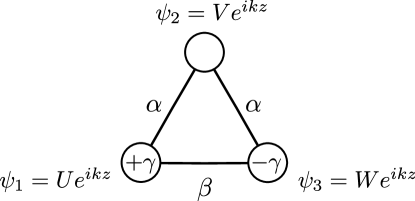
Figure 1: A schematic illustration of three coupled equations described by Eqs. (I). A conservative waveguide carrying the field $\psi_{2}$ is coupled to a ${\cal PT}$-symmetric (for $\gamma>0$) dimer of a gain and lossy waveguides carrying the fields $\psi_{1}$ and $\psi_{3}$, respectively. $\alpha$ and $\beta$ are the respective coupling coefficients.

II Solitons in the conservative model

Before considering solitons in the ${\cal PT}$-symmetric model, it is of fundamental importance to understand the properties of the underlying conservative model. To this end, in this section we address the case $\gamma=0$ in (I). We start looking for radial stationary soliton solutions of the form:

$$\psi_{\{1,2,3\}}=\{U(r),V(r),W(r)\}e^{ikz},$$

where $U$, $V$ and $W$ are real functions of the radius $r=\sqrt{x^{2}+y^{2}}$ in the $(x,y)$ plane and $k$ is the propagation constant.

The stationary wavefunctions $U$, $V$ and $W$ solve the system

$$-kU+\frac{d^{2}U}{dr^{2}}+\frac{1}{r}\frac{dU}{dr}+F(|U|)U+\alpha V+\beta W = 0,\ \ \$$

$$-kV+\frac{d^{2}V}{dr^{2}}+\frac{1}{r}\frac{dV}{dr}+F(|V|)V+\alpha U+\alpha W = 0,\ \ \$$ (6)

$$-kW+\frac{d^{2}W}{dr^{2}}+\frac{1}{r}\frac{dW}{dr}+F(|W|)W+\alpha V+\beta U = 0.\ \ \$$

The requirement of the regularity of the fields $\psi_{1,2,3}(x,y,z)$ at the origin $x=y=0$ implies the following boundary condition at $r=0$: $\left.dU/dr\right|_{r=0}=\left.dV/dr\right|_{r=0}=\left.dW/dr\right|_{r=0}=0$. On the other hand, looking for spatially localized solutions satisfying $\psi_{1,2,3}(x,y,z)\to 0$ as $x^{2}+y^{2}\to\infty$, we require functions $U$, $V$, and $W$ to vanish at the infinity: ${U,V,W}\to 0$ as $r\to\infty$.

II.1 Solutions in the limit $\alpha=0$

In order to classify possible solutions of the system (II), it is convenient to start with the limit $\alpha\to 0$ in which system of three equations (II) splits into two simpler subsystems whose properties are fairly well understood. The first subsystem is a single CQ-NLSE equation for the wavefunction $V$. It is known that, besides of the trivial zero solution, this equation admits a well-studied solitonic solution Quiroga ; Michinel ; Paredes . The second subsystem consists of two coupled equations for functions $U$ and $W$. Besides of the zero solution, this system admits a branch of symmetric solutions, for which $U=W$ and an asymmetric branch with $U\neq W$ Malomedcouplings . Thus combining the solutions from the two subsystems, we can predict the existence of five different nontrivial branches of solutions for the whole system of three equations (II) which can be continued to small but nonzero $\alpha$. The solutions of different types can be listed in the following order:

• Solution $1$ is a combination of the symmetric solution for the $U$-$W$ subsystem with the zero solution from the $V$-equation;

• Solution $2$ is a combination of the asymmetric solution for the $U$-$W$ subsystem with the zero solution from the $V$-equation;

• Solution $3$ bears trivial zero solution in the $U$-$W$ subsystem, but the nontrivial solitonic one for the $V$-equation;

• Solution $4$ is the combination of the symmetric solution for the $U$-$V$ coupler with the nonzero solution for the $V$-equation.

• Solution $5$ is the combination of the asymmetric solution for the $U$-$V$ coupler with the nonzero solution for the $V$-equation.

These considerations are systematized in the Table 1 (see the column $\alpha=0$). Examples of the listed solutions are displayed in the left column of Fig. 2 and Fig. 3.

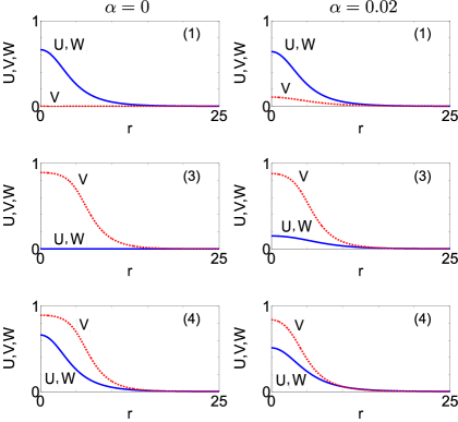
Figure 2: (Color online). Examples of symmetric solutions ($U=W$) of the conservative system found for $k=0.15$ and $\beta=0.07$. The left column presents the profiles for $\alpha=0$ and the right column for $\alpha=0.02$. The solid blue line shows $U$ and $W$, and the dashed red one shows $V$. The number on the right upper side indicates the label of the corresponding symmetric branch.

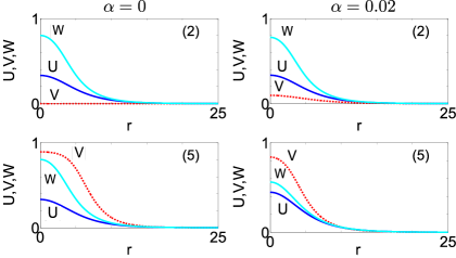
Figure 3: (Color online). Profiles of asymmetric solutions of the conservative coupled waveguides. The values of the parameters are the same that in Fig. 2 and each column shows again the solutions for $\alpha=0$ and $\alpha=0.02$ respectively. The blue and cyan continuous lines correspond to $U$ and $W$, and the dashed red line to $V$. The number on the right upper side indicates the label of the corresponding asymmetric branch.

Branch No.	symmetry	$\alpha=0$	arbitrary $\alpha$	stability (for $\alpha>0$)
1	sym	$U=W\neq 0$, $V=0$	does not exist for $\alpha>\alpha_{cr}$, see Eq. (11)	unstable for small $\alpha$,
				but becomes stable after bifurcation with branch 2
2	asym	$U\neq W$, $V=0$	does not exist after the pitchfork bifurcation	stable
3	sym	$U=W=0$, $V\neq 0$	merges with branch 4	stable
4	sym	$U=W\neq 0$, $V\neq 0$	merges with branch 3	unstable
5	asym	$U\neq W$, $V\neq 0$	does not exist after the pitchfork bifurcation	unstable

Table 1: Summary of the main features of the five branches of solutions of the conservative system.

II.2 Continuation over the coupling parameter $\alpha$

We use the five solutions identified above in the limit $\alpha\to 0$ as the initial guesses for the numerical continuation over the coupling parameter $\alpha$. Our numerical results are obtained rewriting the system of equations (II) in a finite differences scheme. We introduce a discrete spatial grid in the finite interval $r\in[0,R]$, where $R\gg 1$ is sufficiently large. The zero boundary condition at $r\to\infty$ is approximated by the requirement $U(R)=V(R)=W(R)=0$. Given the initial ansatz, solutions are found by a standard Newton-Raphson method (see Ref. diff for details about the finite differences and Newton-Raphson methods). Each of the five solutions can be continued to nonzero $\alpha$ originating in this way a continuous branch of solutions. The transformation of the soliton shapes under growing $\alpha$ can be traced by comparing the spatial profiles of the solitons in Fig. 2 (symmetric solutions) and Fig. 3 (asymmetric solutions). One observes that for $\alpha>0$ branches $1$, $3$ and $4$ remain symmetric: i.e., for these branches $U=W$ in the whole range of their existence. Branches $2$ and $5$ are asymmetric, i.e., they do not bear any particular symmetry among the three wavefunctions. Switching on $\alpha$ leads to growth of the second component in the solutions from the branches $1$ and $2$ (recall that for the corresponding solutions in the limit $\alpha=0$ the second component vanishes, $V=0$). In a similar way, branch $3$ has $U=W=0$ for $\alpha=0$, but nonzero $U$ and $W$ ($U=W$) for nonzero $\alpha$.

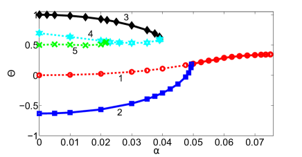
Figure 4: (Color online). Branches of the solutions on the plane $(\Theta,\alpha)$ for $k=0.15$ and $\beta=0.07$. The red circles correspond to solutions of type $1$, blue squares to type $2$, black diamonds to type $3$, cyan hexagons to type $4$, and green crosses to type $5$. Dashed lines indicate unstable solutions, and solid lines show stable solutions.

The complete bifurcation diagram obtained numerically after the continuation over the parameter $\alpha$ is visualized in Fig. 4 in the plane $(\Theta,\alpha)$, where the quantity $\Theta$ is defined as

$$\Theta=\frac{E_{U}+E_{V}-E_{W}}{E},$$ (7)

where

$$E_{\{U,V,W\}}=2\pi\int_{0}^{\infty}|\{U,V,W\}|^{2}rdr,$$ (8)

are the energies in the corresponding waveguides and

$$E=E_{U}+E_{V}+E_{W}.$$ (9)

is the total energy in the system.

The choice of the parameter to characterize bifurcations is not unique. We found $\Theta$ convenient as for the symmetric dimer solutions (the field propagates only in the waveguides $U$ and $V$ at $\alpha=0$) $\Theta=0$ and for the asymmetric solutions it describes the energy imbalance in the dimer. On the other hand, at $\alpha=0$, when energy propagates only along the conservative waveguide, we have $\Theta=1$. Alternatively, a similar diagram plotted in the plane $E$ vs $\alpha$ might be thought to be more conventional, but it does not allow to resolve easily the important bifurcation features, since many of the solutions have very close (or virtually equal) energies $E$. Notice also that since the conservative system is invariant under the interchange of $U$ and $W$, any asymmetric solution from branches $2$ and $5$ exists in two “copies”: $(U,V,W)$ and $(W,V,U)$ which obviously have different $\Theta$-characteristics. However, since these two copies can be easily obtained one from another, we show only one $\Theta$-dependence for each asymmetric branch, which makes the bifurcation diagram somewhat simpler and easier to read.

The most visible feature observable in Fig. 4 is that at certain $\alpha$ the asymmetric branch $2$ (blue squares) merges with the symmetric branch $1$ (red circles). This scenario can be considered as the symmetry breaking through a pitchfork bifurcation. After the bifurcation, symmetric branch $1$ can be continued until a certain critical value of $\alpha$ at which the solutions lose the exponential localization. The critical value of $\alpha$ can be computed if one looks at the asymptotic behavior of the soliton tails. Assuming that the behavior of the solutions for large $r$ is given by the following law: $U,V,W\propto\frac{1}{\sqrt{r}}e^{-\Lambda r}$, one can compute

$$\Lambda^{2}=k-\frac{1}{2}\sqrt{\beta^{2}+8\alpha^{2}}-\frac{1}{2}\beta.$$ (10)

The requirement $\Lambda^{2}>0$ implies that $\alpha<\alpha_{cr}$, where the critical coupling equals

$$\alpha_{cr}=\frac{1}{\sqrt{2}}\sqrt{k(k-\beta)}.$$ (11)

It also follows from (11) that the propagation constant $k$ must be larger than $\beta$: $k>\beta$. For the parameters in Fig. 4, we have $\alpha_{cr}\approx 0.077$.

The symmetry-breaking scenario in Fig. 4 can also be observed when the asymmetric branch $5$ (green crosses) meets the symmetric branch $4$ (cyan hexagons). After this, the asymmetric branch disappears, and only the symmetric branch $4$ exists. For larger $\alpha$, the symmetric branch $4$ merges with the symmetric branch  $3$ (black diamonds) featuring a saddle-node bifurcation.

II.3 Stability analysis

We have also examined the linear stability of the found solutions. Following the standard procedure, we considered perturbed solutions

$$\psi_{1}=e^{ikz}\big{[}U(r)+U_{+}(r)e^{in\theta}e^{\sigma z}+U_{-}^{*}(r)e^{-in\theta}e^{\sigma^{*}z}\big{]},\ \$$

$$\psi_{2}=e^{ikz}\big{[}V(r)+V_{+}(r)e^{in\theta}e^{\sigma z}+V_{-}^{*}(r)e^{-in\theta}e^{\sigma^{*}z}\big{]},\quad$$ (12)

$$\psi_{3}=e^{ikz}\big{[}W(r)+W_{+}(r)e^{in\theta}e^{\sigma z}+W_{-}^{*}(r)e^{-in\theta}e^{\sigma^{*}z}\big{]},$$

where $U_{\pm}(r)$, $V_{\pm}(r)$ and $W_{\pm}(r)$ describe radial behavior of small perturbations, $n=0,1,\ldots$ is the azimuthal index of the perturbation, $\theta$ is the polar angle, and $\sigma$ is the eigenvalue whose real part characterizes the instability growth rate. We derived the linear stability eigenvalue problem (see Appendix A), and computed the instability increment $\max(\textrm{Re}(\sigma))$. We have checked the lowest azimuthal indices with $n=0,1,2,3$, and found that the unstable eigenvalues (if any) are always generated by the perturbation with $n=0$, while the perturbations with $n\geq 1$ do not cause any instability (a similar observation for the system of two equations has been reported in Malomedcouplings ).

Linear stability results (also indicated in Fig. 4) show that in the limit $\alpha=0$ and for small $\alpha$ asymmetric branch $2$ and symmetric branch $3$ are stable. The symmetric branch $1$ is unstable for small $\alpha$ due to a pair of purely real unstable eigenvalues in the stability spectrum [Fig. 5(a)], but becomes stable [Fig. 5(b)] after the symmetry breaking bifurcation which connects branches $1$ and $2$ (thus the symmetry breaking pitchfork bifurcation connecting branches $1$ and  $2$ can be characterized as supercritical with respect to the parameter $1/\alpha$). Symmetric branch $4$ is unstable in the whole range of its existence. The instability is caused by two pairs of real unstable eigenvalues before the symmetry-breaking bifurcation with asymmetric branch $5$ [Fig. 5(c)]; after the bifurcation, branch $4$ is unstable due to only one pair of real eigenvalues [Fig. 5(d)]. Branch $5$ has a stable solution with $\alpha=0$ but becomes unstable (with one pair of real eigenvalues) for any nonzero $\alpha$.

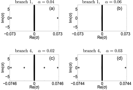
Figure 5: (a,b) The linear stability spectrum for the solution from the symmetric branch $1$ with $k=0.15$, $\beta=0.07$ and two different $\alpha$. (c,d) The linear stability spectrum for the solutions from the symmetric branch $4$ with $k=0.15$, $\beta=0.07$ and two different $\alpha$.

The stability of the solutions was also checked by means of the direct propagation of the stationary solitons. The input stationary profiles were slightly perturbed as

$$\psi_{1}(x,y,0) = U(r)\,(1-\epsilon),\quad$$

$$\psi_{2}(x,y,0) = V(r)\,(1+0.2\epsilon),$$ (13)

$$\psi_{3}(x,y,0) = W(r)\,(1+0.8\epsilon),$$

where for numerical simulations we set $\epsilon=0.03$. The propagation of the perturbed solutions was simulated by means of a split-step pseudo-spectral method, specifically the so-called Beam Propagation Method (BPM) bpm1 in a lattice of 512$\times$512 points. This explicit method is conditionally stable, so that a sufficiently small step $\Delta z$ must be considered bpm2 . Even though the scheme is of the first order in $\Delta z$, the evolution associated to the non-derivative terms was computed with a fourth order Runge-Kutta method. The perturbed solutions were propagated to a long distance ($z\gtrsim 600$) to observe their evolution.

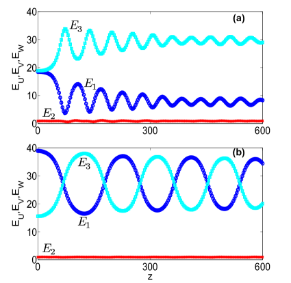
Figure 6: (Color online). (a) Plot of the energies in each waveguide $E_{1,2,3}=\int_{\mathbb{R}^{2}}|\psi_{1,2,3}|^{2}dxdy$ vs. propagation distance $z$ for the unstable symmetric solution from branch $1$ with $k=0.15$, $\beta=0.07$ and $\alpha=0.02$. (b) Plot of the energies $E_{1,2,3}$ vs. propagation distance $z$ for the unstable asymmetric solution from branch $2$ with $k=0.174$, $\beta=0.07$ and $\alpha=0.02$. While the $z$-axis of panel (b) is limited to $z=600$, we have checked that the shown regular oscillations of the energies persist until $z=3500$. For larger propagation distances (not shown in the figure), the solution loses spatial localization.

The results obtained from the simulation of the beam propagations agree with the above conclusions on the linear stability analysis.
For stable solutions, amplitude of the perturbation does not grow. For unstable solutions, the growing perturbation destroys the solutions which eventually become non-localized and lose completely their original shape. However, unstable solutions from branches $1$, $2$ and $3$ can preserve localization for significantly long propagation distance. During this long transient period, the instability manifests itself in almost periodic power oscillations whose amplitude decreases slowly. An example of such a behavior for an initially symmetric unstable solution from branch $1$ is illustrated in Fig. 6(a) and Fig. 7. As shown in Fig. 7, the initially symmetric solution develops strong asymmetry. Fig. 6(b) and Fig. 8 illustrate the development of almost periodic oscillations for an unstable asymmetric mode from branch 2.

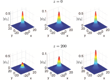
Figure 7: (Color online). Snapshots of the unstable initially symmetric solution whose propagation is shown in Fig. 6(a). The plots of the first file show the initial solution, and the plots of the second one correspond to $z=200$.

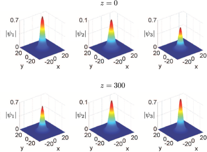
Figure 8: (Color online). Snapshots of the unstable solution whose propagation is shown in Fig. 6(b). The plots of first file show the initial solution, and the plots of the second one correspond to $z=300$.

II.4 Families of solutions: continuation over the propagation constant $k$

As the next step, we constructed families of the solutions $\Theta(k)$ (continuing solutions of the stationary problem over the propagation constant $k$ with all other parameters fixed). The obtained families are visualized in Fig. 9 on the plane $(\Theta,k)$. Similarly to what has been observed in Malomedcouplings for a coupler, we obtain that the possible values of the propagation constant belong to the range from $k_{min}=\beta$ up to $k_{max}=\beta+3/16$, where $k_{0}=3/16$ is the maximal value in the single 2D CQ-NLSE model Prytula in view of the divergence of the total energy $E$.

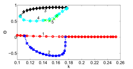
Figure 9: (Color online). Families of solutions on the plane $(\Theta,k)$ for $\beta=0.07$ and $\alpha=0.02$. In both panels, the red circles correspond to solutions of type $1$, blue squares to type $2$, black diamonds to type $3$, cyan hexagons to type $4$, and green crosses to type $5$. Dashed lines indicate unstable solutions, and solid lines show stable solutions.

The bifurcation diagram in Fig. 9 also features the symmetry breaking where the asymmetric family $2$ (blue squares) branches off from the symmetric family $1$ via a pitchfork bifurcation. The diagram also shows the exchange of stability which takes place after the bifurcation.

III ${\cal PT}$-symmetric solitons

III.1 ${\cal PT}$ symmetry breaking in the linear model

Before proceeding to the solitonic solutions in the nonlinear ${\cal PT}$-symmetric model (I) with $\gamma>0$, we recall the features of ${\cal PT}$-symmetry breaking in the underlying linear model. Omitting for the time being the CQ nonlinear part, we make the Fourier transform of the resulting linear model. Introducing $\hat{\psi}_{j}=\int_{-\infty}^{\infty}\int_{-\infty}^{\infty}e^{ik_{x}x+ik_{y}y}\psi_{j}(x,y,z)dxdy$, and the column vector $\hat{\psi}=(\hat{\psi}_{1},\hat{\psi}_{2},\hat{\psi}_{3})^{T}$, where $T$ stands for the transpose, we obtain

$$i\frac{\partial\hat{\psi}}{\partial z}=(k_{x}^{2}+k_{y}^{2})\hat{\psi}-H\hat{\psi}$$ (14)

where

$$\quad H=\begin{pmatrix}-i\gamma&\alpha&\beta\\ \alpha&0&\alpha\\ \beta&\alpha&i\gamma\end{pmatrix}.$$ (15)

The linear waves of the system are stable (and hence ${\cal PT}$ symmetry is unbroken) if all the eigenvalues of the matrix $H$ are real. The spectrum of (15) can be easily found Leykam . In particular the condition of the unbroken ${\cal PT}$ symmetry reads

$$\gamma^{2}\leq\gamma_{\cal PT}^{2}=2\alpha^{2}+\beta^{2}-3\sqrt[3]{\alpha^{4}\beta^{2}}.$$ (16)

Condition (16) implies that for any $\alpha$ and $\beta$ there exists a ${\cal PT}$-symmetry breaking threshold $\gamma_{\cal PT}$ such that ${\cal PT}$ symmetry is unbroken if $0\leq\gamma\leq\gamma_{\cal PT}$, but becomes broken otherwise. For the case of the homogeneous coupling, i.e., for $\alpha=\beta$ one has $\gamma_{\cal PT}=0$ LiKev , that is ${\cal PT}$ symmetry is broken for any nonzero gain-and-loss parameter $\gamma>0$.

III.2 Solitons

The system (I) admits stationary ${\cal PT}$-symmetric solitons in the form (II) where for $\gamma>0$ we assume that $U(r)=W^{*}(r)$ is, generically speaking, complex-valued function, and $V(r)$ is a real-valued function. Substituting (II) in (I) and separating the wavefunction $U$ into real and imaginary parts, $U(r)=U_{\textrm{R}}(r)+iU_{\textrm{I}}(r)$, we arrive at the following system

$$\frac{d^{2}U_{\textrm{R}}}{dr^{2}}+\frac{1}{r}\frac{dU_{\textrm{R}}}{dr}+[U_{\textrm{R}}^{2}+U_{\textrm{I}}^{2}-(U_{\textrm{R}}^{2}+U_{\textrm{I}}^{2})^{2}]U_{\textrm{R}}-kU_{\textrm{R}}$$

$$+\alpha V+\beta U_{\textrm{R}}+\gamma U_{\textrm{I}}=0,$$

$$\frac{d^{2}V}{dr^{2}}+\frac{1}{r}\frac{dV}{dr}+(V^{2}-V^{4})V+2\alpha U_{\textrm{R}}-kV=0,\ \$$ (17)

$$\frac{d^{2}U_{\textrm{I}}}{dr^{2}}+\frac{1}{r}\frac{dU_{\textrm{I}}}{dr}+[U_{\textrm{R}}^{2}+U_{\textrm{I}}^{2}-(U_{\textrm{R}}^{2}+U_{\textrm{I}}^{2})^{2}]U_{\textrm{I}}-kU_{\textrm{I}}\quad$$

$$-\beta U_{\textrm{I}}-\gamma U_{\textrm{R}}=0.$$

In order to obtain ${\cal PT}$-symmetric solitons with $\gamma>0$, we use the numerical continuation from the conservative limit $\gamma=0$. As follows from the requirement $U(r)=W^{*}(r)$, we can calculate ${\cal PT}$-symmetric solitons starting only from the symmetric conservative solutions, i.e., from the solutions of branches $1$, $3$ and $4$. We have also checked the stability of all ${\cal PT}$-symmetric solutions following the previous linear stability analysis with the incorporation in the system of equations (A) the terms responsible for gain and loss.

As discussed above, all conservative solutions from branch $4$ are unstable. We have observed that ${\cal PT}$-symmetric solutions obtained from this branch by considering $\gamma>0$ remain unstable. Therefore, in what follows we focus on branches $1$ and $3$ which can generate stable ${\cal PT}$-symmetric solitons. Figure 10 and Fig. 11 display examples of numerically found ${\cal PT}$-symmetric solutions obtained by means of the continuation from branches $1$ and $3$. Notice a well-pronounced difference between the two types of solitons: for the solitons in Fig. 10, the amplitude of the cores with gain and losses is larger than the amplitude of the neutral core, i.e., $|U|=|W|>|V|$; while for the solitons in Fig. 11 we have $|V|>|U|=|W|$. In Fig. 10, the increase of $\gamma$ leads to the progressive increase of $|U|=|W|$, whereas in Fig. 11 the opposite takes place: the amplitudes $|U|=|W|$ decrease as the gain-and-loss parameter $\gamma$ increases.

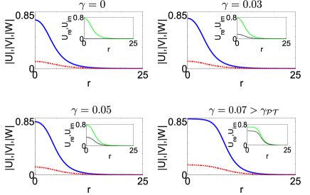
Figure 10: (Color online) Radial profiles of 2D ${\cal PT}$-symmetric solitons for the branch $1$ with $k=0.18$, $\beta=0.07$, $\alpha=0.02$ and different $\gamma$. For the chosen parameters, the ${\cal PT}$-symmetry breaking threshold equals to $\gamma_{{\cal PT}}\approx 0.054$. The solid blue line shows $|U|=|W|$, and the dashed red line shows $|V|$. In the insets, the real (solid green line) and imaginary (dashed black line) parts of $U$ are displayed.

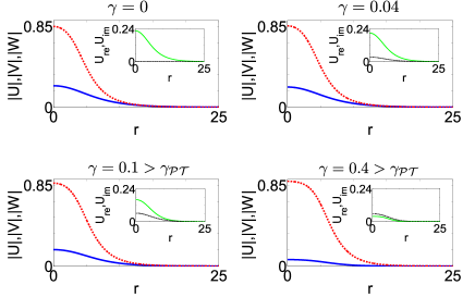
Figure 11: (Color online). Radial profiles of 2D PT-symmetric solitons for the branch $3$ with $k=0.15$, $\beta=0.07$, $\alpha=0.03$ and different values of $\gamma$. For the chosen parameters, the ${\cal PT}$-symmetry breaking threshold equals to $\gamma_{{\cal PT}}\approx 0.044$. The solid blue line shows $|U|=|W|$, and the dashed red line shows $|V|$. The insets show the profiles for the real (solid green line) and imaginary (dashed black line) parts of $U$.

Our numerical results show that stable conservative solitons (with $\gamma=0$) give birth to ${\cal PT}$-symmetric solitons (with $\gamma>0$) which remain stable, at least for sufficiently small $\gamma$. Moreover, our results allow to conjecture that the ${\cal PT}$-symmetric solitons continued from a stable conservative soliton remain stable for any $\gamma$ below the ${\cal PT}$-symmetry breaking threshold (we however notice that an accurate analytical treatment is required in order to substantiate this conjecture; in the vicinity of the ${\cal PT}$-symmetry breaking, i.e., for $0<\gamma_{{\cal PT}}-\gamma\ll 1$ hypothetical instability can be present, but its increment is small (of order $10^{-3}$ or less), and the associated eigenfunction is poorly localized, which requires a nonpractically large spatial window in order to perform an accurate computation). Stable solutions propagate for indefinitely long distance without the growth of the initially introduced perturbation. Figures 12 and 13 show two representative examples, where the shape of a slightly perturbed initial beam is practically indistinguishable from the beam obtained after the long-distance propagation.

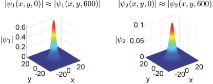
Figure 12: (Color online). Long-distance evolution of a stable 2D ${\cal PT}$-symmetric soliton from the branch $1$. The values of the parameters are the same as in Fig. 10 except for $\gamma=0.025$. The slightly perturbed initial beam propagates undistorted at least until $z=600$. The profile of $|\psi_{3}|$ is almost identical to $|\psi_{1}|$ and therefore is not shown.

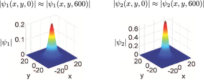
Figure 13: (Color online). Long-distance evolution of a stable 2D ${\cal PT}$-symmetric soliton from the branch $3$. The values of the parameters are the same as in Fig. 11 except for $\gamma=0.02$. The slightly perturbed initial beam propagates practically undistorted at least until $z=600$. The profile of $|\psi_{3}|$ is almost identical to $|\psi_{1}|$ and therefore is not shown.

The families of ${\cal PT}$-symmetric solitons can be numerically continued to arbitrarily large values of the gain-and-loss parameter $\gamma$ and, in particular, to the domain of the broken ${\cal PT}$ symmetry, i.e., to $\gamma>\gamma_{\cal PT}$, as this is typically occur in the stationary oligomer models Leykam ; LiKev ; trimer . However, all solitons with $\gamma>\gamma_{{\cal PT}}$ are unstable. Examples of such unstable solitons are shown in the two panels of Fig. 10 and Fig. 11 labeled as $\gamma>\gamma_{\cal PT}$ . Finally, we point out a difference between our system and the ${\cal PT}$-symmetric system of two equations Malomedgainloss : in the latter one no ${\cal PT}$ symmetric solitons (either stable or unstable) exists for $\gamma>\gamma_{\cal PT}$.

IV A note on interaction between solitons

In this section, we present a brief study on the interactions and collisions of the solitons described by (I). First, we analyzed interaction of asymmetric solitons in the conservative system. Initially quiescent solitons had a relative phase $\Delta\phi$ between them and were separated by a relatively small distance $\Delta x$. The respective initial distributions were prepared as follows:

$$\{U,V,W\}_{in}(x,y)=\{U,V,W\}_{st}(x-\Delta x,y)$$

$$+\{U,V,W\}_{st}(x+\Delta x,y)e^{i\Delta\phi}.$$ (18)

We have observed that in-phase solitons, $\Delta\phi=0$, attract each other and undergo inelastic collision after which they merge in a single pulse, as shown in Fig. 14. Out-of-phase solitons, $\Delta\phi=\pi$, repel each other, similarly to what happens in the system of two equations Malomedcouplings .

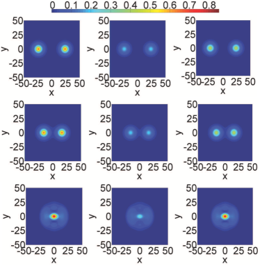
Figure 14: (Color online). Example of interaction between asymmetric solitons of the branch $2$ with $k=0.16$, $\beta=0.08$ and $\alpha=0.04$. The initial distance between them is $\Delta x=46$ and the relative phase $\Delta\phi=0$. The first, the second and the third columns visualize behavior of $\psi_{1}$, $\psi_{2}$ and $\psi_{3}$, respectively. The first, the second and the third rows correspond to $z=0$, $z=2300$ and $z=2558$, respectively.

We have also considered two ${\cal PT}$-symmetric solitons which were launched towards each other with an initial velocity from a certain distance. After the collision, the solitons combine one more time in a single pulse.

However, initially out-of-phase solitons, i.e., having initial relative phase $\Delta\phi=\pi$, do not recombine, but move outwards after the collision (see Fig. 15), and the distance between them grows indefinitely. The repulsion between the out-of-phase solitons is additionally illustrated in Fig. 16, which shows how the solitons do not cross at $x=0$.

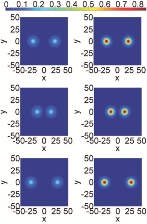
Figure 15: (Color online). Collision between ${\cal PT}$-symmetric solitons of the branch $3$ with $k=0.15$, $\beta=0.07$, $\alpha=0.03$ and $\gamma=0.02$. The initial distance between them is $\Delta x=46$, the relative phase $\Delta\phi=\pi$ and the velocity $v=0.02$. The first column shows $|\psi_{1}|=|\psi_{3}|$, and the second column visualizes the amplitude of the second component $\psi_{2}$. The first, the second and the third rows correspond to $z=0$, $z=264$ and $z=816$, respectively.

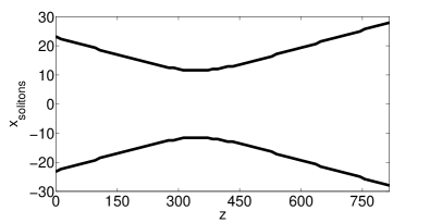
Figure 16: (Color online). Estimated positions in $x$ of the ${\cal PT}$-symmetric solitons of Fig. 15 vs. the propagation distance $z$. The continuous black lines indicate the positions of the solitons’ peaks. It can be appreciated how the repulsion prevents the cross of solitons at $x=0$.

V Conclusions

We have studied a model of a triple-core wave guide described by a system of three coupled two-dimensional nonlinear Schrödinger equations with the cubic (focusing) – quintic (defocusing) nonlinearity. In the first part of the work, we have considered the conservative case and classified possible families of bright solitons. The most interesting effect found is the symmetry-breaking bifurcation occurs at varying strength of the coupling or at growing propagation constant. The stability of the found solitons has been addressed in details.

In the second part of the work, we have extended the analysis onto the ${\cal PT}$-symmetric system, where one of the waveguides was lossy and another one active, with gain and losses balancing each other. We have demonstrated that such three-waveguide structure supports solitons. Two branches of solitons can be stable, at least for sufficiently weak gain-and-losses. Unlike in the case of two coupled equations Driben ; Malomedgainloss , the branches of ${\cal PT}$-symmetric solitons can be continued into the domain of arbitrarily strong gain-and-losses parameter. However, in this last limit the ${\cal PT}$-symmetry is broken what means instability of the solitons. Finally, the interactions and collisions between the solitons were briefly investigated. We observed merge of two in-phase solitons into a stable one and repelling of two out-of-phase solitons.

Appendix A Linear stability eigenvalue problem

The substitution of (II.3) in (I) and the subsequent linearization with respect to $U_{\pm}$, $V_{\pm}$ and $W_{\pm}$ leads to the following eigenvalue problem (we additionally assume $\gamma=0$):

$$i\sigma U_{+}+LU_{+}+2|U|^{2}U_{+}\quad\quad\quad\quad$$

$$+U^{2}U_{-}-3|U|^{4}U_{+}-2U^{3}U^{*}U_{-}+\alpha V_{+}+\beta W_{+}=0;\quad\quad\quad\quad$$

$$-i\sigma U_{-}+LU_{-}+2|U|^{2}U_{-}\quad\quad\quad\quad$$

$$+U^{2*}U_{+}-3|U|^{4}U_{-}-2U^{3*}UU_{+}+\alpha V_{-}+\beta W_{-}=0;\quad\quad\quad\ \$$

$$i\sigma V_{+}LV_{+}+2|V|^{2}V_{+}\quad\quad\quad\quad\ \$$

$$+V^{2}V_{-}-3|V|^{4}V_{+}-2V^{3}V^{*}V_{-}+\alpha U_{+}+\alpha W_{+}=0;\quad\quad\quad\quad$$ (19)

$$-i\sigma V_{-}+LV_{-}+2|V|^{2}V_{-}\quad\quad\quad\quad\ \$$

$$+V^{2*}V_{+}-3|V|^{4}V_{-}-2V^{3*}VV_{+}+\alpha U_{-}+\alpha W_{-}=0;\quad\quad\quad\ \$$

$$i\sigma W_{+}+LW_{+}+2|W|^{2}W_{+}\quad\quad\$$

$$+W^{2}W_{-}-3|W|^{4}W_{+}-2W^{3}W^{*}W_{-}+\alpha V_{+}+\beta U_{+}=0;\quad\quad\$$

$$-i\sigma W_{-}+LW_{-}+2|W|^{2}W_{-}\quad\quad\$$

$$+W^{2*}W_{+}-3|W|^{4}W_{-}-2W^{3*}WW_{+}+\alpha V_{-}+\beta U_{-}=0.\quad\quad\$$

Here the linear operator $L$ is defined as

$$L=\frac{d^{2}}{dr^{2}}+\frac{1}{r}\frac{d}{dr}-\frac{n^{2}}{r^{2}}-k,$$ (20)

$\sigma$ is the eigenvalue which characterizes the instability rate, and $n=0,1,2,\ldots$ is the azimuthal index of the perturbation.

References

- (1) C. Sulem and P.-L. Sulem, The Nonlinear Schrödinger Equation: Self-Focusing and Wave Collapse, Springer, vol. 139 (1999).
- (2) R. K. Dodd, J. C. Eilbeck, J. D. Gibbon and H. C. Morris Solitons and Nonlinear Wave Equations (Academic Press, Inc 1982).
- (3) M. Quiroga-Teixeiro and H. Michinel, J. Opt. Soc. Am. B 14, 2004 (1997); R. Radhakrishnan, A. Kundu, and M. Lakshmanan, Phys. Rev. E 60, 3314 (1999); A. Desyatnikov, A. Maimistov, and B. Malomed, Phys. Rev. E 61, (2000); R. L. Pego and H. A. Warchall, J. Nonlin. Sci. 12, 347 (2002); D. Mihalache, D. Mazilu, L.-C. Crasovan, I. Towers, A. V. Buryak, B. A. Malomed, L. Torner, J. P. Torres and F. Lederer, Phys. Rev. Lett. 88, 073902 (2002); Z. Birnbaum, B. A. Malomed, Physica D 237, 3252 (2008).
- (4) H. Michinel, J. Campo-Táboas, R. García-Fernández, J. R. Salgueiro, and M. L. Quiroga-Teixeiro, Phys. Rev. E 65, 066604 (2002).
- (5) M. J. Paz-Alonso, D. Olivieri, H. Michinel, and J. R. Salgueiro, Phys. Rev. E 69, 056601 (2004); D. Novoa, H. Michinel, D. Tommasini, Phys. Rev. Lett. 103, 023903 (2009); A. Paredes, D. Feijoo, and H. Michinel, Phys. Rev. Lett. 112, 173901 (2014); D. Feijoo, I. Ordónez, A. Paredes and H. Michinel, Phys. Rev. E 90, 033204 (2014).
- (6) Z.Wu, Y. Zhang, C. Yuan, F.Wen, H. Zheng, Y. Zhang, and M. Xiao, Phys. Rev. A 88, 063828 (2013); Y. Zhang, Z. Wu, M. R. Belić, H. Zheng, Z. Wang, M. Xiao, and Y. Zhang, Laser Photonics Rev. 9, no.3, 331 (2015).
- (7) S. V. Manakov, Zh. Eksp. Teor. Fiz. 65, 505 (1973) [Sov. Phys. JETP 38, 248 (1974)]; M. V. Tratnik and J. E. Sipe, Phys. Rev. A 38, 2011 (1988); D. N. Christodoulides and R. I. Joseph, Opt. Lett. 13, 53 (1988); C. R. Menyuk, IEEE J. Quant. Electron. 25, 3674 (1989); S. Trillo, S. Wabnitz, E. M. Wright, and G. I. Stegeman, Opt. Commun. 70, 166 (1989); B. A. Malomed, Phys. Rev. A 43, 410 (1991); V. M. Eleonskii, V. G. Korolev, N. E. Kulagin, and L. P. Shil’nikov, Zh. Eksp. Teor. Fiz. 99, 1113 (1991) [Sov. Phys. JETP 72, 619 (1991).];
- (8) S. Trillo, S. Wabnitz, E. M. Wright, and G. I. Stegeman, Opt. Lett. 13, 871 (1988); V. V. Afanas’ev, Yu. S. Kivshar, V. V. Konotop, and V. N. Serkin, Opt. Lett. 14, 805 (1989).
- (9) S. Trillo, S. Wabnitz, E. M. Wright, and G. I. Stegeman, Opt. Lett. 13, 672 (1988).
- (10) E. M. Wright, G. I. Stegeman, and S. Wabnitz, Phys. Rev. A 40, 4455 (1989); C. Paré, M. Florjańczyk, Phys. Rev. A 41, 6287 (1990); P. L. Chu, B. A. Malomed, G. D. Peng, JOSA B 10, 1379 (1993); N. Akhmediev and A. Ankiewicz, Phys. Rev. Lett. 70, 2395 (1993); J. M. Soto-Crespo and N. Akhmediev, Phys. Rev. E 48, 4710 (1993); N. Akhmediev and J. M. Soto-Crespo, Phys. Rev. E 49, 4519 (1994); B. A. Malomed, I. M. Skinner, P. L. Chu, G. D. Peng, Phys. Rev. E 53, 4084 (1996).
- (11) N. Dror and B. A. Malomed, Physica D 240, 526–541 (2011).
- (12) see e.g. Y. Kawaguchia, M. Ueda, Phys. Rep. 520, 253 (2012).
- (13) C. M. Bender and S. Boettcher, Phys. Rev. Lett. 80, 5243 (1998); C. M. Bender, Rep. Prog. Phys. 70, 947 (2007).
- (14) C. E. Rüter, K. G. Makris, R. El-Ganainy, D. N. Christodoulides, M. Segev, and D. Kip, Nature Physics 6, 192 (2010).
- (15) R. Driben and B. A. Malomed, Opt. Lett. 36, 4323 (2011); F. K. Abdullaev, V. V. Konotop, M. Ögren, and M. P. Sørensen, Opt. Lett. 36, 4566 (2011); N. V. Alexeeva, I. V. Barashenkov, A. A. Sukhorukov, and Y. S. Kivshar, Phys. Rev. A 85, 063837 (2012); Y. V. Bludov, R. Driben, V. V. Konotop, and B. A. Malomed, J. Opt. 15, 064010 (2013); Y. V. Bludov, C. Hang, G. Huang, and V. V. Konotop, Opt. Lett. 39, 3382 (2014).
- (16) G. Burlak and B. A. Malomed, Phys. Rev. E 88, 062904 (2013).
- (17) L. Jin and Z. Song, Phys. Rev. A 80 052107 (2009); Y. N. Joglekar, D. Scott, M. Babbey and A. Saxena, Phys. Rev. A 82, 030103 (2010); I. V. Barashenkov, L. Baker, and N. V. Alexeeva, Phys. Rev. A 87, 033819 (2013); D. E. Pelinovsky, D. A. Zezyulin, and V. V. Konotop, J. Phys. A: Math. Theor. 47, 085204 (2014).
- (18) D. Leykam, V. V. Konotop, and A. S. Desyatnikov, Opt. Lett. 38 (2013).
- (19) K. Li, and P. G. Kevrekidis, Phys. Rev. E 83, 066608 (2011).
- (20) K. Li, P. G. Kevrekidis, D. J. Frantzeskakis, C. E. Rüter and D. Kip, J. Phys. A: Math. Theor. 46, 375304 (2013); M. Duanmu, K. Li, R. L. Horne, P. G. Kevrekidis and N.Whitaker, Phil Trans R Soc A 371, 20120171 (2013).
- (21) H. M. Antia, Numerical Methods for Scientists and Engineers, Springer Science and Business Media (2002); R. J. LeVeque, Finite Difference Methods for Ordinary and Partial Differential Equations: steady state and time-dependent problems, Siam (2007).
- (22) G. P. Agrawal, Nonlinear Fiber Optics (Elsevier, New York, 4th ed.) (2006) ; T.-C. Poon and T. Kim, Engineering Optics with MATLAB (World Scientific, Singapore, 2006).
- (23) J. A. C.Weideman and B. M. Herbst, SIAM J. Numer. Anal. 23, 485 (1986) ; T. I. Lakoba, Numer. Methods Partial Differ. Equ. 28, 641 (2012).
- (24) I. Towers, A.V. Buryak, R. A. Sammut, B.A. Malomed, L.-C. Crasovan and D. Mihalache, Phys. Lett. A 288 (2001) 292-298; B.A. Malomed, G.D. Peng, P.L. Chu, I. Towers, A.V. Buryak, R.A. Sammut, Pramana 57 (2001) 1061-1078; V. Prytula, V. Vekslerchik, and V. M. Pérez-García, Phys. Rev. E 78, 027601 (2008).