Description of electromagnetic and favored $\alpha$-transitions in heavy odd-mass nuclei

Abstract

We describe electromagnetic and favored $\alpha$-transitions to rotational bands in odd-mass nuclei built upon a single particle state with angular momentum projection $\Omega\neq\frac{1}{2}$ in the region $88\leq Z\leq 98$. We use the particle coupled to an even-even core approach described by the Coherent State Model (CSM) and the coupled channels method to estimate partial $\alpha$-decay widths. We reproduce the energy levels of the rotational band where favored $\alpha$-transitions occur for 26 nuclei and predict $B\left(E2\right)$ values for electromagnetic transitions to the bandhead using a deformation parameter and a Hamiltonian strength parameter for each nucleus, together with an effective collective charge depending linearly on the deformation parameter. Where experimental data is available, the contribution of the single particle effective charge to the total $B\left(E2\right)$ value is calculated. The Hamiltonian describing the $\alpha$-nucleus interaction contains two terms, a spherically symmetric potential given by the double-folding of the M3Y nucleon-nucleon interaction plus a repulsive core simulating the Pauli principle and a quadrupole-quadrupole (QQ) interaction. The $\alpha$-decaying state is identified as a narrow outgoing resonance in this potential. The intensity of the transition to the first excited state is reproduced by the QQ coupling strength. It depends linearly both on the nuclear deformation and the square of the reduced width for the decay to the bandhead, respectively. Predicted intensities for transitions to higher excited states are in a reasonable agreement with experimental data. This formalism offers a unified description of energy levels, electromagnetic and favored $\alpha$-transitions for known heavy odd-mass $\alpha$-emitters.

I Introduction

A brief overview of the $\alpha$-emission process in even-even nuclei is helpful for the understanding of the more complex situation in odd-mass emitters.

In the case of transitions to excited states, the single-particle levels around the Fermi surface play the dominant role and the corresponding decay widths are very sensitive to the structure of the daughter nucleus Del10 ; Buc12 . An important problem is the study of the $\alpha$-daughter interaction. One of the most popular approaches is the double folding procedure Neu92 . This method has been used together with the coupled channels approach and a repulsive core simulating the Pauli principle in order to study the $\alpha$-decay fine structure in transitional and rotational even-even nuclei Del06 . For a thorough study of the structure and $\alpha$-emission spectrum in vibrational, transitional and rotational even-even nuclei, see Ref. Del15 .

Several calculations for the fine structure of the emission spectrum have already been made in the case of odd-mass $\alpha$-emitters. For example, in Ref. Ni12 a multichannel cluster model together with the coupled channels equation is used to calculate branching ratios to excited states for favored transitions in heavy emitters, in the region $93<Z<102$. In Ref. War15 , a microscopic method is employed with a Skyrme SLy4 effective interaction. Starting from the Hartree-Fock-Bogoliubov vacuum and quasiparticle excitations, the $\alpha$-particle formation amplitude is calculated for the $\alpha$-decay to various channels mostly in the $84<Z<88$ region. Several unfavored transitions are treated in this paper and predictions are made for the properties of the g.s.$\rightarrow$g.s. $\alpha$-trasition in odd-mass superheavy nuclei. The unfavored g.s.$\rightarrow$g.s. $\alpha$-decay in odd-mass nuclei in the region $64\leq Z\leq 112$ is also treated in Ref. Sei15 , with the purpose of investigating the effect of the difference in the spin and parity of the ground states on the $\alpha$-particle and daughter nucleus preformation probability. The calculations are done in the framework of the extended cluster model, with the Wentzel-Kramers-Brillouin penetrability and assault frequency, together with an interaction potential computed on the basis of the Skyrme SLy4 interaction.

In the current paper, we expand the method previously used in Ref. Del15 for the even-even case by allowing the coupling of an odd-particle to a core described by a coherent function. We study the energy levels and electromagnetic transition rates of this nucleus and then couple an $\alpha$-particle to it in order to describe the emission spectrum for the case of favored transitions. Our method is to employ an $\left(I,l\right)$ coupling procedure in the laboratory frame, between the angular momentum $I$ of the daughter nucleus and the orbital angular momentum $l$ of the $\alpha$-particle, similar to Nilsson’s original $\left(I,j\right)$ coupling method for the description of nuclear spectra in the intrinsic frame Nil , where $j$ is the angular momentum of the odd particle. We show that using a small basis having a single value for $l$ in each channel, we can use a QQ $\alpha$-daughter interaction to generate simultaneously resonant states of even or odd parity at the same reaction energy and QQ coupling strength. The partial decay widths obtained this way are in good agreement with the available experimental data.

II Theoretical Background

In this section we present the theoretical tools required for the calculation of energy levels and electromagnetic transition rates for odd-mass nuclei, as well as the coupled-channels method that is applied to the study of the fine structure of the $\alpha$-emission spectrum.

II.1 Nucleon coupled to a coherent state core

A description of the surface dynamics of a deformed even-even nucleus was proposed for the first time in Refs. Lip69 ; Lip76 by using a coherent state of quadrupole bosons. A generalization to all types of low-energy collective motion was proposed in Refs. Rad76a ; Rad76b and was extensively developed in Refs. Rad81 ; Rad82 as the coherent state model (CSM). A review paper on this topic is available in Ref. Rad12 , as well as in the textbook Rad14 . Here, we will present in a concise manner the main ideas of the model, and then extend them to the coupling of an additional nucleon to the even-even core. The final goal is to describe a rotational band built upon a given single-particle state of the odd nucleon.

We begin by assuming that the intrinsic state of an axially deformed even-even nucleus is given by a coherent superposition of quadrupole bosons $b^{\dagger}_{2\mu}$ with $\mu=0$

$$|\phi_{g}\rangle=e^{d\left(b^{{\dagger}}_{20}-b_{20}\right)}|0\rangle,$$ (1)

where $|0\rangle$ is the phonon vacuum and the quantity $d$ is called deformation parameter Rad81 .

The physical states that define the ground band are obtained by angular momentum projection

$$|\varphi_{JM}^{\left(g\right)}\rangle=\mathcal{N}_{J}^{\left(g\right)}P^{J}_{M0}|\phi_{g}\rangle.$$ (2)

$P_{M0}^{J}$ is the projection operator which has the integral representation

$$P^{J}_{MK}=\sqrt{\frac{2J+1}{8\pi^{2}}}\int{d\omega}\mathcal{D}^{J}_{MK}\left(\omega\right)R\left(\omega\right),$$ (3)

with $\omega$ the set of three Euler angles, $\mathcal{D}^{J}_{MK}\left(\omega\right)$ a Wigner function and $R\left(\omega\right)$ the rotation operator.

$\mathcal{N}_{J}^{\left(g\right)}$ is the norm of the projected state, given by the formula

$$\mathcal{N}_{J}^{\left(g\right)}=\left[\hat{J}^{2}\mathcal{I}_{J}^{\left(0\right)}\left(d\right)\right]^{-\frac{1}{2}}e^{\frac{d^{2}}{2}},$$ (4)

with $\hat{J}=\sqrt{2J+1}$ and $\mathcal{I}_{J}^{\left(0\right)}\left(d\right)$ given by

$$\mathcal{I}_{J}^{\left(0\right)}\left(d\right)=\int_{0}^{1}\mathcal{P}_{J}\left(x\right)e^{d^{2}\mathcal{P}_{2}\left(x\right)}dx,$$ (5)

in terms of the Legendre polynomial $\mathcal{P}_{J}$.

For an odd-mass nucleus, the state of total angular momentum $I$ and projection $M$ is given by projecting out the product between the coherent state (1) and the single particle state $\psi_{jm}$, where $j$ is a shorthand notation for all of the quantum numbers of the state, that is

$$\Phi_{IM}=P^{I}_{M0}\left[\psi_{j}\phi_{g}\right].$$ (6)

A straighforward calculation leads to the following result

$$\Phi_{IM}=\sum_{J}X_{I}^{Jj}\left[\varphi_{J}^{\left(g\right)}\otimes\psi_{jm}\right]_{IM},$$ (7)

with normalization coefficients $X_{I}^{Jj}$ given by

$$X_{I}^{Jj}=\frac{\left(\mathcal{N}_{J}^{\left(g\right)}\right)^{-1}\langle jJ;\Omega 0|I\Omega\rangle}{\sqrt{\sum\limits_{J^{\prime}}\left(\mathcal{N}_{J^{\prime}}^{\left(g\right)}\right)^{-2}\left(\langle jJ^{\prime}\Omega 0|I\Omega\rangle\right)^{2}}},$$ (8)

where the bra-ket product denotes a Clebsch-Gordan coefficient and $\Omega$ is the fixed z-projection of the single-particle angular momentum $j$. More details on this procedure can be consulted in Ref. Del93 .

The states built upon the bandhead $I=j=\Omega$ that follow the sequence $I=\Omega,\Omega+1,\Omega+2,\dots$ constitute a rotational band. In the Nilsson model, these states are labeled by the set $\Omega^{\pi}\left[Nn_{z}\Lambda\right]$, where $\pi$ is the parity, $N$ is the principal quantum number, $n_{z}$ the number of nodes of the radial wavefunction in the $z$ direction and $\Lambda$ the projection of the single-particle orbital angular momentum. The last three numbers act only as labels, as the good quantum numbers are only $\Omega$ and $\pi$.

The simplest Hamiltonian that can describe such a rotational structure consists of two terms Del93 :

$$H=A_{1}b^{\dagger}_{2}\cdot b_{2}-A_{2}r^{2}\left(b^{\dagger}_{2}+\tilde{b}_{2}\right)\cdot Y_{2}.$$ (9)

where by dot we denoted the scalar product. $A_{1}$ is a strength parameter required to fit experimental data and $A_{2}$ is the strength of the particle-core QQ interaction. For a given ladder operator $a_{l}$, we have

$$\tilde{a}_{l\mu}=\left(-\right)^{\mu}a_{l-\mu}.$$ (10)

For the description of the rotational band the only relevant parameter is $A_{1}$ due to the fact that the particle-core term is common. Instead of solving the eigenvalue problem by a full diagonalization procedure, a simpler approach, involving the analytical expression for the diagonal matrix elements of the Hamiltonian (9) in the basis of Eq. (7) suffices:

$$\langle IM|H|IM\rangle = A_{1}d^{2}f_{j\Omega I}-d\left(N+\frac{3}{2}\right)\times$$

$$\times \langle j2;\Omega 0|j\Omega\rangle\langle j2;\frac{1}{2}0|j\frac{1}{2}\rangle,$$

with $f_{j\Omega I}$ given by

$$f_{j\Omega I}=\frac{\sum\limits_{J}\langle Ij;\Omega-\Omega|J0\rangle^{2}\mathcal{I}_{J}^{\left(1\right)}\left(d\right)}{\sum\limits_{J}\langle Ij;\Omega-\Omega|J0\rangle^{2}\mathcal{I}_{J}^{\left(0\right)}\left(d\right)},$$ (12)

in terms of the function

$$\mathcal{I}_{J}^{\left(1\right)}\left(x\right)=\frac{d}{dx}\mathcal{I}_{J}^{\left(0\right)}\left(x\right).$$ (13)

The shape of such a spectrum is dependent both on the deformation parameter and on the value of $\Omega$, as can be seen in Fig. 1.

Figure 1: Normalized energy levels $E_{I}$ as function of deformation $d$, for different values of the single particle angular momentum projection $\Omega$.

While this approach is adequate for the purpose of this paper, if a greater precision in the description of the nuclear energy spectrum is required, then more terms can be added to the Hamiltonian (9), as shown in Ref. Del93 . Let us also mention that the development presented here and expanded upon in Ref. Del93 is appropriate for any rotational band built upon an angular momentum projection $\Omega\neq\frac{1}{2}$. The special case $\Omega=\frac{1}{2}$ requires a modification of the formalism and will be treated in a future paper.

II.2 Electromagnetic transitions

The $B\left(E2\right)$ values of electric quadrupole transitions follow from both collective and single particle contributions

$$B\left(E2;I_{2}\rightarrow I_{1}\right) = [\frac{1}{\hat{I}_{2}}\langle I_{1}||q_{0}^{c}Q^{c}_{2}||I_{2}\rangle+$$

$$+ \frac{1}{\hat{I}_{2}}\langle I_{1}||q_{0}^{sp}Q^{sp}_{2}||I_{2}\rangle]^{2},$$

where $q_{0}^{c}$ and $q_{0}^{sp}$ are effective charges.

The collective quadrupole transition operator has both harmonic and anharmonic contributions

$$Q^{c}_{2\mu}=b^{\dagger}_{2\mu}+\tilde{b}_{2\mu}+a_{q}\left[\left(b^{\dagger}_{2}\otimes b^{\dagger}_{2}\right)_{2\mu}+\left(b_{2}\otimes b_{2}\right)_{2\mu}\right],$$ (15)

with $a_{q}$ the anharmonic strength. Its reduced matrix elements on the states of the core are

$$\langle\varphi_{J_{1}}^{\left(g\right)}||q_{0}^{c}Q^{c}_{2}||\varphi_{J_{2}}^{\left(g\right)}\rangle = \frac{q_{eff}d}{\hat{J}_{2}\mathcal{N}_{J_{1}}^{\left(g\right)}\mathcal{N}_{J_{2}}^{\left(g\right)}}\langle J_{1}2;00|J_{2}0\rangle\times$$

$$\times \left[\hat{J}^{2}_{1}\left(\mathcal{N}_{J_{1}}^{\left(g\right)}\right)^{2}+\hat{J}_{2}^{2}\left(\mathcal{N}_{J_{2}}^{\left(g\right)}\right)^{2}\right],$$

with $q_{eff}$ given by a linear formula in $d$

$$q_{eff}=q_{0}^{c}\left(1-\sqrt{\frac{2}{7}}a_{q}d\right).$$ (17)

The single particle quadrupole transition operator has the occupation number representation

$$Q^{sp}_{2\mu}=\sum_{j_{1}j_{2}}\frac{1}{\hat{2}}\langle j_{1}||r^{2}Y_{2}||j_{2}\rangle\left(c^{\dagger}_{j_{1}}\tilde{c}_{j_{2}}\right)_{2\mu}.$$ (18)

Explicit expressions for the matrix elements of these operators over the states of the odd-mass nucleus follow from the above results and the use of standard angular momentum algebra. For our particular case of fixed $j$, the final formulas are

$$\langle I_{1}||q_{0}^{c}Q^{c}_{2}||I_{2}\rangle = \sum\limits_{J_{1}J_{2}}X_{I_{1}}^{J_{1}j}X_{I_{2}}^{J_{2}j}\hat{I_{1}}\hat{I_{2}}\left(-\right)^{j-I_{1}}\times$$

$$\times \mathcal{W}\left(I_{1}J_{1}I_{2}J_{2};j2\right)\langle\varphi_{J_{1}}^{\left(g\right)}||q_{0}^{c}Q^{c}_{2}||\varphi_{J_{2}}^{\left(g\right)}\rangle,$$

$$\langle I_{1}||q_{0}^{sp}Q^{sp}_{2}||I_{2}\rangle = \sum\limits_{J_{1}}X_{I_{1}}^{J_{1}j}X_{I_{2}}^{J_{1}j}\hat{I_{1}}\hat{I_{2}}\left(-\right)^{j+I_{2}}\times$$

$$\times \mathcal{W}\left(I_{1}jI_{2}j;J_{1}2\right)\langle j||q_{0}^{sp}r^{2}Y_{2}||j\rangle,$$

with $\mathcal{W}$ a Racah coefficient.

All reduced matrix elements are defined in the usual convention

$$\langle lm|T_{\lambda\mu}|l^{\prime}m^{\prime}\rangle=\frac{1}{\hat{l}}\langle l^{\prime}m^{\prime};\lambda\mu|lm\rangle\langle l||T_{\lambda}||l^{\prime}\rangle.$$ (21)

II.3 $\alpha$-emission in the coupled channels approach

The decay phenomenon of interest connects the ground state of the parent nucleus of angular momentum $I_{P}$ to an excited state of angular momentum $I$ of the daughter and an $\alpha$-particle of angular momentum $l$, in such a way that the total angular momentum $I_{P}$ is conserved:

$$P\left(I_{P}\right)\rightarrow D\left(I\right)+\alpha\left(l\right).$$ (22)

An important remark is that both the initial state of the parent and the final state of the daughter are built upon the same single particle orbital $j$. This is known as a favored $\alpha$-transition, due to the fact that it usually has a large branching ratio. The situation where the initial and final single particle orbitals are different is known as an unfavored $\alpha$-transition. For the favored case, the transition from the ground state to the bandhead built atop the $j$ orbital in the daughter nucleus generally has the highest decay width, and transitions on excited states of the band form the fine structure of the spectrum.

The total wavefunction of the $\alpha$-daughter system can be assumed to be separable in radial and angular parts and expanded in the angular momentum basis

$$\Psi\left(b^{\dagger}_{2},{\bf R}\right)=\sum_{Il}\frac{f_{Il}\left(R\right)}{R}\mathcal{Z}_{Il}\left(b^{\dagger}_{2},\omega\right),$$ (23)

where the angular components are given by the coupling to good angular momentum between a wave function for the odd-mass daughter nucleus and a spherical harmonic for the $\alpha$-particle

$$\mathcal{Z}_{Il}\left(b^{\dagger}_{2},\omega\right)=\left[\Phi_{IM}\left(b^{\dagger}_{2}\right)\otimes Y_{lm}\left(\omega\right)\right]_{I_{P}M_{P}}.$$ (24)

Here, ${\bf R}=\left(R,\omega\right)$ is the relative vector between the two fragments. Each pair of angular momentum values defines a decay channel

$$\left(I,l\right)=c.$$ (25)

The function $\Psi$ must satisfy the stationary Schrödinger equation

$$H\Psi\left(b^{\dagger}_{2},{\bf R}\right)=Q_{\alpha}\Psi\left(b^{\dagger}_{2},{\bf R}\right),$$ (26)

with $Q_{\alpha}$ the Q-value of the decay process. The Hamiltonian

$$H=-\frac{\hbar}{2\mu}{\bf\nabla}^{2}_{{\bf R}}+H_{D}\left(b^{\dagger}_{2}\right)+V\left(b^{\dagger}_{2},{\bf R}\right)$$ (27)

features a kinetic operator depending on the reduced mass $\mu$ of the system

$$\mu=m_{N}\frac{4A_{D}}{4+A_{D}},$$ (28)

a term describing the motion of the daughter $H_{D}\left(b^{\dagger}_{2}\right)$ and an $\alpha$-daughter interaction with monopole and quadrupole components

$$V\left(b^{\dagger}_{2},{\bf R}\right)=V_{0}\left(R\right)+V_{2}\left(b^{\dagger}_{2},{\bf R}\right).$$ (29)

A detailed study of this potential can be found in Ref. Del06 . There it is shown that the monopole component has a pocket-like shape

$$V_{0}\left(R\right) = v_{a}\bar{V}_{0}\left(R\right),R>R_{m}$$

$$= a\left(R-R_{min}\right)^{2}-v_{0},R<R_{m},$$

obtained through the matching of a harmonic oscillator to the nuclear plus Coulomb potential $\bar{V}_{0}$ obtained by the method of the double folding procedure of the M3Y particle-particle interaction with Reid soft core parametrisation (Refs. Ber77 ; Sat79 ; Car92 and the book Del10 for computational details).

The number $v_{a}$ acts as a quenching factor of the nuclear force. $v_{a}=1$ implies an $\alpha$-particle existing with certainty, and a value $v_{a}<1$ is required in order to simulate the formation of the $\alpha$-particle on the nuclear surface. Since branching ratios tend to have a weak dependence on this parameter Del06 , it can be adjusted in order to reproduce the total decay width $\Gamma$ Pel08 . Another possibility is to leave the interaction potential unquenched and to consider the spectroscopic factor

$$S=\frac{\Gamma_{expt}}{\Gamma_{theor}},$$ (31)

as a measure of the particle formation probability, as in Ref. Del15a .

The repulsive core on the second line of equation (II.3) simulates the Pauli principle, namely the fact that the $\alpha$-particle can exist only on the nuclear surface. Its parameters can be adjusted so that the first resonance in the potential corresponds to the experimental Q-value.

The matching radius $R_{m}$ and the point $R_{min}$ at which the oscillator potential attains the lowest value are found through the method of Ref. Del06 , which requires the equality between the external attraction and internal repulsion together with their derivatives. This makes the total interaction continuous and dependent on the repulsive strength $a$ and potential depth $v_{0}$. In our study, $a$ has a fixed value of $50\textrm{ MeV}$ for all nuclei and $v_{0}$ is fitted in each case through the experimental Q-value.

The second term of Eq. (29) is the QQ interaction

$$V_{2}\left(b^{\dagger}_{2},{\bf R}\right) = -C_{0}\left(R-R_{min}\right)\frac{dV_{0}\left(R\right)}{dR}\times$$

$$\times \sqrt{5}\left[Q^{c}_{2}\otimes Y_{2}\left(\omega\right)\right]_{0},$$

with $C_{0}$ serving as an $\alpha$-nucleus coupling strength.

The angular functions entering the expansion of Eq. (23) are orthonormal. Using this, one obtains in a standard way the system of coupled differential equations for radial components

$$\frac{d^{2}f_{I_{1}l_{1}}\left(R\right)}{d\rho_{I_{1}}^{2}}=\sum_{I_{2}l_{2}}A_{I_{1}l_{1};I_{2}l_{2}}\left(R\right)f_{I_{2}l_{2}}\left(R\right),$$ (33)

with the coupling matrix having the expression

$$A_{I_{1}l_{1};I_{2}l_{2}}\left(R\right) = \left[\frac{l_{1}\left(l_{1}+1\right)}{\rho_{I_{1}}^{2}}+\frac{V_{0}\left(R\right)}{Q_{\alpha}-E_{I_{1}}}-1\right]\delta_{I_{1}l_{1};I_{2}l_{2}}+$$ (34)

$$+ \frac{1}{Q_{\alpha}-E_{I_{1}}}\langle\mathcal{Z}_{I_{1}l_{1}}|V_{2}\left(b^{\dagger}_{2},{\bf R}\right)|\mathcal{Z}_{I_{2}l_{2}}\rangle,$$

in terms of the reduced radius

$$\rho_{I}=\kappa_{I}R,\textrm{ }\kappa_{I}=\sqrt{\frac{2\mu\left(Q_{\alpha}-E_{I}\right)}{\hbar^{2}}}.$$ (35)

Notice that $\kappa_{I}$ has the same value for all the channels of fixed $I$, so the supplementary $l$-index can be omitted both for the wave number and reduced radius.

The coupling term of the matrix is found by the same methods as in the previous sections to be

$$\langle\mathcal{Z}_{I_{1}l_{1}}|V_{2}\left(b^{\dagger}_{2},{\bf R}\right)|\mathcal{Z}_{I_{2}l_{2}}\rangle=$$ (36)

$$\sum\limits_{J_{1}J_{2}}X_{I_{1}}^{J_{1}j}X_{I_{2}}^{J_{2}j}\langle\varphi_{J_{1}}^{\left(g\right)}||Q_{2}^{c}||\varphi_{J_{2}}^{\left(g\right)}\rangle\langle l_{1}||Y_{2}||l_{2}\rangle\hat{I}_{P}^{2}\hat{I}_{1}\hat{I}_{2}\hat{j}$$

$$\times \left(-\right)^{I_{2}-I_{P}+l_{2}}\mathcal{W}\left(I_{1}l_{1}I_{2}l_{2};I_{P}2\right)\begin{Bmatrix}J_{1}&I_{1}&j\\ J_{2}&I_{2}&j\\ 2&2&0\end{Bmatrix}$$

where the curly brackets denote a 9j-symbol. Since the reduced matrix element between the states of the core is a linear function of the deformation Rad82 , one can express this linearity in terms of an effective $\alpha$-nucleus coupling strength having a different anharmonic parameter $a_{\alpha}$

$$C=C_{0}\left(1-\sqrt{\frac{2}{7}}a_{\alpha}d\right).$$ (37)

II.4 Resonant states

The measured $\alpha$-decay widths are by many orders of magnitude smaller than the Q-value. Thus, an $\alpha$-decaying state is almost a bound state, this being the main reason way the stationary approach is a very good approximation of the emission process. The state can be identified with a narrow resonant solution of the system of equations (33), containing only outgoing components. In order to solve this system of equations we first define the internal and external fundamental solutions which satisfy the boundary conditions

$${\cal R}_{Il,L}(R) \stackrel{{\scriptstyle R\rightarrow 0}}{{\longrightarrow}}\delta_{Il,L}\varepsilon_{Il}~{},$$

$${\cal H}_{Il,L}^{(+)}(R) \equiv{\cal G}_{Il,L}(R)+i{\cal F}_{Il,L}(R)\stackrel{{\scriptstyle R\rightarrow\infty}}{{\longrightarrow}}$$

$$\delta_{Il,L}H_{l}^{(+)}(\kappa_{I}R) \equiv\delta_{Il,L}\left[G_{l}(\kappa_{I}R)+iF_{l}(\kappa_{I}R)\right]~{},$$

where $\varepsilon_{Il}$ are arbitrary small numbers. Here, the channel indexes label the component and $L$ the solution, $G_{Il}(\kappa_{I}R)$ and $F_{Il}(\kappa_{I}R)$ are the standard irregular and regular spherical Coulomb functions, depending on the momentum $\kappa_{I}$ in the channel $c$, defined by Eq. (35).

Each component of the solution is built as a superposition of $N$ independent fundamental solutions. We impose the matching conditions at some radius $R_{1}$ inside the barrier and obtain

$$f_{Il}(R_{1}) = \sum_{L}{\cal R}_{Il,L}(R_{1})M_{Il,L}=\sum_{L}{\cal H}^{(+)}_{Il,L}(R_{1})N_{Il,L}$$ (39)

$$\frac{df_{Il}(R_{1})}{dR} = \sum_{L}\frac{d{\cal R}_{Il,L}(R_{1})}{dR}M_{Il,L}=\sum_{L}\frac{d{\cal H}^{(+)}_{Il,L}(R_{1})}{dR}N_{Il,L}~{},$$

where $N_{Il,L}$ are called scattering amplitudes. One thus arrives at the following secular equation

$$\left|\begin{matrix}{\cal R}(R_{1})&{\cal H}^{(+)}(R_{1})\cr\frac{d{\cal R}(R_{1})}{dR}&\frac{d{\cal H}^{(+)}(R_{1})}{dR}\cr\end{matrix}\right|\approx\left|\begin{matrix}{\cal R}(R_{1})&{\cal G}(R_{1})\cr\frac{d{\cal R}(R_{1})}{dR}&\frac{d{\cal G}(R_{1})}{dR}\cr\end{matrix}\right|=0~{}.$$ (40)

The first condition is fulfilled for the complex energies of the resonant states. They practically coincide with the real scattering resonant states, due to the fact that the imaginary parts of energies are much smaller than the corresponding real parts, which implies vanishing regular Coulomb functions $F_{Il}$ inside the barrier. The roots of the equation (40) do not depend upon the matching radius $R_{1}$, because both internal and external solutions satisfy the same Schrödinger equation. The unknown coefficients $M_{Il,L}$ and $N_{Il,L}$ are obtained from the normalization of the wave function in the internal region

$$\sum_{Il}\int_{R_{0}}^{R_{2}}|f_{Il}(R)|^{2}dR=1~{},$$ (41)

where $R_{2}$ is the external turning point.

From the continuity equation, the total decay width can be written as a sum of partial widths

$$\Gamma = \sum_{Il}\Gamma_{Il}=\sum_{Il}\hbar v_{I}\lim_{R\rightarrow\infty}|f_{Il}\left(R\right)|^{2}=$$

$$= \sum_{Il}\hbar v_{I}|N_{Il}|^{2},$$

with $v_{I}$ the centre-of-mass velocity at infinity in the given channel

$$v_{I}=\frac{\hbar\kappa_{I}}{\mu}.$$ (43)

III Numerical Application

All the experimental data with which we have tested the model has been provided by the ENSDF data set maintained by BNL Bnl . In this paper we have studied favored transitions in 26 odd-mass $\alpha$-emitters where the rotational band in which the parent decays is built atop a single particle orbital of angular momentum projection $\Omega\neq\frac{1}{2}$. Additionally, this band must be described in the formalism of an odd nucleon coupled to good angular momentum with a CSM core. The deformation parameter $d$ was obtained by fitting available energy levels relative to the bandhead. A number of about 4 levels is required for the determination of a reliable deformation. As can be seen from Fig. 1, there exists a deformation range where a large shift of the parameter’s value has little impact on the energy levels. Because of this, when fewer energy levels are available, the fit becomes unreliable. In these circumstances we have determined the deformation parameter by studying the systematics of energy levels and deformations for the neighboring nuclei with good experimental data. A quadratic trend is observed in the dependence of the Hamiltonian stregth parameter $A_{1}$ on the deformation, as evidenced in Fig. 2, where we assign the nuclei with separate symbols for each value of $\Omega$ . The fitting formula is

$$A_{1}\left(d\right) = 55.583d^{2}-119.283d+150.409$$ (44)

$$\sigma = 68.410,$$

agreeing qualitatively with the similar treatment made for the ground bands of even-even nuclei in Ref. Del15 .

Figure 2: Hamiltonian strength parameter $A_{1}$ versus deformation $d$ for rotational bands built atop different values of the odd nucleon angular momentum projection $\Omega$.

The agreement between the ratio of experimental energy levels assigned to the deformation parameter $d$ and the theoretical ratio $\frac{E_{I+1}}{E_{I}}$ is shown in Fig. 3, with separate panels for different values of $\Omega$.

Figure 3: Experimental energy level ratios $\frac{E_{I+1}}{E_{I}}$ as a function of the deformation parameter $d$ together with the theoretical curves, separately for each value of the single particle angular momentum projection $\Omega$.

On the topic of electromagnetic transitions, one notices a surprising lack of measured $B(E2)$ values for odd-mass $\alpha$-emitters. Only one such value can be found in the database, for the transition $\frac{9}{2}^{+}\rightarrow\frac{5}{2}^{+}$ in the ground band of $\textrm{Th}_{229}$. It is given by

$$B\left(E2;\frac{9}{2}^{+}\rightarrow\frac{5}{2}^{+}\right)=170\textit{ 30}\textrm{ W.u.}.$$ (45)

Using the systematics for the collective effective charge $q_{0}^{c}$ as function of $d$ established in Ref. Del15 our model predicts a value

$$B\left(E2;\frac{9}{2}^{+}\rightarrow\frac{5}{2}^{+}\right)=117.8\textrm{ W.u.}.$$ (46)

The difference up to the experimental value can be obtained by tweaking the value of the single particle effective charge $q_{0}^{sp}$, which in this case must be equal to $q_{0}^{sp}=7.004\textrm{ (W.u.)}^{\frac{1}{2}}$. Due to the lack of experimental data, a systematics of single particle effective charges cannot currently be made, but we present predictions for $B\left(E2;\Omega+2\rightarrow\Omega\right)$ values based on the systematics of the collective effective charge from Ref. Del15 , together with results concerning energy levels in Table I.

To study $\alpha$-transitions, we make use of the so-called decay intensities

$$\Upsilon_{Il}=\log_{10}\frac{\Gamma_{\Omega 0}}{\Gamma_{Il}},$$ (47)

and we will employ the notation $\Upsilon_{i},\textrm{ }i=1,2,3$ to refer to decay intensities for the transitions to the first, second and third excited state respectively in any rotational band of bandhead angular momentum projection $\Omega\neq\frac{1}{2}$. Notice that, in principle, each intensity $\Upsilon_{i}$ is given by the sum

$$\Upsilon_{i}=\sum_{l}\Upsilon_{Il},$$ (48)

where $I$ is fixed by the angular momentum of the daughter nucleus in that particular state and $l$ follows from the triangle rule for the coupling to total angular momentum $I_{P}$. However, it is sufficient to consider only one $l$-value for each state. This is due to the fact that the standard penetrability $P_{Il}$ through the Coulomb barrier, defined by the factorization

$$\Gamma_{Il}=2P_{Il}\left(R\right)\gamma^{2}_{Il}\left(R\right),$$ (49)

decreases by one order of magnitude for each increasing value of $l$. Therefore, one would expect to be able to make a reasonable prediction of the fine structure of the $\alpha$-emission spectrum using a basis of just four states, one state for the bandhead and an additional state for each excited energy level. In the cases where experimental data concerning the energy of the last state was not available, we used the CSM core + particle prediction provided by the fit of the lower energies.

It turns out however that the basis suggested above needs to be enlarged, due tot the fact that the parity of a resonance is fixed by whether the $l$-values involved are even or odd. Since the interaction (29) conserves parity, one must construct separate resonances of fixed even or odd parity. The even one follows the sequence of minimal $l$-values in each channel as $l=0,2,2,4$, while the odd one follows the sequence $l=1,1,3,3$. Thus, each basis of four states having a given parity constructs a separate resonant solution of the system (33). It is important that both resonances are found at the same reaction energy $Q_{\alpha}$ and same QQ coupling stregth $C$. It is possible to achieve this for the potential of Eq. (II.3) by adjusting the depth $v_{0}$ so that both resonances generated at the same $C$ match in terms of the reaction energy. Using this, one can then tweak the effective coupling strength $C$ of Eq. (37) to simultaneously generate different sets of even and odd resonances for each $\alpha$-decay process of energy $Q_{\alpha}$, in an attempt to fit experimental data. One will thus obtain a total of eight radial functions in the solution, four in each resonance, as can be seen in Fig. 4 for the decay process

$$\textrm{U}_{92}^{233}\rightarrow\textrm{Th}_{92}^{229}+\alpha_{2}^{4}.$$ (50)

Figure 4: Solutions to the system (33) for the favored decay process $\textrm{U}_{92}^{233}\rightarrow\textrm{Th}_{92}^{229}+\alpha_{2}^{4}$. Solid lines represent radial functions of even orbital angular momentum $l$ while dashed lines represent radial functions of odd $l$. The sets of functions of fixed parity are obtained simultaneously for the same reaction energy and QQ coupling strength.

We have observed that for 23 decay processes out of the total of 26 studied, $C$ can be tweaked in order to match the experimental value of $\Upsilon_{1}$ for a decay width with $l=0$ corresponding to the $\alpha$-transition to the bandhead and the first decay width having $l=2$ obtained in the even resonance corresponding to the $\alpha$-transition to the first excited state. Simultaneously, the ratio between decay widths corresponding to the same $l=0$ for the decay to the bandhead and the first value of $l=3$ for the decay to the second excited state obtained in the odd resonance yielded a very good estimate of $\Upsilon_{2}$, while the ratio between decay widths corresponding to $l=0$ for the bandhead decay and $l=4$ for the decay to the third excited state found in the even resonance have given a reasonable value for $\Upsilon_{3}$. One of the exceptions is the decay to the daughter nucleus $\textrm{Am}_{95}^{241}$, where the available data concerning $\Upsilon_{i},i=1,2$ suggests a doublet structure in the emission spectrum that can be reproduced by employing the same $l=0$ width for the bandhead transition and the two decay widths with $l=2$ obtained in the even resonance. The other exception concerns the two Ac isotopes in our data set. In these cases, the decay width of angular momentum $l=0$ and the first $l=2$ width obtained in the even resonance can be used to reproduce the value of $\Upsilon_{2}$, situation in which the $l=0$ width and the second width of angular momentum $l=1$ in the odd resonance (which corresponds to the transition to the first excited state) will reproduce $\Upsilon_{1}$ reasonably.

When plotted against the deformation parameter, the values of $C$ obtained from the above fit follow the prediction of Eq. (37) by exhibiting a linear trend with respect to $d$, as seen in Fig. 5. The parameters of the linear fit are

$$C_{0}=-0.088,\textrm{ }a_{\alpha}=0.971,\textrm{ }\sigma=0.023.$$ (51)

Figure 5: Effective $\alpha$-nucleus coupling strength $C$ versus deformation parameter $d$.

This coupling strength can be interpreted as a measure of $\alpha$-clustering. To see this, we use the reduced width $\gamma^{2}_{\Omega 0}$ introduced in Eq. (49). It turns out that $C$ shows a linear correlation with $\gamma^{2}_{\Omega 0}$ with a positive slope, as can be seen in Fig. 6. The parameters are given by

$$C = 10.096\gamma^{2}_{\Omega}+0.037$$ (52)

$$\sigma = 0.021.$$

Figure 6: Effective $\alpha$-nucleus coupling strength $C$ versus the reduced width $\gamma^{2}_{\Omega 0}$ for $\alpha$-transitions to the bandhead.

In Fig. 7 we present in separate panels the values of the intensities $\Upsilon_{i},\textrm{ }i=1,2,3$ obtained by the method presented above, versus the index number $n$ found in the first column of Tables I and II. With open circles we show experimental data and with filled circles we give the values predicted by the coupled channels method with a particle + CSM core structure model. Dark triangles present the crudest barrier penetration calculation, where the intensities follow from the ratios of penetrabilities computed at the same values of $l$ as in the coupled channels approach

$$\Upsilon_{i}=log_{10}\frac{P_{\Omega 0}}{P_{Il}}.$$ (53)

All emission data is presented in Table II.

Figure 7: Intensities of the favored $\alpha$-transitions $\Upsilon_{i}$ to the first three excited states in rotational bands as function of the index number $n$ in the first column of Tables I and II. Open circles denote the experimental data, filled circles are the values predicted by the coupled channels method with a particle + CSM core structure model and dark triangles show the barrier penetration estimates.

As we mentioned, the spectroscopic factor defined by Eq. (31) accounts for clustering effects. One can define partial spectroscopic factors for each channel and the logarithm of the hindrance factor as

$$\log_{10}HF_{Il}=\log\frac{S_{\Omega 0}}{S_{Il}}=\Upsilon_{Il}^{exp}-\Upsilon_{Il}^{theor}.$$ (54)

This quantity shows the importance of the extra-clustering in the decay process to excited states that is not considered within our model. In Fig. 8 we have plotted these logarithms versus the neutron number. It is clearly shown that coupling an $\alpha$-particle to the daughter nucleus with the required strength needed to reproduce one intensity (usually $\Upsilon_{1}$, with the exception of Ac isotopes where $\Upsilon_{2}$ is reproduced) allows one to predict the values of the other intensities within a factor usually less than 3.

Figure 8: Logarithm of the hindrance factor $HF_{i}$ versus neutron number $N-126$, separately for each excited state $i=1,2,3$.

We note that the universal decay law treated in Refs. Del15a and Del09 is once again manifested in the dependence of the decay intensities on excitation energies. In Fig. 9 we have represented all of the $\Upsilon_{i}$ values as function of the corresponding excitation energy $E_{i}$ relative to the bandhead for each collective structure analyzed in this paper. We observe a universal linear correlation with parameters

$$\Upsilon_{i}=0.017E_{i}+0.169,~{}\sigma=0.316.$$ (55)

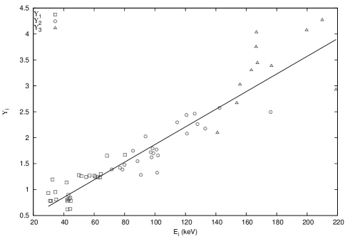
Figure 9: $\Upsilon_{i}$ values versus excitation energy $E_{i}$ relative to the bandhead in each case.

As a final remark, the logarithm of the spectroscopic factor of Eq. (31) can be represented as a function of neutron number, like in Fig. 10. This quantity shows a decreasing trend with the neutron number, meaning that the unquenched potential predicts shorter half-lives for heavier nuclei than what is observed experimentally.

Figure 10: Logarithm of the spectroscopic factor $S$ versus neutron number $N-126$.

IV Conclusions

We analyzed the available experimental data for favored $\alpha$-transitions to rotational bands built upon a single particle angular momentum projection $\Omega\neq\frac{1}{2}$. The nuclear structure was modeled as an odd-nucleon coupled to a coherent state even-even core, the energy levels of each band being fitted through the use of a deformation parameter $d$ and Hamiltonian strength parameter $A_{1}$ that is related to the deformation through a quadratic dependence. $B\left(E2\right)$ values can be predicted using the systematics of the collective effective charge as function of deformation established in Ref. Del15 . In the absence of experimental data that allows the study of the single particle effective charge contribution, it is expected that these predicted values are smaller than what will be observed in reality.

The fine structure of the $\alpha$-emission spectrum was studied using the coupled channels method, through a QQ interaction tweaked by a coupling strength that behaves linearly with respect to the deformation parameter and reduced width for the g.s.$\rightarrow\Omega$ transition. The predicted values of the intensities are in reasonable agreement with experimental data, usually within a factor less than 3. With additional developments in the structure part, it is expected that the model will be useful for the study of the case $\Omega=\frac{1}{2}$ as well.

Table 1: Bandhead spin and parity, deformation and Hamiltonian strength parameters, experimental and predicted excited energy levels, $B(E2)$ values for the transition $\Omega+2\rightarrow\Omega$ for rotational bands in daughter nuclei where favored $\alpha$-transitions occur.

n	$D\left(I\right)$	$\Omega^{\pi}$	$d$	$A_{1}$	$E_{exp}$	$E_{fit}$	$B\left(E2\right)_{\Omega+2\rightarrow\Omega}$
				keV	keV	keV	W.u.
1	Ra${}_{88}^{225}$	5+	3.804	475.876	236.25 3	-	124.244
		7+			267.92 5	285.044
		9+			321.76 8	336.732
		11+			390.0 4	399.098
		13+			487 3	471.662
		15+			-	554.036
		17+			-	645.556
2	Ac${}_{89}^{223}$	5-	2.496	181.721	0	-	49.855
		7-			42.4 1	43.582
		9-			90.7 1	89.180
		11-			141 5	141.602
		13-			-	197.948
		15-			-	260.189
		17-			-	323.633
3	Ac${}_{89}^{225}$	5+	3.066	305.552	155.65 7	-	76.802
		7+			199.85 9	203.667
		9+			257.04 16	255.341
		11+			-	316.518
		13+			-	385.988
		15+			-	463.502
		17+			-	547.239
4	Th${}_{90}^{229}$	5+	3.716	458.930	0	-	117.801
		7+			42.4349 2	49.150
		9+			97.13595 24	101.467
		11+			163.2542 7	164.504
		13+			241.546 19	237.728
		15+			327.8 3	320.725
		17+			-	412.752
5	Th${}_{90}^{231}$	7-	3.589	490.657	387.836 1	-	79.654
		9-			452.176 15	457.046
		11-			530.24 5	528.029
		13-			-	610.351
		15-			-	703.366
		17-			-	806.423
		19-			-	918.846
6	Pa${}_{91}^{231}$	5+	3.984	702.273	183.4962 17	-	138.117
		7+			247.320 5	246.436
		9+			304.5 4	315.768
		11+			406.1 3	399.615
		13+			-	497.451
		15+			-	608.810
		17+			-	732.964
7	Pa${}_{91}^{233}$	5+	3.700	587.036	237.89 13	-	116.653
		7+			300.50 3	298.987
		9+			365.84 8	366.507
		11+			-	447.840
		13+			589 4	542.285
		15+			-	649.306
		17+			-	767.923
n	$D\left(I\right)$	$\Omega^{\pi}$	$d$	$A_{1}$	$E_{exp}$	$E_{fit}$	$B\left(E2\right)_{\Omega+2\rightarrow\Omega}$
				keV	keV	keV	W.u.
8	U ${}_{92}^{237}$	5+	3.775	489.617	159.962 14	-	122.096
		7+			204.17 7	210.550
		9+			260.93 12	264.578
		11+			327.3 10	329.739
		13+			409.8 10	405.515
		15+			501.4 12	491.493
		17+			607.7 12	586.958
9	Np${}_{93}^{235}$	5-	3.824	463.486	49.10 5	-	125.739
		7-			91.6 3	95.349
		9-			146.8 7	145.150
		11-			-	205.255
		13-			-	275.213
		15-			-	354.654
		17-			-	442.954
10	Np${}_{93}^{237}$	5-	3.817	496.159	59.54092 22	-	125.214
		7-			102.959 3	108.698
		9-			158.497 3	162.212
		11-			225.957 16	226.791
		13-			305.050 3	301.948
		15-			395.53 4	387.283
		17-			497.01 5	482.120
11	Np${}_{93}^{239}$	5-	3.738	472.328	74.6640 10	-	119.391
		7-			117.715 40	123.468
		9-			173.086 18	176.660
		11-			241.312 24	240.775
		13-			317.4 15	315.282
		15-			-	399.767
		17-			-	493.493
12	Pu${}_{94}^{239}$	5-	3.704	478.740	285.460 2	-	116.939
		7-			330.124 4	336.658
		9-			387.42 2	391.599
		11-			462 3	457.784
		13-			-	534.646
		15-			-	621.748
		17-			-	718.299
13	Pu${}_{94}^{241}$	7+	3.502	434.114	175.0523 14	-	75.420
		9+			231.935 9	238.742
		11+			301.172 16	304.665
		13+			385 3	380.962
		15+			-	466.987
		17+			-	562.094
		19+			-	665.617
14	Am${}_{95}^{241}$	3-	3.449	432.807	471.812 9	-	141.463
		5-			504.451 9	510.215
		7-			550.4 4	556.342
		9-			625.2 5	616.164
		11-			682.1 6	684.941
		13-			787.2 6	768.880
		15-			863.8 7	856.494
n	$D\left(I\right)$	$\Omega^{\pi}$	$d$	$A_{1}$	$E_{exp}$	$E_{fit}$	$B\left(E2\right)_{\Omega+2\rightarrow\Omega}$
				keV	keV	keV	W.u.
15	Am${}_{95}^{243}$	3-	3.465	409.433	265 10	-	142.950
		5-			300 2	301.257
		7-			345 1	344.467
		9-			-	400.496
		11-			-	464.992
		13-			-	543.654
		15-			-	625.919
16	Am${}_{95}^{245}$	7+	3.389	467.904	327.428 8	-	70.148
		9+			395.870 2	399.236
		11+			475.52 3	475.021
		13+			563.1 3	562.466
		15+			-	660.747
		17+			-	769.069
		19+			-	886.603
17	Cm${}_{96}^{243}$	7+	3.040	281.795	114 20	-	55.439
		9+			164 3	169.285
		11+			228 3	225.576
		13+			-	289.679
		15+			-	360.773
		17+			-	438.184
		19+			-	521.137
18	Cm${}_{96}^{245}$	9-	3.667	395.789	388.181 13	-	63.542
		11-			442.918 21	453.613
		13-			508.87 3	516.475
		15-			587.9 10	587.652
		17-			672 3	666.679
		19-			-	753.084
		21-			-	846.399
19	Cm${}_{96}^{249}$	7+	3.511	460.624	48.76 4	-	75.851
		9+			109.49 9	115.521
		11+			182.77 16	185.116
		13+			268.8 3	265.682
		15+			-	356.540
		17+			-	457.015
		19+			-	566.406
20	Bk${}_{97}^{241}$	3-	3.433	380.147	51 4	-	139.986
		5-			82 6	85.570
		7-			128 7	126.486
		9-			-	179.561
		11-			-	240.500
		13-			-	314.926
		15-			-	392.457
21	Bk${}_{97}^{247}$	3-	3.281	332.176	0	-	126.436
		5-			29.88 11	33.443
		7-			71.60 13	72.792
		9-			125.5 4	123.949
		11-			-	181.849
		13-			-	253.117
		15-			-	325.800
22	Bk${}_{97}^{249}$	7+	3.667	358.729	0	-	83.581
		9+			41.805 8	50.471
		11+			93.759 8	100.203
		13+			155.854 10	157.973
		15+			229.242 12	223.360
		17+			311.857 23	295.932
		19+			-	375.243
n	$D\left(I\right)$	$\Omega^{\pi}$	$d$	$A_{1}$	$E_{exp}$	$E_{fit}$	$B\left(E2\right)_{\Omega+2\rightarrow\Omega}$
				keV	keV	keV	W.u.
23	Bk${}_{97}^{251}$	7+	3.771	312.780	$\sim$35.5	-	89.011
		9+			70 3	78.934
		11+			$\sim$124	119.950
		13+			-	167.687
		15+			-	221.829
		17+			-	282.046
		19+			-	347.998
24	Cf${}_{98}^{247}$	9-	3.600	328.578	480.40 9	-	61.000
		11-			531.99 21	538.111
		13-			595 4	592.167
		15-			-	653.285
		17-			-	721.042
		19-			-	795.013
		21-			-	874.780
25	Cf${}_{98}^{251}$	7+	3.874	565.534	106.309 18	-	94.611
		9+			166.303 23	174.178
		11+			239.33 3	244.459
		13+			325.29 3	326.389
		15+			423.92 4	419.477
		17+			-	523.204
		19+			-	637.027
26	Cf${}_{98}^{253}$	9+	3.274	447.757	241.01 8	-	49.612
		11+			321.21 22	326.500
		13+			417 5	414.539
		15+			-	513.164
		17+			-	621.496
		19+			-	738.703
		21+			-	863.988

Table 2: Sequence of $l$-values that reproduces the fine structure of the emission spectrum, QQ coupling strength between $\alpha$-particle and odd-mass daughter nucleus, Q-value for the g.s.$\rightarrow\textrm{ }\Omega 0$ transition, experimental and predicted logarithm of the total half-life in the $\alpha$-channel, experimental and predicted values for the favored decay intensities to the first three excited states of each rotational band.

n	$D\left(I\right)$	$l_{g.s.\rightarrow\Omega}$	$l_{g.s.\rightarrow\Omega+1}$	$l_{g.s.\rightarrow\Omega+2}$	$l_{g.s.\rightarrow\Omega+3}$	C	$Q_{g.s.\rightarrow\Omega}$	$\log_{10}T_{\alpha}^{exp}$	$\log_{10}T_{\alpha}^{pred}$	$\Upsilon_{1}^{exp}$	$\Upsilon_{1}^{pred}$	$\Upsilon_{2}^{exp}$	$\Upsilon_{2}^{pred}$	$\Upsilon_{3}^{exp}$	$\Upsilon_{3}^{pred}$
								(MeV)	(s)	(s)
1	Ra${}_{88}^{225}$	0	2	3	4	0.107	4.931	11.362	10.477	0.780	0.779	1.748	1.672	2.669	2.820
2	Ac${}_{89}^{223}$	0	1	2	3	0.073	6.580	3.432	1.819	0.620	0.319	1.284	1.287	2.097	2.424
3	Ac${}_{89}^{225}$	0	1	2	3	0.085	5.679	7.433	6.168	0.627	0.342	1.326	1.324	-	2.455
4	Th${}_{90}^{229}$	0	2	3	4	0.133	4.909	12.669	11.677	0.810	0.809	1.720	1.720	3.301	2.795
5	Th${}_{90}^{231}$	0	2	3	4	0.112	4.290	16.342	16.291	1.301	1.301	2.574	2.402	-	3.990
6	Pa${}_{91}^{231}$	0	2	3	4	0.052	5.011	12.117	11.392	1.234	1.231	2.079	2.124	-	3.815
7	Pa${}_{91}^{233}$	0	2	3	4	0.061	4.720	13.833	13.394	1.238	1.238	2.262	2.226	-	3.804
8	U ${}_{92}^{237}$	0	2	3	4	0.114	4.980	13.264	12.095	0.840	0.841	1.773	1.747	3.442	2.847
9	Np${}_{93}^{235}$	0	2	3	4	0.107	5.874	8.633	7.206	0.778	0.777	1.623	1.589	-	2.552
10	Np${}_{93}^{237}$	0	2	3	4	0.104	5.578	10.146	8.831	0.815	0.814	1.699	1.647	3.753	2.714
11	Np${}_{93}^{239}$	0	2	3	4	0.083	5.364	11.362	10.046	0.898	0.898	1.793	1.736	4.036	2.932
12	Pu${}_{94}^{239}$	0	2	3	4	0.115	5.883	8.964	7.583	0.784	0.783	1.659	1.599	3.386	2.656
13	Pu${}_{94}^{241}$	0	2	3	4	0.069	5.447	11.431	9.997	1.270	1.267	2.463	2.114	4.270	3.736
14	Am${}_{95}^{241}$	0	2	2	4	0.033	5.983	8.554	7.337	1.196	1.201	1.388	1.170	-	3.789
15	Am${}_{95}^{243}$	0	2	3	4	0.061	5.623	10.643	9.447	0.808	0.811	1.477	1.639	-	2.799
16	Am${}_{95}^{245}$	0	2	3	4	0.042	5.198	12.286	11.997	1.653	1.655	-	2.656	-	4.669
17	Cm${}_{96}^{243}$	0	2	3	4	0.070	6.400	7.505	5.699	1.279	1.283	-	2.003	-	3.587
18	Cm${}_{96}^{245}$	0	2	3	4	0.093	5.908	10.041	8.278	1.242	1.241	2.437	1.956	4.075	3.477
19	Cm${}_{96}^{249}$	0	2	3	4	0.065	6.077	8.696	7.274	1.253	1.250	-	2.055	-	3.625
20	Bk${}_{97}^{241}$	0	2	3	4	0.052	7.858	2.217	0.125	0.784	0.786	1.421	1.524	-	2.624
21	Bk${}_{97}^{247}$	0	2	3	4	0.042	6.597	7.079	5.161	0.935	0.930	1.390	1.703	-	3.008
22	Bk${}_{97}^{249}$	0	2	3	4	0.055	6.739	6.255	4.486	1.135	1.136	2.025	1.978	3.025	3.179
23	Bk${}_{97}^{251}$	0	2	3	4	0.078	6.401	7.929	6.095	0.953	0.952	1.547	1.639	-	2.727
24	Cf${}_{98}^{247}$	0	2	3	4	0.075	6.945	5.978	4.061	1.258	1.259	2.296	1.900	-	3.339
25	Cf${}_{98}^{251}$	0	2	3	4	0.044	7.133	4.857	3.161	1.270	1.265	2.176	2.020	2.927	3.553
26	Cf${}_{98}^{253}$	0	2	3	4	0.059	6.622	6.940	5.382	1.672	1.674	2.496	2.554	-	4.528