Inflaton decay and reheating in nonminimal derivative coupling

Abstract

We investigate the inflaton decay and reheating period after the end of inflation in the non-minimal derivative coupling (NDC) model with chaotic potential. In general, this model is known to provide an enhanced slow-roll inflation caused by gravitationally enhanced friction. We find violent oscillations of Hubble parameter which induces oscillations of the sound speed squared, implying the Lagrangian instability of curvature perturbation $\zeta$ under the comoving gauge $\varphi=0$. Also, it is shown that the curvature perturbation blows up at $\dot{\phi}=0$, leading to the breakdown of the comoving gauge at $\dot{\phi}=0$. Therefore, we use the Newtonian gauge to perform the perturbation analysis where the Newtonian potential is employed as a physical variable. The curvature perturbation is not considered as a physical variable which describes a relevant perturbation during reheating.

1 Introduction

It is known that reheating is a crucial epoch which connects inflation to the hot big-bang phase [1]. This era is conceptually very important, but it is observationally poorly known. The physics of this phase transition is thought to be highly non-linear [2]. Also, the physics of reheating has turned out to be very complicated [3, 4, 5, 6]. Since the first CMB constraints have performed on the reheating temperature by the WMAP7 [7], the current Planck satellite measurements of the CMB anisotropy constrain the kinematic properties of the reheating era for almost 200 of the inflationary models [8].

The nonminimal derivative coupling (NDC) [9, 10] was made by coupling the inflaton kinetic term to the Einstein tensor such that the friction is enhanced gravitationally [11]. The gravitationally enhanced friction mechanism has been considered as an alternative to increase friction of an inflaton rolling down its own potential. Actually, the NDC makes a steep (non-flat) potential adequate for inflation without introducing higher-time derivative terms (ghost state) [12, 13]. This implies that the NDC increases friction and thus, it flattens the potential effectively.

It is worth to note that there was a difference in whole dynamics between canonical coupling (CC) and NDC even for taking the same potential [14]. A clear difference appears after the end of inflation. We note that there are three phases in the CC case [15]: i) Initially, kinetic energy dominates. ii) Due to the rapid decrease of the kinetic energy, the trajectory runs into the inflationary attractor line (potential energy dominated). All initial trajectories are attracted to this line, which is the key feature of slow-roll inflation. iii) At the end of inflation, the inflaton velocity decreases. Then, there is inflaton decay and reheating [the appearance of spiral sink in the phase portrait $(\phi,\dot{\phi})$].

On the other hand, three stages of NDC are as follows: i) Initially, potential energy dominates. ii) Due to the gravitationally enhanced friction (restriction on inflaton velocity $\dot{\phi}$), all initial trajectories are attracted quickly to the inflationary attractor. iii) At the end of inflation, the inflaton velocity increases. Then, there is inflaton decay and followed by reheating. Importantly, there exist oscillations of inflaton velocity without damping due to violent oscillations of Hubble parameter. This provides stable limited cycles in the phase portrait $(\phi,\dot{\phi})$, instead of spiral sink in CC. However, it was shown that analytic expressions for inflaton and Hubble parameter after the inflation could be found by applying the averaging method to the NDC [16]. The inflaton oscillates with time-dependent frequency, while the Hubble parameter does not oscillate. Introducing an interacting Lagrangian of ${\cal L}_{\rm int}=-\frac{1}{2}g^{2}\phi^{2}\chi^{2}$, they have claimed that the parametric resonance instability is absent, implying a crucial difference when comparing to the CC. This requires a complete solution by solving NDC-equations numerically. Recently, the authors in [17] have investigated particle production after inflation by considering the combined model of CC+NDC. They have insisted that the violent oscillation of Hubble parameter causes particle production even though the Lagrangian instability appears due to oscillations of the sound speed squared $c_{s}^{2}$ which also appeared in the generalized Galilean theory [18].

One usually assumes that the field mode is frozen (time-independent) at late time after entering into the super-horizon. Therefore, it was accepted that the perturbation during the reheating is less important than that of inflation. However, in exploring the effects of reheating on the cosmological perturbations of CC case, one has to face the breakdown of the curvature perturbation $\zeta$ at $\dot{\phi}=0$ when choosing the comoving gauge of $\varphi=0$. This issue may be bypassed by replacing $\dot{\phi}^{2}$ by its time average $\langle\dot{\phi}^{2}\rangle$ over the inflaton oscillation [19, 20, 21]. Recently, it was proposed that the breakdown of the comoving gauge $\varphi=0$ at $\dot{\phi}=0$ could be resolved by introducing the $cd$-gauge which eliminates $\varphi$ in the Hamiltonian formalism of the CC model and thus, provides a well-behaved curvature perturbation $\zeta$ [22]. However, it turned out that choosing the Newtonian gauge is necessary to study the perturbation during the oscillating period, since the comoving gauge is not suitable for performing the perturbation analysis during the reheating [23].

In this work, we find a complete solution for inflaton and Hubble parameter by solving the NDC-equations numerically in Section 2. The NDC model may be dangerous because the inflaton becomes strongly coupled when the Hubble parameter tends towards zero. Hence, we wish to obtain a complete solution for inflaton and Hubble parameter by solving the CC+NDC-equations numerically in Section 3. Here, we can control mutual importance of the CC and NDC by adjusting two coefficients. In Section 4, we will investigate the curvature perturbation $\zeta$ during reheating by considering the NDC with the chaotic potential and choosing the comoving gauge. We find that violent oscillations of Hubble parameter induce oscillations of the sound speed squared, implying the Lagrangian instability of curvature perturbation. More seriously, we show that the curvature perturbation blows up at $\dot{\phi}=0$, implying that the curvature perturbation is ill-defined under the comoving gauge of $\varphi=0$. This suggests a different gauge without problems at $\dot{\phi}=0$. Hence, we choose the Newtonian gauge to perform the perturbation analysis where the Newtonian potential is considered as a physical variable in Section 5.

2 NDC with chaotic potential

We introduce an inflation model including the NDC of scalar field $\phi$ with the chaotic potential [24, 14]

$$S=\frac{1}{2}\int d^{4}x\sqrt{-g}\Big{[}M_{\rm P}^{2}R+\frac{1}{\tilde{M}^{2}}G_{\mu\nu}\partial^{\mu}\phi\partial^{\nu}\phi-2V(\phi)\Big{]},~{}~{}V=V_{0}\phi^{2},$$ (2.1)

where $M_{\rm P}$ is a reduced Planck mass, $\tilde{M}$ is a mass parameter and $G_{\mu\nu}$ is the Einstein tensor. Here, we do not include a canonical coupling (CC) term like as a conventional combination of CC+NDC [$(g_{\mu\nu}-G_{\mu\nu}/\tilde{M}^{2})\partial^{\mu}\phi\partial^{\nu}\phi$] [25, 26] because this combination won’t make the whole analysis transparent.

From the action (2.1), we derive the Einstein and inflaton equations

$$G_{\mu\nu}=\frac{1}{M_{\rm P}^{2}}T_{\mu\nu},$$ (2.2)

$$\frac{1}{\tilde{M}^{2}}G^{\mu\nu}\nabla_{\mu}\nabla_{\nu}\phi+V^{\prime}=0,$$ (2.3)

where $T_{\mu\nu}$ takes a complicated form

$$T_{\mu\nu} = \frac{1}{\tilde{M}^{2}}\Big{[}\frac{1}{2}R\nabla_{\mu}\phi\nabla_{\nu}\phi-2\nabla_{\rho}\phi\nabla_{(\mu}\phi R_{\nu)}^{\rho}+\frac{1}{2}G_{\mu\nu}(\nabla\phi)^{2}-R_{\mu\rho\nu\sigma}\nabla^{\rho}\phi\nabla^{\sigma}\phi$$ (2.4)

$$\hskip 50.00008pt-\nabla_{\mu}\nabla^{\rho}\phi\nabla_{\nu}\nabla_{\rho}\phi+(\nabla_{\mu}\nabla_{\nu}\phi)\nabla^{2}\phi$$

$$-g_{\mu\nu}\Big{(}-R^{\rho\sigma}\nabla_{\rho}\phi\nabla_{\sigma}\phi+\frac{1}{2}(\nabla^{2}\phi)^{2}-\frac{1}{2}(\nabla^{\rho}\nabla^{\sigma}\phi)\nabla_{\rho}\nabla_{\sigma}\phi\Big{)}\Big{]}.$$

Considering a flat FRW spacetime by introducing cosmic time $t$ as

$$ds^{2}_{\rm FRW}~{}=~{}\bar{g}_{\mu\nu}dx^{\mu}dx^{\nu}~{}=~{}-dt^{2}+a^{2}(t)\delta_{ij}dx^{i}dx^{j},$$ (2.5)

two Friedmann and inflaton equations (NDC-equations) derived from (2.2) and (2.3) are given by

$$H^{2} = \frac{1}{3M_{\rm P}^{2}}\Big{[}\frac{9H^{2}}{2\tilde{M}^{2}}\dot{\phi}^{2}+V\Big{]},$$ (2.6)

$$\dot{H} = -\frac{1}{2M_{\rm P}^{2}}\Big{[}\dot{\phi}^{2}\Big{(}\frac{3H^{2}}{\tilde{M}^{2}}-\frac{\dot{H}}{\tilde{M}^{2}}\Big{)}-\frac{2H}{\tilde{M}^{2}}\dot{\phi}\ddot{\phi}\Big{]},$$ (2.8)

$$\frac{3H^{2}}{\tilde{M}^{2}}\ddot{\phi}+3H\Big{(}\frac{3H^{2}}{\tilde{M}^{2}}+\frac{2\dot{H}}{\tilde{M}^{2}}\Big{)}\dot{\phi}+V^{\prime}=0.$$

Here $H=\dot{a}/a$ is the Hubble parameter and the overdot ($\dot{}$) denotes derivative with respect to time $t$. It is evident from (2.6) that the energy density for the NDC is positive (ghost-free).

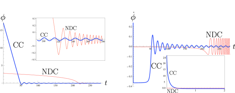
Figure 1: The whole evolution of $\phi(t)$ [left] and $\dot{\phi}(t)$ [right] with respect to time $t$ for chaotic potential $V=V_{0}\phi^{2}$ with $V_{0}=0.1$. The left figure shows that the inflaton varies little during large inflationary period ($0\leq t\leq 200$) for the NDC, while it varies quickly during small inflationary period ($0\leq t\leq 45$) for the CC. After inflation (see figure in box), $\phi$ decays with oscillation for CC, while it oscillates rapidly for NDC. The right one indicates that for large $t$, $\dot{\phi}$ oscillates without damping for NDC, while it oscillates with damping for the CC. Figure in box shows initially kinetic energy phase for CC and initially potential phase for NDC.

At this stage, the CC model of $-g_{\mu\nu}\partial^{\mu}\phi\partial^{\nu}\phi$ is introduced to compare with the NDC case. In this case, the CC-equations are given by

$$H^{2} = \frac{1}{3M_{\rm P}^{2}}\Big{[}\frac{1}{2}\dot{\phi}^{2}+V\Big{]},$$ (2.9)

$$\dot{H} = -\frac{1}{2M_{\rm P}^{2}}\dot{\phi}^{2},$$ (2.10)

$$\ddot{\phi} + 3H\dot{\phi}+m^{2}\phi=0$$ (2.11)

with $m^{2}=2V_{0}$. Fig. 1 shows a whole evolution of $\phi$ and $\dot{\phi}$ based on numerical computation. When the universe evolves according to (2.9)-(2.11), there are three phases in the CC case [15]: i) Initially, kinetic energy dominates [see Fig. 1 (right)]. ii) Due to the rapid decrease of the kinetic energy, the trajectory runs quickly to the inflationary attractor line. All initial trajectories are attracted to this line, which is the key feature of slow-roll inflation. iii) Finally, after the end of inflation, there is inflaton decay and reheating which corresponds to spiral sink in the phase portrait ($\phi,\dot{\phi}$). Explicitly, (2.9) can be parameterized by using the Hubble parameter $H$ and the angular variable $\theta$ as

$$\dot{\phi} = \sqrt{6}HM_{\rm P}\cos\theta,$$ (2.12)

$$m\phi = \sqrt{6}HM_{\rm P}\sin\theta,$$ (2.13)

while (2.10) and (2.11) implies

$$\dot{H} = -3H^{2}\cos^{2}\theta,$$ (2.14)

$$\dot{\theta} = -m-\frac{3}{2}H\sin(2\theta).$$ (2.15)

For $m\gg H$, (2.15) reduces to $\dot{\theta}\simeq-m$ which implies a solution of $\theta\simeq-mt$. Plugging the latter into (2.13) indicates that $\phi$ oscillates with frequency $\omega\simeq m=0.45$ for $V_{0}=0.1$. Solving (2.14) leads to

$$H(t)\simeq\frac{2}{3t}\Big{[}1+\frac{\sin(2mt)}{2mt}\Big{]}^{-1}$$ (2.16)

which shows small oscillations around $\frac{2}{3t}$. Actually, its time rate is given by

$$\dot{H}(t)\simeq-\frac{16m^{2}\cos^{2}(mt)}{3\Big{[}2mt+\sin(2mt)\Big{]}^{2}}=-\frac{8m^{2}[1+\cos(2mt)]}{3\Big{[}2mt+\sin(2mt)\Big{]}^{2}}$$ (2.17)

whose amplitude approaches zero ($-\frac{2}{3t^{2}}$) with oscillations as $t$ increases. Its frequency is given by $\omega^{\rm CC}_{\dot{H}}=2m$. Substituting (2.16) into (2.13) provides us the scalar

$$\phi(t)\simeq\sqrt{\frac{8}{3}}\frac{M_{\rm P}}{mt}\sin(mt)\Bigg{[}1-\frac{\sin(2mt)}{2mt}\Bigg{]},$$ (2.18)

which implies that after the end of inflation, the friction becomes subdominant and thus, $\phi(t)$ becomes an oscillator whose amplitude gets damped due to the universe evolution $H$. The time rate is given by

$$\dot{\phi}(t)\simeq\sqrt{\frac{8}{3}}\frac{M_{\rm P}}{t}\cos(mt)\Bigg{[}1-\frac{\sin(2mt)}{2mt}\Bigg{]}.$$ (2.19)

We observe that $\omega^{\rm CC}_{\phi}=\omega^{\rm CC}_{\dot{\phi}}=m$.

The scale factor can be extracted from (2.16) as

$$a(t)\simeq t^{\frac{2}{3}},$$ (2.20)

while the energy density of $\phi$ decreases in the same way as the energy density of non-relativistic particles of mass $m$

$$\rho_{\phi}=\frac{1}{2}\Big{[}\dot{\phi}^{2}+m^{2}\phi^{2}\Big{]}\sim\frac{1}{a^{3}}.$$ (2.21)

This indicates that the inflaton oscillations can be interpreted to be a collection of scalar particles, which are independent from each other, oscillating coherently at the same frequency $m$.

Differing with the CC model, the upper limit of $\dot{\phi}^{2}$ is set for the NDC model

$$0<\dot{\phi}^{2}\leq\phi_{c}^{2}\equiv\frac{2}{3}M_{\rm P}^{2}\tilde{M}^{2},$$ (2.22)

which comes from Eq.(2.6) showing that $3M^{2}_{\rm P}H^{2}(1-\dot{\phi}^{2}/\phi^{2}_{c})=V\geq 0$. Based on (2.6)-(2.8), we can figure out a whole picture numerically [see Fig.1 (left)]. Three stages are in the NDC: i) Initially, potential energy dominates. ii) Due to the gravitationally enhanced friction, all initial trajectories are attracted quickly to the inflationary attractor. iii) At the end of inflation, the inflaton velocity increases. Then, there is inflaton decay and followed by reheating. However, there exist oscillations of inflaton velocity without damping. This provides stable limited cycles in the phase portrait $(\phi,\dot{\phi})$, instead of spiral sink. We stress that an analytic solution for NDC is not yet known because equations (2.6)-(2.8) are too complicated to be solved. However, the would-be analytic solution might be found in [16].

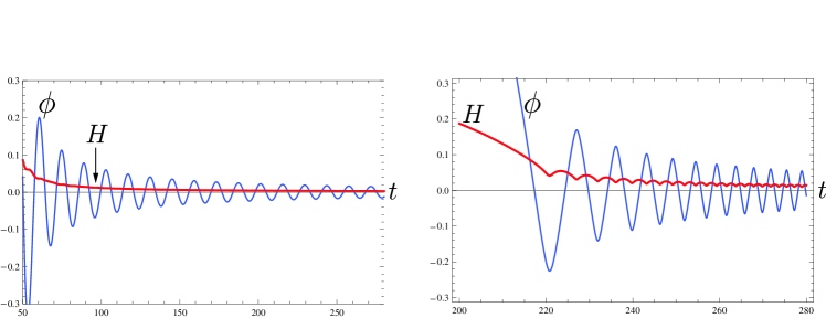
Figure 2: After the end of inflation, behaviors of inflation $\phi$ (blue) and Hubble parameter $H$ (red) with respect to time $t$. Left picture is for CC while right one represents the NDC case. We observe violent oscillations of $H$ for NDC. Here, angular frequency of $H$ is given by $\omega_{H}(t)=2\omega_{\phi}(t)$ for NDC, while frequency of $\phi$ is $\omega^{\rm CC}_{\phi}=m$ for CC.

Now we are in a position to focus on the reheating period after the end of inflation (post-inflationary phase). We remind the reader that the friction term dominates in the slow-roll inflation period, while the friction term becomes subdominant in the reheating process. Therefore, the inflaton becomes an oscillator whose amplitude gets damped due to the universe expansion. Fig. 2 shows behaviors of inflation $\phi$ and Hubble parameter $H$ with respect to time $t$. Left figure is designed for CC [(2.18) and (2.16)], while the right one represents the NDC case. We observe violent oscillations of $H$ for NDC. Here, oscillation frequency of $H$ is given by $\omega_{H}(t)=2\omega_{\phi}(t)$ for NDC. Fig. 3 indicates behaviors of inflaton velocity $\dot{\phi}$ (blue) and Hubble parameter $H$ (red) with respect to time $t$. Left picture is for CC [(2.19) and (2.16)], while the right one represents the NDC case. We find violent oscillations of $H$ for NDC. Here, oscillation frequency of $H$ is still given by $\omega_{H}(t)=2\omega_{\dot{\phi}}(t)$ for NDC. Importantly, we observe a sizable difference that $\dot{\phi}$ oscillates with damping (CC), while it oscillates without damping and its frequency increases (NDC).

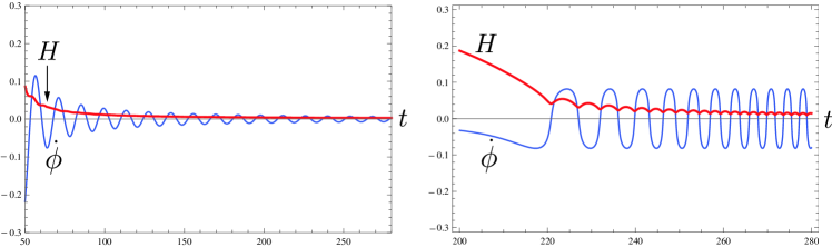
Figure 3: After the end of inflation, behaviors of inflaton velocity $\dot{\phi}$ (blue) and Hubble parameter $H$ (red) with respect to time $t$. Left picture is for CC, while right one represents the NDC case. We observe violent oscillations of $H$ for NDC. Oscillation frequency of $H$ is given by $\omega_{H}(t)=2\omega_{\dot{\phi}}(t)$ for NDC, while the frequency of $\dot{\phi}$ is $\omega^{\rm CC}_{\dot{\phi}}=m$ for CC.

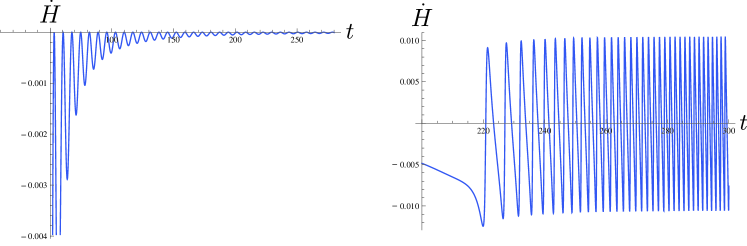
Figure 4: Oscillations of $\dot{H}$ after the end of inflation: Left (CC) and Right (NDC). Here we observe the difference between CC and NDC: $\dot{H}\leq 0$ for CC and $-0.01\leq\dot{H}\leq 0.01$.

Here, we mention that different behaviors of $\phi$ and $\dot{\phi}$ between CC and NDC have arisen from different oscillations of their Hubble parameter $H$. Their change of rates $\dot{H}$ are depicted in Fig. 4, which would be used to obtain the sound speed squared $c^{2}_{s}$. It is quite interesting to note the difference that $\dot{H}$ of CC [(2.17)] approaches zero (along $-\frac{2}{3t^{2}}$) with oscillations ($\omega^{\rm CC}_{\dot{H}}=2m$), while $\dot{H}$ oscillates between $-0.01$ and 0.01 with frequency $\omega_{\dot{H}}(t)$.

At this stage, we note that an analytic solution might be obtained by using the averaging method [16]. This is given by

$$H_{\rm a}(t)=\frac{2}{3(2-\sqrt{2})t},$$ (2.23)

$$\phi_{\rm a}(t)=\frac{\sqrt{6}M_{\rm P}H_{\rm a}(t)}{m}\cos\Big{[}\frac{m\tilde{M}}{2}(2-\sqrt{2})(\sqrt{2}-\frac{1}{2})t^{2}\Big{]},$$ (2.24)

where $\phi_{\rm a}(t)$ oscillates with time-dependent frequency. Their time-rates are given by

$$\dot{H}_{\rm a}(t)=-\frac{2}{3(2-\sqrt{2})t^{2}},$$ (2.25)

$$\dot{\phi}_{\rm a}(t)=-\frac{(4-\sqrt{2})M_{\rm P}\tilde{M}}{\sqrt{3}}\sin\Big{[}\frac{m\tilde{M}}{2}(2-\sqrt{2})(\sqrt{2}-\frac{1}{2})t^{2}\Big{]}+\cdots.$$ (2.26)

We wish to comment here that even though $\dot{\phi}_{\rm a}(t)$ could mimic $\dot{\phi}$ in the right picture of Fig. 3, $\dot{H}_{\rm a}(t)$ could not describe oscillations of $\dot{H}$ in the right-picture of Fig. 4. This implies that the analytic solution (2.23) is not a proper solution to NDC-equations because $H_{\rm a}(t)$ did not show violent oscillations of Hubble parameter. Also we observe the difference in frequency between CC and NDC: $\omega^{\rm CC}_{\phi}=\omega^{\rm CC}_{\dot{\phi}}=m$, $\omega^{\rm CC}_{\dot{H}}=2m$ (time-independent) and $\omega_{H}(t)=2\omega_{\phi}=2\omega_{\dot{\phi}}$, $\omega_{\dot{H}}(t)$(time-dependent).

Hence, it is not proven that the parametric resonance is absent for NDC when considering the decay of inflaton into a relativistic field (${\cal L}_{\rm int}=-\frac{1}{2}g^{2}\phi^{2}\chi^{2}$), whereas the parametric resonance is present for CC.

3 CC + NDC with chaotic potential

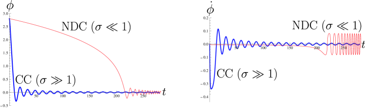
Figure 5: The whole evolution of $\phi(t)$ [left] and $\dot{\phi}(t)$ [right] with respect to time $t$ for chaotic potential $V=V_{0}\phi^{2}$ with $V_{0}=0.1$. In these figures, CC-dominant (blue) and NDC-dominant (red) cases correspond to $\sigma=10^{4}\gg 1$ and $\sigma=10^{-4}\ll 1$, respectively.

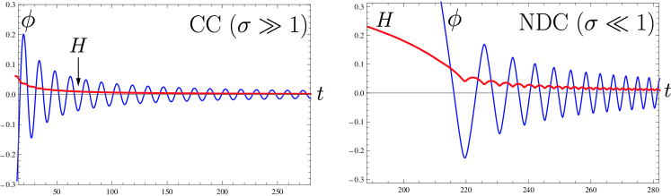
Figure 6: After the end of inflation, behaviors of inflaton $\phi$ (blue) and Hubble parameter $H$ (red) with respect to time $t$. Left picture is for CC-dominant case ($\sigma=10^{4}\gg 1$), while right one represents the NDC-dominant ($\sigma=10^{-4}\ll 1$) case.

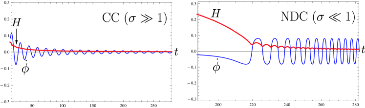
Figure 7: After the end of inflation, behaviors of inflaton velocity $\dot{\phi}$ (blue) and Hubble parameter $H$ (red). Left picture is for CC-diminant case ($\sigma=10^{4}\gg 1$), while right one represents the NDC-dominant ($\sigma=10^{-4}\ll 1$) case.

In this section, we wish to study the homogeneous evolution of the CC$+$NDC model. It is noted that the NDC (2.1) without CC term might be dangerous when the Hubble parameter tends to zero. That is, tending of Hubble parameter to zero may induce a strongly coupled inflaton. To this end, we start with the CC$+$NDC action with chaotic potential as

$$S_{\rm CC+NDC}=\frac{1}{2}\int d^{4}x\sqrt{-g}\Big{[}M_{\rm P}^{2}R-\Big{(}\sigma_{\rm C}g_{\mu\nu}-\sigma_{\rm N}G_{\mu\nu}\Big{)}\partial^{\mu}\phi\partial^{\nu}\phi-2V(\phi)\Big{]},~{}V=V_{0}\phi^{2}.$$ (3.1)

The CC$+$NDC-equations are given by

$$H^{2} = \frac{1}{3M_{\rm P}^{2}}\Big{[}\frac{1}{2}(\sigma_{\rm C}+9H^{2}\sigma_{\rm N})\dot{\phi}^{2}+V\Big{]},$$ (3.2)

$$\dot{H} = -\frac{1}{2M_{\rm P}^{2}}\Big{[}\dot{\phi}^{2}(\sigma_{\rm C}+3H^{2}\sigma_{\rm N}-\dot{H}\sigma_{\rm N})-2H\sigma_{\rm N}\dot{\phi}\ddot{\phi}\Big{]},$$ (3.4)

$$(\sigma_{\rm C}+3H^{2}\sigma_{\rm N})\ddot{\phi}+3H(\sigma_{\rm C}+3H^{2}\sigma_{\rm N}+2\dot{H}\sigma_{\rm N})\dot{\phi}+V^{\prime}=0,$$

where $\sigma_{\rm N}=1/\tilde{M}^{2}$ and $\sigma_{\rm C}$ is introduced to denote a new coefficient for the CC term.

Now we can solve Eqs.(3.2)-(3.4) numerically. Denoting $\sigma\equiv\sigma_{\rm C}/\sigma_{\rm N}$, we obtain the CC-dominant case by taking $\sigma\gg 1$ and the NDC-dominant case by taking $\sigma\ll 1$. Fig. 5 shows the whole evolution of $\phi$ (left) and $\dot{\phi}$ (right), while Fig. 6 and 7 indicate the evolution after the end of inflation for ($\phi,H)$ and ($\dot{\phi},H)$, respectively. Also, after the end of inflation, $\dot{H}(t)$ is depicted in Fig. 8.

Importantly, we note that the evolutions given in Fig. 1-4 correspond to those in Fig. 5-8, respectively. We observe that they are very similar to each other. Therefore, it is clear that the evolution of the NDC-equations (2.6)-(2.8) could be recovered from the NDC-dominant case of the CC$+$NDC-equations (3.2)-(3.4), while the CC-equations (2.9)-(2.11) could be recovered from the CC-dominant case of the CC$+$NDC-equations.

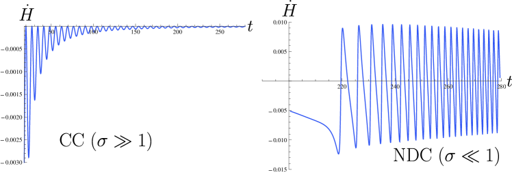
Figure 8: Oscillations of $\dot{H}$ after the end of inflation: Left (CC-dominance: $\sigma=10^{4}\gg 1$) and right (NDC-dominance: $\sigma=10^{-4}\ll 1$).

4 Curvature perturbation in the comoving gauge

In order to find what happens in the post-inflationary phase, it would be better to analyze the perturbation. We use the ADM formalism to resolve the mixing between scalar of metric and inflaton

$$ds_{\rm ADM}^{2}=-N^{2}dt^{2}+\gamma_{ij}(dx^{i}+\beta^{i}dt)(dx^{j}+\beta^{j}dt),$$ (4.1)

where $N$, $\beta_{i}$, and $\gamma_{ij}$ denote lapse, shift vector, and spatial metric tensor. In this case, the action (2.1) can be written as

$$S=\int d^{4}x\sqrt{-g}\Big{[}\frac{M_{\rm P}^{2}}{2}R+\frac{G^{00}}{\tilde{M}^{2}}\frac{\dot{\phi}^{2}}{2}-V\Big{]},$$ (4.2)

where

$$R = R^{(3)}+\frac{1}{N^{2}}(E^{ij}E_{ij}-E^{2})-2\nabla_{\mu}(Kn^{\mu})-\frac{2}{N}\Delta^{(3)}N,$$ (4.3)

$$G^{00} = \frac{1}{2N^{2}}\Big{[}R^{(3)}+\frac{1}{N^{2}}(E^{2}-E^{ij}E_{ij})\Big{]}.$$ (4.4)

Here $E_{ij}$ is related to the extrinsic curvature $K_{ij}$ and $n^{\mu}$ is the unit normal vector of the timelike hypersurface as

$$E_{ij}=NK_{ij}=\frac{1}{2}(\nabla_{i}^{(3)}\beta_{j}+\nabla_{j}^{(3)}\beta_{i}-\dot{\gamma}_{ij}),~{}~{}n^{\mu}=\frac{1}{N}(1,-\beta^{i}).$$ (4.5)

Then, we express the action (4.2) as

$$S = \frac{M_{\rm P}^{2}}{2}\int d^{4}x\sqrt{\gamma}\Big{[}R^{(3)}\Big{(}N+\frac{\dot{\phi}^{2}}{2NM_{\rm P}^{2}\tilde{M}^{2}}\Big{)}$$ (4.6)

$$\hskip 50.00008pt+(E^{ij}E_{ij}-E^{2})\Big{(}\frac{1}{N}-\frac{\dot{\phi}^{2}}{2N^{3}M_{\rm P}^{2}\tilde{M}^{2}}\Big{)}-\frac{2NV}{M_{\rm P}^{2}}\Big{]}.$$

Varying (4.6) with respect to $N$ and $\beta_{j}$ lead to two constraints

$$R^{(3)}\Big{(}1-\frac{\dot{\phi}^{2}}{2N^{2}M_{\rm P}^{2}\tilde{M}^{2}}\Big{)}-(E^{ij}E_{ij}-E^{2})\Big{(}\frac{1}{N^{2}}-\frac{3\dot{\phi}^{2}}{2N^{4}M_{\rm P}^{2}\tilde{M}^{2}}\Big{)}-\frac{2V}{M_{\rm P}^{2}}=0,$$ (4.7)

$$\hskip 100.00015pt\nabla_{i}^{(3)}\Big{[}\Big{(}\frac{1}{N}-\frac{\dot{\phi}^{2}}{2N^{3}M_{\rm P}^{2}\tilde{M}^{2}}\Big{)}(E^{i}_{j}-\delta^{i}_{j}E)\Big{]}=0.$$ (4.8)

Hereafter, we choose the comoving gauge for the inflaton ($\phi=\phi(t)+\varphi$)

$$\varphi=0.$$ (4.9)

For simplicity, we consider the scalar perturbations

$$N=1+\alpha,~{}\beta_{i}=\partial_{i}\psi,~{}\gamma_{ij}=a^{2}e^{2\zeta}\delta_{ij},$$ (4.10)

where $\zeta$ denotes the curvature perturbation. Solving (4.7) and (4.8), we find the perturbed relations

$$\alpha=\frac{A_{1}}{H}\dot{\zeta},~{}~{}\psi=-\frac{A_{1}}{H}\zeta+\chi,~{}~{}\partial_{i}^{2}\chi=\frac{a^{2}}{H^{2}}\frac{A_{1}^{2}A_{2}}{1-\epsilon_{N}^{H}/3}\dot{\zeta},$$ (4.11)

where $A_{1,2}$ and a slow-roll parameter $\epsilon_{N}^{H}$ are given by

$$A_{1}=\frac{1-\epsilon_{N}^{H}/3}{1-\epsilon_{N}^{H}},~{}~{}A_{2}=\frac{\epsilon_{N}^{H}H^{2}(1+\epsilon_{N}^{H})}{1-\epsilon_{N}^{H}/3},~{}~{}\epsilon_{N}^{H}=\frac{3\dot{\phi}^{2}}{2M_{\rm P}^{2}\tilde{M}^{2}}.$$ (4.12)

Now we wish to expand (4.6) to second order to obtain its bilinear action. Making some integration by parts, we find the bilinear action for $\zeta$ as

$$\delta S_{(2)}=M_{\rm P}^{2}\int d^{4}xa^{3}\frac{A_{1}^{2}A_{2}}{H^{2}}\Big{[}\dot{\zeta}^{2}-\frac{c_{s}^{2}}{a^{2}}(\partial_{i}\zeta)^{2}\Big{]}.$$ (4.13)

Here the sound speed squared $c_{s}^{2}$ is given by

$$c_{s}^{2} = \frac{H^{2}}{A_{1}^{2}A_{2}}A_{3}$$ (4.14)

$$= 1+\frac{4}{9A_{1}}\frac{\epsilon_{N}^{H}}{1+\epsilon_{N}^{H}}+\frac{2\dot{H}}{H^{2}}\frac{1-\epsilon_{N}^{H}/3}{1+\epsilon_{N}^{H}}$$ (4.15)

with

$$A_{3}=\frac{d}{adt}\Big{[}\frac{aA_{1}}{H}\Big{(}1-\frac{\epsilon_{N}^{H}}{3}\Big{)}\Big{]}-1-\frac{\epsilon_{N}^{H}}{3}.$$ (4.16)

We have $A_{1}^{2}A_{2}/H^{2}\geq 0$, which means ghost-free. Unfortunately, we find from Fig. 9 that $c_{s}^{2}$ (NDC) oscillates increasingly after the end of inflation, while it is constant for CC. The former has arisen from the presence of $\dot{H}$ in (4.15) and it may induce the Lagrangian instability (gradient instability) which leads to the fact that the curvature perturbation $\zeta$ grows violently [17].

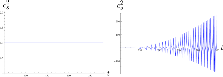
Figure 9: Sound speed squared $c_{s}^{2}$ for curvature perturbation $\zeta$ after the end of inflation: Left (CC) is constant and right (NDC) oscillates increasingly after the end of inflation.

On the other hand, it is known that in CC case, the curvature perturbation $\zeta$ diverges during reheating when $\dot{\phi}=0$ [19, 20, 21]. Furthermore, it is apparent that in NDC case, $\zeta$ is divergent when $\dot{\phi}=\pm\phi_{c}$ [$\epsilon_{N}^{H}=1$] as well as $\dot{\phi}=0$ [$\epsilon_{N}^{H}=0$] during reheating. To see this more closely, we write equation of $\zeta$ from the action (4.13) as

$$\ddot{\zeta}+[3H+F(\epsilon_{N}^{H})]\dot{\zeta}-\frac{c_{s}^{2}}{a^{2}}\partial^{2}\zeta=0,$$ (4.17)

where

$$F(\epsilon_{N}^{H})=\frac{\dot{\epsilon}_{N}^{H}}{\epsilon_{N}^{H}}\times\frac{(\epsilon_{N}^{H})^{3}-3(\epsilon_{N}^{H})^{2}+7\epsilon_{N}^{H}+3}{(\epsilon_{N}^{H}+1)(\epsilon_{N}^{H}-1)(\epsilon_{N}^{H}-3)}.$$ (4.18)

We observe that $F$ behaves as

$$F\simeq\left\{\begin{array}[]{ll}\frac{1}{\epsilon_{N}^{H}}\simeq\frac{1}{\dot{\phi}^{2}},~{}~{}({\rm at}~{}\dot{\phi}=0)\\ \frac{1}{\epsilon_{N}^{H}-1}\simeq\frac{1}{\dot{\phi}^{2}-\phi_{c}^{2}}~{}~{}({\rm at}~{}\dot{\phi}=\pm\phi_{c})\end{array}\right.$$ (4.21)

which implies that equation (4.17) becomes singular either at $\dot{\phi}=0$ [$\epsilon_{N}^{H}=0$] or at $\dot{\phi}=\pm\phi_{c}$ [$\epsilon_{N}^{H}=1$].

However, these singular behaviors must be checked at the solution level in the superhorizon limit. For this purpose, we consider Fourier mode $\zeta_{k}$ and then, equation (4.17) becomes

$$\ddot{\zeta}_{k}+[3H+F(\epsilon_{N}^{H})]\dot{\zeta}_{k}+\frac{c_{s}^{2}k^{2}}{a^{2}}\zeta_{k}=0.$$ (4.22)

In the case of $k^{2}/a^{2}\gg 1$, equation (4.22) reduces to

$$\ddot{\zeta}_{k}+\frac{c_{s}^{2}k^{2}}{a^{2}}\zeta_{k}\simeq 0.$$ (4.23)

Since $c^{2}_{s}$ oscillates in Fig. 9, the curvature perturbation $\zeta_{k}$ leads to an exponential destabilization at small scales, which is called the gradient instability in the subhorizon.

For $k^{2}/a^{2}\ll 1$, the superhorizon mode $\zeta_{k}$ could be illustrated by

$$\zeta_{k}(t)\simeq\zeta^{(0)}_{k}+c_{k}\int^{\infty}_{t}dt^{\prime}\frac{H^{2}(t^{\prime})}{A_{1}^{2}(t^{\prime})A_{2}(t^{\prime})a^{3}(t^{\prime})},$$ (4.24)

where $\zeta^{(0)}_{k}$ and $c_{k}$ are constants which are determined by choosing vacuum and time of the horizon-crossing $t_{k}$. Here, the constant mode $c_{k}$ is not safe. A correction to the superhorizon mode up to $k^{2}$-order leads to  [27]

$$\zeta_{k} \simeq \zeta_{k}^{(0)}\Bigg{[}1-k^{2}\int_{t}^{\infty}dt^{\prime}\frac{H^{2}(t^{\prime})}{A_{1}^{2}(t^{\prime})A_{2}(t^{\prime})a^{3}(t^{\prime})}\int^{t^{\prime}}_{-\infty}dt^{\prime\prime}c_{s}^{2}(t^{\prime\prime})a(t^{\prime\prime})\frac{A_{1}^{2}(t^{\prime\prime})A_{2}(t^{\prime\prime})}{H^{2}(t^{\prime\prime})}\Bigg{]}.$$ (4.25)

Plugging $A_{1}$, $A_{2}$ in (4.12) and $c_{s}^{2}$ in (4.14) together with $A_{3}$ (4.16) into the mode (4.25), the first and second integrals of the last term in (4.25) are given by

$$\int_{t}^{\infty}dt^{\prime}\frac{H^{2}}{A_{1}^{2}A_{2}a^{3}} = \int_{t}^{\infty}dt^{\prime}\frac{1}{\epsilon_{N}^{H}}\frac{(1-\epsilon_{N}^{H})^{2}}{(1-\epsilon_{N}^{H}/3)(1+\epsilon_{N}^{H})a^{3}}$$ (4.26)

$$= \frac{2M_{\rm P}^{2}\tilde{M}^{2}}{3}\int_{t}^{\infty}dt^{\prime}\frac{1}{\dot{\phi}^{2}}\frac{[1-3\dot{\phi}^{2}/(2M_{\rm P}^{2}\tilde{M}^{2})]^{2}}{[1-\dot{\phi}^{2}/(2M_{\rm P}^{2}\tilde{M}^{2})][1+3\dot{\phi}^{2}/(2M_{\rm P}^{2}\tilde{M}^{2})]a^{3}}$$

and

$$\int^{t^{\prime}}_{-\infty}dt^{\prime\prime}c_{s}^{2}a\frac{A_{1}^{2}A_{2}}{H^{2}} = \int^{t^{\prime}}_{-\infty}dt^{\prime\prime}\Bigg{\{}\frac{d}{dt^{\prime\prime}}\Big{[}\frac{a(1-\epsilon_{N}^{H}/3)^{2}}{H(1-\epsilon_{N}^{H})}\Big{]}-a\Big{(}1+\frac{\epsilon_{N}^{H}}{3}\Big{)}\Bigg{\}}$$ (4.27)

$$= \frac{a[1-\dot{\phi}^{2}/(2M_{\rm P}^{2}\tilde{M}^{2})]^{2}}{H[1-3\dot{\phi}^{2}/(2M_{\rm P}^{2}\tilde{M}^{2})]}\Bigg{|}^{t^{\prime}}_{-\infty}-\int^{t^{\prime}}_{-\infty}dt^{\prime\prime}a\Big{(}1+\frac{\dot{\phi}^{2}}{2M_{\rm P}^{2}\tilde{M}^{2}}\Big{)},$$

respectively. Substituting (4.26) and (4.27) into (4.25) leads to

$$\zeta_{k} \simeq \zeta_{k{(0)}}\Bigg{[}1-k^{2}\frac{2M_{\rm P}^{2}\tilde{M}^{2}}{3}\Bigg{\{}\int_{t}^{\infty}dt^{\prime}\frac{1}{\dot{\phi}^{2}}\frac{[1-\dot{\phi}^{2}/(2M_{\rm P}^{2}\tilde{M}^{2})][1-3\dot{\phi}^{2}/(2M_{\rm P}^{2}\tilde{M}^{2})]}{[1+3\dot{\phi}^{2}/(2M_{\rm P}^{2}\tilde{M}^{2})]a^{2}H}$$ (4.28)

$$\hskip 30.00005pt-\int_{t}^{\infty}dt^{\prime}\frac{1}{\dot{\phi}^{2}}\frac{[1-3\dot{\phi}^{2}/(2M_{\rm P}^{2}\tilde{M}^{2})]^{2}}{[1-\dot{\phi}^{2}/(2M_{\rm P}^{2}\tilde{M}^{2})][1+3\dot{\phi}^{2}/(2M_{\rm P}^{2}\tilde{M}^{2})]a^{3}}\times$$

$$\Bigg{(}\frac{a(-\infty)[1-\dot{\phi}^{2}(-\infty)/(2M_{\rm P}^{2}\tilde{M}^{2})]^{2}}{H(-\infty)[1-3\dot{\phi}^{2}(-\infty)/(2M_{\rm P}^{2}\tilde{M}^{2})]}+\int_{-\infty}^{t^{\prime}}dt^{\prime\prime}a\Big{(}1+\frac{\dot{\phi}^{2}}{2M_{\rm P}^{2}\tilde{M}^{2}}\Big{)}\Bigg{)}\Bigg{\}}\Bigg{]}$$

which implies that the integrand in (4.28) diverges at $\dot{\phi}=0$ [$\epsilon_{N}^{H}=0$], while it is finite at $\dot{\phi}=\pm\phi_{c}$ [$\epsilon_{N}^{H}=1$]. We note that even though the singular behavior at $\dot{\phi}=\pm\phi_{c}$ disappears at the solution level, one cannot avoid the blow-up of the curvature perturbation $\zeta_{k}$ when $\dot{\phi}=0$. This means that $\zeta$ is unphysical and thus, one has to reanalyze the perturbation during the reheating by looking for a physical gauge [23]. This is the Newtonian gauge.

Finally, we would like to mention that the homogenous evolution of CC+NDC is not affected by the CC-term in Section 3, provided the coefficient $\sigma_{C}$ is taken to be a small value. Since we were carrying out the perturbation during the NDC-background evolution, it is not clear how the CC-term influences the perturbation equations. Hence one should check if the evolution by this term could be neglected in the perturbation analysis. In order to see it, one relevant quantity is the sound speed squared $c^{2}_{s}$ because it may show a difference of the evolution between the NDC-dominant case of CC+NDC and the NDC. As was shown in Eq.(4.22), this quantity plays the important role in the perturbed equation for the curvature perturbation mode $\zeta_{k}$. From Fig. 9, we remind the reader that $c^{2}_{s}$ is constant for CC, while it oscillates for NDC. We have computed $c^{2}_{s}$ from the CC+NDC and depicted in Fig. 10. In this expression, one term of $\frac{\sigma_{C}\dot{\phi}^{2}}{2M^{2}_{\rm P}}$ is added to $A_{2}$ in defining $c^{2}_{s}$ (4.14) while keeping the remaining unchanged. Comparing Fig. 9 with Fig. 10 shows that CC-picture [NDC-picture] of $c^{2}_{s}$ are very similar to CC-dominant picture [NDC-dominant picture] $c^{2}_{s}$ of CC+NDC. It indicates that the oscillating behavior of $c^{2}_{s}$ from the NDC persists in the NDC-dominant $c^{2}_{s}$ of CC+NDC. Hence we may neglect the CC-term in the perturbation analysis of the NDC.

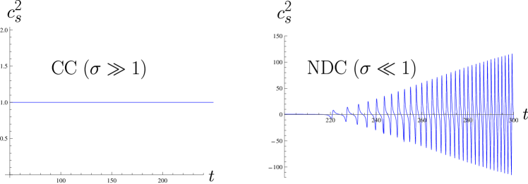
Figure 10: Sound speed squared $c_{s}^{2}$ for curvature perturbation $\zeta_{k}$ after the end of inflation: Left (CC-dominant case of CC+NDC) is nearly constant and right (NDC-dominant case of CC+NDC) oscillates increasingly after the end of inflation.

5 Perturbation analysis in the Newtonian gauge

As was shown in the previous section, the comoving gauge was not suitable for analyzing the perturbation during the reheating. This is so because the curvature perturbation $\zeta$ blows up at $\dot{\phi}=0$ on superhorizon scales. We have to re-analyze the perturbations by choosing a different gauge without problems at $\dot{\phi}=0$ [23]. To this end, we consider the scalar perturbation around the background ($\phi=\phi(t)+\varphi(t,{\bf x}))$ and the Newtonian gauge [28]. Then, the cosmological metric takes the form

$$ds^{2}_{\rm NG}=-(1+2\Psi)dt^{2}+a^{2}(t)(1-2\Phi)dx^{i}dx^{j}\delta_{ij}.$$ (5.1)

Here $\Psi$ is the Newtonian potential, while $\Phi$ is the Bardeen potential [29]. We note that $\Psi=\Phi$ in the CC, but for the Horndenski theories including the NDC, $\Psi$ is not the same with $\Phi$ [29]. It is instructive to note that the Bellini-Sawicki parametrization [30] is very useful to describe the perturbation compactly on superhorizon scales including the reheating period. It turns out that for the NDC model (2.1), the Newtonian potential $\Psi$ is related to $\Phi$ as

$$\Psi=\Phi(1+\alpha_{\rm T})\left[1-\frac{\alpha_{\rm M}-\alpha_{\rm T}}{\epsilon+\alpha_{\rm M}-\alpha_{\rm T}}\right]-\frac{\alpha_{\rm M}-\alpha_{\rm T}}{H[\epsilon+\alpha_{\rm M}-\alpha_{\rm T}]}\dot{\Phi}$$ (5.2)

with $\epsilon=-\dot{H}/H^{2}$. Considering the NDC model (2.1), one has $K=V=V_{0}\phi^{2},~{}G_{4}=M^{2}_{\rm P}/2,~{}G_{5}=-\phi/2\tilde{M}^{2}$, which determine the two parameters $\alpha_{\rm M}$ and $\alpha_{\rm T}$ as

$$\alpha_{\rm M}=-\frac{\dot{\phi}\ddot{\phi}}{H(\tilde{M}^{2}M_{\rm P}^{2}-\dot{\phi}^{2}/2)},~{}~{}~{}~{}~{}\alpha_{\rm T}=\frac{\dot{\phi}^{2}}{\tilde{M}^{2}M_{\rm P}^{2}-\dot{\phi}^{2}/2}.$$ (5.3)

Also, for the NDC model, the Hamiltonian constraint on superhorizon scales reduces to

$$\partial_{t}\left(\frac{HQ}{\dot{\phi}}\right)=0,$$ (5.4)

where $Q$ is the Mukhanov-Sasaki variable (the gauge-invariant combination)

$$Q=\varphi+\frac{\dot{\phi}}{H}\Phi.$$ (5.5)

Eq.(5.4) could be recast in terms of the Bardeen potential $\Phi$

$$\dot{\Phi}+(1+\epsilon+\alpha_{\rm M})H\Phi=CH[\epsilon+\alpha_{\rm M}-\alpha_{\rm T}],$$ (5.6)

where the constant $C$ depends on the initial conditions $\zeta_{c}$ settled during inflation when changing the Newtonian gauge to the comoving gauge.

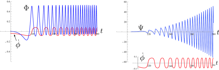
Figure 11: The behaviors of $(\Phi,\dot{\phi})$ [left] and $(\Psi,\dot{\phi})$ [right] with respect to time $t$, after the end of inflation. Both figures show that the evolutions for $\Phi$ and $\Psi$ are regular at $\dot{\phi}=0$.

In the CC+NDC model, one has $K=V=\lambda\phi^{4}/4,~{}G_{3}=-\phi/2,~{}G_{4}=M_{\rm P}^{2}/2,~{}G_{5}=-\phi/2M^{2}$ [23], where they have shown that the curvature perturbations $\zeta$ on superhorizon scales are not generally conserved but the the rescaled Mukhanov-Sasaki variable is conserved, implying a constraint equation for the Newtonian potential. This implies that the superhorizon perturbations of $\Phi$ and $\Psi$ are fine with the warning that $\Psi$ could become very large.

Coming back to the NDC model, we solve Eq.(5.6) for $\Phi$ numerically by taking into account the reheating period. Also, making use of Eq.(5.2) leads to the numerical solution for the Newtonian potential $\Psi$. Explicitly, Fig. 11 shows that after the end of inflation, the behaviors of $\Phi$ (left) and $\Psi$ (right) are regular at $\dot{\phi}=0$. Also, we observe that the Newtonian potential $\Psi$ grows very large values.

Since the subhorizon mode $\zeta_{k}$ of the curvature perturbation has suffered from the gradient instability in the comoving gauge, it is important to check whether this instability is present in the Newtonian gauge. For this purpose, we use the second-order evolution equation for the Bardeen potential mode $\Phi_{k}$ as

$$\ddot{\Phi}_{k}+\frac{\beta_{1}\beta_{2}+\beta_{3}\alpha^{2}_{\rm B}\frac{k^{2}}{a^{2}}}{\beta_{1}+\alpha^{2}_{\rm B}\frac{k^{2}}{a^{2}}}\dot{\Phi}_{k}+\frac{\beta_{1}\beta_{4}+\beta_{1}\beta_{5}\frac{k^{2}}{a^{2}}+c^{2}_{s}\alpha^{2}_{\rm B}(\frac{k^{2}}{a^{2}})^{2}}{\beta_{1}+\alpha^{2}_{\rm B}\frac{k^{2}}{a^{2}}}\Phi_{k}=0,$$ (5.7)

where the parameters $\beta_{i}(\alpha_{i},H)$ were defined in the Appendix B of Ref. [30]. Here we observe the oscillating sound speed squared $c^{2}_{s}$ (4.14) shown in Fig. 9. This equation was derived by eliminating the inflaton of $\varphi/\dot{\phi}$ which is not an observable in the Newtonian gauge. In the subhorizon regime of $k^{2}/a^{2}\gg 1$, Eq.(5.7) reduces to

$$\ddot{\Phi}_{k}+(3+\alpha_{\rm M})H\dot{\Phi}_{k}+\Big{(}\frac{\beta_{1}\beta_{5}}{\alpha^{2}_{\rm B}}+c^{2}_{s}\frac{k^{2}}{a^{2}}\Big{)}\Phi_{k}\simeq 0,$$ (5.8)

which is rewritten by introducing the Compton mass scale $k_{\rm C}$ $[k^{2}_{\rm C}c^{2}_{s}/a^{2}\equiv\beta_{1}\beta_{5}/\alpha^{2}_{\rm B}]$ [31] as

$$\ddot{\Phi}_{k}+(3+\alpha_{\rm M})H\dot{\Phi}_{k}+c^{2}_{s}\Big{(}\frac{k^{2}_{\rm C}}{a^{2}}+\frac{k^{2}}{a^{2}}\Big{)}\Phi_{k}\simeq 0.$$ (5.9)

In the case of $k^{2}/a^{2}\gg k^{2}_{\rm C}/a^{2},(3+\alpha_{\rm M})H$, the evolution equation (5.9) takes the form

$$\ddot{\Phi}_{k}+c^{2}_{s}\frac{k^{2}}{a^{2}}\Phi_{k}\simeq 0,$$ (5.10)

which leads to the gradient instability for the oscillating $c_{s}^{2}$. However, we would like to mention that in this case, the gradient instability emerges when taking the extreme quasi-static limit of the dynamics ($k\to\infty$) in the Newtonian gauge. This contrasts to the case of the comoving gauge where one could find the gradient instability easily when requiring the condition of $k^{2}/a^{2}\gg 1$ as was shown in Eq.(4.23).

6 Summary and Discussions

First of all, we have studied the difference between NDC and CC during reheating after the end of inflation. We have observed a sizable difference that the inflaton velocity $\dot{\phi}$ oscillates with damping for CC, while it oscillates without damping for NDC. We have confirmed that this difference has arisen from different time rates of their Hubble parameters ($\dot{H}$). Analytic expressions for inflaton and Hubble parameter obtained by applying the averaging method to the NDC-equations (2.6)-(2.8) [16] are not suitable for describing violent oscillations of Hubble parameter. Hence their argument of disappearing the parametric resonance is not proven for the NDC.

Now, we mention the perturbative feature for NDC generated during reheating. We have studied the curvature perturbation $\zeta$ by taking the comoving gauge ($\varphi=0$). This gauge is definitely applicable at the stage of inflation, but it may be incompatible with $\dot{\phi}=0$ during the reheating. As was shown in Eq.(4.23) in the subhorizon regime ($k^{2}/a^{2}\gg 1$), the Lagrangian instability (gradient instability) arises easily because the sound speed squared $c^{2}_{s}$ oscillates during the reheating. This presumed instability has arisen because the authors in [17] have neglected the second term of (4.22). However, this is not true for the case of the superhorizon limit ($k^{2}/a^{2}\ll 1$) as was shown in (4.24). Also, this instability never occurs even for the correction to the superhorizon mode up to $k^{2}$-order [see (4.25)]. But this case is meaningless since the second term of (4.22) is singular at $\dot{\phi}=0,\pm\phi_{c}$. Here, it is noted that the apparent singular behavior at $\dot{\phi}=\pm\phi_{c}$ disappeared at the solution level.

Importantly, it is desirable to comment on the incompatibility of the comoving gauge ($\varphi=0$) with $\dot{\phi}=0$ during the reheating in the NDC model. We remind the reader that the blow-up of $\zeta$ at $\dot{\phi}=0$ happens because the comoving gauge is not suitable for describing the oscillating period, especially for $\dot{\phi}=0$. This indicates that the curvature perturbation is not considered as a physical variable, describing a relevant perturbation during the reheating. Hence, it should not be used to draw any physical conclusion. Here the Bardeen potential $\Phi$ and Newtonian potential $\Psi$ have been employed as physical perturbations by choosing the Newtonian gauge. The superhorizon perturbations are fine with the warning that the Newtonian potential may become large. Finally, we note that the gradient instability of the Bardeen potential mode $\Phi_{k}$ appeared when taking the extremal quasi-static limit of the dynamics ($k\to\infty$) in the Newtonian gauge and thus, the NDC model would become unviable in the reheating period.

References

[1]
M. S. Turner,
Phys. Rev. D 28, 1243 (1983).
[2]
M. A. Amin, M. P. Hertzberg, D. I. Kaiser and J. Karouby,
Int. J. Mod. Phys. D 24, 1530003 (2014) doi:10.1142/S0218271815300037 [arXiv:1410.3808 [hep-ph]].
[3]
J. H. Traschen and R. H. Brandenberger,
Phys. Rev. D 42, 2491 (1990).
[4]
L. Kofman, A. D. Linde and A. A. Starobinsky,
Phys. Rev. Lett. 73, 3195 (1994) [hep-th/9405187].
[5]
L. A. Kofman,
astro-ph/9605155.
[6]
L. Kofman, A. D. Linde and A. A. Starobinsky,
Phys. Rev. D 56, 3258 (1997) [hep-ph/9704452].
[7]
J. Martin and C. Ringeval,
Phys. Rev. D 82, 023511 (2010) [arXiv:1004.5525 [astro-ph.CO]].
[8]
J. Martin, C. Ringeval and V. Vennin,
Phys. Rev. Lett. 114, no. 8, 081303 (2015) [arXiv:1410.7958 [astro-ph.CO]].
[9]
L. Amendola,
Phys. Lett. B 301, 175 (1993) [gr-qc/9302010].
[10]
S. V. Sushkov,
Phys. Rev. D 80, 103505 (2009) [arXiv:0910.0980 [gr-qc]].
[11]
C. Germani and A. Kehagias,
Phys. Rev. Lett. 105, 011302 (2010) [arXiv:1003.2635 [hep-ph]].
[12]
C. Germani and Y. Watanabe,
JCAP 1107, 031 (2011) [Addendum-ibid. 1107, A01 (2011)] [arXiv:1106.0502 [astro-ph.CO]].
[13]
C. Germani,
Rom. J. Phys. 57, 841 (2012) [arXiv:1112.1083 [astro-ph.CO]].
[14]
Y. S. Myung, T. Moon and B. H. Lee,
JCAP 1510, 007 (2015) [arXiv:1505.04027 [gr-qc]].
[15]
J. F. Donoghue, K. Dutta and A. Ross,
Phys. Rev. D 80, 023526 (2009) [astro-ph/0703455 [ASTRO-PH]].
[16]
A. Ghalee,
Phys. Lett. B 724, 198 (2013) doi:10.1016/j.physletb.2013.06.039 [arXiv:1303.0532 [astro-ph.CO]].
[17]
Y. Ema, R. Jinno, K. Mukaida and K. Nakayama,
JCAP 1510, 020 (2015)[ arXiv:1504.07119 [gr-qc]].
[18]
J. Ohashi and S. Tsujikawa,
JCAP 1210, 035 (2012) [arXiv:1207.4879 [gr-qc]].
[19]
F. Finelli and R. H. Brandenberger,
Phys. Rev. Lett. 82, 1362 (1999) [hep-ph/9809490].
[20]
K. Jedamzik, M. Lemoine and J. Martin,
JCAP 1009, 034 (2010) [arXiv:1002.3039 [astro-ph.CO]].
[21]
R. Easther, R. Flauger and J. B. Gilmore,
JCAP 1104, 027 (2011) [arXiv:1003.3011 [astro-ph.CO]].
[22]
M. T. Algan, A. Kaya and E. S. Kutluk,
JCAP 1504, no. 04, 015 (2015) [arXiv:1502.01726 [hep-th]].
[23]
C. Germani, N. Kudryashova and Y. Watanabe,
arXiv:1512.06344 [astro-ph.CO].
[24]
K. Feng and T. Qiu,
Phys. Rev. D 90, no. 12, 123508 (2014) [arXiv:1409.2949 [hep-th]].
[25]
S. Tsujikawa,
Phys. Rev. D 85, 083518 (2012) [arXiv:1201.5926 [astro-ph.CO]].
[26]
M. A. Skugoreva, S. V. Sushkov and A. V. Toporensky,
Phys. Rev. D 88, 083539 (2013) [Phys. Rev. D 88, no. 10, 109906 (2013)] [arXiv:1306.5090 [gr-qc]].
[27]
S. Weinberg,
Phys. Rev. D 72, 043514 (2005) [hep-th/0506236].
[28]
V. Mukhanov, Modern Cosmology (Amsterdam, Academic Press,2003)
p. 440.
[29]
M. Motta, I. Sawicki, I. D. Saltas, L. Amendola and M. Kunz,
Phys. Rev. D 88, no. 12, 124035 (2013)
doi:10.1103/PhysRevD.88.124035
[arXiv:1305.0008 [astro-ph.CO]].
[30]
E. Bellini and I. Sawicki,
JCAP 1407 (2014) 050
doi:10.1088/1475-7516/2014/07/050
[arXiv:1404.3713 [astro-ph.CO]].
[31]
A. De Felice and S. Tsujikawa,
Living Rev. Rel. 13, 3 (2010) doi:10.12942/lrr-2010-3 [arXiv:1002.4928 [gr-qc]].