Geodesic equations in the static and rotating dilaton black holes: Analytical solutions and applications

Abstract

In this paper, we consider the timelike and null geodesics around the static [GMGHS (Gibbons, Maeda, Garfinkle, Horowitz and Strominger), magnetically charged GMGHS, electrically charged GMGHS] and the rotating (Kerr-Sen dilaton-axion) dilaton black holes. The geodesic equations are solved in terms of Weierstrass elliptic functions. To classify the trajectories around the black holes, we use the analytical solution and effective potential techniques and then characterize the different types of the resulting orbits in terms of the conserved energy and angular momentum. Also, using the obtained results we study astrophysical applications.

I INTRODUCTION

The well-known exact solution of the vacuum Einstein equations described by Schwarzschild in 1916 K.Schwarzschild as a spherically symmetric black hole in a four dimensional spacetime. Addition of an electric charge, change the Schwarzschild solution to a charged black hole. This solution was discovered by Reissner (1916), Weyl (1917) and Nordström (1918), independently and now it is known as Reissner-Nordström metric Blaga:2014spa . Also, another solution of charged black hole in four dimensions was obtained by Gibbons and Maeda Gibbons:1987ps , independently, by Garfinkle, Horowitz and Strominger Garfinkle:1990qj using a scalar field in range of low-energy of heterotic string theory, which is called GMGHS solution Mukherjee&Majumdar . The GMGHS black hole can be explained in string or Einstein frame, which are connected to each other by conformal transformation despite of differences of the physical properties in each frames Faraoni&Gunzig&Nardone ; Casadio and Harms ; Kim&Choi&Park .

Study of motion of massive and massless particles give a set of comprehensive information about the gravitational field around a black hole. Analysis of geodesic equation of motion predict some observational phenomena such as perihelion shift, gravitational time-delay and light deflection. The first analytic solution for Schwarzschild spacetime using Weierstrassian elliptic functions and their derivatives presented by Hagihara in 1931 Y. Hagihara . The theoretical and mathematical properties of Weierstrassian elliptic functions demonstrated by Jacobi Jacobi:1841kw , Abel N.H. Abel , Riemann B. Riemann1857 ; B. Riemann1866 , Weierstrass K.T.W. Weierstrass and Baker H.F. Baker .

Analytical solutions of geodesic equations were investigated for different spacetimes such as Reissner-Nordström, Schwarzschild-(anti)de Sitter and Reissner-Nordström–(anti)–de Sitter spactime in four dimensions and in higherdimensions Chandrasekhar:1985kt ; Hackmann:2008zz ; Hackmann:2008tu . Also the motion of test particles around rotating black holes Hackmann:2010zz ; Kagramanova:2010bk and in the spacetime of a black hole which is combined by cosmic string was studied extensively Hackmann:2009rp ; Hackmann:2010ir . Recently, geodesic equations were solved analytically in the spacetime of black hole in f(R) gravity Soroushfar:2015wqa ; Soroushfar:2015dfz . Analysis of geodesics, include null, timelike Fernando:2011ki ; Olivares:2013jza , circular null and timelike geodesics Pradhan:2012id ; Blaga:2014lva , were studied in the spacetime of GMGHS black hole in the special cases.

The aim of this paper is to determine the complete set of analytic solutions of the geodesic equations in the spacetime of the static (GMGHS, magnetically charged GMGHS, electrically charged GMGHS) and rotating (Ker-Sen Dilaton-Axion) dilaton black holes. We discussed the motion of test particles and light rays in the spacetime of these black holes and present the analytic solutions of the geodesic equations in terms of the elliptic Weierstrass functions. Then we determined the type of the orbits for test particles and light rays in the vicinity of these static and rotating dilaton black holes. In the first part the static dilaton black holes is studied and In the second part the rotating dilaton black hole is analysed.

Our paper is organized as follows: In Sec. (II), we introduce the metrics and their histories for static dilaton black holes. Then we derive the geodesic equations from Lagrangian corresponding to the metric and discuss the effective potentials. We solve geodesic equations and classify the solutions of timelike and null geodesic equations. Using analytical solutions and effective potentials, we plot some possible orbits for test particles around each black hole in acceptable regions. At the end of this section, we study Astrophysical applications. In Sec. (III), we introduce the metric for a rotating dilaton black hole. Then we derive the geodesic equations and effective potential. We solve the geodesic equations analytically and plot the possible orbits. Our conclusions are drawn in Sec. (IV).

II Static Dilaton black holes

In this section, we will discuss the geodesics in the static dilaton black holes and present analytical solutions of the equations of motion.

II.1 Metrics

In this section, we review all the spacetimes which are used as static dilaton black holes. In the Einstein frame, the GMGHS action is Garfinkle:1990qj

$$S=\int d^{4}x\sqrt{-g}(R-2(\bigtriangledown\phi)^{2}-e^{-2\phi}F_{\mu\nu}F^{\mu\nu}),$$ (1)

where $\phi$ is a dilaton, $R$ is the scalar curvature, and $F_{\mu\nu}$ is the Maxwell field. The spherically symmetric static charged solutions to equations of motion of the action (1) is

$$ds_{GM}^{2}=-(1-\frac{2M}{r})dt^{2}+(1-\frac{2M}{r})^{-1}dr^{2}+r(r-\frac{Q^{2}}{M})(d\theta^{2}+\sin^{2}\theta d\varphi^{2}),$$ (2)

where $M$ and $Q$ are mass and charge, respectively. This solution was obtained by Gibbons and Maeda, and independently Garfinkle, Horowitz and Strominger with use a transformation to the Schwarzschild solution Harrison ; Blaga:2014spa .

The GMGHS action in the string frame, is

$$S=\int d^{4}x\sqrt{-g}e^{-2\phi}(R+4(\bigtriangledown\phi)^{2}-F_{\mu\nu}F^{\mu\nu}),$$ (3)

where $\phi$ is a dilaton, R is the scalar curvature, and $F_{\mu\nu}$ is the Maxwell’s field strength. String frame is related to the Einstein frame action by the conformal transformation of $g^{s}_{\mu\nu}=e^{2\phi}g^{E}_{\mu\nu}$, Gibbons:1987ps ; Garfinkle:1990qj . By going from an electrically to a magnetically charged black hole, the string metric does change with the change in sign of dilaton $\phi$, but the Einstein metric does not change. Thus, the magnetically charged GMGHS black hole metric in the string frame is given by Kim&Choi&Park ; Choi:2014wna :

$$ds_{Mag}^{2}=-\dfrac{(1-\dfrac{2M}{r})}{(1-\dfrac{Q^{2}}{Mr})}dt^{2}+\dfrac{dr^{2}}{(1-\dfrac{2M}{r})(1-\dfrac{Q^{2}}{Mr})}+r^{2}(d\theta^{2}+sin^{2}\theta d\varphi^{2}),$$ (4)

And the electrically charged GMGHS solution in the string frame is given by:

$$ds_{El}^{2}=-\dfrac{(1+\dfrac{Q^{2}-2M^{2}}{Mr})}{(1+\dfrac{Q^{2}}{Mr})^{2}}dt^{2}+\dfrac{dr^{2}}{(1+\dfrac{Q^{2}-2M^{2}}{Mr})}+r^{2}(d\theta^{2}+sin^{2}\theta d\varphi^{2}).$$ (5)

II.2 The geodesic equations

The geodesic equations can be derived by compute the Lagrangian for each metric as Chandrasekhar:1985kt

$$\mathcal{L}=\dfrac{1}{2}g_{\mu\nu}\dfrac{dx^{\mu}}{ds}\dfrac{dx^{\nu}}{ds}=\dfrac{1}{2}\epsilon,$$ (6)

where $\epsilon=0,1$ for null and timelike geodesics respectively. Thus the Lagrangian for the metric (2) is:

$$2\mathcal{L}_{GM}=-(1-\dfrac{2M}{r})\dot{t}^{2}+(1-\dfrac{2M}{r})^{-1}\dot{r}^{2}+r(r-\dfrac{Q^{2}}{M})\dot{\theta}^{2}+r(r-\dfrac{Q^{2}}{M})sin^{2}\theta\dot{\varphi}^{2},$$ (7)

for the metric (4) is:

$$2\mathcal{L}_{Mag}=-\dfrac{(1-\dfrac{2M}{r})}{(1-\dfrac{Q^{2}}{Mr})}\dot{t}^{2}+\dfrac{1}{(1-\dfrac{2M}{r})(1-\dfrac{Q^{2}}{Mr})}\dot{r}^{2}+r^{2}(\dot{\theta}^{2}+sin^{2}\theta\dot{\varphi}^{2}),$$ (8)

and for the metric (5) is:

$$2\mathcal{L}_{El}=-\dfrac{(1+\dfrac{Q^{2}-2M^{2}}{Mr})}{(1+\dfrac{Q^{2}}{Mr})^{2}}\dot{t}^{2}+\dfrac{1}{(1+\dfrac{Q^{2}-2M^{2}}{Mr})}\dot{r}^{2}+r^{2}(\dot{\theta}^{2}+sin^{2}\theta\dot{\varphi}^{2}).$$ (9)

The Killing vectors respect to the spacetime from the Euler-Lagrange for time and latitude are $\dfrac{\partial}{\partial t}$ and $\dfrac{\partial}{\partial\varphi}$. The energy $E$ and the angular momentum $L$ are the constants of motion which are given by the generalized momenta $P_{t}$ and $P_{\varphi}$

$$P_{t}=\dfrac{\partial\mathcal{L}}{\partial\dot{t}}=-E,\qquad P_{\varphi}=\dfrac{\partial\mathcal{L}}{\partial\dot{\varphi}}=L.$$ (10)

From the Euler-Lagrange equation for $t$ we get to the energy conservations

$$E_{GM}=(g_{tt})_{GM}\dfrac{dt}{ds}=-(1-\dfrac{2M}{r})\dfrac{dt}{ds},$$ (11)

$$E_{Mag}=(g_{tt})_{Mag}\dfrac{dt}{ds}=-\dfrac{(1-\dfrac{2M}{r})}{(1-\dfrac{Q^{2}}{Mr})}\dfrac{dt}{ds},$$ (12)

$$E_{El}=(g_{tt})_{El}\dfrac{dt}{ds}=-\dfrac{(1+\dfrac{Q^{2}-2M^{2}}{Mr})}{(1+\dfrac{Q^{2}}{Mr})^{2}}\dfrac{dt}{ds},$$ (13)

and for $\varphi$ we obtained the angular momentum conservations

$$L_{GM}=(g_{\varphi\varphi})_{GM}\dfrac{d\varphi}{ds}=r(r-\dfrac{Q^{2}}{M})sin^{2}\theta\dfrac{d\varphi}{ds},$$ (14)

$$L_{Mag}=(g_{\varphi\varphi})_{Mag}\dfrac{d\varphi}{ds}=r^{2}sin^{2}\theta\dfrac{d\varphi}{ds},$$ (15)

$$L_{El}=(g_{\varphi\varphi})_{El}\dfrac{d\varphi}{ds}=r^{2}sin^{2}\theta\dfrac{d\varphi}{ds}.$$ (16)

We consider the motion is took place in a equatorial plane because of the existence of spherically symmetry and choose $\theta=\frac{\pi}{2}$ and $\dot{\theta}=0$ as the initial conditions. Therefore with substitute $\dot{t}$ and $\dot{\varphi}$ from Eqs.(11)-(16), in Eqs.(7)-(9), we get

$$(\dfrac{dr}{ds})_{GM}^{2}=E_{GM}^{2}-(1-\dfrac{2M}{r})(\dfrac{L_{GM}^{2}}{r(r-\frac{Q^{2}}{M})}+\epsilon),$$ (17)

$$(\dfrac{dr}{ds})_{Mag}^{2}=(1-\dfrac{Q^{2}}{Mr})^{2}E_{Mag}^{2}-(1-\dfrac{2M}{r})(1-\dfrac{Q^{2}}{Mr})(\dfrac{L_{Mg}^{2}}{r^{2}}+\epsilon),$$ (18)

$$(\dfrac{dr}{ds})_{El}^{2}=(1+\dfrac{Q^{2}}{Mr})^{2}E_{El}^{2}-(1+\dfrac{Q^{2}-2M^{2}}{Mr})(\dfrac{L_{El}^{2}}{r^{2}}+\epsilon).$$ (19)

We obtain the corresponding equation for $r$ as a function of $\varphi$ and as a function of $t$, with energy and angular momentum conservation

$$(\dfrac{dr}{d\varphi})^{2}_{GM}=(\dfrac{E^{2}}{L^{2}}-\dfrac{\epsilon}{L^{2}})r^{4}+(\dfrac{-2E^{2}Q^{2}}{ML^{2}}+\dfrac{2\epsilon Q^{2}}{ML^{2}}+\dfrac{2M\epsilon}{L^{2}})r^{3}+(\dfrac{E^{2}Q^{4}}{M^{2}L^{2}}-$$

$$-\dfrac{\epsilon Q^{4}}{M^{2}L^{2}}-\dfrac{4\epsilon Q^{2}}{L^{2}}-1)r^{2}+(\dfrac{2\epsilon Q^{4}}{ML^{2}}+\dfrac{Q^{2}}{M}+2M)r-2Q^{2}=R_{GM}(r),$$ (20)

$$(\dfrac{dr}{d\varphi})^{2}_{Mag}=(\dfrac{E^{2}}{L^{2}}-\dfrac{\epsilon}{L^{2}})r^{4}+(\dfrac{-2E^{2}Q^{2}}{ML^{2}}+\dfrac{\epsilon Q^{2}}{ML^{2}}+\dfrac{2M\epsilon}{L^{2}})r^{3}+$$

$$+(\dfrac{E^{2}Q^{4}}{M^{2}L^{2}}-\dfrac{2\epsilon Q^{2}}{L^{2}}-1)r^{2}+(\dfrac{Q^{2}}{M}+2M)r-2Q^{2}=R_{Mag}(r),$$ (21)

$$(\dfrac{dr}{d\varphi})^{2}_{El}=(\dfrac{E^{2}}{L^{2}}-\dfrac{\epsilon}{L^{2}})r^{4}+(\dfrac{2E^{2}Q^{2}}{ML^{2}}-\dfrac{\epsilon Q^{2}}{ML^{2}}+\dfrac{2M\epsilon}{L^{2}})r^{3}+$$

$$+(\dfrac{E^{2}Q^{4}}{M^{2}L^{2}}-1)r^{2}+(-\dfrac{Q^{2}}{M}+2M)r=R_{El}(r),$$ (22)

and

$$(\dfrac{dr}{dt})_{GM}^{2}=\frac{1}{E^{2}}(1-\frac{2M}{r})^{2}[E^{2}-(1-\frac{2M}{r})(\dfrac{L^{2}}{r(r-\frac{Q^{2}}{M})}+\epsilon)],$$ (23)

$$(\dfrac{dr}{dt})_{Mag}^{2}=\frac{1}{E^{2}}\dfrac{(1-\frac{2M}{r})^{2}}{(1-\dfrac{Q^{2}}{Mr})^{2}}[(1-\dfrac{Q^{2}}{Mr})^{2}E^{2}-(1-\frac{2M}{r})(1-\frac{Q^{2}}{Mr})(\frac{L^{2}}{r^{2}}+\epsilon)],$$ (24)

$$(\dfrac{dr}{dt})_{El}^{2}=\frac{1}{E^{2}}\dfrac{(1+\dfrac{Q^{2}-2M^{2}}{Mr})^{2}}{(1+\frac{Q^{2}}{Mr})^{2}}[(1+\frac{Q^{2}}{Mr})^{2}E^{2}-(1+\dfrac{Q^{2}-2M^{2}}{Mr})(\frac{L^{2}}{r^{2}}+\epsilon)].$$ (25)

Eqs.(17)-(25) gives a complete definition of the dynamics. In these set of equations, the values of $L$ and $E^{2}$ in the right hand side refer to indices of the left hand side of them, that we ignore indices for $L$ and $E^{2}$ for simplicity. We get the effective potential by comparing Eqs.(17)-(19) with $\dot{r}^{2}+V_{eff}=E^{2}$,

$$(V_{eff})_{GM}=(1-\dfrac{2M}{r})(\dfrac{L^{2}}{r(r-\frac{Q^{2}}{M})}+\epsilon),$$ (26)

$$(V_{eff})_{Mag}=\dfrac{(1-\dfrac{2M}{r})(\dfrac{L^{2}}{r^{2}}+\epsilon)}{(1-\dfrac{Q^{2}}{Mr})},$$ (27)

$$(V_{eff})_{El}=-\dfrac{(1+\dfrac{Q^{2}-2M^{2}}{Mr})(\dfrac{L^{2}}{r^{2}}+\epsilon)}{(1+\dfrac{Q^{2}}{Mr})^{2}},$$ (28)

which depends on radial coordinate $r$, charge $Q$ and mass $M$ of the black hole, the type of the geodesics $\epsilon$ and the angular momentum $L$ of the particles. In these set of equations, again the value of $L$ in the right hand side refer to indices of the left hand side of them, that we ignore indices for $L$ and $E^{2}$ for simplicity.

We introduce dimensionless quantities for rescale the parameters

$$\tilde{r}=\frac{r}{M},\qquad\tilde{Q}=\frac{Q}{M},\qquad\tilde{L}=\dfrac{M^{2}}{L^{2}},$$ (29)

and rewrite Eqs.(II.2)-(II.2) as

$$(\dfrac{d\tilde{r}}{d\varphi})^{2}_{GM}=(E^{2}-\epsilon)\tilde{L}\tilde{r}^{4}+(2\tilde{Q}^{2}\epsilon+2\epsilon-2E^{2}\tilde{Q}^{2})\tilde{L}\tilde{r}^{3}+(E^{2}\tilde{Q}^{4}\tilde{L}$$

$$-\epsilon\tilde{Q}^{4}\tilde{L}-4\tilde{Q}^{2}\epsilon\tilde{L}-1)\tilde{r}^{2}+(2\epsilon\tilde{Q}^{4}\tilde{L}+\tilde{Q}^{2}+2)\tilde{r}-2\tilde{Q}^{2}=R_{GM}(\tilde{r}),$$ (30)

$$(\dfrac{d\tilde{r}}{d\varphi})^{2}_{Mag}=(E^{2}-\epsilon)\tilde{L}\tilde{r}^{4}+(\tilde{Q}^{2}\epsilon-2\tilde{Q}^{2}E^{2}+2\epsilon)\tilde{L}\tilde{r}^{3}+$$

$$(\tilde{Q}^{4}E^{2}\tilde{L}-2\tilde{Q}^{2}\epsilon\tilde{L}-1)\tilde{r}^{2}+(\tilde{Q}^{2}+2)\tilde{r}-2\tilde{Q}^{2}=R_{Mag}(\tilde{r}),$$ (31)

$$(\dfrac{d\tilde{r}}{d\varphi})^{2}_{El}=(E^{2}-\epsilon)\tilde{L}\tilde{r}^{4}+(2\tilde{Q}^{2}E^{2}-\tilde{Q}^{2}\epsilon+2\epsilon)\tilde{L}\tilde{r}^{3}$$

$$+(\tilde{Q}^{4}E^{2}\tilde{L}-1)\tilde{r}^{2}+(-\tilde{Q}^{2}+2)\tilde{r}=R_{El}(\tilde{r}).$$ (32)

Also, in these set of equations, the values of $\tilde{L}$ and $E^{2}$ in the right hand side refer to indices of the left hand side of them, that we ignore indices for $\tilde{L}$ and $E^{2}$ for simplicity.

II.3 Analytical solution of geodesic equations

In this section, we present the solution of the equations of motion analytically. In the Eqs.(II.2)-(II.2) for the test particle ($\epsilon=1$) and light ray ($\epsilon=0$), we have polynomials of degree four in the form $R(\tilde{r})=\sum_{i=0}^{4}a_{i}\tilde{r}^{i}$, with only simple zeros, which for solving them in this way, we can apply up to two substitutions. The first substitution is $\tilde{r}=\frac{1}{z}+\tilde{r}_{R}$ , where $\tilde{r}_{R}$ is a zero of $R$, transforms the problem to

$$(\dfrac{dz}{d\varphi})^{2}=R_{3}(z)=\sum_{j=1}^{3}b_{j}z^{j},\qquad z(\varphi_{0})=z_{0},$$ (33)

with a polynomial $R_{3}$ of degree 3. Where

$$b_{j}=\dfrac{1}{(4-j)!}\dfrac{d^{(4-j)}R}{d\tilde{r}^{(4-j)}}(\tilde{r}_{R}),$$ (34)

in which $b_{j},~{}(j=1,2,3)$ is an arbitrary constant for each metric which is related to the parameter of the relevant metric. A second substitution $z=\frac{1}{b_{3}}(4y-\frac{b_{2}}{3})$, changes $R_{3}(z)$, into the Weierstrass form

$$(\dfrac{dy}{d\varphi})^{2}=4y^{3}-g_{2}y-g_{3},$$ (35)

where

$$g_{2}=\frac{1}{16}(\frac{4}{3}b_{2}^{2}-4b_{1}b_{3}),\qquad g_{3}=\frac{1}{16}(\frac{1}{3}b_{1}b_{2}b_{3}-\frac{2}{27}b_{2}^{3}-b_{0}b_{3}^{2}),$$ (36)

are the Weierstrass invariants. The differential equation(35) is of elliptic type and we used the Weierstrass $\wp$ function to solve it Hackmann:2008zz ; Soroushfar:2015wqa

$$y(\varphi)=\wp(\varphi-\varphi_{in};g_{2},g_{3}),$$ (37)

where $\varphi_{in}=\varphi_{0}+\int_{y_{0}}^{\infty}\dfrac{dy}{\sqrt{4y^{3}-g_{2}y-g_{3}}}$ with $\varphi_{0}=\frac{1}{4}(\dfrac{b_{3}}{\tilde{r_{0}}-\tilde{r_{R}}}+\dfrac{b_{2}}{3})$ depends only on the initial values $\varphi_{0}$ and $\tilde{r}_{0}$. Therefore, the solution of Eqs.(II.2)-(II.2) takes the form

$$\tilde{r}(\varphi)=\dfrac{b_{3}}{4\wp(\varphi-\varphi_{in};g_{2},g_{3})-\dfrac{b_{2}}{3}}+\tilde{r}_{R}.$$ (38)

This is the analytic solution of the equation of motion of a test particle and light ray in a GMGHS, magnetically charged GMGHS and electrically charged GMGHS spacetimes. This solution is valid in all regions of this spacetimes.

II.4 Orbits

In a special spacetime with electric charge, the shape of an orbit depends on three paremeters, in which the angular momentum, $L$ and the energy, $E$ are the specifications of test particle or light ray and the electric charge, $Q$ comes from the related spacetime (the mass can be absorbed through a rescaling of the radial coordinate). The polynomial $R(r)$ defined in Eqs.(II.2)-(II.2) are included all these quantities. Since $r$ should be real and positive, the physically admissible regions are given by those $r$ for which $E^{2}\geq V_{eff}$ which is presented on the left hand side of Eqs.(17)-(19). Therefore, the form of the resulting orbits are characterized uniquely by the number of positive real zeros of $R$.

In the following, we introduce different types of orbit. Let $\tilde{r}_{+}$ be the outer event horizon and $\tilde{r}_{-}$ be the inner horizon.

1. Escape orbit (EO) with range $\tilde{r}\in[r_{1},\infty)$ with $r_{1}>\tilde{r}_{+}$, or with range $\tilde{r}\in(-\infty,r_{1}]$ with $r_{1}<0$.

2. Two-world escape orbit (TEO) with range $[r_{1},\infty)$ where $0<r_{1}<r_{-}$.

3. Bound orbit (BO) with range $\tilde{r}\in[r_{1},r_{2}]$ with

   1. $r_{1},r_{2}>r_{+}$, or

   2. $0<r_{1},r_{2}<r_{-}$.

4. Many-world bound orbit (MBO) with range $\tilde{r}\in[r_{1},r_{2}]$ where $0<r_{1}\leq r_{-}$ and $r_{2}\geq r_{+}$.

5. Terminating orbit (TO) with ranges either $\tilde{r}\in[0,\infty)$ or $\tilde{r}\in[0,r_{1}]$ with

   1. $r_{1}\geq\tilde{r}_{+}$, or

   2. $0<r_{1}<\tilde{r}_{-}$.

Other types of orbits are exceptional and treated separately. They are connected with the appearance of multiple zeros in $R(r)$ or with parameter values which reduce the degree of $R(r)$. In both cases the differential Eqs.(II.2)-(II.2) have much simplified structure. These orbits are radial geodesics with $L=0$, circular orbits with constant $r$ and orbits asymptotically approaching circular orbits.

Defining the borders of $R(r)\geq 0$ or, equivalently, $E^{2}\geq V_{eff}$ is done by the four regular types of geodesic motion correspond to various arrangements of the real and positive zeros of $R(r)$. If $R(r)$ has no real and positive zeros, a terminating orbit is possible if $R(r)>0$ for all $r>0$, but else no geodesic motion is allowed. If $R(r)$ has at least one real and positive zero then an escape orbit is possible, or a terminating orbit if $R(r)>0$ for $0<r<r_{1}$, where, $r_{1}$ is the smallest positive zero. If $R(r)$ has at least two real zeros, $r_{1}<r_{2}$ with $R(r)>0$ for $r_{1}<r<r_{2}$ a bound orbit is permitted. If $R(r)$ is such that, multiple types of orbits are possible, then the actual orbit depends on the initial position of the test particle or light ray.

In the following, we will analyse possible types of orbits. The major point in this analysis is that Eqs.(II.2)-(II.2) implies $R(\tilde{r})\geq 0$, as a necessary condition for the existence of a geodesic. Thus, the zeros of $R(\tilde{r})$, are extremal values of $\tilde{r}(\varphi)$ and determine (together with the sign of $R(\tilde{r})$ between two zeros) the type of geodesic. The polynomial $R(\tilde{r})$ is in our metrics of degree 4 and, therefore, has 4 (complex) zeros of which the positive real zeros are of interest for the type of orbit.

For a given set of parameters $\epsilon,E^{2},\tilde{Q}$, and $\tilde{L}$ the polynomial $R(\tilde{r})$ has a certain number of positive real zeros. If $E^{2}$ and $\tilde{L}$ are varied, this number can change only if two zeros of $R(\tilde{r})$ merge to one. Solving $R(\tilde{r})=0$ , $\dfrac{dR(\tilde{r})}{d\tilde{r}}=0$ for $E^{2}$ and $\tilde{L}$, for $\epsilon=1$ yields

$$E_{GM}^{2}=\dfrac{\tilde{Q}^{2}\tilde{r}^{2}-4\tilde{Q}^{2}\tilde{r}-2\tilde{r}^{3}+4\tilde{Q}^{2}+8\tilde{r}^{2}-8\tilde{r}}{(\tilde{Q}^{2}\tilde{r}-4\tilde{Q}^{2}-2\tilde{r}^{2}+6\tilde{r})\tilde{r}},\qquad\tilde{L}_{GM}=-\frac{1}{2}\dfrac{\tilde{Q}^{2}\tilde{r}-4\tilde{Q}^{2}-2\tilde{r}^{2}+6\tilde{r}}{\tilde{r}(\tilde{Q}^{4}-2\tilde{Q}^{2}\tilde{r}+\tilde{r}^{2})},$$ (39)

$$E_{Mag}^{2}=-\dfrac{2(\tilde{r}^{2}-4\tilde{r}+4)}{\tilde{Q}^{2}\tilde{r}-4\tilde{Q}^{2}-2\tilde{r}^{2}+6\tilde{r}},\qquad\tilde{L}_{Mag}=\dfrac{\tilde{Q}^{2}\tilde{r}-4\tilde{Q}^{2}-2\tilde{r}^{2}+6\tilde{r}}{\tilde{r}^{3}(\tilde{Q}^{2}-2)},$$ (40)

$$E_{El}^{2}=\dfrac{2(\tilde{Q}^{4}+2\tilde{Q}^{2}\tilde{r}-4\tilde{Q}^{2}+\tilde{r}^{2}-4\tilde{r}+4)\tilde{r}}{(\tilde{Q}^{2}+\tilde{r})(\tilde{Q}^{4}+3\tilde{Q}^{2}\tilde{r}-2\tilde{Q}^{2}+2\tilde{r}^{2}-6\tilde{r})},\qquad\tilde{L}_{El}=\dfrac{\tilde{Q}^{4}+3\tilde{Q}^{2}\tilde{r}-2\tilde{Q}^{2}+2\tilde{r}^{2}-6\tilde{r}}{\tilde{r}^{2}(\tilde{Q}^{4}+\tilde{Q}^{2}\tilde{r}-2\tilde{Q}^{2}+2\tilde{r})}.$$ (41)

In Fig.1(a), the result of this analysis is shown for test particles ($\epsilon=1$). For light rays $(\epsilon=0)$, the analysis is the same as in the $(\epsilon=1)$ case and the result of this analysis is shown in Fig.1(b).

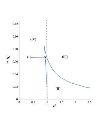
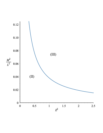
Figure 1: Regions of different types of geodesic motion for test particles, in GMGHS, magnetically charged and electrically charged GMGHS spacetimes. $\tilde{Q}=0.25$, $\epsilon=1$ and $\epsilon=0$, for (a) and (b) respectively. The numbers of positive real zeros in these regions are: I=4, II=3, III=1 and IV=2, for GMGHS, magnetically charged GMGHS spacetimes and I=3, II=2, III=0 and IV=1, for electrically charged GMGHS spacetime.

Four different regions can be identified in Fig.1, for timelike geodesic but for null geodesic, in Fig.1(b), we have only two regions. It should be noted that, for electrically charged GMGHS metric, the number of zeros is one more less than zeros of GMGHS and magnetically charged GMGHS metrics in each region. Summary of possible orbit types can be found in Tabels 1 and 2.

region	pos.zeros	range of $\tilde{r}$	orbit
I	4	(-3,-0.2)(2.2,0.2)[linewidth=0.5pt]-¿(-2.5,0)(1.75,0) [linewidth=0.5pt](-2.5,-0.2)(-2.5,0.2) [linewidth=0.5pt,doubleline=true](-2.25,-0.2)(-2.25,0.2) [linewidth=0.5pt,doubleline=true](-1.25,-0.2)(-1.25,0.2) [linewidth=1.2pt]*-*(-2.25,0)(-0.75,0) [linewidth=1.2pt]*-*(0.25,0)(1.25,0)	MBO, BO
II	3	(-3,-0.2)(2.2,0.2)[linewidth=0.5pt]-¿(-2.5,0)(1.75,0) [linewidth=0.5pt](-2.5,-0.2)(-2.5,0.2) [linewidth=0.5pt,doubleline=true](-2.25,-0.2)(-2.25,0.2) [linewidth=0.5pt,doubleline=true](-1.25,-0.2)(-1.25,0.2) [linewidth=1.2pt]*-*(-2.25,0)(-0.75,0) [linewidth=1.2pt]*-(0.25,0)(1.75,0)	EO و MBO
III	1	(-3,-0.2)(2.2,0.2)[linewidth=0.5pt]-¿(-2.5,0)(1.75,0) [linewidth=0.5pt](-2.5,-0.2)(-2.5,0.2) [linewidth=0.5pt,doubleline=true](-2.25,-0.2)(-2.25,0.2) [linewidth=0.5pt,doubleline=true](-1.25,-0.2)(-1.25,0.2) [linewidth=1.2pt]*-(-2.25,0)(1.75,0)	TEO
IV	2	(-3,-0.2)(2.2,0.2)[linewidth=0.5pt]-¿(-2.5,0)(1.75,0) [linewidth=0.5pt](-2.5,-0.2)(-2.5,0.2) [linewidth=0.5pt,doubleline=true](-2.25,-0.2)(-2.25,0.2) [linewidth=0.5pt,doubleline=true](-1.25,-0.2)(-1.25,0.2) [linewidth=1.2pt]*-*(-2.25,0)(-0.75,0)	MBO

Table 1: Types of orbits of GMGHS and magnetically GMGHS black holes. The range of the orbits is represented by thick lines. The dots show the turning points of the orbits. The positions of the two horizons are marked by a vertical double line. The single vertical line indicates $\tilde{r}=0$.

region	pos.zeros	range of $\tilde{r}$	orbit
I	3	(-3,-0.2)(2.2,0.2)[linewidth=0.5pt]-¿(-2.5,0)(1.75,0) [linewidth=0.5pt](-2.5,-0.2)(-2.5,0.2) [linewidth=0.5pt,doubleline=true](-1.25,-0.2)(-1.25,0.2) [linewidth=1.2pt]-*(-2.5,0)(-0.75,0) [linewidth=1.2pt]*-*(0.25,0)(1.25,0)	TO, BO
II	2	(-3,-0.2)(2.2,0.2)[linewidth=0.5pt]-¿(-2.5,0)(1.75,0) [linewidth=0.5pt](-2.5,-0.2)(-2.5,0.2) [linewidth=0.5pt,doubleline=true](-1.25,-0.2)(-1.25,0.2) [linewidth=1.2pt]-*(-2.5,0)(-0.75,0) [linewidth=1.2pt]*-(0.25,0)(1.75,0)	TO, EO
III	0	(-3,-0.2)(2.2,0.2)[linewidth=0.5pt]-¿(-2.5,0)(1.75,0) [linewidth=0.5pt](-2.5,-0.2)(-2.5,0.2) [linewidth=0.5pt,doubleline=true](-1.25,-0.2)(-1.25,0.2) [linewidth=1.2pt]-(-2.5,0)(1.75,0)	TO
IV	1	(-3,-0.2)(2.2,0.2)[linewidth=0.5pt]-¿(-2.5,0)(1.75,0) [linewidth=0.5pt](-2.5,-0.2)(-2.5,0.2) [linewidth=0.5pt,doubleline=true](-1.25,-0.2)(-1.25,0.2) [linewidth=1.2pt]-*(-2.5,0)(-0.75,0)	TO

Table 2: Types of orbits of electrically GMGHS black hole. The range of the orbits is represented by thick lines. The dots show the turning points of the orbits. The positions of the one horizon is marked by a vertical double line. The single vertical line indicates $\tilde{r}=0$.

In the following, we give a list of existence regions (for Fig. 1 and tables 1 and 2). For each region, examples of effective potentials and possible orbit types are demonstrated in Figs. 2–4.

1. In region I, for GMGHS and magnetically charged GMGHS black holes, $R(\tilde{r})$ has 4 positive real zeros $r_{1}<r_{2}<r_{3}<r_{4}$ with $R(\tilde{r})\geq 0$ for $r_{1}\leq\tilde{r}\leq r_{2}$ and $r_{3}\leq\tilde{r}\leq r_{4}$. Therefore the possible orbit types are bound and Mani-world bound orbits, respectively [see Figs. 2 (a), 3 (a), and 3 (d)]. But in this region for electrically charged GMGHS black hole, $R(\tilde{r})$ has 3 positive real zeros $r_{1}<r_{2}<r_{3}$ with $R(\tilde{r})\geq 0$ for $0\leq\tilde{r}\leq r_{1}$ and $r_{2}\leq\tilde{r}\leq r_{3}$. Therefore the possible orbit types are terminating and bound orbits, respectively [see Figs. 2 (c), 4 (a), and 4 (b)].

2. In region II, for GMGHS and magnetically charged GMGHS black holes, $R(\tilde{r})$ has 3 positive real zeros $r_{1}<r_{2}<r_{3}$ with $R(\tilde{r})\geq 0$ for $r_{1}\leq\tilde{r}\leq r_{2}$ and $r_{3}\leq\tilde{r}$. Therefore the possible orbit types are Mani-world bound and escape orbits, respectively [see Figs. 2 (b), 3 (d), and 3 (c)]. But in this region for electrically charged GMGHS black hole, $R(\tilde{r})$ has 2 positive real zeros $r_{1}<r_{2}$ with $R(\tilde{r})>0$ for $0\leq\tilde{r}\leq r_{1}$ and $r_{2}\leq\tilde{r}$. Therefore the possible orbit types are terminating and escape orbits, respectively [see Figs. 2 (d), 4 (a) and 4 (c)].

3. In region III, for GMGHS and magnetically charged GMGHS black holes, $R(\tilde{r})$ has 1 positive real zero $r_{1}$ with $R(\tilde{r})\geq 0$ for $r_{1}\leq\tilde{r}$. Therefore the possible orbit type is the two-world escape orbit [see Figs. 2 (b) and 3 (b)]. But in this region for electrically charged GMGHS black hole, $R(\tilde{r})$ has 0 positive real zeros and $R(\tilde{r})\geq 0$ for $0\leq\tilde{r}$. Therefore the possible orbit type is terminating orbit [see Figs. 2 (d) and 4 (a)].

4. In region IV, for GMGHS and magnetically charged GMGHS black holes, $R(\tilde{r})$ has 2 positive real zeros $r_{1}$,$r_{2}$ with $R(\tilde{r})\geq 0$ for $r_{1}\leq\tilde{r}\leq r_{2}$. Therefore the possible orbit type is Mani-world bound orbit [see Figs. 2 (b) and 3 (d)]. But in this region for electrically charged GMGHS black hole, for electrically charged GMGHS black hole, $R(\tilde{r})$ has 1 positive real zero $r_{1}$ with $R(\tilde{r})\geq 0$ for positive $r$. Therefore the possible orbit type is terminating orbit [see Figs. 2 (d) and 4 (a)].

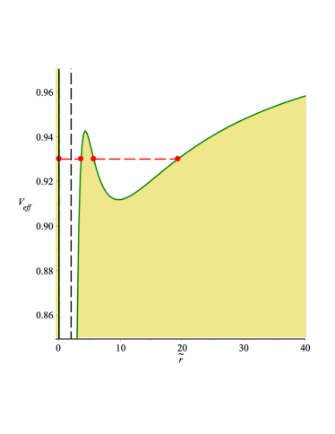
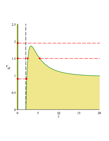
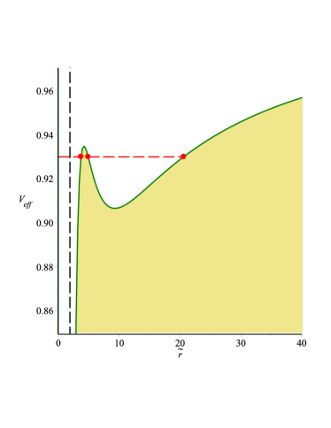
Figure 2: Plots of the effective potential together with examples of energies for the different orbit types. (a), (b) correspond to Table 1 and (c), (d) correspond to Table 2. The green curves represent the effective potential. The red dashed lines correspond to energies. The red dots mark the zeros of the polynomial $R$, which are the turning points of the orbits. In the khaki area no motion is possible since $\tilde{R}<0$. The vertical black dashed lines show the position of the horizons. $\epsilon=1$, $\tilde{Q}=0.25$, and $\tilde{L}=0.072$ for (a), (c) and $\tilde{L}=0.025$ for (b), (d).

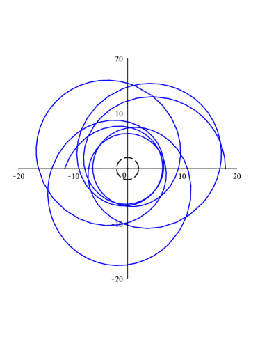
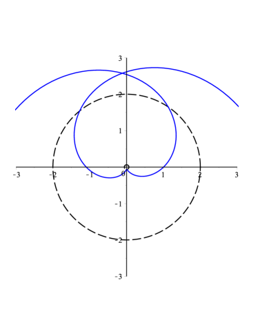
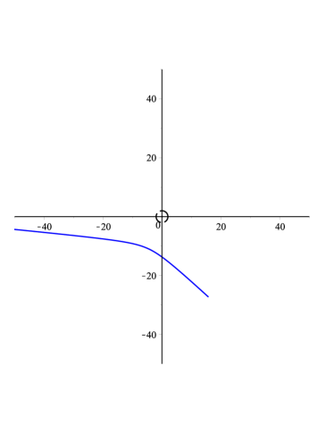
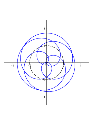
Figure 3: Four examples of possible orbits in the spacetime of GMGHS and magnetically charged GMGHS black holes. A bound orbit (a), a two-world escape orbit (c), an escape orbit and a Mani-world bound orbit (d), with parameters $\epsilon=1$, $\tilde{Q}=0.25$ and $L=0.072$, $E=\sqrt{0.93}$ for (a), (d) and $L=0.025$, $E=\sqrt{1.94}$ for (b) and $L=0.025$, $E=\sqrt{1.5}$ for (c). The blue lines show the path of the orbits and the circles represent the inner and outer horizons.

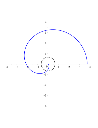
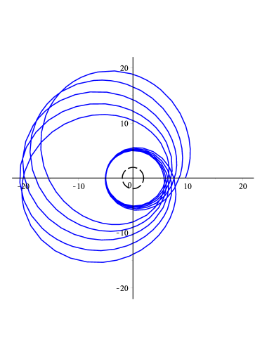
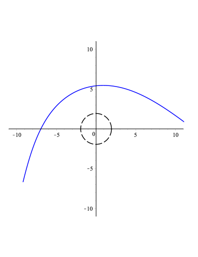
Figure 4: Three examples of possible orbits in the spacetime of a electrically charged GMGHS black hole. A bound orbit (a), a terminating orbit (b) and an escape orbit (c), with parameters $\epsilon=1$, $\tilde{Q}=0.25$ and $L=0.072$, $E=\sqrt{0.93}$ for (a), $L=0.025$, $E=\sqrt{1.94}$ for (b) and $L=0.025$, $E=\sqrt{1.5}$ for (c). The blue lines show the path of the orbits and the circle represents the event horizon.

II.5 Astrophysical applications

II.5.1 Deflection of light

The deflection of light in a Schwarzschild de Sitter spacetime was discussed by Rindler and Ishak Rindler:2007zz . Though the equation of motion is the same as in Schwarzschild spacetime for identical periapsis $r_{p}$, they showed that the measuring process for angles reintroduces the effect of the cosmological constant. Also, this method was applied in a more general solution of Weyl conformal gravity in Refs. Bhattacharya:2009rv , Bhattacharya:2010xh .

According to their scheme, they used the invariant formula for the cosine of the angle between two coordinate directions $d$ and $\delta$, as

$$\cos(\psi)=\dfrac{g_{ij}d^{i}\delta^{j}}{(g_{ij}d^{i}d^{j})^{\frac{1}{2}}(g_{ij}\delta^{i}\delta^{j})^{\frac{1}{2}}}.$$ (42)

For our purpose the relevant $g_{ij}$ is

$$(g_{rr})_{GM}=(1-\frac{2M}{r})^{-1},\qquad(g_{\varphi\varphi})_{GM}=r(r-\frac{Q^{2}}{M}),$$

$$(g_{rr})_{Mag}=\Big{(}(1-\dfrac{2M}{r})(1-\dfrac{Q^{2}}{Mr})\Big{)}^{-1},\qquad(g_{\varphi\varphi})_{Mag}=r^{2},$$

$$(g_{rr})_{El}=\Big{(}1+\dfrac{Q^{2}-2M^{2}}{Mr}\Big{)}^{-1},\qquad(g_{\varphi\varphi})_{Mag}=r^{2}.$$ (43)

Then, if we call the direction of the orbit $d$ and that of the coordinate line $\varphi=const\delta$ , we have

$$d =(dr,d\varphi)=(\dfrac{dr}{d\varphi},1)d\varphi,\qquad(d\varphi<0),$$ (44)

$$\delta =(\delta r,0)=(1,0)\delta r.$$ (45)

Substituted into (42), these values yield

$$\cos(\psi)=\dfrac{(\dfrac{dr}{d\varphi})}{\sqrt{(\dfrac{dr}{d\varphi})^{2}+(\dfrac{g_{\varphi\varphi}}{g_{rr}})}},$$ (46)

or more conveniently, the exact angle between the radial direction and the spatial direction of the light ray is now given by

$$\tan(\psi)=\dfrac{\sqrt{\dfrac{g_{\varphi\varphi}}{g_{rr}}}}{\mid\dfrac{dr}{d\varphi}\mid}.$$ (47)

Thus, according to Eq.(47), we have

$$\tan(\psi)_{GM}=\sqrt{\dfrac{\Big{(}1-\dfrac{2M}{r(\varphi)}\Big{)}r_{p}\Big{(}r_{p}-\dfrac{Q^{2}}{M}\Big{)}}{\Big{(}1-\dfrac{2M}{r_{p}}\Big{)}r(\varphi)\Big{(}r(\varphi)-\dfrac{Q^{2}}{M}\Big{)}-\Big{(}1-\dfrac{2M}{r(\varphi)}\Big{)}r_{p}\Big{(}r_{p}-\dfrac{Q^{2}}{M}\Big{)}}},$$ (48)

for GMGHS spacetime,

$$\tan(\psi)_{Mag}=\sqrt{\dfrac{r_{p}^{4}\Big{(}1-\dfrac{Q^{2}}{Mr_{p}}\Big{)}^{2}}{\dfrac{r_{p}^{2}\Big{(}1-\dfrac{2M}{r_{p}}\Big{)}\Big{(}1-\dfrac{Q^{2}}{Mr_{p}}\Big{)}r(\varphi)^{4}\Big{(}1-\dfrac{Q^{2}}{Mr(\varphi)}\Big{)}^{2}}{\Big{(}r(\varphi)^{2}(1-\dfrac{2M}{r(\varphi)})(1-\dfrac{Q^{2}}{Mr(\varphi)})\Big{)}}-r_{p}^{4}\Big{(}1-\dfrac{Q^{2}}{Mr_{p}}\Big{)}^{2}}},$$ (49)

for magnetically charged GMGHS spacetime, and

$$\tan(\psi)_{El}=\sqrt{\dfrac{r(\varphi)^{2}\Big{(}1+\dfrac{Q^{2}-2M^{2}}{Mr(\varphi)}\Big{)}r_{p}^{2}\Big{(}r_{p}+\dfrac{Q^{2}}{M}\Big{)}^{2}}{r_{p}^{2}\Big{(}1+\dfrac{Q^{2}-2M^{2}}{Mr_{p}}\Big{)}-r(\varphi)^{2}\Big{(}1+\dfrac{Q^{2}-2M^{2}}{Mr(\varphi)}\Big{)}r_{p}^{2}\Big{(}r_{p}+\dfrac{Q^{2}}{M}\Big{)}^{2}}},$$ (50)

for electrically charged GMGHS spacetime.

where, $r(\varphi)$ is the solutions of Eqs.(II.2)-(II.2) which solved in Eq.(38) for $\epsilon=0$. These now are valid for all light rays, not only for those rays showing a small deflection as discussed in Refs. Rindler:2007zz ; Bhattacharya:2009rv ; Bhattacharya:2010xh .

II.5.2 Periastron advance of bound timelike orbits

In the case that $R(r)$ (Eqs.(II.2)-(II.2)) has at least two positive zeros, we may have a bound orbit for some initial values. The periastron advance $\Delta_{peri}$ for such a bound orbit is given by the difference of the $2\pi$-periodicity of the angle $\varphi$ and the periodicity of the solution $r(\varphi)$  Kraniotis:2003ig ; Kraniotis:2004cz ,

$$\Delta^{Dilaton}_{peri}=2(\omega-\pi).$$ (51)

The equations of motion for the static dilaton (GMGHS, magnetically GMGHS and electrically GMGHS) black hole and the rotating dilaton (The Ker-Sen Dilaton-Axion) black hole, which is described in sec.III.1, are polynomials of degree four and can be solved in terms of Weierstrass elliptic functions similarly. So, for example, we consider the electrically GMGHS black hole and calculate physical data i.e. the aphel $r_{A}$ , the perihel $r_{p}$, and the perihelion advance. For the calculation of the perihelion precession and the orbital characteristics of Mercury we use the following values for the physical constants:

$$c=2.99792458\times 10^{10}\rm{cm}s^{-1},\qquad\alpha_{S}=\dfrac{2GM_{\bigodot}}{c^{2}}=2.95325008\times 10^{5}\rm{cm}.$$ (52)

As free parameters we may use $\mathcal{L}$ and $E$ given in Refs. Hackmann:2008zz ; Kraniotis:2003ig ,

$$\mathcal{L}=1.1849627128268641\times 10^{-28}\rm{cm}^{-2}s^{2},\qquad E=0.029979245417779875\times 10^{12}\rm{cm}s^{-1}.$$ (53)

The two half-periods $\omega$ and $\omega^{\prime}$ are given by the following Abelian integrals

$$\omega=\int_{e_{1}}^{\infty}\frac{dt}{\sqrt{4t^{3}-g_{2}t-g_{3}}},\qquad\omega^{\prime}=\int_{-\infty}^{e_{3}}\frac{dt}{\sqrt{-4t^{3}+g_{2}t+g_{3}}}.$$ (54)

The results are shown in table 3. Here, we used the rotation period 87.97 days of Mercury and 100 SI-years per century to determine the unit $arcsec$ $cy^{-1}$ . It can be seen from table 3, that, by increasing the value of charge, the values of $\Delta_{peri}^{Dilaton}$ and $r_{P}$, decrease, but the value of $r_{A}$, increases. Moreover, the results all and particular the case of $Q=0$, compare well to the results in Ref. Hackmann:2008zz ; Kraniotis:2003ig and also to observations history.nasa .

	$Q=0$	$Q=\frac{\alpha_{S}}{17}$	$Q=\frac{\alpha_{S}}{9}$
roots	$e_{1}=0.16666664004188$	$e_{1}=0.16666664004230$	$e_{1}=0.16666664004729$
	$e_{2}=-0.08333331728350096$	$e_{2}=-0.08333331688784412$	$e_{2}=-0.08333331607958446$
	$e_{3}=-0.08333332275837917$	$e_{3}=-0.08333332315446105$	$e_{3}=-0.08333332396770639$
$\omega$	3.1415929045225	3.1415929045185	3.1415929044716
$\omega^{\prime}$	18.660760760808i	18.948164087533i	18.655684048383i
$\tau$	6.0313874723363972i	6.0133874723488761i	5.9382881919023788i
$\Delta_{peri}^{Dilaton}$	42.97971108675784	42.97859778044177	42.970564827479413
$r_{P}$	$4.5970712924677\times 10^{12}$	$4.4584998737211\times 10^{12}$	$4.1747947337211\times 10^{12}$
$r_{A}$	$6.9817100360998\times 10^{12}$	$7.2034864923737\times 10^{12}$	$7.6930132612827\times 10^{12}$

Table 3: Predictions for $\Delta_{peri}^{Dilaton}$, $r_{P}$, $r_{A}$ for the indicated choice for $\mathcal{L}=1.1849627128268641\times 10^{-28}\rm{cm}^{-2}s^{2}$ and $E=0.029979245417779875\times 10^{12}\rm{cm}s^{-1}$.

III Rotating Dilaton Black hole

In this section, we will discuss the geodesics in the rotating (The Ker-Sen Dilaton-Axion) dilaton black hole and present analytical solutions of the equations of motion.

III.1 Metric

In 1992, Sen Sen:1992ua was able to find a charged, stationary, axially-symmetric solution Yazadjiev:1999ce of the field equations by using target space duality, applied to the classical Ker solution. The line element of this solution can be written, in generalized Boyer–Linquist coordinates, as

$$ds^{2}=-\big{(}1-\dfrac{2Mr}{\rho^{2}}\big{)}dt^{2}+\dfrac{\rho^{2}}{\Delta}dr^{2}+\rho^{2}d\theta^{2}-\dfrac{4Mra\sin^{2}\theta}{\rho^{2}}dtd\varphi$$

$$+\big{(}r(r+r_{\alpha})+a^{2}+\dfrac{2Mra^{2}\sin^{2}\theta}{\rho^{2}}\big{)}\sin^{2}\theta d\varphi^{2},$$ (55)

where

$$\Delta_{r}=r(r+r_{\alpha})-2Mr+a^{2},$$ (56)

$$\rho^{2}=r(r+r_{\alpha})+a^{2}\cos^{2}\theta.$$ (57)

Here $M$ is the mass of the black hole, $a$ is the angular momentum per unit mass of the black hole $(=J/M)$ and $r_{\alpha}=\dfrac{Q^{2}}{M}$, where Q is the charge of the black hole. For $a=0$, the Kerr-Sen black hole reduces to the Gibbons-Maeda-Garfinkle-Horowitz-Strominger (GMGHS) black hole and for $r_{\alpha}=0$, we get Kerr black hole. Further if both $a=0$ and $r_{\alpha}=0$ then it reduces to Schwarzschild black hole.

III.2 The geodesic equations

In this section we discuss about geodesic equation and introduce effective potential and types of motion.

The Hamilton–Jacobi equation

$$\dfrac{\partial S}{\partial\tau}+\frac{1}{2}\ g^{ij}\dfrac{\partial S}{\partial x^{i}}\dfrac{\partial S}{\partial x^{j}}=0,$$ (58)

can be solved with an ansatz for the action

$$S=\frac{1}{2}\varepsilon\tau-Et+L_{z}\phi+S_{\theta}(\theta)+S_{r}(r).$$ (59)

The constants of motion are the energy $E$ and the angular momentum $L$ which are given by the generalized momenta $P_{t}$ and $P_{\phi}$

$$P_{t}=g_{tt}\dot{t}+g_{t\varphi}\dot{\varphi}=-E,\qquad P_{\phi}=g_{\varphi\varphi}\dot{\varphi}+g_{t\varphi}\dot{t}=L.$$ (60)

Using Eqs.(58)–(60), we get

$$-\Delta_{r}\big{(}\dfrac{ds}{dr}\big{)}^{2}-\varepsilon r^{2}+\dfrac{1}{\Delta_{r}}\big{(}(a^{2}+r(r+r_{\alpha}))E-aL\big{)}^{2}-\big{(}aE-L\big{)}^{2}=$$

$$\big{(}\dfrac{ds}{d\theta}\big{)}^{2}+\varepsilon a^{2}\cos^{2}\theta+\big{(}\dfrac{L^{2}}{\sin^{2}\theta}-a^{2}E^{2}\big{)}\cos^{2}\theta,$$ (61)

where each side depends on $r$ or $\theta$ only. From the separation ansatz Eq.(59) and with the help of the Carter K constant, we derive the equations of motion:

$$\rho^{4}(\dfrac{dr}{d\tau})^{2}=-\Delta_{r}(K+\varepsilon r(r+r_{\alpha}))+\big{(}(a^{2}+r(r+r_{\alpha}))E-aL\big{)}^{2}=R(r),$$ (62)

$$\rho^{4}(\dfrac{d\theta}{d\tau})^{2}=\Delta_{\theta}(K-\varepsilon a^{2}\cos^{2}\theta)-\dfrac{1}{\sin^{2}\theta}\big{(}aE\sin^{2}\theta-L\big{)}^{2}=\Theta(\theta),$$ (63)

$$\rho^{2}(\dfrac{d\varphi}{d\tau})=\dfrac{a}{\Delta_{r}}\big{(}(a^{2}+r(r+r_{\alpha}))E-aL\big{)}-\dfrac{1}{\sin^{2}\theta}(aE\sin^{2}\theta-L),$$ (64)

$$\rho^{2}(\dfrac{dt}{d\tau})=\dfrac{(a^{2}+r(r+r_{\alpha}))}{\Delta_{r}}\big{(}(a^{2}+r(r+r_{\alpha}))E-aL\big{)}-a(aE\sin^{2}\theta-L).$$ (65)

In the following, we will explicitly solve these equations. Eq.(62) suggests the introduction of an effective potential $V_{eff,r}$ such that $V_{eff,r}=E$ corresponds to $(\dfrac{dr}{d\tau})^{2}=0$,

$$V_{eff,r}=\dfrac{La\pm\sqrt{\Delta_{r}(K+\varepsilon r(r+r_{\alpha}))}}{a^{2}+r(r+r_{\alpha})},$$ (66)

where $(\dfrac{dr}{d\tau})^{2}\geq 0$ for $E\leq V_{eff,r}^{-}$ and $E\geq V_{eff,r}^{+}$. In the same way an effective potential corresponding to Eq.(63) can be introduced

$$V_{eff,\theta}=\dfrac{L\pm\sqrt{\sin^{2}\theta(K-\varepsilon a^{2}\cos^{2}\theta)}}{a\sin^{2}\theta},$$ (67)

but here $(\dfrac{d\theta}{d\tau})^{2}\geq 0$ for $V_{eff,\theta}^{-}\leq E\leq V_{eff,\theta}^{+}$.
Introducing the Mino time $\lambda$ Y.Mino connected to the proper time $\tau$ by $\dfrac{d\tau}{d\lambda}=\rho^{2}$, the equations of motions read

$$(\dfrac{dr}{d\lambda})^{2}=-\Delta_{r}(K+\varepsilon r(r+r_{\alpha}))+\big{(}(a^{2}+r(r+r_{\alpha}))E-aL\big{)}^{2}=R(r),$$ (68)

$$(\dfrac{d\theta}{d\lambda})^{2}=\Delta_{\theta}(K-\varepsilon a^{2}\cos^{2}\theta)-\dfrac{1}{\sin^{2}\theta}\big{(}aE\sin^{2}\theta-L\big{)}^{2}=\Theta(\theta),$$ (69)

$$(\dfrac{d\varphi}{d\lambda})=\dfrac{a}{\Delta_{r}}\big{(}(a^{2}+r(r+r_{\alpha}))E-aL\big{)}-\dfrac{1}{\sin^{2}\theta}(aE\sin^{2}\theta-L),$$ (70)

$$(\dfrac{dt}{d\lambda})=\dfrac{(a^{2}+r(r+r_{\alpha}))}{\Delta_{r}}\big{(}(a^{2}+r(r+r_{\alpha}))E-aL\big{)}-a(aE\sin^{2}\theta-L).$$ (71)

We introduce dimensionless quantities for rescale the parameters

$$\tilde{r}=\dfrac{r}{M},\quad\tilde{a}=\dfrac{a}{M},\quad\tilde{t}=\dfrac{t}{M},\quad\tilde{L}=\dfrac{L}{M},\quad\tilde{K}=\dfrac{K}{M^{2}},\quad\tilde{r}_{\alpha}=\dfrac{r_{\alpha}}{M},\quad\gamma=M\lambda.$$ (72)

Then the equations (68) - (71), can be rewritten as

$$\left(\dfrac{d\tilde{r}}{d\gamma}\right)^{2}=-\Delta_{\tilde{r}}(\tilde{K}+\varepsilon\tilde{r}(\tilde{r}+\tilde{r}_{\alpha}))+\left((\tilde{a}^{2}+\tilde{r}(\tilde{r}+\tilde{r}_{\alpha}))E-\tilde{a}\tilde{L}\right)^{2}=\tilde{R}(\tilde{r}),$$ (73)

$$\left(\dfrac{d\theta}{d\gamma}\right)^{2}=(\tilde{K}-\varepsilon\tilde{a}^{2}\cos^{2}\theta)-\dfrac{1}{\sin^{2}\theta}\left(\tilde{a}E\sin^{2}\theta-\tilde{L}\right)^{2}=\tilde{\Theta}(\theta),$$ (74)

$$\left(\dfrac{d\varphi}{d\gamma}\right)=\dfrac{\tilde{a}}{{\Delta_{\tilde{r}}}}\left((\tilde{a}^{2}+\tilde{r}(\tilde{r}+\tilde{r}_{\alpha}))E-\tilde{a}\tilde{L}\right)-\dfrac{1}{\sin^{2}\theta}\big{(}\tilde{a}E\sin^{2}\theta-\tilde{L}\big{)},$$ (75)

$$\left(\dfrac{d\tilde{t}}{d\gamma}\right)=\dfrac{(\tilde{a}^{2}+\tilde{r}(\tilde{r}+\tilde{r}_{\alpha})}{{\Delta_{\tilde{r}}}}\left((\tilde{a}^{2}+\tilde{r}(\tilde{r}+\tilde{r}_{\alpha}))E-\tilde{a}\tilde{L}\right)-a\big{(}\tilde{a}E\sin^{2}\theta-\tilde{L}\big{)}.$$ (76)

III.2.1 Types of latitudinal motion

In this subsection and next subsection, we use of function $\tilde{\Theta}(\theta)$ in equation (74) and polynomial $\tilde{R}(\tilde{r})$ in equation (73), to determine the possible orbits of light and test particles.

First we substitute $\upsilon=cos^{2}\theta$ with $\theta\in[0,1]$ in the function $\tilde{\Theta}(\theta)$:

$$\tilde{\Theta}(\upsilon)=\tilde{K}-\varepsilon\tilde{a}^{2}\upsilon-\big{(}\tilde{a}^{2}E^{2}(1-\upsilon)-2\tilde{L}\tilde{a}E+\dfrac{\tilde{L}^{2}}{(1-\upsilon)}\big{)}.$$ (77)

Geodesic motion is possible if $\tilde{\Theta}(\theta)\geqslant 0$, then real values of the coordinate $\theta$ is obtained. The number of zeros only changes if a zero crosses $0$ or $1$, or if a double zero occurs. $\upsilon=0$, is a zero of $\tilde{\Theta}$, if

$$\tilde{\Theta}(\upsilon=0)=\tilde{K}-\big{(}\tilde{a}^{2}E^{2}-2\tilde{L}\tilde{a}E+\tilde{L}^{2}\big{)},$$ (78)

and therefore

$$\tilde{L}=\tilde{a}E\pm\sqrt{\tilde{K}}.$$ (79)

Since $\upsilon=1$, is a pole of $\tilde{\Theta}(\upsilon)$ for $\tilde{L}\neq 0$, it is only possible that $\upsilon=1$, is a zero of $\tilde{\Theta}(\upsilon)$, if $\tilde{L}=0$,

$$\tilde{\Theta}(\upsilon=1,\tilde{L}=0)=\tilde{K}-\varepsilon\tilde{a}^{2}.$$ (80)

To remove the pole of $\tilde{\Theta}(\upsilon)$ at $\upsilon=1$, we consider

$$\tilde{\Theta}^{{}^{\prime}}({\upsilon})=(1-\upsilon)(\tilde{K}-\varepsilon\tilde{a}^{2}\upsilon)-\big{(}\tilde{a}E(1-\upsilon)-\tilde{L}\big{)}^{2},$$ (81)

where, $\tilde{\Theta}({\upsilon})=\frac{1}{1-\upsilon}\tilde{\Theta}^{{}^{\prime}}({\upsilon})$. Then double zeros fulfill the conditions

$$\tilde{\Theta}^{{}^{\prime}}({\upsilon})=0,\qquad\text{and}\qquad\frac{d\tilde{\Theta}^{{}^{\prime}}({\upsilon})}{d\upsilon}=0.$$ (82)

From the condition of $\upsilon=0$, and both conditions of Eqs. (82), we can plot parametric $\tilde{L}$-$E^{2}$-diagrams for types of latitudinal motion (see Fig. 5). These reveal two regions in which geodesic motion is possible.

III.2.2 Types of radial motion

The zeros of the polynomial $\tilde{R}$, are the turning points of orbits of light and test particles and therefore $\tilde{R}$, determines the possible types of orbits,

$$\tilde{R}(\tilde{r})=-\Delta_{\tilde{r}}(\varepsilon\tilde{r}(\tilde{r}+\tilde{r}_{\alpha})+\tilde{K})+\big{(}(\tilde{a}^{2}+\tilde{r}(\tilde{r}+\tilde{r}_{\alpha}))E-\tilde{a}\tilde{L}\big{)}^{2}.$$ (83)

The type of an orbit is determined by the number of real zeros of the polynomial $\tilde{R}$. This number changes if a double zero occurs,

$$\tilde{R}(\tilde{r})=0,\qquad\text{and}\qquad\frac{d\tilde{R}(\tilde{r})}{d\tilde{r}}=0.$$ (84)

Taking both these conditions into account, we can plot parametric $\tilde{L}$-$E^{2}$-diagrams which show five regions with different numbers of zeros, (see Fig. 6). If null geodesics ($\epsilon=0$), are considered, the regions III and IV, vanish from the parametric $\tilde{L}$-$E^{2}$-diagram.

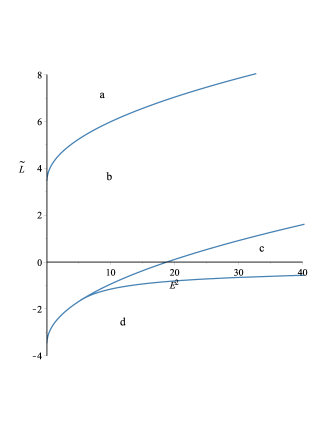
Figure 5: $\epsilon=1$, $\tilde{a}=0.8$, $\tilde{K}=12$,: Parametric $\tilde{L}$-$E^{2}$-diagram for the function $\tilde{\Theta}$. $\tilde{\Theta}$ possesses one zero in region b and two zeros in region c. In the a and d areas geodesic motion is not possible.

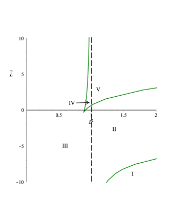
Figure 6: $\epsilon=1$, $\tilde{a}=0.8$, $\tilde{K}=12$,: Parametric $\tilde{L}$-$E^{2}$-diagram of the $\tilde{r}$-motion. The polynomial $\tilde{R}$ has 0 zero in region I, 2 zeros in region II, 2 positive zeros in region III, 4 positive zeros in region IV, 3 positive and 1 negative zeros in region V.

III.3 Analytical solution of geodesic equations

In this section, the analytical solutions of the geodesic equations (73)–(103), in Rotating Kerr-Sen Dilaton-Axion black hole spacetime, are presented in the terms of the elliptic Weierstrass $\wp$, $\zeta$ and $\sigma$ functions. Each equation will be treated separately.

III.3.1 r motion

The differential equation that describes the dynamics of $r$ Eq.(73)

$$\left(\dfrac{d\tilde{r}}{d\gamma}\right)^{2}=-\Delta_{\tilde{r}}(\tilde{K}+\varepsilon\tilde{r}(\tilde{r}+\tilde{r}_{\alpha}))+\left((\tilde{a}^{2}+\tilde{r}(\tilde{r}+\tilde{r}_{\alpha}))E-\tilde{a}\tilde{L}\right)^{2}=\tilde{R}(\tilde{r}),$$ (85)

is a polynomial of degree four for both $\varepsilon=1$ and $\varepsilon=0$ and, therefore, it is of elliptic type if $\tilde{R}(\tilde{r})$ has only simple zeros. With the substitutions $\tilde{r}=u^{-1}+\tilde{r}_{\tilde{R}}$ , where $\tilde{r}_{\tilde{R}}$ is a zero of $\tilde{R}$, transforms the problem to

$$(\dfrac{du}{d\varphi})^{2}=R_{3}(u)=\sum_{j=1}^{3}a_{j}u^{j},\qquad u(\varphi_{0})=u_{0},$$ (86)

with a polynomial $R_{3}$ of degree 3. Where

$$a_{j}=\dfrac{1}{(4-j)!}\dfrac{d^{(4-j)}R}{d\tilde{r}^{(4-j)}}(\tilde{r}_{R}).$$ (87)

Afterward, the substitution $u=\frac{1}{a_{3}}(4y-\frac{a_{2}}{3})$, implies

$$(\dfrac{dy}{d\gamma})^{2}=4y^{3}-g_{2}y-g_{3},$$ (88)

where

$$g_{2}=\frac{1}{16}\big{(}\frac{4}{3}a_{2}^{2}-4a_{1}a_{3}\big{)},$$ (89)

$$g_{3}=\frac{1}{16}\big{(}\frac{1}{3}a_{1}a_{2}a_{3}-\frac{2}{27}a_{2}^{3}-a_{0}a_{3}^{2}\big{)},$$ (90)

are the Weierstrass invariants. the differential equation (88), is elliptic of first kind, which can be solved by

$$y(\gamma)=\wp\big{(}\gamma-\gamma_{\theta,in};g_{2},g_{3}\big{)}.$$ (91)

Accordingly, the solution of Eq.(74), is given by

$$\tilde{r}(\gamma)=\dfrac{a_{3}}{4\wp(\gamma-\gamma_{\tilde{r},in};g_{2},g_{3})-\frac{a_{2}}{3}}+\tilde{r}_{\tilde{R}},$$ (92)

where, $\gamma_{\tilde{r},in}=\gamma_{0}+\int_{y_{0}}^{\infty}\dfrac{dy^{\prime}}{\sqrt{4y^{\prime 3}-g_{2}y^{\prime}-g_{3}}}$ , with $y_{0}=\frac{a_{3}}{4(\tilde{r}_{0}-r_{R})}+\frac{a_{2}}{12}$ , depends only on the initial values $\gamma_{0}$ and $\tilde{r}_{0}$ .

III.3.2 $\theta$ motion

The differential equation (74),

$$(\dfrac{d\theta}{d\gamma})^{2}=\tilde{\Theta}(\theta)=(\tilde{K}-\varepsilon\tilde{a}^{2}\cos^{2}\theta)-\dfrac{1}{\sin^{2}\theta}\big{(}\tilde{a}E\sin^{2}\theta-\tilde{L}\Xi\big{)}^{2},$$ (93)

which can be simplified by the substitution $\upsilon=cos^{2}\theta$, yielding

$$(\dfrac{d\upsilon}{d\gamma})^{2}=4\upsilon\tilde{\Theta}^{{}^{\prime}}({\upsilon})=4\upsilon(1-\upsilon)(\tilde{K}-\varepsilon\tilde{a}^{2}\upsilon)-4\upsilon\big{(}\tilde{a}E(1-\upsilon)-\tilde{L}\Xi\big{)}^{2}.$$ (94)

where, $\tilde{\Theta}^{{}^{\prime}}({\upsilon})=(1-\upsilon)\tilde{\Theta}({\upsilon})$ . The differential equation (94), for both $\varepsilon=1$ and $\varepsilon=0$, is a polynomial of degree three and with assume that $\tilde{\Theta}^{{}^{\prime}}({\upsilon})$ has only simple zeros, Then it can be solved in terms of the Weierstrass $\wp$ elliptic function. Thus, with the standard substitution $\upsilon=\frac{1}{b_{3}}\big{(}4y-\frac{b_{2}}{3}\big{)}$, where $4\upsilon\tilde{\Theta}^{{}^{\prime}}({\upsilon})=\sum_{i=1}^{3}b_{i}\upsilon^{i}$, transforms the problem to the form Eq.(88). The solution is then given by

$$\theta\big{(}\gamma\big{)}=\arccos\Big{(}\pm\sqrt{\frac{4}{b_{3}}\wp(\gamma-\gamma_{\theta,in};g_{2},g_{3})-\frac{b_{2}}{3b_{3}}}\Big{)},$$ (95)

where, $\gamma_{\theta,in}=\gamma_{0}+\int_{y_{0}}^{\infty}\dfrac{dy^{\prime}}{\sqrt{4y^{\prime 3}-g_{2}y^{\prime}-g_{3}}}$ , with $y_{0}=\dfrac{b_{3}}{4\cos^{2}(\theta_{0})}+\dfrac{b_{2}}{12}$ , depends on the initial values $\gamma_{0}$ and $\theta_{0}$ only. The sign of the square root depends on whether $\theta(\gamma)$, should be in $(0,\frac{\pi}{2})$ (positive sign) or in $(\frac{\pi}{2},\pi)$ (negative sign), and reflects the symmetry of the $\theta$ motion with respect to the equatorial plane $\theta=\frac{\pi}{2}$.

III.3.3 $\varphi$ motion

In this part and next part, we solve equation of $\varphi$ and $t$ motion according to Weierstrass $\wp$, $\zeta$ and $\sigma$ functions. For analysis $\varphi$ motion, we use Eq.(75),

$$(\dfrac{d\varphi}{d\gamma})=\dfrac{E(\tilde{a}^{3}+\tilde{r}(\tilde{r}+\tilde{r}_{\alpha})\tilde{a})-\tilde{L}\tilde{a}^{2}}{\Delta_{\tilde{r}}}-\dfrac{1}{\sin^{2}\theta}\big{(}\tilde{a}E\sin^{2}\theta-\tilde{L}\big{)}.$$ (96)

This equation can be splitted in a part dependent only on $\tilde{r}$ and in a part only dependent on $\theta$. Integration yields

$$\varphi-\varphi_{0}=\bigg{[}\int_{\gamma_{0}}^{\gamma}\dfrac{E(\tilde{a}^{3}+\tilde{r}(\tilde{r}+\tilde{r}_{\alpha})\tilde{a})-\tilde{L}\tilde{a}^{2}}{\Delta_{\tilde{r}(\gamma)}}d\gamma-\int_{\gamma_{0}}^{\gamma}\dfrac{\tilde{a}E\sin^{2}\theta-\tilde{L}}{\sin^{2}\theta(\gamma)}d\gamma\bigg{]}$$

$$=\bigg{[}\int_{\tilde{r}_{0}}^{\tilde{r}}\dfrac{E(\tilde{a}^{3}+\tilde{r}^{2}\tilde{a})-\tilde{L}\tilde{a}^{2}}{\Delta_{\tilde{r}}\sqrt{\tilde{R}}}d\tilde{r}-\int_{\theta_{0}}^{\theta}\dfrac{\tilde{a}E\sin^{2}\theta-\tilde{L}}{\sin^{2}\theta\sqrt{\tilde{\Theta}(\theta)}}d\theta\bigg{]}$$

$$=\bigg{[}\tilde{I}_{r}-\tilde{I}_{\theta}\bigg{]},$$ (97)

where, we substituted $\tilde{r}=\tilde{r}(\gamma)$, i.e. $\frac{d\tilde{r}}{d\gamma}=\sqrt{\tilde{R}}$, in the first and $\theta=\theta(\gamma)$, i.e. $\frac{d\theta}{d\gamma}=\sqrt{\tilde{\Theta}(\theta)}$, in the second integral. We will solve now the two integrals in Eq.(III.3.3) separately. Let us consider the integral

$$I_{\theta}=\int_{\theta_{0}}^{\theta}\dfrac{(\tilde{a}E\sin^{2}\theta-\tilde{L})d\theta}{\sin^{2}\theta\sqrt{\tilde{\Theta}(\theta)}},$$ (98)

which can be transformed to the simpler form

$$I_{\theta}=\mp\int_{\upsilon_{0}}^{\upsilon}\dfrac{\tilde{a}E(1-\upsilon)-\tilde{L}}{(1-\upsilon)\sqrt{4\upsilon\tilde{\Theta}^{{}^{\prime}}({\upsilon})}}d\upsilon^{\prime},$$ (99)

by the substitution $\upsilon=\cos^{2}\theta$, where $\tilde{\Theta}_{\upsilon}$, is defined in (81). Here, we have to pay special attention to the integration path. If $\theta\in(0,\frac{\pi}{2}]$, we have $\cos\theta=+\sqrt{\upsilon}$ but for $\theta\in[\frac{\pi}{2},\pi)$, then $\cos\theta=-\sqrt{\upsilon}$. Accordingly, we first have to split the integration path from $\theta_{0}$ to $\theta$ such that every piece is fully contained in the interval $(0,\frac{\pi}{2}]$, or $[\frac{\pi}{2},\pi)$, and then to choose the appropriate sign of the square root of $\upsilon$. In the following we assume for simplicity that $\cos\theta=+\sqrt{\upsilon}$. If $4\upsilon\tilde{\Theta_{\upsilon}}$ has only simple zeros, $I_{\theta}$ is of elliptic type and of third kind. We transform analogously to section (III.3.2), to the standard Weierstrass form by $\upsilon=\frac{1}{a_{3}}(4y-\frac{a_{2}}{3})$. Then, the solution to $I_{\theta}$, is given by

$$I_{\theta}=-\dfrac{\mid b_{3}\mid}{b_{3}}\bigg{\{}(\tilde{a}E)(\gamma-\gamma_{0})+\sum_{i=1}^{4}\dfrac{b_{3}\tilde{L}}{4\wp^{\prime}(\upsilon_{i})}\bigg{(}\zeta(\upsilon_{i})(\gamma-\gamma_{0})$$

$$+\log\dfrac{\sigma(\gamma-\gamma_{i})}{\sigma(\gamma_{0}-\gamma_{i})}\bigg{)}\bigg{\}},$$ (100)

where, the constants $b_{i}$, are defined as in section (III.3.2), $\wp=\wp(\gamma)=\gamma-\gamma_{\theta,in}$, and $\gamma_{0}=\wp(\gamma_{0})$ Hackmann:2010zz .

Now, we solve the $\tilde{r}$ dependent integral in (III.3.3),

$$I_{r}=\int_{\tilde{r}_{0}}^{\tilde{r}}\dfrac{E(\tilde{a}^{3}+\tilde{r}^{2}\tilde{a})-\tilde{L}\tilde{a}^{2}}{\Delta_{\tilde{r}}\sqrt{\tilde{R}}}d\tilde{r}.$$ (101)

If we consider that $\tilde{R}$, has only simple zeros, $I_{r}$ is of elliptic type and third kind. We transform analogously to section (III.3.1), to the standard Weierstrass form by $\tilde{r}=\pm 1/u+\tilde{r}_{\tilde{R}}$, with a zero $\tilde{r}_{\tilde{R}}$ of $\tilde{R}$, and then $u=\frac{1}{a_{3}}(4y-\frac{a_{2}}{3})$. Afterward, we simplify the integrand by a partial fraction decomposition and this integral can now be solved as

$$I_{r}(\gamma)=-\dfrac{\mid a_{3}\mid}{a_{3}}\bigg{\{}(\dfrac{E(\tilde{a}^{3}+\tilde{r}_{\tilde{R}}(\tilde{r}_{\tilde{R}}+\tilde{r}_{\alpha})\tilde{a})-\tilde{L}\tilde{a}^{2}}{\Delta_{\tilde{r}_{\tilde{R}}(\gamma)}})(\gamma-\gamma_{0})+\sum_{i,j=1}^{2}\dfrac{C_{i}}{\wp^{\prime}(\gamma_{ij})}\bigg{(}\zeta(\upsilon_{ij})(\gamma-\gamma_{0})$$

$$+\log\dfrac{\sigma(\gamma-\gamma_{ij})}{\sigma(\gamma_{0}-\gamma_{ij})}\bigg{)}\bigg{\}},$$ (102)

where, $\wp(\gamma_{ij}-\gamma_{r,in})=y_{i}$, and $C_{i}$, are the coefficients of the partial fractions $(y-y_{i})^{-1}$.

III.3.4 t motion

The equation for $t$ Eq.(103),

$$\left(\dfrac{d\tilde{t}}{d\gamma}\right)=\dfrac{(\tilde{a}^{2}+\tilde{r}(\tilde{r}+\tilde{r}_{\alpha})}{{\Delta_{\tilde{r}}}}\left((\tilde{a}^{2}+\tilde{r}(\tilde{r}+\tilde{r}_{\alpha}))E-\tilde{a}\tilde{L}\right)-a\big{(}\tilde{a}E\sin^{2}\theta-\tilde{L}\big{)},$$ (103)

has the same structure as the equation for the $\varphi$ motion. An integration yields

$$\tilde{t}-\tilde{t}_{0}=\bigg{[}\int_{\gamma_{0}}^{\gamma}{\dfrac{(\tilde{a}^{2}+\tilde{r}(\tilde{r}+\tilde{r}_{\alpha})}{{\Delta_{\tilde{r}}}}\left((\tilde{a}^{2}+\tilde{r}(\tilde{r}+\tilde{r}_{\alpha}))E-\tilde{a}\tilde{L}\right)}d\gamma-\int_{\gamma_{0}}^{\gamma}{a\big{(}\tilde{a}E\sin^{2}\theta-\tilde{L}\big{)}}$$

$$=\bigg{[}\tilde{I}_{r}-\tilde{a}\tilde{I}_{\theta}\bigg{]}.$$ (104)

Because we already demonstrated the solution procedure, we only give here the results for the most general cases. If $4\tilde{\Theta}_{\upsilon}$, where $\tilde{\Theta}_{\upsilon}$ is defined in Eq.(81), has only simple zeros the solution of the $\theta$ dependent part is given by

$$\tilde{I}_{\theta}=\dfrac{4\tilde{a}E}{b_{3}}\zeta(\gamma-\gamma_{0})+\dfrac{3\tilde{a}Eb_{3}+\tilde{a}Eb_{2}-3b_{3}\tilde{L}}{3b_{3}}(\gamma-\gamma_{0}).$$ (105)

And the solution of the $\tilde{r}$ dependent part is given by

$$I_{r}=C_{0}(\gamma-\gamma_{0})+\sum_{i=1}^{3}\sum_{j=1}^{2}\dfrac{C_{i1}\tilde{L}}{\wp^{{}^{\prime}}(\upsilon_{ij})}\bigg{(}\zeta(\upsilon_{ij})(\gamma-\gamma_{0})+\log\dfrac{\sigma(\gamma-\gamma_{ij})}{\sigma(\gamma_{0}-\gamma_{ij})}\bigg{)}$$

$$-\sum_{j=1}^{2}\dfrac{C_{32}\tilde{L}}{\wp^{{}^{\prime}}(\upsilon_{3j})}\bigg{(}\dfrac{\wp(\upsilon_{3j})\wp^{\prime}(\upsilon_{3j})+2\wp^{{}^{\prime\prime}}(\upsilon_{3j})\zeta(\upsilon_{3j})}{\wp^{{}^{\prime}}(\upsilon_{3j})^{2}}(\gamma-\gamma_{0})$$

$$+\zeta(\gamma-\gamma_{3j})+2\wp^{{}^{\prime\prime}}(\upsilon_{3j})\log\dfrac{\sigma(\gamma-\gamma_{3j})}{\sigma(\gamma_{0}-\gamma_{3j})}\bigg{)},$$ (106)

where, $C_{0}$, is a constant and $C_{ik}$ are the coefficients of the partial fractions $(y-y_{i})^{-k}$.

III.4 Orbits

Combination of Figs. 5 and 6 , is shown in Fig. 7. For each regions, examples of effective potentials are demonstrated in Fig. 8. With the help of the analytical solutions, the parametric $\tilde{L}$-$E^{2}$-diagrams and effective potentials, we can plot the orbits of test particles and light rays. Below we give a list of possible orbits. Let $\tilde{r}_{+}$ be the outer event horizon and $\tilde{r}_{-}$ be the inner horizon.

1. Transit orbit (TrO) with range $\tilde{r}\in(-\infty,\infty)$.

2. Escape orbit (EO) with range $\tilde{r}\in[r_{1},\infty)$ with $r_{1}>\tilde{r}_{+}$, or with range $\tilde{r}\in(-\infty,r_{1}]$ with $r_{1}<0$.

3. Two-world escape orbit (TEO) with range $[r_{1},\infty)$ where $0<r_{1}<r_{-}$.

4. Crossover two-world escape orbit (CTEO) with range $[r_{1},\infty)$ where $r_{1}<0$.

5. Bound orbit (BO) with range $\tilde{r}\in[r_{1},r_{2}]$ with

   1. $r_{1},r_{2}>r_{+}$, or

   2. $0<r_{1},r_{2}<r_{-}$.

6. Many-world bound orbit (MBO) with range $\tilde{r}\in[r_{1},r_{2}]$ where $0<r_{1}\leq r_{-}$ and $r_{2}\geq r_{+}$.

7. Terminating orbit (TO) with ranges either $\tilde{r}\in[0,\infty)$ or $\tilde{r}\in[0,r_{1}]$ with

   1. $r_{1}\geq\tilde{r}_{+}$, or

   2. $0<r_{1}<\tilde{r}_{-}$.

It should be noted that, the only way for a geodesic to reach the singularity (Terminating Orbit) is $\tilde{R}(\tilde{r}=0)=0$ and $\tilde{\Theta}(\theta=\frac{\pi}{2})=0$. This is the case if $\tilde{K}=(E\tilde{a}-\tilde{L})^{2}$.
A summary of possible orbit types can be found in Table 4.

Figure 9, shows two example plots of an escape orbit (a) and a two-world escape orbit (b), which crosses both horizons twice and escapes to another universe. A crossover two-world escape orbit, which crosses both horizons and $r=0$ and escapes to another universe, can be seen in Figure 10 (a). A Mani-world escape orbit which crosses both horizons several times, is depicted in 10 (b). In figure 11 (a) a bound orbit outside the both horizons is shown. Figure 11 (b) shows a many-world bound orbit, where both horizons are crossed several times.

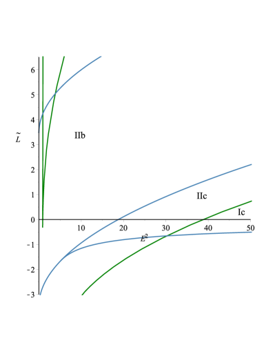
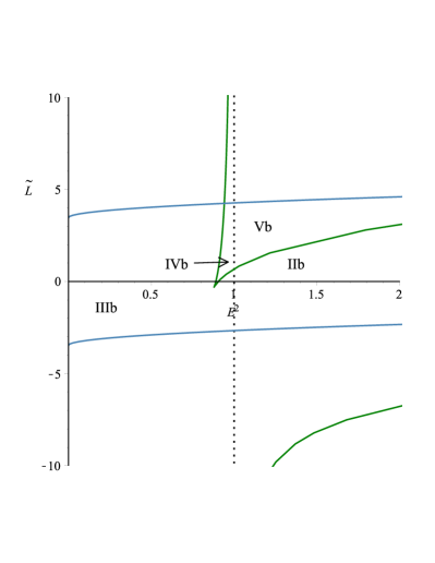
(a) closeup of figure (a)

Figure 7: $\epsilon=1$, $\tilde{a}=0.8$, $\tilde{K}=12$. Combined $\tilde{L}$-$E^{2}$-diagrams of the $\tilde{r}$-motion (green lines) and $\theta$-motion (blue lines). In regions marked with the letter b, the orbits cross $\theta=\frac{\pi}{2}$, but not $\tilde{r}=0$. Whereas in regions marked with the letter c, $\tilde{r}=0$ can be crossed but $\theta=\frac{\pi}{2}$ is never crossed.

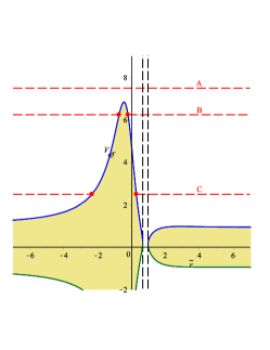
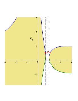
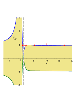
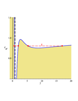
(a) closeup of figure (c)

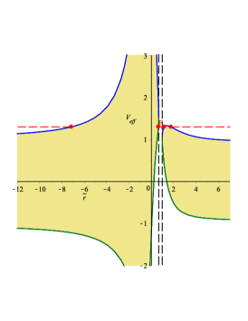
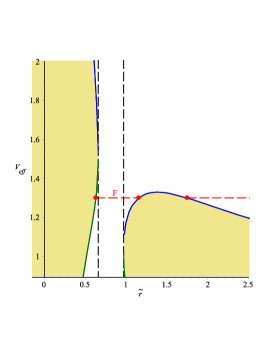
(b) closeup of figure (e)

Figure 8: Plots of the effective potential together with examples of energies for the different orbit types of table 4. The blue and green curves represent to the two branches of the effective potential. The red dashed lines correspond to energies. The red dots mark the zeros of the polynomial $R$, which are the turning points of the orbits. In the khaki area no motion is possible since $\tilde{R}<0$. The vertical black dashed lines show the position of the horizons. $\epsilon=1$, $\tilde{a}=0.8$, $\tilde{K}=12$, $\tilde{r}_{\alpha}=0.35$, and $\tilde{L}=0.35$, $\tilde{L}=0.45$, $\tilde{L}=0.5$, $\tilde{L}=2.5$, for (a), (b), (c) and (e) respectively.

type	zeros	region	range of $\tilde{r}$	orbit
A	0	Ic	(-4,-0.2)(3.5,0.2)[linewidth=0.5pt]-¿(-4,0)(3.5,0) [linewidth=0.5pt](-2.5,-0.2)(-2.5,0.2) [linewidth=0.5pt,doubleline=true](-0.5,-0.2)(-0.5,0.2) [linewidth=0.5pt,doubleline=true](1,-0.2)(1,0.2) [linewidth=1.2pt]-(-4,0)(3.5,0)	TrO
B	2	IIc	(-4,-0.2)(3.5,0.2)[linewidth=0.5pt]-¿(-4,0)(3.5,0) [linewidth=0.5pt](-2.5,-0.2)(-2.5,0.2) [linewidth=0.5pt,doubleline=true](-0.5,-0.2)(-0.5,0.2) [linewidth=0.5pt,doubleline=true](1,-0.2)(1,0.2) [linewidth=1.2pt]-*(-4,0)(-3.5,0) [linewidth=1.2pt]*-(-3,0)(3.5,0)	EO, CTEO
C	2	IIb	(-4,-0.2)(3.5,0.2)[linewidth=0.5pt]-¿(-4,0)(3.5,0) [linewidth=0.5pt](-2.5,-0.2)(-2.5,0.2) [linewidth=0.5pt,doubleline=true](-0.5,-0.2)(-0.5,0.2) [linewidth=0.5pt,doubleline=true](1,-0.2)(1,0.2) [linewidth=1.2pt]-*(-4,0)(-3,0) [linewidth=1.2pt]*-(-1.5,0)(3.5,0)	EO, TEO
D	2	IIIb	(-4,-0.2)(3.5,0.2)[linewidth=0.5pt]-¿(-4,0)(3.5,0) [linewidth=0.5pt](-2.5,-0.2)(-2.5,0.2) [linewidth=0.5pt,doubleline=true](-0.5,-0.2)(-0.5,0.2) [linewidth=0.5pt,doubleline=true](1,-0.2)(1,0.2) [linewidth=1.2pt]*-*(-0.5,0)(1.5,0)	TO/MBO
E	4	IVb	(-4,-0.2)(3.5,0.2)[linewidth=0.5pt]-¿(-4,0)(3.5,0) [linewidth=0.5pt](-2.5,-0.2)(-2.5,0.2) [linewidth=0.5pt,doubleline=true](-0.5,-0.2)(-0.5,0.2) [linewidth=0.5pt,doubleline=true](1,-0.2)(1,0.2) [linewidth=1.2pt]*-*(2,0)(3,0) [linewidth=1.2pt]*-*(-1,0)(1.5,0)	MBO, BO
F	4	Vb	(-4,-0.2)(3.5,0.2)[linewidth=0.5pt]-¿(-4,0)(3.5,0) [linewidth=0.5pt](-2.5,-0.2)(-2.5,0.2) [linewidth=0.5pt,doubleline=true](-0.5,-0.2)(-0.5,0.2) [linewidth=0.5pt,doubleline=true](1,-0.2)(1,0.2) [linewidth=1.2pt]-*(-4,0)(-3,0) [linewidth=1.2pt]*-*(-1,0)(1.5,0) [linewidth=1.2pt]*-(2,0)(3.5,0)	EO, MBO, EO

Table 4: Types of orbits in the spacetime of a rotating Kerr-Sen Dilaton-Axion black hole. The range of the orbits is represented by thick lines. The dots show the turning points of the orbits. The positions of the horizons are marked by a vertical double line. The single vertical line indicates $\tilde{r}=0$.

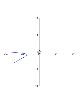
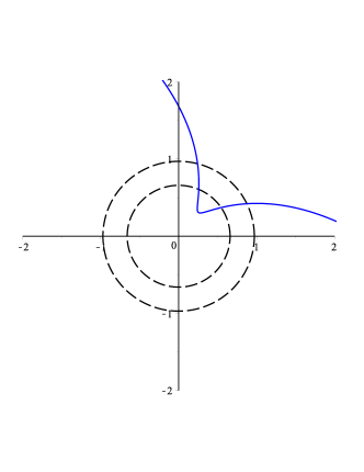
Figure 9: Two examples of possible orbits in the spacetime of a rotating Kerr-Sen Dilaton-Axion black hole. An escape orbit (a) and a two-world escape orbit (b), with parameters $\epsilon=1$, $\tilde{a}=0.8$, $\tilde{K}=12$, $\tilde{r}_{\alpha}=0.35$, $L=0.35$, $E=2.5$. The blue lines show the path of the orbits and the circles represents the event horizons.

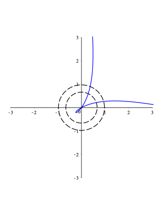
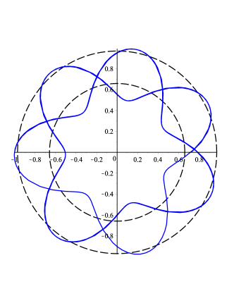
Figure 10: Two examples of possible orbits in the spacetime of a rotating Kerr-Sen Dilaton-Axion black hole. A crossover two-world escape orbit (a) and a Mani-world escape orbit (b), with parameters $\epsilon=1$, $\tilde{a}=0.8$, $\tilde{K}=12$, $\tilde{r}_{\alpha}=0.35$, $L=0.35$, $E=7.5$ and $L=0.5$, $E=0.5$ respectively. The blue lines show the path of the orbits and the circles represent the inner and outer horizons.

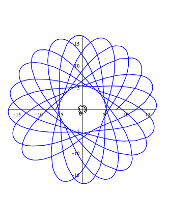
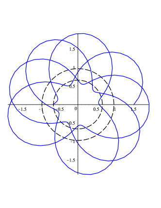
Figure 11: Two examples of possible orbits in the spacetime of a rotating Kerr-Sen Dilaton-Axion black hole. A Bound orbit (a) and a Many-world bound orbit (b), with parameters $\epsilon=1$, $\tilde{a}=0.8$, $\tilde{K}=12$, $\tilde{r}_{\alpha}=0.35$, $L=0.5$, $E=0.96$. The blue lines show the path of the orbits and the circles represent the inner and outer horizons.

IV CONCLUSIONS

In this paper, we considered the motion of test particles and light rays in the spacetime of the static (GMGHS, magnetically charged GMGHS and electrically charged GMGHS) and the rotating (Ker-Sen Dilaton-Axion ) dilaton black holes. We have derived geodesic equations of motion and classified them according to their energy $E$ and angular momentum $L$. The geodesic equations of motion can be solved in terms of the elliptic Weierstrass $\wp$, $\zeta$ and $\sigma$ functions. Possible types of orbits were derived using analytical solutions, effective potential techniques and parametric diagrams. For electrically charged GMGHS black hole, EO, TO and BO are possible, while for GMGHS and magnetically charged GMGHS black holes, EO, TEO, BO and MBO are possible and any type of terminating orbit are not possible for these metrics. Also, for rotating (Ker-Sen Dilaton-Axion) dilaton black hole, TrO, EO, TEO, CTEO, TO, BO and MBO are possible. Some observational phenomena such as the periastron shift of bound orbits and the deflection angle of light, are some results of these solutions. At the end of sec. II, we calculated such Astrophysical applications. Moreover, it would be interesting to use the results of this paper to study the shadow of dilaton black holes.

- (1) K. Schwarzschild, Sitzungsber. Preuss. Akad. Wiss. Berlin ( Math. Phys. ) 1916, 424 (1916) [physics/9912033].
- (2) C. Blaga, Serb. Astron. J. 190, 41 (2015) [arXiv:1407.1504 [gr-qc]].
- (3) G. W. Gibbons and K. i. Maeda, Nucl. Phys. B 298, 741 (1988).
- (4) D. Garfinkle, G. T. Horowitz and A. Strominger, Phys. Rev. D 43, 3140 (1991) [Phys. Rev. D 45, 3888 (1992)].
- (5) Mukherjee N. and Majumdar A.S., Gen. Rel. Grav. 39 583 (2007).
- (6) V. Faraoni, E. Gunzig and P. Nardone, Fund. Cosmic Phys. 20, 121 (1999) [gr-qc/9811047].
- (7) R. Casadio and B. Harms, Mod. Phys. Lett. A 14, 1089 (1999) [grqc/ 9806032].
- (8) Y. W. Kim, J. Choi, and Y. J. Park, Phys. Rev. D 89, 044004 (2014).
- (9) Y. Hagihara, Japan. J. Astron. Geophys, 8,67, (1931).
- (10) C. G. J. Jacobi, J. Reine Angew. Math. 22, 285 (1841) [Ostwald’s Klass. Exakt. Wiss. 77, 3 (1896)].
- (11) N.H. Abel. Oeuvres complètes de Niels Henrik Abel, (Christiania Imprimerie De Grondahl and Son, 1881).
- (12) B. Riemann. Crelle’s J., 54, 115 (1857).
- (13) B. Riemann. Crelle’s J., 65, 161 (1866).
- (14) K.T.W. Weierstrass. Crelle’s J., 47, 289 (1854).
- (15) H.F. Baker. Abelian Functions, Abel’s theorem and the allied theory of theta functions, (Cambridge University Press, Cambridge, 1995).
- (16) S. Chandrasekhar, The mathematical theory of black holes, (Clarendon press, Oxford, 1985).
- (17) E. Hackmann and C. Lammerzahl, Phys. Rev. D 78, 024035 (2008) [arXiv:1505.07973 [gr-qc]].
- (18) E. Hackmann, V. Kagramanova, J. Kunz and C. Lammerzahl, Phys. Rev. D 78, 124018 (2008); Phys. Rev. 79, 029901 (2009)(E) [arXiv:0812.2428 [gr-qc]].
- (19) E. Hackmann, C. Lammerzahl, V. Kagramanova and J. Kunz, Phys. Rev. D 81, 044020 (2010) [arXiv:1009.6117 [gr-qc]].
- (20) V. Kagramanova, J. Kunz, E. Hackmann and C. Lammerzahl, Phys. Rev. D 81, 124044 (2010) [arXiv:1002.4342 [gr-qc]].
- (21) E. Hackmann, B. Hartmann, C. Lammerzahl and P. Sirimachan, Phys. Rev. D 81, 064016 (2010) [arXiv:0912.2327 [gr-qc]].
- (22) E. Hackmann, B. Hartmann, C. Lammerzahl and P. Sirimachan, Phys. Rev. D 82, 044024 (2010) [arXiv:1006.1761 [gr-qc]].
- (23) S. Soroushfar, R. Saffari, J. Kunz and C. Lämmerzahl, Phys. Rev. D 92, [arXiv:1504.07854 [gr-qc]].
- (24) S. Soroushfar, R. Saffari and A. Jafari, [arXiv:1512.08449 [gr-qc]].
- (25) S. Fernando, Phys. Rev. D 85, 024033 (2012) [arXiv:1109.0254 [hep-th]].
- (26) M. Olivares and J. R. Villanueva, Eur. Phys. J. C 73, 2659 (2013) [arXiv:1311.4236 [gr-qc]].
- (27) P. P. Pradhan, Int. J. Mod. Phys. D 24, 1550086 (2015) [arXiv:1210.0221 [gr-qc]].
- (28) C. Blaga, Applications Math. 22, 41 (2013) [arXiv:1406.7421 [gr-qc]].
- (29) Harrison B.K, J. Math. Phys, 9, 1744-1752 (1968).
- (30) J. Choi, Mod. Phys. Lett. A 29, [arXiv:1407.6428 [gr-qc]].
- (31) W. Rindler and M. Ishak, Phys. Rev. D 76, 043006 (2007) [arXiv:0709.2948 [astro-ph]].
- (32) A. Bhattacharya, A. Panchenko, M. Scalia, C. Cattani and K. K. Nandi, JCAP 1009, 004 (2010) doi:10.1088/1475-7516/2010/09/004 [arXiv:0910.1112 [gr-qc]].
- (33) A. Bhattacharya, G. M. Garipova, E. Laserra, A. Bhadra and K. K. Nandi, JCAP 1102, 028 (2011) [arXiv:1002.2601 [gr-qc]].
- (34) G. V. Kraniotis and S. B. Whitehouse, Class. Quant. Grav. 20, 4817 (2003) [astro-ph/0305181].
- (35) G. V. Kraniotis, Class. Quant. Grav. 21, 4743 (2004) [gr-qc/0405095].
- (36) http://history.nasa.gov/SP-423/intro.htm.
- (37) A. Sen, Phys. Rev. Lett. 69, 1006 (1992) [hep-th/9204046].
- (38) S. Yazadjiev, Gen. Rel. Grav. 32, 2345 (2000) [gr-qc/9907092].
- (39) B. Carter, Phys. Rev. 174, 1559, (1968).
- (40) Y. Mino, Phys. Rev. D 67, 084027 (2003) [gr-qc/0302075].