A metric for sets of trajectories that is
practical and mathematically consistent
Abstract
Metrics on the space of sets of trajectories are important for scientists in the field of computer vision, machine learning, robotics, and general artificial intelligence. However, existing notions of closeness between sets of trajectories are either mathematically inconsistent or of limited practical use. In this paper, we outline the limitations in the current mathematically-consistent metrics, which are based on OSPA [1]; and the inconsistencies in the heuristic notions of closeness used in practice, whose main ideas are common to the CLEAR MOT measures [2] widely used in computer vision. In two steps, we then propose a new intuitive metric between sets of trajectories and address these limitations. First, we explain a solution that leads to a metric that is hard to compute. Then we modify this formulation to obtain a metric that is easy to compute while keeping the useful properties of the previous metric. Our notion of closeness is the first demonstrating the following three features: the metric 1) can be quickly computed, 2) incorporates confusion of trajectories’ identity in an optimal way, and 3) is a metric in the mathematical sense.
I Introduction
Similarity measures for sets of trajectories are very important. In computer vision, they are used to evaluate the performance of multi-object tracking algorithms. If and are the ground-truth and output trajectories of a tracker, a similarity measure can be used to distinguish a good tracker from a bad one, i.e. implies is a good tracker. In machine learning, algorithms such as [3, 4] and [5], can only cluster, classify and do a nearest neighbor search on sets of trajectories, if we have a similarity measure.
Given their importance, one would expect that existing widely-used measures would be easy to compute and would not produce counter-intuitive results. Surprisingly, this is not the case, leaving a critical problem unsolved.
The main limitation of most similarity measures is that they are not a mathematical metric. For example, the CLEAR MOT measures, widely used to evaluate the performance of trackers, are based on a heuristic and are not a metric. If a measure does not satisfy, for example, the triangle inequality (cf. Section III ), then we cannot guarantee that two good trackers (good according to this measure) produce similar outputs, which is counter-intuitive. In addition to this inconsistency, the CLEAR MOT also produce other counter-intuitive results (cf. Section VI). Furthermore, these results indirectly affect many other similarity measures that internally use the CLEAR MOT, or similar heuristics, to precompute an association between two sets of trajectories (e.g. [6, 7, 8, 9]).
However, even existing measures that are a metric, and that, we believe, are all variants of OSPA, can produce unreasonable results in simple scenarios (cf. Section II). We use OSPA-ST to refer to OSPA applied to sets of trajectories since it was not originally defined for this setting.
On the positive side, both the CLEAR MOT and the OSPA-based metrics are easy to define and have a computation time that scales well with the number and length of trajectories. These two attributes are part of the reason why the CLEAR MOT are popular.
In this paper we introduce the first measures that are simultaneously a mathematical metric, do not replicate the counter-intuitive results of OSPA-ST or CLEAR MOT and can also be quickly computed (cf. Section VII).
In the next section, we use an example to introduce the primary technical challenge in defining a measure for sets of trajectories and how this is addressed by OSPA-ST, the CLEAR MOT, and our metrics. We focus on OSPA-ST and the CLEAR MOT because they give a simple but powerful overview of the main ideas leading up to our work. We include a detailed list of related work in Section V.
II Main challenge: the association problem

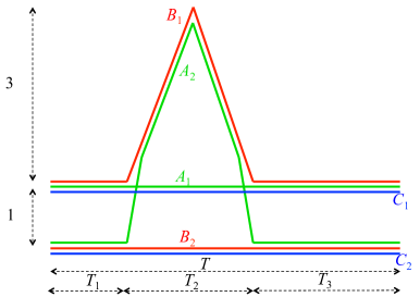
Figure 1 shows three sets of trajectories , and . Set has the ground truth trajectories of two people that start at a distance from each other and, twice, quickly exchange positions; and are the trajectories that two different tracking algorithms output. We represent time on the -axis (left to right) in frames and space on the -axis (top to bottom). For convenience, , and are normalized to sum to . We seek a distance measure for sets of trajectories to determine if (and/or ) is a good tracker.
If and only contained one trajectory, say and , we could define by computing the distance between and at each frame and returning the average distance over frames. Since this is not the case, the next idea is to define in two steps. Step 1: determine, for each frame, if we should compute the distance between and and between and or if we should compute the distance between and and between and . We refer to step 1 as finding an association between and . If, at a certain frame, we decide to compute the distance between and and between and , then we say that, at that frame, we associate with and with . Later, we formally define associations using permutations (See Section III). Step 2: given this association, compute the average distance between associated points.
The main problem in defining is to establish an association, i.e. step 1 above. Loosely speaking, typical approaches involve choosing an association that makes the average distance between associated points small. We can divide different approaches in three cases. The association between and (i) can change freely from frame to frame; (ii) cannot change; and (iii) can change from frame to frame but we pay a (smaller/higher) cost for (smaller/bigger) changes. We call this last cost a switching cost. We name the total (or average) distance between associated points the distance cost.
In (i), a “good tracker” tracks position accurately even if it does not track peoples’ identities (ID) correctly. At each frame, we associate to such that the sum of the distance between associated points is minimal. For Fig 1, we obtain an average distance between and (over frames and objects) that is and an average distance between and that is . Tracker is better than . Notice that from to track changes the person it is tracking. We call this as an identity switch.
In (ii), the tracker’s output must either be associated with for all frames or associated with for all frames. is associated with the other trajectory in . Between these two possibilities, we again choose the one that minimizes the average distance (over frame and objects). Now and . Tracker can be as good as tracker (for ), which is counter-intuitive, because ’s output is never close to the ground-truth.
In (iii), a “good tracker” must trade off some position accuracy (distance cost) for some ID accuracy (switching cost). The switching cost penalizes identity switches. It is also evident that category (iii) includes (i) and (iii) as particular cases of extreme tradeoffs.
The most widely used measures fall in category (iii). In computer vision, the prototypical example is MOTP, one of the CLEAR MOT measures. At each frame, MOTP heuristically tries to maintain the association between and as close as possible to the association made in the previous frame. It makes corrections to the association only if the association created in the previous frame applied to the current frame produces distances between matched points that are larger than a certain threshold . In the first frame, MOTP uses the association that minimizes the total distance. (cf. Definition 7 in Appendix A for a formal definition). By changing this threshold one can have different results. We always have . If is small, then , because we switch association twice. However, if is large, , because we never change from the association made in the first frame. Unfortunately, this heuristic leads to MOTP not being a metric and to other counter-intuitive results (cf. Section VI). In addition, all metrics (based on OSPA) fall in category (ii) because their associations are fix in time. Thus, the applications where they produce intuitive results are limited. We give another example of how OSPA-ST can produce counter-intuitive results in Appendix D.
Like the CLEAR MOT, our measures fall in category (iii). However, ours do not compute the association between and heuristically or sequentially. Rather, we solve a global optimization problem such that the sum of the distance cost and the switching cost over all time frames is minimized. Thus we avoid counter-intuitive results and obtain a metric.
To appreciate the difference between optimizing associations globally or sequentially, notice that, for Figure 1, MOTP either does not change the association across frames or changes it twice, from to and from to . Regardless of , and , MOTP never considers changing association just once. This happens because MOTP uses a fixed threshold to decide when to change associations. Hence, it fails to explore possibly better ways in which to compare and .
III Setup and notation
We denote the collection of all finite sets of finite trajectories by . We reserve the letters , and to represent finite sets of finite trajectories. is the trajectory in . Each trajectory is a finite set of time-state pairs with time and state . We focus on but it is possible to generalize our results to continuous time. We use to represent the state of the trajectory in at time .
When and are defined for all time instants and have the same number of trajectories, we can express using very simple notation. However, might not be defined for all values of . In addition, and might have a different number of trajectories. Thus, for mathematical convenience, we define a symbol and the following extension procedure.
Given and , we let and define and as follows. Let be the largest time index for which either or have trajectories with defined states. If , then, for all such that is defined, we set . Otherwise, . If then for all . We call these , -only trajectories. We define in the same way. Now and both have trajectories and their states are defined in the extended set for all . We call and extended sets of trajectories. Figure 2-(b) exemplifies this procedure. For example, agrees with for all except for for which is not defined and .
The meaning of an instant for which is not defined, i.e. , depends on the application, e.g. it might mean an occlusion. Other interpretations are possible, e.g., an object has yet to come into existence. We refrain for adhering to a particular interpretation of . Our use of resembles [10], where a null symbol is used.
We use to represent distance measures on . If , then measures the distance between and . The main goal of this work is to introduce mathematical metrics that are also easy to compute and produce intuitive results. Recall that, for any , a metric must satisfy the properties (i) (non-negativity) , (ii) (coincidence) iff , (iii) (symmetry) and (iv) (sub-additivity) .
Our definition of in the following sections needs two ingredients: an association between extended sets of trajectories and a distance between extended trajectories’ states.
We formally define an association between two sets of elements using permutations. A permutation is a bijective map from to itself. denotes the set of all permutations. We define the composition of as . is the inverse map of the bijection .
An association between and for which tells us that, to compute , we will use distances between the states of and the states of (See e.g. Def. 4). In this case, we say that associates trajectory to trajectory . Because computing might involve computing distances between different pairs of trajectories , at different points in time, we extend the terminology “association” to also mean a sequence of permutations. We define as the set of all length- sequences of associations. is the image of by the map . We define and . An association sequence between and for which tells us that, to compute , we will use the distance between and (See e.g. Def. 3). In this case, we say that associates the state to the state at time .
We use to indicate a distance between state elements. We define the extended distance such that for every we have (i) , (ii) and (iii) . Property (iii) guarantees that placeholders by themselves do not change the distance between and . Property (ii) defines a cost for comparing two states, one of which is not defined. For example, a larger might indicate a higher penalty for a missed or false track. Property (i) of is a technicality that makes be a metric. We define with element equal to .
In the context of computer vision tracking, having -only trajectories in , i.e. trajectories will all states equal to , and *-only trajectories in , allows two important types of associations.
| Symbols | Meaning |
|---|---|
| , | Set of trajectories and set of extended trajectories |
| , | State of trajectory in , and , at time |
| Symbol to mark states outside Euclidean space | |
| Set of all possible trajectories | |
| Distance between trajectory sets | |
| Distance between states and between extended states | |
| Cost between state * and state in Euclidean space | |
| Distance between extended states and | |
| Set of all possible permutations (perms.) | |
| , , | Permutation, its inverse, the image of by the map |
| , | Sequence of permutations, sequence of their inverses |
| The image of by the map in the sequence | |
| Set of all possible sequences of perms. of length | |
| Switching cost of permutation sequence | |
| Doubly stochastic matrix (d.s.m.), sequence of d.s.m. | |
| Entry of the d.s.m. of the sequence | |
| Set of all possible d.s.m. | |
| Set of all possible sequences of d.s.m. of length | |
| , , tr | Operators for matrix norm, transpose, trace |
In computing , we might not want to use any distance between a ground-truth trajectory in , say , and any reconstructed trajectories in . We get this by associating to a -only trajectory in . The points in are miss detections. A reconstructed trajectory, say , might not be related to any ground truth trajectories in . We represent this by associating to a -only trajectory in . is a spurious trajectory. To create the possibility that all ground truth trajectories might be missed and all tracker trajectories might be spurious, we need at least *-only trajectories in and *-only trajectories in .
With a particular application in mind, we might want to distinguish occlusions and no-target or penalize missed and false tracks differently. In this case, we might introduce multiple different placeholder symbols during the extension procedure, say and , and extend the definition of to penalize different symbol comparisons differently, e.g. , , , .
Not all interpretations and uses of these symbols make sense. Let be the output of a tracker and the ground truth. If has one -only trajectory, a miss detection, and has one -only trajectory, an always occluded object, then , even tough there is a cardinality error. This occurs because the meaning of in and is inconsistent. We could have used a different symbol for miss detections, , and occluded ground truth, . Furthermore, it is unreasonable to let always-hidden objects be part of the ground truth, i.e. let have one -only trajectory. Otherwise, a tracker is only good if it can find the number of objects behind a curtain.
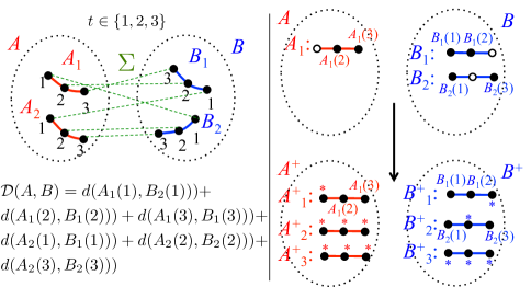
Figure 2-(a) illustrates how we can use an association between and and distance between state elements to define a distance . In Fig. 2-(a) we have dropped + for clarity. In this figure we have where , , .
In this paper we denote the set of doubly stochastic matrices as . We also define as the set of all length- sequences of doubly stochastic matrices.
Without specification, denotes the Euclidean norm, denotes the 1-norm, means transpose and tr matrix trace.
The above table gathers the most important notation used.
IV Proposed metrics
Here we introduce two novel families of metrics. We study their properties in Section VII.
Consider a map that gives a score, a switching cost, to sequences of associations and a map that computes distances between trajectories’ states. Recall that depends on ’s definition.
Definition 1.
The natural distance induced by and between two sets of trajectories is a map such that for any
| (1) |
A natural choice for is the Euclidian metric, that is, . One intuitive choice for is , , that basically counts the number of times we change association. We give other definitions for in Section VII.
Generally, computing is a combinatorially hard problem so we introduce a new metric that uses doubly stochastic matrices instead of permutations as associations between and 111By the Birkhoff–von Neumann theorem we know that is smallest convex set that contains all permutations (represented as permutation matrices).. Consider any norm on the space of matrices.
Definition 2.
The natural computable distance induced by and between two sets of trajectories is a map such that for any
| (2) |
A few important observations follow. First, notice that both measures minimize the sum of a distance cost plus a switching cost. Second, notice that we are defining a family of measures, not just two measures. Since , and are generic, our definitions can easily incorporate a scaling factor in front of each term of equations (1) and (2). Therefore, we can control the relative importance of the switching and distance costs.
Third, is a convex set and any norm is convex in , so computing amounts to solving a convex optimization problem, for which there are easy-to-use and efficient packages, e.g. CVX [11]. Later we show one choice of , among several, that reduces (2) to a linear program (LP). From this LP, we can approximate by forcing the variables to be in and then use techniques such as branch-and-bound, e.g. available in MATLAB and CPLEX.
Both and solve a global optimization problem to find the best tradeoff between distance cost and switching cost. As explained in Section II, this is in contrast to most measures used in practice such as MOTP, as explained below.
Definition 3.
The CLEAR MOT’s distance measure for evaluating tracking precision is called MOTP and is defined as
| (3) |
In the definition above, is the sequence of associations that CLEAR MOT builds heuristically (explained in Section II and formally in Appendix A).
We also know that and are more flexible than OSPA-ST, where associations cannot change with time. To see this, compare (1) and (2) with the definition of OSPA-ST below.
Definition 4.
The OSPA-ST metric is defined as
| (4) |
Our metrics include OSPA-ST as a particular case. Indeed, we recover OSPA-ST metric if we choose as: if , for some , and otherwise. In this case, we can compute in polynomial time, just like for OSPA-ST, using e.g. the Hungarian algorithm [12] (cf. [1]).
The doubly stochastic matrices of , can be transformed into permutations using a projection procedure that amounts to solving a LP. However, we cannot obtain doubly stochastic matrices from . We can use the associations from and to improve the computation of other heuristic measures of multi-target tracking performance, e.g. the number of ID switches or track purity.
Since , the -only trajectories add zero distance cost when associated with each other and so our metrics do not produce irrelevant switches between -only trajectories. In addition, although is a function of but not of and , when a particular application is in mind, we can have treat switches between different indices differently. We might, for instance, impose that confusing the ID of tracks and (e.g. different-team players) should be heavily penalized but confusing the ID of tracks and (e.g. same-team players) should not. Also, we can impose that a switch between a detected person and a , a non-detected person, should have a different cost than a switch between two detected persons.
Finally, using duality, and from now on using more compact matrix notation, we can equivalently define (cf. (2)) as
for some . Acting by analogy, can also be re-defined in a similar way. In other words, we do not need to worry about the sum of distance cost and switching cost.
V Related work
Except for our work, we found no similarity measure for sets of trajectories that is both mathematically consistent (a metric) and, at the same time, is useful and can deal with identity switches, i.e. it allows time-dependent associations. We focus our discussion around these characteristics. However, several of the ideas we review can be incorporated into our metrics to define new variants that compete with past work in settings not discussed, given the scope of this paper.
Our work is related to the general problem of defining a distance between two sets, however, this is a topic too vast to review in this paper alone. In [13], the reader can find many of those distances. In this article, the two sets and are sets of trajectories, and this limits the scope of our discussion. In the simplest case, when trajectories have only one vector, typical definitions compute an average or sum distance between all pairs of elements from and or just from a few pairs, e.g. [14]. Knowing which pairs to use when computing distances requires a procedure that matches elements of with elements of , e.g. [1, 15]. In general, however, each trajectory is composed of a set of vectors indexed by time, which limits our discussion even more.
To the best of our knowledge, the most rigorous works on metrics for sets of trajectories are based on [1]. In [1] the authors propose a distance for sets of vectors, the optimal sub-pattern assignment metric (OSPA), and explain its advantages over other distances in the context of multi-object filters. The OSPA metric has better sensitivity than the Hausdorff metric to cardinality differences between sets and does not lead to complicated interpretations as does the optimal mass transfer metric (OMAT) [16], proposed to address the limitations of the Hausdorff metric. OSPA, a metric for sets of vectors, can be defined from any distance between two vectors.
All the spin-offs of [1] focus on designing a metric for two sets of trajectories for the purpose of evaluating the performance of tracking algorithms. We recall however that, apart from tracking, many applications in machine learning and AI benefit if we work with a metric rather than a similarity measure that is not a metric. For example, the algorithms mentioned in the introduction [3, 4, 5] can only cluster, classify and find nearest neighbors if is a metric. None of the spin-offs of [1] allow associations that change with time and hence suffer from the same restricted applicability as OSPA (cf. Section II-(ii)).
The OSPA-T metric [10] for sets of trajectories is defined in two steps. First, we optimally match full tracks in to full tracks in while considering that tracks have different lengths and can be incomplete. Second, we assign labels to each track based on this match and compute the OSPA metric for each time using a new metric for pairs of vectors. uses both the vectors’ components and their labels. Finally, we sum the OSPA values across all time instants. Although the first step alone defines a metric, the authors in [17] point out that the full two-step procedure that describes OSPA-T is not a metric.
[17] defines the OSPAMT to be a metric and be more reliable than OSPA-T. The OSPAMT metric also optimally matches complete trajectories in to complete trajectories in but unlike OSPA-T allows us to match one trajectory in to multiple trajectories in (and vice-versa). The authors make this design choice to not penalize a tracker when it outputs only one track for two objects that move closely together.
Some extensions to OSPA incorporate measurement uncertainty. The Q-OSPA metric [18] weighs the distance between pairs of points by the product of their certainty and by adding a new term that is proportional to the product of the uncertainties. The H-OSPA metric [19] uses OSAP with distributions as states instead of vectors and uses the Hellinger distance between distributions instead of the Euclidean distance between vectors. Both works only allow sets that contain points, not trajectories. However, it is easy to combine them with [10] or [17] and get a metric for sets of trajectories.
The papers above are relatively recent, as is the search for mathematical metrics for sets of trajectories. However, researchers studying multi-object tracking have been using similarity measures for sets of trajectories to rank tracking algorithms for a while. Reviewing all the work done in this area is impossible. Especially because evaluating tracking performance has many challenges other than the problem of defining a similarity measure. See [20, 21] for some examples. Nonetheless, we mention various works that relate to our problem. We emphasize that none of the following works defines a metric mathematically.
Most of our paper is about finding an association between the elements in and (cf. Section II). In [22], which is expanded in [23], the authors are one of the first to identify this as the central problem in defining , although some of their ideas draw from the much earlier Ph.D. thesis of one of the authors [24]. They propose an one-to-one association between and but this association is optimally computed independently at every time instant. Also, there is no discussion about the number of association changes that might occur.
The CLEAR MOT are used widely in part because they allow control over the number of times that the association between and changes. It appears that [25] is one of the first that allow this. Like the CLEAR MOT, [25] uses a sequential matching procedure that tries to keep the association from the previous time instant if possible. The association that [25] uses at each time is not one-to-one optimal like in [22] or in the CLEAR MOT. Rather, the authors use a simple thresholding rule to decide which elements to associate. The idea of using a simple threshold rule to associate and has survived until relatively recently. For example, [26] match a full trajectory in to a whole trajectory in if they are close in space for a sufficiently long time interval. The authors in [27] use a similar thresholding rule.
Shortly after [22] and [23], some of the same authors discuss again the problem of associating to . [28] proposes four different methods for this problem. First: and are optimally matched independently at each time instant, possibly generating different associations at every time instant. Second: the association between and cannot change with time. Like in the OSPA-based metrics, this restricts the measure’s applicability (cf. Section II). Third: allow the association between and to change in time but only in special circumstances. Unfortunately, as they point out, this leads to an NP-hard problem. Fourth: use heuristics to minimize the number of changes in association. Some of these ideas resemble those used in the CLEAR MOT.
Measuring trackers’ performance is not just about defining similarity measures for sets of trajectories, or only concerned with establishing associations between and . If we have already matched the elements of and , which quantity should we compute from this match? A typical quantity that researchers calculate is the average or total distance between matched points. Our metrics are a combination of this quantity with the switching cost in the - association. Distance-related quantities apart, researchers also compute quality measures for the match itself, e.g. the number of trajectories in that do not match to any trajectory in (spurious tracks and missed tracks) or the number of times the match between and changes. Quantities like track purity and coalescence are often also computed once a match is established. [6, 7, 8] and [9] list many other measures of similarity between and and measures of quality for individual tracks.
It is worth mentioning a few non-mainstream works. [29] defines a distance based on comparing the occurrence of special discrete events in and . [30] proposes an information theoretic similarity measure. Finally, [31] proposes a similarity measure based on hidden Markov models to allow unequal temporal sampling rates in the trajectories.
VI Limitations of the CLEAR MOT
In the context of visual tracking, the next lemma shows that there are situations in which the average tracking distance cost over time gets arbitrarily close to zero with time while the CLEAR MOT produces an association that fails to see that. In other words, the CLEAR MOT can be counter-intuitive. Since none of the definitions of Section IV deal with time averages, in this section we use the following two definitions.
For any , we let
| (5) |
denote the empirical frequency of identity switches, i.e. association changes, where is the indicator function. Let
| (6) |
denote the average distance between and under . Note that, for example, .
Lema 1.
For any threshold , there exists trajectory sets and an association such that
The following lemma shows that, for any , the MOTP measure is mathematically inconsistent.
Lema 2.
MOTP is not a metric for any threshold .
The proofs of these two lemmas are in Appendix A.
It is also possible to prove that MOTA, the other widely used measure in the CLEAR MOT, does not define a metric. See www.jbento.info/papers/metriccompanion.pdf.
VII Properties of our metrics
The metrics we introduce do not produce the counter-intuitive results of OSPA-ST or MOTP because they control the tradeoff between switches and distances in a globally optimal way. In addition, we also show that they are a metric under mild conditions on , and .
Definition 5.
A map is a permutation measure if it satisfies the following three properties (i) if and only if is constant for some , (ii) and (iii) .
A few observations are in order. Clearly, if is a permutation measure so is . Also, property (iii) requires that all permutation matrices have the same dimensions, otherwise we cannot talk about their composition. In practice, this can be naturally achieved if e.g. all trajectories have a common maximum observation time , sets of trajectories have a common maximum number of trajectories , and permutation matrices have dimensions . Finally, Def. 5 implies that is invariant under reindexing. Indeed, by property (iii) followed by property (i) . On the other hand, by property (iii) followed by property (i) followed by property (ii) . Therefore, . A similar argument shows that . This invariance is part of the reason why we can later show that, under certain conditions, and are metrics.
One straightforward choice for is to count the number of times that the association between and changes.
Theorem 1.
Let . is a permutation measure.
Another two desirable choices for are (a) the function that sums the minimum number of transpositions to go from one permutation to the next and (b) the function that sums the number of adjacent transpositions to go from one permutation to the next. In what follows gives the minimum number of transpositions to obtain the identity permutation from and gives the number of adjacent transposition that the Bubble-Sort algorithm performs when sorting to obtain the identity permutation. The Cayley distance goes back to [32] and the Kendall distance to[33].
Theorem 2.
Let . is a permutation measure.
Although many intuitive choices for satisfy properties (i), (ii) and (iii) of Definition 5, some natural ones do not. For example, given a we might want to define as if and if (we can replace by some very large number if we want to be technical about the range of being ). This forces us not to create an association between and more intricate than a certain amount , something natural to desire. The following is proved in Appendix B.
Theorem 3.
does not satisfy (iii) in Definition 5. Thus, it is not a permutation measure.
The following theorem is similar to Theorem 3 and its proof is omitted.
Theorem 4.
Let . does not satisfy (iii) in Definition 5. Thus, it is not a permutation measure.
We now state our first main result.
Theorem 5.
If is a permutation measure and is a metric, then the map induced by them is a metric on .
Even if a function violates some of the properties in Definition 5, it could still induce a that is a metric. However, we often find that, from a set of associations and that violate Definition 5, we can build three sets of trajectories , and that violate some of the properties required of a metric. This is the case, for example, for induced by and equal to the Euclidean metric.
Theorem 6.
The map , induced by and the Euclidean distance , is not a metric.
The proof of this theorem is in Appendix B. In this sense, Definition 5 is required for to be a family of metrics.
We now focus on .
Definition 6.
A matrix norm is a switching norm if for any four matrices
| (7) |
The following Lemma gives sufficient conditions for a metric to satisfy property (7). See Appendix C for the proof.
Lema 3.
If is a sub-multiplicative norm and for all then is a switching norm.
This lemma implies, for example, that the 1-norm, -norm and spectral norm for matrices are valid choices for .
We now state our second most important result.
Theorem 7.
If is a switching norm and is a metric then the map induced by and is a metric on .
The proof of this theorem is in Appendix C.
The use of (matrix norm) in is extremely useful because it induces the changes of association to be sparse and, as the next theorem shows, reduces to solving a linear program. Recall that all LPs can be solved in polynomial time [34]. The theorem’s proof is in Appendix C.
Theorem 8.
For any , the metric induced by the matrix -norm and any can be computed (in polynomial time) by solving a linear program.
This LP can be a made sparse if we impose that for every such that and are distant we must have , i.e. we cannot associate distant points. Sparsity allows us to reduce the effective number of optimization variables in (2) and speedup computations further.
To end this section, let us explicitly include a scaling factor in the definition of . To be specific,
| (8) |
where, changing the definition of (5) and (6) in Section VI,
| (9) | ||||
| (10) |
If we compute for different ’s we obtain different pairs of values and . We can obtain more pairs of values if we compute and using as the permutation matrices representing the association produced by the CLEAR MOT or OSPA-ST. Even using MOTP alone, we can compute different values for and by changing .
If we fix and , we can display all these different pairs on a 2D scatter plot where each point is a pair evaluated on a different . Using such a scatter plot is a great way to assess the performance of a tracker on ground-truth under different similarity measures or when we do not know which or to use to compute and . For a fixed and , a good measure generates pairs closer to the origin. A very good measure generates pairs only on the Pareto frontier of this scatter plot. Not surprisingly, the pairs that produces for different values of generate this Pareto frontier. This follows from a well-known result in convex optimization theory that we state in Theorem 9 (see [35] for a proof). In this context, is the best metric we can hope. In particular, none of the examples where MOTP or OSPA-ST produce counter-intuitive results, like the counter example behind the proof of Lemma 1, lead to giving counter-intuitive results. The reader unfamiliar with convex optimization can jump to Section VIII.
Let be a convex set, e.g. , and let and be two convex functions in , e.g. and . Let . This set could be, for example, the points in our scatter plot plus points with worse costs. Let be the boundary of . Since is convex, is its Pareto frontier. For instance, could be the Pareto frontier we discussed above. Let be the curve of pairs generated by solving for different values of . This could be a tradeoff curve of pairs generated by for different ’s.
Theorem 9.
If then either for some or is a convex combination of and for some .
VIII Numerical results: computation time
In practice, there are many ways to compute , like when solving a convex optimization problem. To illustrate how easy it is to get code working, we have a simple Matlab code for in www.jbento.info/papers/metriccompanion.pdf. In the same document, we also have a simple Matlab code to estimate . However, to explore the limits of practical performance, we coded a non-trivial solver in C using , an implementation of the Alternating Direction Method of Multipliers (ADMM) that is available at github.com/parADMM/engine. has good performance in practice [36]. The ADMM is known to scale well, and its modular nature makes it easy to research future variants of without having to re-write much code. Furthermore, for strongly convex problems, its optimally-tuned convergence rate is as fast as that of the fastest first-order method [37].
[38] is a good introduction to the ADMM and its applications.
In Figure 3 we plot run-time in computing against the total duration of the input data for a different number of free association variables per time instant . We use the term “free association variables” because, as explained after Thm. 8, a few variables can be set to zero to sparsify the problem and save computation time. We choose the euclidean distance for and the one-norm for matrix norm in the switching cost. Similar run-times hold for other metrics. The run-time is computed for randomly generated and on a single core of a GHz Intel Core i5 MacBook Air. ADMM always converged to % accuracy in less than iterations.
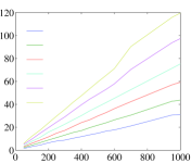
To interpret the plots, imagine we want to evaluate the quality of a tracker when tracking objects. Imagine that the tracker operates at frames per second and also that our tracker is noisy so that it produces a few false tracks that create approximately extra points per instant. To compute , and after we extend the ground-truth and hypothesis sets from and to and , we are dealing with distance matrices with about variables per instant . Using Fig. 3 we see that it take us about seconds to evaluate the accuracy of seconds of data. If we reduce the number of free variables per frame to half, e.g. by setting if is larger than a given threshold, then we can reduce the time to process secs. of data to about secs.
IX Numerical results: Optimal tradeoff curves
To the best of our knowledge, is the first measure that is a metric, can be computed in polynomial time and, in addition, deals with the tradeoff between distance cost and switching cost optimally. In this sense, (and future variants) is the best metric we can hope for (cf. Section VII).
To illustrate this optimal tradeoff, we build and compare tradeoff curves obtained from and MOTP. A tradeoff curve is a set of points where and are computed using (9) and (10). For , we obtain the different points along the curve by changing in (8). For MOTP we generate the tradeoff curve by changing . We do this for both synthetic and real data. We use the Euclidean metric for and the component-wise -norm for the matrix norm .
The direct interpretation of our results is that is better than MOTP. However, the important underlying fact is that builds better associations than (i) the heuristics widely used in the literature, e.g. the CLEAR MOT, and (ii) the optimal associations before our work that do not allow switches, e.g. OSPA-ST. Therefore, although we restrict the comparison to MOTP, we can show similar improvement over many measures that first establish a heuristic association between and . For example, Multiple Object Tracking Accuracy (MOTA), False Alarms per Frame, Ratio of Mostly Tracked trajectories, Ratio of Mostly Lost trajectories, the number of False Positives, number of False Negatives, number of ID Switches, the number of tracks Fragmentation and many of the measures listed in [7] and [9].
IX-A Real trackers and real data
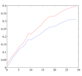
In Figure 4-(a) we show the performance of the trackers in [39] and [40] on the AVG-TownCentre data set. We call these trackers and respectively. The data set is part of the Multiple Object Tracking Benchmark [41] and is widely used in computer vision. It comes from a pedestrian street filmed from an elevated point for minutes and seconds and can be downloaded from http://www.robots.ox.ac.uk/ActiveVision/Research/Projects/2009bbenfold_headpose/project.html#datasets. In Figure 4-(b) we show the performance of the trackers in [42] and [43] on the PETS2009 data set, also part of the Multiple Object Tracking Benchmark. We call these trackers and respectively. Its duration is minute and seconds, and it can be downloaded from http://www.cvg.reading.ac.uk/PETS2009/a.html. More exact knowledge of these data sets and trackers is outside the scope of this paper. The point we want to make is in regard to comparing similarity measures. Not about comparing trackers’ performance on different data sets. We produced all the plots using the exact same output that each tracker produced in its respective paper, thanks to the authors who provided us with their trackers’ output. When coding , we set for AVG-TownCenter and for PETS2009.
As expected, the tradeoff curves from MOTP understate the performance of the trackers: all trackers are achieving a substantially smaller number of switches without incurring larger distance costs than what MOTP reports. Interestingly, for these trackers and data sets, keeps the same relative ordering of performance as MOTP. It is conceivable that there are situations in which a tracker is better than a tracker according to MOTP but not according to . It would be interesting to find such examples in future work.
IX-B Random ensemble of trajectories
Above, and are relatively close to each other because all the trackers are good trackers. In this section, we aim to study and that are more different. Hence, we use synthetic data to control the distance between and . We randomly generate with trajectories and make a distorted version of the trajectories in . The trajectories in have random start and end times and the objects in each trajectory randomly change their velocity’s direction along the way. The trajectories in are generated by randomly (i) fragmenting the trajectories in , (ii) removing some of the resulting trajectories, (iii) adding noise to all trajectories and (iv) flipping or not the ID of two trajectories if they pass by each other close enough. In the end, might have more or less than trajectories. In total, we have four knobs to increase or reduce the distance between and . These knobs are, (i) the amplitude of noise, ; (ii) the probability of fragmenting a track at each point in time, ; (iii) the probability of deleting a points in the track, ; and (iv) the threshold distance after which we allow to tracks ID to be switched or not randomly, .
Here, trajectories are far more diverse and complex than those in Section IX-A and in most publicly available real data sets. Real objects, like people, have relatively simple trajectories. In addition, we do not just test two data sets, like in Section IX-A. We generate data for about different configurations for each of the four knobs described above and for each of these configurations we generate random sets and . Hence, and in the context of computer vision tracking, it is as if we test different data sets of ground-truth and output trajectories.
We study the similarity between and using tradeoff plots with distance cost on the -axis and switching cost on the -axis. The smaller the area under the curve (AUC), the closer and are. In Fig. 5 we show the average AUC for and under different knob settings. Each AUC is normalized by the largest AUC possible. The largest AUC is the product of the largest distance cost possible with the largest switching cost possible. Each point in the plots is an average over random pairs and with the same knobs’ setting. In each plot we keep all but one knob constant.
As expected from Theorem 9, the AUC of is smaller than the AUC of MOTP. Note that it is incorrect to interpret these results as saying that MOTP is a scaled version of . We are computing exactly the same quantities for both measures: and according to (10) and (9). We just use a different for each measure. The curves of Figure 5 have a much deeper significance: they say that the conclusions that hold for real data hold in great generality, now in different tests and not just for two real data sets and four tackers as above. If we interpret and as the ground-truth and output of a tracker respectively, MOTP almost always says that the tracker is worse than what it really is. can see similarities between and that MOTP cannot.
X Conclusion
The problem of defining a similarity measure for sets of trajectories is crucial for computer vision, machine learning, and general AI. An essential aspect of this problem is finding a meaningful association between the elements of the sets. Existing measures that define useful associations fail to be a metric mathematically speaking, e.g., the CLEAR MOT. The ones that are a metric, only consider restrictive associations, i.e. associations that cannot change in time, e.g. OSPA-based metrics. is the first that simultaneously (1) is a metric, (2) allows time-dependent associations and hence can associate parts of trajectories to parts of trajectories, (3) allows controlling the complexity of this association in a globally optimal way and (4) has polynomial computation time.
The general idea of defining mathematical metrics for sets of trajectories using convex programs is our greatest overarching contribution. We are currently exploring variants of our metric that allow incorporating uncertainty, as well as richer comparisons between and without losing its useful properties. We are also exploring the use of this metric in a machine learning application for fast classification and retrieval of human actions/activities. We will present these extensions in future work.
References
- [1] D. Schuhmacher, B.-T. Vo, and B.-N. Vo, “A consistent metric for performance evaluation of multi-object filters,” Signal Processing, IEEE Trans. on, vol. 56, no. 8, pp. 3447–3457, 2008.
- [2] B. Keni and S. Rainer, “Evaluating multiple object tracking performance: the clear mot metrics,” EURASIP Journal on Image and Video Processing, vol. 2008, 2008.
- [3] V. Ganti, R. Ramakrishnan, J. Gehrke, A. Powell, and J. French, “Clustering large datasets in arbitrary metric spaces,” in Data Engineering, 1999. Proceedings., 15th Intern. Conf. on. IEEE, 1999, pp. 502–511.
- [4] J. Kleinberg and E. Tardos, “Approximation algorithms for classification problems with pairwise relationships: Metric labeling and markov random fields,” Journal of the ACM (JACM), vol. 49, 2002.
- [5] P. N. Yianilos, “Data structures and algorithms for nearest neighbor search in general metric spaces,” in Proceedings of the fourth annual ACM-SIAM Symposium on Discrete algorithms. Society for Industrial and Applied Mathematics, 1993, pp. 311–321.
- [6] S. S. Blackman, “Multiple-target tracking with radar applications,” Dedham, MA, Artech House, Inc., 1986, 463 p., vol. 1, 1986.
- [7] R. L. Rothrock and O. E. Drummond, “Performance metrics for multiple-sensor multiple-target tracking,” in AeroSense 2000. Intern. Society for Optics and Photonics, 2000, pp. 521–531.
- [8] Y. Bar-Shalom, X. R. Li, and T. Kirubarajan, Estimation with applications to tracking and navigation: theory algorithms and software. John Wiley & Sons, 2004.
- [9] A. A. Gorji, R. Tharmarasa, and T. Kirubarajan, “Performance measures for multiple target tracking problems,” in Information Fusion (FUSION), 2011 Proceedings of the 14th Intern. Conf. on. IEEE, 2011, pp. 1–8.
- [10] B. Ristic, B.-N. Vo, D. Clark, and B.-T. Vo, “A metric for performance evaluation of multi-target tracking algorithms,” Signal Processing, IEEE Trans. on, vol. 59, no. 7, pp. 3452–3457, 2011.
- [11] I. CVX Research, “CVX: Matlab software for disciplined convex programming, version 2.0,” http://cvxr.com/cvx, Aug. 2012.
- [12] H. W. Kuhn, “The hungarian method for the assignment problem,” Naval Research Logistics Quarterly, vol. 2, no. 1-2, pp. 83–97, 1955.
- [13] M. M. Deza and E. Deza, Encyclopedia of distances. Springer, 2009.
- [14] O. Fujita, “Metrics based on average distance between sets,” Japan Journal of Industrial and Applied Mathematics, vol. 30, 2013.
- [15] A. Gardner, J. Kanno, C. A. Duncan, and R. Selmic, “Measuring distance between unordered sets of different sizes,” in Computer Vision and Pattern Recognition (CVPR), 2014 IEEE Conf. on. IEEE, 2014.
- [16] J. R. Hoffman and R. P. Mahler, “Multitarget miss distance via optimal assignment,” Systems, Man and Cybernetics, Part A: Systems and Humans, IEEE Trans. on, vol. 34, no. 3, pp. 327–336, 2004.
- [17] T. Vu and R. Evans, “A new performance metric for multiple target tracking based on optimal subpattern assignment,” in Information Fusion (FUSION), 2014 17th Intern. Conf. on. IEEE, 2014, pp. 1–8.
- [18] H. Xiaofan, R. Tharmarasa, T. Kirubarajan, and T. Thayaparan, “A track quality based metric for evaluating performance of multitarget filters,” Aerospace and Electronic Systems, IEEE Trans. on, vol. 49, 2013.
- [19] S. Nagappa, D. E. Clark, and R. Mahler, “Incorporating track uncertainty into the ospa metric,” in Information Fusion (FUSION), 2011 Proceedings of the 14th Intern. Conf. on. IEEE, 2011, pp. 1–8.
- [20] T. Ellis, “Performance metrics and methods for tracking in surveillance,” in Proceedings of the 3rd IEEE Intern. Workshop on Performance Evaluation of Tracking and Surveillance (PETS02). Citeseer, 2002.
- [21] A. Milan, K. Schindler, and S. Roth, “Challenges of ground truth evaluation of multi-target tracking,” in Computer Vision and Pattern Recognition Workshops (CVPRW), 2013 IEEE Conf. on. IEEE, 2013.
- [22] B. E. Fridling and O. E. Drummond, “Performance evaluation methods for multiple-target-tracking algorithms,” in Orlando’91, Orlando, FL. Intern. Society for Optics and Photonics, 1991, pp. 371–383.
- [23] O. E. Drummond and B. E. Fridling, “Ambiguities in evaluating performance of multiple target tracking algorithms,” in Aerospace Sensing. Intern. Society for Optics and Photonics, 1992, pp. 326–337.
- [24] O. E. Drummond, “Multiple-object estimation,” 1975.
- [25] S. B. Colegrove, L. Davis, and S. J. Davey, “Performance assessment of tracking systems,” in Signal Processing and Its Applications, 1996. ISSPA 96., Fourth Intern. Symposium on. IEEE, 1996.
- [26] F. Yin, D. Makris, and S. A. Velastin, “Performance evaluation of object tracking algorithms,” in 10th IEEE Intern. Workshop on Performance Evaluation of Tracking and Surveillance (PETS2007), 2007.
- [27] F. Bashir and F. Porikli, “Performance evaluation of object detection and tracking systems,” in IEEE Intern. Workshop on Performance Evaluation of Tracking and Surveillance (PETS), vol. 5, 2006.
- [28] O. E. Drummond, “Methodologies for performance evaluation of multitarget multisensor tracking,” in SPIE’s Intern. Symposium on Optical Science, Engineering, and Instrumentation. Intern. Society for Optics and Photonics, 1999, pp. 355–369.
- [29] S. Pingali and J. Segen, “Performance evaluation of people tracking systems,” in Applications of Computer Vision, 1996. WACV’96., Proceedings 3rd IEEE Workshop on. IEEE, 1996, pp. 33–38.
- [30] K. K. Edward, P. D. Matthew, and B. H. Michael, “An information theoretic approach for tracker performance evaluation,” in Computer Vision, 2009 IEEE 12th Intern. Conf. on. IEEE, 2009, pp. 1523–1529.
- [31] F. Porikli, “Trajectory distance metric using hidden markov model based representation,” in IEEE European Conf. on Computer Vision, PETS Workshop, vol. 3, 2004.
- [32] A. Cayley, “Lxxvii. note on the theory of permutations,” The London, Edinburgh, and Dublin Philosophical Magazine and Journal of Science, vol. 34, no. 232, pp. 527–529, 1849.
- [33] M. G. Kendall, “A new measure of rank correlation,” Biometrika, pp. 81–93, 1938.
- [34] L. Khachiian, “Polynomial algorithm in linear programming,” in Akademiia Nauk SSSR, Doklady, vol. 244, 1979, pp. 1093–1096.
- [35] S. Boyd and L. Vandenberghe, Convex optimization. Cambridge university press, 2004.
- [36] N. Hao, A. Oghbaee, M. Rostami, N. Derbinsky, and J. Bento, “Testing fine-grained parallelism for the admm on a factor-graph,” arXiv preprint arXiv:1603.02526, 2016.
- [37] G. França and J. Bento, “An explicit rate bound for over-relaxed admm,” in 2016 IEEE International Symposium on Information Theory (ISIT). IEEE, 2016, pp. 2104–2108.
- [38] S. Boyd, N. Parikh, E. Chu, B. Peleato, and J. Eckstein, “Distributed optimization and statistical learning via the alternating direction method of multipliers,” Foundations and Trends® in Machine Learning, vol. 3, no. 1, pp. 1–122, 2011.
- [39] B. Benfold and I. Reid, “Guiding visual surveillance by tracking human attention.” in BMVC, 2009, pp. 1–11.
- [40] ——, “Stable multi-target tracking in real-time surveillance video,” in Computer Vision and Pattern Recognition (CVPR), 2011 IEEE Conf. on. IEEE, 2011, pp. 3457–3464.
- [41] “Multiple object tracking benchmark,” http://www.motchallenge.net, accessed: 2015-03-01.
- [42] B. Yang and R. Nevatia, “Multi-target tracking by online learning of non-linear motion patterns and robust appearance models,” in Computer Vision and Pattern Recognition (CVPR), 2012 IEEE Conf. on. IEEE, 2012, pp. 1918–1925.
- [43] F. Poiesi and A. Cavallaro, “Tracking multiple high-density homogeneous targets,” Circuits and Systems for Video Technology, IEEE Trans. on, vol. 25, no. 4, pp. 623–637, 2015.
Appendix A Theory on the limitations of the CLEAR MOT
Let us formally describe the heuristic used by the CLEAR MOT.
Definition 7.
The CLEAR MOT matching heuristic defines sequentially as follows.
-
1.
Initialize such that is minimal;
-
2.
For each do: for all such that and fix . We call such matches as anchored. Set the non-fixed components of such that is minimal.
Proof of Lemma 1.
We construct a validating example for any , with and , i.e. , and where and are 1D trajectories. We generalize this example to any and at the end.
Consider the two sets of one-dimensional trajectories and defined in Figure 6. Time is on the -axis (left to right) and space on the -axis (bottom to top). and are fixed. grows with .
Since we assume , the CLEAR MOT builds an association sequence that initially matches to but some time after matches to to minimize the distance between matched points. After , this last association is anchored given that . Hence,
The number of times that is , thus . For after , . Thus . However, if we choose , we have and . The result of the lemma follows.
To see that the proof holds for any , we extend and as follows. Without loss of generality, we assume is even. If the 1D trajectory above is equal to , define the 2D trajectory such that
where is a constant large enough such that trajectories for different ’s are not close to each other under the measure. We define similarly. Define
and similarly . In this setting, the bounds previously computed on and change by a factor of , while the bounds on and change by a factor of . Thus the statement of the lemma still holds.
To extend the proof for an odd , append to and two equal trajectories far away from all other trajectories such that they are matched to each other. They do not contribute to either or .
Finally, to see that the proof also holds for any , we rescale space-axis in Figure 6. This changes the bounds on by a factor of and leaves the bounds on unchanged, thus obtains the result. ∎
Proof of lemma 5.
We construct for which the triangle inequality is violated. Specifically, .
Without loss of generality, we assume . To see that the result holds for all , we employ the space-rescaling trick in the proof of Lemma 1.
Consider the sets , and as in Fig. 6, where the trajectories extend to some large . and are fixed. grows with . To make calculations simpler, we work with divided by in Def. 3.
Let us compute first. The association for this distance is because (i) we start with the association , (ii) at some point after we need to change the association to because the initial association exceeds and (iii) for times after the the association is anchored because . Therefore, .
Now we compute . The association for is because (i) we start with , (ii) the association is always anchored because the distance between and is always zero and thus always smaller than and (iii) after some point, when the distance between and exceeds , MOTP still keeps the association because and are already anchored. Under this association, numerical computation leads to . Similarly, .
Therefore, for large enough we have . ∎
Appendix B Properties of our metrics:
To prove Theorem 5, we need the following lemma.
Lema 4.
The map is a metric on .
Proof.
We verify that satisfies the four conditions of a metric. Let .
Non-negativity and symmetry are obvious.
To verify the coincidence property, observe that implies either or, since , . Because is a metric, this in turn implies that . In other words, .
To verify the subadditivity property, we need to consider eight different cases of the triangle inequality. We first consider the non-trivial cases. If , then
If and , then and
It is easy to check the other six cases. ∎
Proof of Theorem 5.
Let be three elements in . We verify the four conditions of a metric for .
Coincidence property: We show that if and only if . Recall that and are unordered sets of trajectories. Hence implies that there is an isomorphism between and . In other words, they are equal apart from a relabeling of the elements. If and we set then the function to minimize on the right-hand-side of equation (1) is equal to zero. This is an isomorphism between and . Since the minimum of (1) must always be non-negative, we conclude that . Conversely, assume that and let be a minimizer in (1). implies that . Therefore , for all and . Since the labeling of the trajectories does not affect the computation of , we assume without loss of generality that their labeling is such that we can write . also implies that, for all and , we have . Since is a metric, this in turn implies that for all and , which is the same as saying that . Hence . To be more specific, is equal to apart from a relabeling of its trajectories.
Symmetry property: Since only depends on and through we have .
Subadditivity property: We prove . First, notice that we can add any extra number of -only trajectories to , or without changing . Recall that is number of trajectories in , and . In this part of the proof, should be the sum of the cardinalities of the two sets of highest cardinality among , and . In Section III, was just the sum of the cardinalities of and . is the maximum time index observed in , and .
Since is a metric, we can write that
| (11) |
for any and for all and . Now notice that
Using this together with (B), we can write
Let us define where . This means . We can use to rewrite the expression above as
| (12) |
Using Definition 5, we can write
| (13) |
Finally, we find the minimum of both sides of the inequality over all pairs of and . Recall the relationship and the fact that we can choose independently of . Consequently,
Hence, . ∎
Proof of Theorem 1.
The first two properties of the permutation measure are trivial to verify. To verify the third property, it is sufficient to prove that
Since the left-hand-side is at most , we only need to consider the case in which the right-hand-side is less than , i.e.,
In this case, it follows that and . Consequently, the left-hand-side equals as well in this case. Hence the property is verified. ∎
Proof of Theorem 2.
The first two properties of the permutation measure are immediate to check from the definition of . To prove the third property it suffices to show that
To prove this we use of the following two facts.
Fact 1: if then . To see why this is true, notice that this inequality can be rewritten as where , and , the identity permutation. Then, it is basically saying that shortest set of transpositions that take to is smaller than any set of transpositions that first take to and then to .
Fact 2: if then . This is true because is just a relabeling of the permutation and is invariant to relabeling.
Let
Observe that the permutation satisfies
Finally, we can apply Fact 2 followed by Fact 1, and obtain (dropping Cayley for clarity).
∎
Proof of Theorem 3.
We give a counter example that violates property (iii) for . It is also easy to come up with similar counter examples that violate property (iii) for any value of . Let be the identity permutation and let be the permutation that swaps and . Let and let . We have and but . ∎
Proof of Theorem 6.
We provide a special case where the triangle inequality is violated. Let , and be three sets of trajectories. We assume , but it is easy to change , and such that the proof holds for any ,222It is easy to see that we do not in fact need to be the Euclidean distance for the proof to hold.. Let be the identity permutation and let be the permutation that swaps and . Let , , , where
Now consider equation (1) with and . The optimization problem for ,
has a minimum of at . We can see this because forces us to either do one switch only or no switch at all. Doing no switch at all makes us incur a cost larger than in the distance term. Similarly, the optimization problem for has a minimum of at . When we solve the optimization problem for , we are only allowed to perform one change in the association between and , otherwise the term makes us pay a very large cost. With only one change in the association, we incur a distance of for or or . Hence, . ∎
Appendix C Properties of our metrics:
Proof of Theorem 7.
Let and be any elements of .
Coincidence property: If ,
then for all . Hence, for all such that
. Recall that if is a doubly stochastic matrix, then there exists a permutation , such that
for all . Therefore, for all and . In other words,
and are identical apart from a relabeling of their elements.
Symmetry property: Using the properties of trace, we have
Minimizing with respect to is the same as minimizing with
respect to . Thus .
Subadditivity property: We prove that
.
First, notice that we can add any extra number of -only trajectories to , or without changing . Recall that is number of trajectories in , and . In this part of the proof, should be the sum of the cardinalities of the two sets of highest cardinality among , and . In Section III, was just the sum of the cardinalities of and . is the maximum time index observed in , and .
First note that, since is a metric we have that for any . Let and . We multiply both sides of the previous inequality by and sum over to obtain
where we omitted in and . Since , we have and . To simplify this expression, and again omitting in and , we re-write the previous inequality in matrix notation as
From our assumption on (c.f. Property (7)), we have
Adding the last two inequalities, summing over and minimizing over we have
Note that for any , we have . Therefore, in the minimization performed on the left hand side, we can replace by a single . The subadditivity property follows. ∎
Proof of Lemma 3.
Let , whose norms are less than .
The third inequality above is obtained using sub-multiplicity. ∎
Proof of Theorem 8.
The constraints which define are a set of linear constraints. In addition, the first term in the objective is a linear function of . Notice also that we can replace the term in the objective by , if we add the additional constraints that for all . We can also represent these additional constraints as linear constraints. Specifically, since
each of these constraints can be replaced by for all and if we add the additional constraints
for all , and . Each of these constraints can be replaced two linear constraints, namely
∎
Appendix D Some extra observations
In this section make some extra observations that are not essential to understand what was presented above. We use the same setup and notation as explained in Section III of the main paper.
Another example of OSPA-ST producing counter-intuitive results
Consider the setup in Figure 7 where two people, and , pass by each other and two trackers, and , produce output trajectories , , and . Space is measure on the -axis (bottom to top) and time on the -axis (left to right). To aid visualization, close lines should be considered on top of each other.
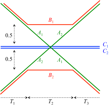
Let . By symmetry and the fact that OSPA-ST does not allow associations that change with time we can assume without loss of generality that in computing OSPA-ST associates to and to and that in computing OSPA-ST associates to and to .
If , the average distance between and can be arbitrarily close to the average distance between and . More formally, as . In other words, OSPA-ST says that tracker is as good as tracker while our intuition says that is the better tracker. produces good tracks for most of the time and simply makes an identity switch during internval . On the other hand, is a trivial tracker that always outputs regardless of the input.
MOTA does not define a metric
First recall how to compute MOTA between two sets of trajectories and . First compute the CLEAR MOT association between and as described in Appendix A. Second, compute a positive linear combination, , of three quantities , and where: is the number of changes of association between trajectories; is the number of points of trajectories in unassociated to any point in ; and is the number of points of trajectories in unassociated to any point in . MOTA is defined as but since distances must decrease as and get similar we define .
Lema 5.
is not a metric for any threshold or positive linear combination used to define .
Proof.
We given an example of three sets , and such while , hence the triangle inequality is violated. Our counter example works for but by scaling space we can prove the lemma for any .
Consider , and as in Figure 1 in the main paper, which we reproduce here for convenience. To aid visualization, close lines should be considered on top of each other and transitions in almost instantaneous. Time is on the -axis (left to right) and space is on the -axis (bottom to top).
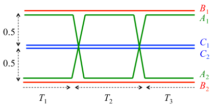
When we compute , associates to and to for all times . (we can interchange and since they are equal). There are no changes in association because the distances computed are always less than and , thus . In addition, there are no unallocated tracks so . Therefore regardless of the coefficients in the linear combination . Similarly we get .
When we compute we find the following: before , associates to ; after and before , the distance between and becomes and so changes association and matches to . After , the distance between and becomes and so changes association back to matches to . We change association twice and so We just focused on who matches to. The remaining tracks are matched to each other so . In short .
∎