Abstract

The linear time-dependent constants of motion of the parametric amplifier are obtained and used to determine in the tomographic-probability representation the evolution of a general two-mode Gaussian state. By means of the discretization of the continuous variable density matrix, the von Neumann and linear entropies are calculated to measure the entanglement properties between the modes of the amplifier. The obtained results for the nonlocal correlations are compared with those associated to a linear map of discretized symplectic Gaussian-state tomogram onto a qubit tomogram. This qubit portrait procedure is used to establish Bell-type’s inequalities, which provide a necessary condition to determine the separability of quantum states, which can be evaluated through homodyne detection. Other no-signaling nonlocal correlations are defined through the portrait procedure for noncomposite systems.

Keywords: parametric amplifier, quantum entanglement, Gaussian states, Bell inequalities, probability representation.

1 Introduction

The linear time-dependent invariants of multidimensional quadratic Hamiltonians in the position and momentum operators have been the subject of many research studies [1, 2, 3, 4, 5]. These constants of motion are useful to determine the propagators of the Hamiltonian systems and thus to study time-dependent problems in quantum mechanics. It has been shown that these propagators can be also obtained via the path integral formulation of quantum mechanics [6].

There are many specific systems of physical interest described by quadratic Hamiltonians, such as the parametric amplifier [7, 8], and others used in circuit electrodynamics based on the Josephson junction technique [9, 10, 11].

The tomographic probability representation introduced in 1996 is a generalization of the optical tomography scheme [12]. In this new formulation of quantum mechanics, the states are described by measurable positive probabilities.

In 1935, EPR and Schrödinger defined the entanglement concept as a strange phenomena [13, 14]. In the sixties, Bell [15] and Clauser–Horne–Shimony–Holt (CHSH) [16] established that the predictions of quantum theory cannot be accounted by any local theory. In a typical Bell experiment [17], it has been established an inequality valid for separable states of a bipartite system with the bound 2. An experimental check of the violation of the Bell–CHSH inequality with the bound 2 was first performed in [18]. Since the nineties the entanglement properties of a quantum system have been used as a resource to do tasks as quantum cryptography, quantum teleportation, and measurements in quantum computation. These facts lead to the growing interest in the identification of the quantum correlations or in the non-local behaviour of the quantum physics [17, 19]. The bound 2 of the Bell–CHSH inequality can be violated for entangled states of a composite system, which exhibit strong correlations of the subsystems. The paradigmatic upper bound of the CHSH inequality $2\sqrt{2}$ was proved by Cirelson [20] for quantum correlations in a bipartite system. On the other hand, formally there exists even an upper bound 4 discussed in [21], which corresponds to superquantum correlations in the systems modeling some properties of two-qubit states. A tomographic approach to test the nonlocality was proposed for the description of a correlated two-mode quantum state of light [22]. This proposal was implemented in [23] using a balanced homodyne detection on temporal modes of light, in which a clear violation of Bell’s inequality was found.

A qubit-portrait scheme of qudit tomograms has been proposed in [24], which allows one to discuss the Bell–CHSH inequality [15, 16, 25] for two qubits within the framework of the probability representation of quantum mechanics introduced in [12, 26]. It was also proposed that the necessary condition of separability of a bipartite qudit state is the separability of its qubit portrait [24]. This portrait method can be extended to photon-number tomograms with some modifications, which is useful to detect entanglement of two-mode light states. Specifically, the violation of the Bell–CHSH inequality indicates immediately that the state is entangled [27].

The models of the parametric amplifier and the frequency converter were proposed in [28] for two modes of the electromagnetic field, which represent the signal and idler photons. These harmonic oscillator modes are coupled by a classical field of frequency $\omega$ (referred as pump frequency) which may (or may not) satisfy the resonance condition [7, 29, 30], that is, $\omega=\omega_{a}+\omega_{b}$ for the parametric amplifier or $\omega=\omega_{a}-\omega_{b}$ for the frequency converter.

The model Hamiltonian [7] contains the main elements for the description of physical realizations of the parametric amplifier. As an example, we have a lossless nonlinear dielectric substance that couples the modes of a resonant cavity with reflecting walls [28]. In this case, there is a pump field oscillating with a frequency equal to the sum of the frequencies of the two modes, and it is strong enough to be represented in classical terms. The two-mode nonresonant parametric amplifier has been studied to find nonclassical features as revivals and squeezing in [7], where it was shown that the existence of quantum revivals is possible and the correlation effects are very sensitive to the form of the initial state of the system.

Recently, fiber optical parametric amplifiers have been developed with a total amplification of 60–70 dB over an input signal [31, 32]. Also the dynamics of the entanglement of Gaussian states of systems in a reservoir model has been studied in [33, 34]. The properties of superpositions of coherent states are presented in [35, 36]. A new resonant condition technique has been developed to determine experimentally the quadrature fluctuations of the light field, that is, the covariance matrix [37, 38, 39]. Thus, the operation of the parametric amplifier is sufficiently well understood. Nevertheless, the dynamical invariants of this system were not discussed in the literature, and one of the aims of this paper is to obtain and apply the special linear-in-quadrature time-dependent constants of motion of this amplifier.

In this work, we construct the linear time-dependent constants of motion of the nondegenerated parametric amplifier for the trigonometric and hyperbolic cases. Using these constants of motion we calculate, for the first time, the amplifier symplectic tomograms associated to the dynamics of Gaussian states. The other goal of this article is to propose a discretization method of the amplifier density matrices, which allow us to evaluate the von Neumann and linear entropies to measure the entanglement between the idler and signal modes of the amplifier. A portrait map of the symplectic tomogram onto a qubit is defined to explore possible sufficient conditions to have entanglement. For a noncomposite system, through the portrait picture, we show the possible existence of superquantum correlations i.e., the violation of the Cirelson bound.

The results presented could be of interest mainly in the context of theoretical and experimental researches in the fields of the theory of entanglement and Bell non-locality.

This paper is organized as follows.

The Hamiltonian for the parametric amplifier is defined in section 2, together with their analytic solution (trigonometric case) in terms of the corresponding linear time-dependent invariants. They are constructed for special conditions on the Hamiltonian parameters, and the other solution (hyperbolic case) can be obtained by analytic continuation. In section 3, the two-mode Green function is written in terms of the time-dependent symplectic matrix ($\boldsymbol{\Lambda}(t)$) and the corresponding two-mode Gaussian states at time $t$ are presented. The evolution of the covariance matrices are also calculated. The symplectic and optical tomograms are described in section 4, making use of the covariance matrices. In section 5, the von Neumann and linear entropies for the two-mode Gaussian state in the parametric amplifier are calculated using the discrete form of the two-mode density matrix and the corresponding reduced density matrix for the subsystem. The portrait of continuous symplectic and optical tomograms in the form of a two-qubit tomogram is determined in section 6. This portrait is used to define Bell-type inequalities that is a sufficient condition for separability, and a violation of this inequality is a necessary condition to entanglement. Also in this section non-Bell correlations within a noncomposite system are studied obtaining strong correlations even larger that the Cirelson bound $2\sqrt{2}$ [20]. In the final section, the conclusions are given, and some technical details are presented in Appendix A.

2 Hamiltonian and linear dynamical invariants for the parametric amplifier

The model of the parametric amplifier assumes that the two modes are described by harmonic oscillators of frequencies $\omega_{a}$ and $\omega_{b}$. The two modes are coupled by an oscillating parameter called the pump with frequency $\omega$, which may (or may not) satisfy the parametric resonance condition $\omega=\omega_{a}+\omega_{b}$ [29, 30, 7]. Therefore, the Hamiltonian can be written as

$$H=\hbar\omega_{a}a^{\dagger}a+\hbar\omega_{b}b^{\dagger}b-\hbar k\left(a^{\dagger}b^{\dagger}e^{-i\omega t}+abe^{i\omega t}\right)\,,$$ (1)

where $k=\chi^{(2)}\sqrt{I_{p}}/v$, with $v$ being the group velocity of the light in the medium, $\chi^{(2)}$ is the medium nonlinearity and $I_{p}$ is the intensity of the pump [40]. The sets $(a^{\dagger},a)$ and $(b^{\dagger},b)$ define the photon creation and annihilation operators for the two different electromagnetic modes. The parameter $k$ is the coupling constant between the electromagnetic modes. Notice that the operator $N_{1}-N_{2}$ is a constant of motion for the system.

The solution of the model Hamiltonian can be obtained by means of several procedures: either by the use of the Heisenberg equations of motion for the creation and annihilation operators, or by the use of the interaction picture together with the Wei–Norman procedure [28, 29, 41]. In this work, we use the construction of the linear time-dependent invariants of the system [2].

To obtain the linear in operators $a$, $a^{\dagger}$, $b$, $b^{\dagger}$ constants of motion for the parametric amplifier, one should solve a system of differential equations given in Appendix A; their solution reads

$$A(t) = e^{i\left(\Omega/2+\omega_{a}\right)t}\,\left(\cos\nu t-\frac{i\Omega}{2\nu}\sin\nu t\right)a-\frac{i\,k}{\nu}e^{-i\left(\Omega/2+\omega_{b}\right)t}\,\sin\nu t\ b^{\dagger},$$

$$B(t) = e^{i\left(\Omega/2+\omega_{b}\right)t}\left(\cos\nu t-\frac{i\Omega}{2\nu}\sin\nu t\right)b-\frac{i\,k}{\nu}e^{-i\left(\Omega/2+\omega_{a}\right)t}\,\sin\nu t\ a^{\dagger}\,,\qquad$$ (2)

which, together with the corresponding creation operators $A^{\dagger}$ and $B^{\dagger}$, satisfy the commutation relations of boson operators $[A,A^{\dagger}]=1=[B,B^{\dagger}]$ with all others commutators equal to zero. We define $\Omega=\omega-\omega_{a}-\omega_{b}$, the detuning and $\nu=\sqrt{\Omega^{2}/4-k^{2}}$ which we take as a real number. In the case of parametric resonance, $\Omega=0$. This system also has a solution for the invariants where $\nu=\sqrt{k^{2}-\Omega^{2}/4}$ is real; in that case, the form of the invariants can be obtained by analytic continuation, i.e., changing $\nu\rightarrow i\nu$ in Eq. (2) and substituting trigonometric by hyperbolic functions, an analogous solution has been obtained for Heisenberg operators in [8].

At multiples of the time $t=\pi/\nu$, the invariants take the form

$$A(\pi n/\nu)=e^{i(\Omega/2+\omega_{a})\pi n/\nu}(-1)^{n}\ a\,,\quad B(\pi n/\nu)=e^{i(\Omega/2+\omega_{b})\pi n/\nu}(-1)^{n}\ b\,,$$

i.e., they are equal to the original boson operators multiplied by a phase.

Establishing the relation between the creation and annihilation invariant operators ($A^{\dagger}$, $B^{\dagger}$, $A$, $B$) with the momentum and position quadrature operators ($P_{1}$, $P_{2}$, $Q_{1}$ and $Q_{2}$) representing the electric and magnetic fields in the corresponding modes, one gets the matrix relation

$$\left(\begin{array}[]{c}\mathbf{P}(t)\\ \mathbf{Q}(t)\end{array}\right)=\mathbf{\Lambda}(t)\left(\begin{array}[]{c}\mathbf{p}\\ \mathbf{q}\end{array}\right)\equiv\left(\begin{array}[]{cc}\boldsymbol{\lambda}_{1}(t)&\boldsymbol{\lambda}_{2}(t)\\ \boldsymbol{\lambda}_{3}(t)&\boldsymbol{\lambda}_{4}(t)\end{array}\right)\,\left(\begin{array}[]{c}\mathbf{p}\\ \mathbf{q}\end{array}\right)\,,$$ (3)

where $\mathbf{P}(t)$, $\mathbf{Q}(t)$, $\mathbf{p}$, and $\mathbf{q}$ denote $2\times 1$ column vectors, while $\mathbf{\Lambda}(t)$ defines a symplectic matrix in four dimensions that satisfies the relation $\mathbf{\Lambda}(t)\mathbf{\Sigma}\widetilde{\mathbf{\Lambda}}(t)=\mathbf{\Sigma}$, with the definition

$$\mathbf{\Sigma}=\left(\begin{array}[]{cc}0&\mathbf{I}\\ -\mathbf{I}&0\end{array}\right)\,,$$

where the $\mathbf{I}$ denotes a $2\times 2$ identity matrix. Here, $\mathbf{P}(t)$, $\mathbf{Q}(t)$ are the constants of motion with initial conditions $\mathbf{P}(0)=\mathbf{p}$ and $\mathbf{Q}(0)=\mathbf{q}$. For the parametric amplifier, the block matrices for $\boldsymbol{\lambda}$ in units where $\hbar=\omega_{a}=1$, take the following form:

$$\boldsymbol{\lambda}_{1}=\left(\begin{array}[]{cc}g_{1}(\omega_{a})&g_{2}(\omega_{b})/\sqrt{\omega_{b}}\\ g_{2}(\omega_{a})\sqrt{\omega_{b}}&g_{1}(\omega_{b})\end{array}\right)\ ,\quad\boldsymbol{\lambda}_{2}=\left(\begin{array}[]{cc}g_{1}(\omega_{a}+\frac{\pi}{2t})&g_{2}(\omega_{b}-\frac{\pi}{2t})\sqrt{\omega_{b}}\\ g_{2}(\omega_{a}-\frac{\pi}{2t})\sqrt{\omega_{b}}&g_{1}(\omega_{b}+\frac{\pi}{2t})\omega_{b}\end{array}\right)\ ,$$ (8)

$$\boldsymbol{\lambda}_{3}=\left(\begin{array}[]{cc}-g_{1}(\omega_{a}+\frac{\pi}{2t})&g_{2}(\omega_{b}-\frac{\pi}{2t})/\sqrt{\omega_{b}}\\ g_{2}(\omega_{a}-\frac{\pi}{2t})/\sqrt{\omega_{b}}&-g_{1}(\omega_{b}+\frac{\pi}{2t})/\omega_{b}\end{array}\right)\ ,\quad\boldsymbol{\lambda}_{4}=\left(\begin{array}[]{cc}g_{1}(\omega_{a})&-g_{2}(\omega_{b})\sqrt{\omega_{b}}\\ -g_{2}(\omega_{a})/\sqrt{\omega_{b}}&g_{1}(\omega_{b})\end{array}\right)\ ,$$ (13)

with

$$g_{1}(\tilde{\omega})=\cos((\Omega/2+\tilde{\omega})t)\cos\nu t+\frac{\Omega}{2\nu}\sin((\Omega/2+\tilde{\omega})t)\sin\nu t\ ,$$

$$g_{2}(\tilde{\omega})=\frac{k}{\nu}\sin((\Omega/2+\tilde{\omega})t)\sin\nu t\ .$$

We point out that at the times $t=n\pi/\nu$, with $n$ an integer, the invariants ($P$, $Q$) for modes $1$ and $2$ are determined by a rotation of the original quadrature operators $p$ and $q$ of the same mode; the angles of these rotations are ($(\Omega/2+\omega_{a})n\pi/\nu$) and ($(\Omega/2+\omega_{b})n\pi/\nu$), respectively, i.e.,

$$\left(\begin{array}[]{c}P_{j}\\ Q_{j}\end{array}\right)=(-1)^{n}\left(\begin{array}[]{cc}\cos((\Omega/2+\omega_{j})n\pi/\nu)&\omega_{j}\sin((\Omega/2+\omega_{j})n\pi/\nu)\\ -\sin((\Omega/2+\omega_{j})n\pi/\nu)/\omega_{j}&\cos((\Omega/2+\omega_{j})n\pi/\nu)\end{array}\right)\left(\begin{array}[]{c}p_{j}\\ q_{j}\end{array}\right)\ ,$$ (20)

with $j=1,\ 2$. These expressions are local transformations of the original quadrature operators. Then we can expect that the entanglement at these times are equal to the entanglement at $t=0$, independently of the initial state.

3 Time evolution of two-mode Gaussian states

In this section, the evolution of a two-dimensional Gaussian packet in a parametric amplifier is studied. The time evolution of this state is obtained by means of the Green function [2]

$$G(\mathbf{y},\,\mathbf{x};\,t)=\frac{i}{2\pi\sqrt{\det\boldsymbol{\lambda}_{3}}}\exp\left\{-\frac{i}{2}\Big{(}\widetilde{\mathbf{y}}\,\boldsymbol{\lambda}_{3}^{-1}\boldsymbol{\lambda}_{4}\,\mathbf{y}-2\,\widetilde{\mathbf{y}}\,\boldsymbol{\lambda}_{3}^{-1}\,\mathbf{x}+\widetilde{\mathbf{x}}\,\boldsymbol{\lambda}_{1}\,\boldsymbol{\lambda}_{3}^{-1}\,\mathbf{x}\Big{)}\right\}\,,$$ (21)

where $\mathbf{y}$ and $\mathbf{x}$ are column vectors, the $\widetilde{\mathbf{x}}$ means the matrix transposition of $\mathbf{x}$, and the matrices $\boldsymbol{\lambda}_{k}$ were defined in the previous section. The Green function of the amplifier is also a Gaussian function of the two coordinates in the system, implying that the evolution of a Gaussian state will be also a Gaussian state.

The general two-mode Gaussian state is defined by [2]

$$\psi(\mathbf{x})=N\exp\left(-\widetilde{\mathbf{x}}\mathbf{A}_{G}\mathbf{x}+\widetilde{\mathbf{B}}_{G}\mathbf{x}\right)\ ,$$ (22)

with the normalization constant, $N=\sqrt{2/\pi}\ (\det{\mathbf{A}_{G}})^{1/4}\ e^{-\frac{1}{16}\,\widetilde{\mathbf{B}}_{G}\,\mathbf{A}_{G}^{-1}\,\mathbf{B}_{G}}$; $\widetilde{\mathbf{x}}=(x_{1},\,x_{2})$ is the transpose vector of $\mathbf{x}$, $\widetilde{\mathbf{B}}_{G}=\left(B_{1},\ B_{2}\right)$, and we took the matrix $\mathbf{A}_{G}$ as real and symmetric,

$$\mathbf{A}_{G}=\frac{1}{4}\left(\begin{array}[]{cc}a_{11}&-a_{12}\\ -a_{12}&a_{22}\end{array}\right).$$ (23)

Using the propagator in Eq. (21), the time evolution for the wave function is calculated in the integral form

$$\psi(\mathbf{y},t)=\int d\mathbf{x}\,G(\mathbf{y},\mathbf{x};t)\,\psi(\mathbf{x},0)\,,$$

giving the result for any quadratic Hamiltonian in the quadrature components of the electromagnetic field:

$$\psi(\mathbf{y};t)=\frac{iNe^{-\frac{i}{2}\widetilde{\mathbf{y}}\boldsymbol{\lambda}_{3}^{-1}\boldsymbol{\lambda}_{4}\mathbf{y}}e^{\frac{1}{4}(\widetilde{\mathbf{B}}_{G}+i\widetilde{\mathbf{y}}\widetilde{\boldsymbol{\lambda}}_{3}^{-1})\left(\mathbf{A}_{G}+\frac{i}{2}\boldsymbol{\lambda}_{1}\boldsymbol{\lambda}_{3}^{-1}\right)^{-1}(\mathbf{B}_{G}+i\boldsymbol{\lambda}_{3}^{-1}\mathbf{y})}}{2\sqrt{\det(\boldsymbol{\lambda}_{3})\det(\mathbf{A}_{G}+\frac{i}{2}\boldsymbol{\lambda}_{1}\boldsymbol{\lambda}_{3}^{-1})}}\ ;$$ (24)

this expression will be used to calculate the density matrix and the reduced density matrix for one mode in order to calculate the von Neumann and linear entropies.

3.1 Covariance matrix

The evolution of the Gaussian in the parametric amplifier (even for any quadratic Hamiltonian) is also a Gaussian state as seen in the previous section. Any Gaussian state is completely determined by the covariance matrix and the mean values of the position. The covariance matrix of the general Gaussian state is calculated using the constants of motion. The covariances and dispersions between the quadrature components in the two-mode system can be put in the matrix form as

$$\boldsymbol{\sigma}_{pp}(t) = \left(\begin{array}[]{cc}\sigma_{p_{1}p_{1}}(t)&\sigma_{p_{1}p_{2}}(t)\\ \sigma_{p_{2}p_{1}}(t)&\sigma_{p_{2}p_{2}}(t)\end{array}\right),\>\boldsymbol{\sigma}_{qq}(t)=\left(\begin{array}[]{cc}\sigma_{q_{1}q_{1}}(t)&\sigma_{q_{1}q_{2}}(t)\\ \sigma_{q_{2}q_{1}}(t)&\sigma_{q_{2}q_{2}}(t)\end{array}\right),$$ (29)

$$\boldsymbol{\sigma}_{pq}(t) = \left(\begin{array}[]{cc}\sigma_{p_{1}q_{1}}(t)&\sigma_{p_{1}q_{2}}(t)\\ \sigma_{p_{2}q_{1}}(t)&\sigma_{p_{2}q_{2}}(t)\end{array}\right)\,,$$ (32)

with the usual definition $\sigma_{x,y}=\frac{1}{2}\langle\{x,y\}\rangle-\langle x\rangle\langle y\rangle$, in terms of the anti-commutator $\{,\}$ of two operators.

The covariance matrix at $t=0$ can be defined by

$$\boldsymbol{\sigma}(0)=\left(\begin{array}[]{cc}\boldsymbol{\sigma}_{pp0}&\boldsymbol{\sigma}_{pq0}\\ \widetilde{\boldsymbol{\sigma}}_{pq0}&\boldsymbol{\sigma}_{qq0}\end{array}\right)\,,$$ (33)

with $\boldsymbol{\sigma}_{pp0}=\boldsymbol{\sigma}_{pp}(0)$, $\boldsymbol{\sigma}_{qq0}=\boldsymbol{\sigma}_{qq}(0)$, $\boldsymbol{\sigma}_{pq0}=\boldsymbol{\sigma}_{pq}(0)$ and $\widetilde{\boldsymbol{\sigma}}_{pq}$ denoting the transpose of $\boldsymbol{\sigma}_{pq}$; they satisfy $\sigma_{q_{1}q_{2}}=\sigma_{q_{2}q_{1}}$, $\sigma_{q_{i}p_{j}}=\sigma_{p_{j}q_{i}}$ with $i,j=1,2$, and $\sigma_{p_{1}p_{2}}=\sigma_{p_{2}p_{1}}$.

By means of the expressions of the quadrature components in terms of the linear time-dependent invariants, i.e., the inverse of equation (3), it is straightforward to evaluate the covariance matrix at time $t$ by the expression

$$\boldsymbol{\sigma}(t)=\mathbf{\Lambda}^{-1}\boldsymbol{\sigma}(0)\widetilde{\mathbf{\Lambda}}^{-1}\,,$$ (34)

notice that $\det\boldsymbol{\sigma}(t)=\det\boldsymbol{\sigma}(0)=1/16$. The inverse of the symplectic matrix $\mathbf{\Lambda}$ is given by

$$\mathbf{\Lambda}^{-1}=\left(\begin{array}[]{cc}\widetilde{\boldsymbol{\lambda}}_{4}&-\widetilde{\boldsymbol{\lambda}}_{2}\\ -\widetilde{\boldsymbol{\lambda}}_{3}&\widetilde{\boldsymbol{\lambda}}_{1}\end{array}\right)\,.$$ (35)

Thus, the covariance matrix at time $t$ can be calculated for any quadratic Hamiltonian and takes the form

$$\boldsymbol{\sigma}_{pp}(t)=(\widetilde{\boldsymbol{\lambda}}_{4}\boldsymbol{\sigma}_{pp0}-\widetilde{\boldsymbol{\lambda}}_{2}\boldsymbol{\sigma}_{pq0})\boldsymbol{\lambda}_{4}+(-\widetilde{\boldsymbol{\lambda}}_{4}\boldsymbol{\sigma}_{pq0}+\widetilde{\boldsymbol{\lambda}}_{2}\boldsymbol{\sigma}_{qq0})\boldsymbol{\lambda}_{2},$$

$$\boldsymbol{\sigma}_{pq}(t)=(\widetilde{\boldsymbol{\lambda}}_{4}\boldsymbol{\sigma}_{pp0}-\widetilde{\boldsymbol{\lambda}}_{2}\boldsymbol{\sigma}_{pq0})\boldsymbol{\lambda}_{3}+(-\widetilde{\boldsymbol{\lambda}}_{4}\boldsymbol{\sigma}_{pq0}+\widetilde{\boldsymbol{\lambda}}_{2}\boldsymbol{\sigma}_{qq0})\boldsymbol{\lambda}_{1},$$

$$\boldsymbol{\sigma}_{qq}(t)=(\widetilde{\boldsymbol{\lambda}}_{3}\boldsymbol{\sigma}_{pp0}-\widetilde{\boldsymbol{\lambda}}_{1}\boldsymbol{\sigma}_{pq0})\boldsymbol{\lambda}_{3}+(-\widetilde{\boldsymbol{\lambda}}_{3}\boldsymbol{\sigma}_{pq0}+\widetilde{\boldsymbol{\lambda}}_{1}\boldsymbol{\sigma}_{qq0})\boldsymbol{\lambda}_{1},$$ (36)

where, for simplicity of the notation, we do not express the time dependence in the matrices $\boldsymbol{\lambda}_{k}$. The covariance matrix at time $t=0$ is given by the 2$\times$2 matrices $\boldsymbol{\sigma}_{pp0}$, $\boldsymbol{\sigma}_{qq0}$ and $\boldsymbol{\sigma}_{pq0}$. The covariance matrix at time $t$ is calculated through Eq. (36) together with Eq. (13).

Some examples of Gaussian states are given: One can obtain a two-mode initial squeezed vacuum state making the substitution

$$\mathbf{A}_{G}=\frac{1}{2}\left(\begin{array}[]{cc}\cosh 2\,r&\sinh 2\,r\sqrt{\omega_{b}}\\ \sinh 2\,r\sqrt{\omega_{b}}&\cosh 2\,r\,\omega_{b}\end{array}\right),\quad\mathbf{B}_{G}=0\ ,$$ (37)

where $r\in\mathbb{R}$ is called the squeezing parameter. This state is the result of the application of the two-mode squeeze operator $S(r)=\exp{(r(ab-a^{\dagger}b^{\dagger}))}$ to the vacuum state $|0,0\rangle$. This state can be written explicitly as $|\beta\rangle=\sqrt{1-\beta^{2}}\sum_{n=0}^{\infty}\beta^{n}|n,n\rangle$ with $\beta=-\textrm{tanh}r$. For this evolving initial state, the block matrices for the covariance matrix at time $t$ can be calculated using formula (36), obtaining

$$\boldsymbol{\sigma}_{pp}(t)=\frac{1}{2(1-|\eta(t)|^{2})}\left(\begin{array}[]{cc}1+|\eta(t)|^{2}&-(\eta(t)+\eta^{*}(t))\sqrt{\omega_{b}}\\ -(\eta(t)+\eta^{*}(t))\sqrt{\omega_{b}}&(1+|\eta(t)|^{2})\omega_{b}\end{array}\right)\ ,$$ (40)

$$\boldsymbol{\sigma}_{qq}(t)=\frac{1}{2(1-|\eta(t)|^{2})}\left(\begin{array}[]{cc}1+|\eta(t)|^{2}&(\eta(t)+\eta^{*}(t))/\sqrt{\omega_{b}}\\ (\eta(t)+\eta^{*}(t))/\sqrt{\omega_{b}}&(1+|\eta(t)|^{2})/\omega_{b}\end{array}\right)\ ,$$ (43)

$$\boldsymbol{\sigma}_{pq}(t)=\frac{1}{2(1-|\eta(t)|^{2})}\left(\begin{array}[]{cc}0&i(\eta^{*}(t)-\eta(t))/\sqrt{\omega_{b}}\\ i(\eta^{*}(t)-\eta(t))\sqrt{\omega_{b}}&0\end{array}\right)\ .$$ (46)

This covariance matrix corresponds to the squeezed vacuum state: $|\eta(t)\rangle=\sqrt{1-|\eta(t)|^{2}}\sum_{n=0}^{\infty}\eta^{n}(t)|n,n\rangle$ with the squeeze parameter $\eta(t)$ given by

$$\eta(t)=\frac{e^{-i\omega t}}{2k}\left(\frac{4k^{2}\exp\{-2\ln(\cos\nu t-i\sin\nu t\tanh\gamma)\}}{\Omega-2k\coth r+2i\nu\tan(\nu t+i\gamma)}-2i\nu\tan(\nu t+i\gamma)-\Omega\right)\ ,$$ (47)

with $\gamma=\textrm{arctanh}(\Omega/2\nu)$. One can check that for $t=0$, $\eta(0)=\beta=-\tanh r$.

The two-mode coherent state can be expressed by taking

$$\mathbf{A}_{G}=\frac{1}{2}\ \left(\begin{array}[]{cc}1&0\\ 0&\omega_{b}\end{array}\right),\quad\mathbf{B}_{G}=\sqrt{2}\ (\alpha_{1},\sqrt{\omega_{b}}\,\alpha_{2}).$$ (48)

with $\alpha_{1}$ and $\alpha_{2}$ being the complex parameters for each mode. The initial coherent state can be obtained in terms of the translation operator $D(\alpha_{1},\alpha_{2})=\exp{(\alpha_{1}a^{\dagger}-\alpha^{*}_{1}a)}\exp{(\alpha_{2}b^{\dagger}-\alpha^{*}_{2}b)}$ applied to the vacuum state. The evolving coherent state has the following covariance matrix

$$\boldsymbol{\sigma}_{pp}(t) = \left(\begin{array}[]{cc}\frac{\Omega^{2}-4k^{2}\cos 2\nu t}{8\nu^{2}}&f_{1}(t)\sqrt{\omega_{b}}\\ f_{1}(t)\sqrt{\omega_{b}}&\left(\frac{\Omega^{2}-4k^{2}\cos 2\nu t}{8\nu^{2}}\right)\omega_{b}\end{array}\right)\,,\quad\boldsymbol{\sigma}_{qq}(t)=\left(\begin{array}[]{cc}\frac{\Omega^{2}-4k^{2}\cos 2\nu t}{8\nu^{2}}&-f_{1}(t)/\sqrt{\omega_{b}}\\ -f_{1}(t)/\sqrt{\omega_{b}}&\left(\frac{\Omega^{2}-4k^{2}\cos 2\nu t}{8\nu^{2}}\right)/\omega_{b}\end{array}\right)\,,$$ (53)

$$\boldsymbol{\sigma}_{pq}(t) = \left(\begin{array}[]{cc}0&f_{2}(t)/\sqrt{\omega_{b}}\\ f_{2}(t)\sqrt{\omega_{b}}&0\end{array}\right)\ ,$$ (56)

with

$$f_{1}(t)=\frac{k}{2\nu^{2}}\left(\Omega\cos\omega t\sin^{2}\nu t-\nu\sin\omega t\sin 2\nu t\right)\,,$$

$$f_{2}(t)=\frac{k}{2\nu^{2}}\left(\Omega\sin\omega t\sin^{2}\nu t+\nu\cos\omega t\sin 2\nu t\right)\ ,$$ (57)

the covariance matrix of the system also can be used to study the so-called tomographic representation of a Gaussian state determined by the symplectic or optical tomogram. One can note that the covariance matrix for the coherent state is a periodic function, with period $T=\pi/\nu$ while this behavior is not present in the squeezed state.

4 Symplectic and optical tomograms

The two-mode symplectic tomographic distribution describes the probability in the quadratures of the system in a rotated and rescaled reference frame $(X_{1},X_{2})$ of the original quadratures $(q_{1},q_{2},p_{1},p_{2})$, with the definition

$$X_{1}=s_{1}q_{1}\cos\theta_{1}+s_{1}^{-1}p_{1}\sin\theta_{1},\quad X_{2}=s_{2}q_{2}\cos\theta_{2}+s_{2}^{-1}p_{2}\sin\theta_{2}\ .$$

According to [12, 26], the symplectic tomographic probability distribution can be determined by the expression

$$\mathcal{W}(X_{1},\mu_{1},\nu_{1};X_{2},\mu_{2},\nu_{2};t)=\frac{1}{4\pi^{2}\left|\nu_{1}\nu_{2}\right|}$$

$$\times\Big{|}\int\psi(y_{1},y_{2};t)\exp\Big{(}\frac{i\mu_{1}}{2\nu_{1}}y_{1}^{2}+\frac{i\mu_{2}}{2\nu_{2}}y_{2}^{2}-\frac{iX_{1}y_{1}}{\nu_{1}}-\frac{iX_{2}\,y_{2}}{\nu_{2}}\Big{)}\,dy_{1}\,dy_{2}\Big{|}^{2}\ ,$$ (58)

where $\mu_{i}=s_{i}\cos\theta_{i}$, $\nu_{i}=s_{i}^{-1}\sin\theta_{i}$. This distribution, called the symplectic tomogram of two-mode system state, is nonnegative and normalized, i.e.,

$$\int\mathcal{W}(X_{1},\mu_{1},\nu_{1};X_{2},\mu_{2},\nu_{2};t)dX_{1}dX_{2}=1.$$

When a pure state is non-entangled, the tomogram can be expressed as the multiplication of the distributions for each one of the modes [26]

$$\mathcal{W}(X_{1},\mu_{1},\nu_{1};X_{2},\mu_{2},\nu_{2};t)=\mathcal{W}_{1}(X_{1},\mu_{1},\nu_{1};t)\mathcal{W}_{2}(X_{2},\mu_{2},\nu_{2};t)\ ,$$ (59)

when $\mathcal{W}_{1}$ and $\mathcal{W}_{2}$ are the partial (also called reduced) tomograms for the modes one and two and are defined as

$$\mathcal{W}_{1}(X_{1},\mu_{1},\nu_{1};t)=\int\mathcal{W}(X_{1},\mu_{1},\nu_{1};X_{2},\mu_{2},\nu_{2};t)dX_{2},$$

$$\mathcal{W}_{2}(X_{2},\mu_{2},\nu_{2};t)=\int\mathcal{W}(X_{1},\mu_{1},\nu_{1};X_{2},\mu_{2},\nu_{2};t)dX_{1}\ .$$

This condition can be used to distinguish an entangled state and will be discussed later.

The optical tomogram is related to the symplectic tomogram:

$$\mathcal{W}_{0}(X_{1},\theta_{1},X_{2},\theta_{2})=\mathcal{W}(X_{1},\cos\theta_{1},\sin\theta_{1},X_{2},\cos\theta_{2},\sin\theta_{2})\ ,$$

which measures the quadratures in a rotated reference frame. Thus, all the information of a quantum state is contained in the optical (or symplectic) tomogram. The importance of the optical tomogram consists in the fact that it can be obtained through homodyne measurements for various systems [42].

If the two-mode state is a Gaussian one, the symplectic tomogram is described by a normal probability distribution:

$$\mathcal{W}(X_{1},\mu_{1},\nu_{1};X_{2},\mu_{2},\nu_{2};t)=\frac{1}{2\pi\sqrt{\det\boldsymbol{\sigma}_{XX}(t)}}\exp\left(-\frac{1}{2}(X_{1}^{\prime},\,X_{2}^{\prime})\boldsymbol{\sigma}_{XX}^{-1}(t)\left(\begin{array}[]{c}X_{1}^{\prime}\\ X_{2}^{\prime}\end{array}\right)\right),$$ (62)

where

$$X_{1}^{\prime}=X_{1}-\left\langle X_{1}\right\rangle,\quad X_{2}^{\prime}=X_{2}-\left\langle X_{2}\right\rangle\ ,$$

and the dispersion matrix $\boldsymbol{\sigma}_{XX}(t)$ reads

$$\boldsymbol{\sigma}_{XX}(t)=\left(\begin{array}[]{cc}\sigma_{X_{1}X_{1}}(t)&\sigma_{X_{1}X_{2}}(t)\\ \sigma_{X_{2}X_{1}}(t)&\sigma_{X_{2}X_{2}}(t)\end{array}\right).$$ (63)

The mean values $\left\langle X_{1}\right\rangle$ and $\left\langle X_{2}\right\rangle$ are expressed in terms of the corresponding expectation values of the quadrature components of both modes:

$$\begin{array}[]{c}\left\langle X_{1}\right\rangle=\mu_{1}\left\langle\hat{q}_{1}\right\rangle+\nu_{1}\left\langle\hat{p}_{1}\right\rangle,\quad\left\langle X_{2}\right\rangle=\mu_{2}\left\langle\hat{q}_{2}\right\rangle+\nu_{2}\left\langle\hat{p}_{2}\right\rangle.\end{array}$$

The dispersions and covariance are

$$\sigma_{X_{1}X_{1}}(t) = \mu_{1}^{2}\sigma_{q_{1}q_{1}}(t)+\nu_{1}^{2}\sigma_{p_{1}p_{1}}(t)+2\mu_{1}\nu_{1}\sigma_{q_{1}p_{1}}(t)\ ,$$

$$\sigma_{X_{2}X_{2}}(t) = \mu_{2}^{2}\sigma_{q_{2}q_{2}}(t)+\nu_{2}^{2}\sigma_{p_{2}p_{2}}(t)+2\mu_{2}\nu_{2}\sigma_{q_{2}p_{2}}(t)\ ,$$

$$\sigma_{X_{1}X_{2}}(t) = \mu_{1}\mu_{2}\sigma_{q_{1}q_{2}}(t)+\nu_{1}\nu_{2}\sigma_{p_{1}p_{2}}(t)+\mu_{1}\nu_{2}\sigma_{q_{1}p_{2}}(t)+\mu_{2}\nu_{1}\sigma_{q_{2}p_{1}}(t)\ .$$ (64)

The Gaussian state is completely determined by the covariance matrix and the mean values of the homodyne quadratures also in the tomographic representation. The time evolution in the Hamiltonian (1) of a Gaussian state is also a Gaussian state, as it can be seen in Eq. (24), so the time evolution of the tomogram in this system is given by Eq. (62).

The time-dependent functions: $\left\langle\hat{q}_{1}\right\rangle$, $\left\langle\hat{q}_{2}\right\rangle$, $\left\langle\hat{p}_{1}\right\rangle$, $\left\langle\hat{p}_{2}\right\rangle$, $\sigma_{q_{1}q_{1}}$, $\sigma_{p_{1}p_{2}}$, $\sigma_{q_{1}p_{1}}$, $\sigma_{q_{2}q_{2}}$, $\sigma_{p_{2}p_{2}}$, $\sigma_{q_{2}p_{2}}$ are calculated in terms of the corresponding wave function in the standard form. Therefore, to calculate the optical and symplectic tomograms, we have to use the corresponding matrices $\mathbf{A}_{G}$ and $\mathbf{B}_{G}$ for the different initial states considered in this work, of course, by substituting properly the matrices $\boldsymbol{\lambda}_{k}$ with $k=1,2,3,4$ carrying the information of the evolution under the parametric amplifier.

In Fig. 1, the evolution of the tomogram for the squeezed vacuum state in the parametric amplifier is presented. The figure shows that at times $\pi/\nu$ and $2\pi/\nu$ the tomogram is not the same as the one at $t=0$; in fact, the covariance matrix at those times is different. Although the entanglement properties are the same at those times. Making use of the squeeze parameter $\eta(t)$, one can check that $\eta(n\pi/\nu)=e^{-in\pi\omega/\nu}\beta=-e^{-in\pi\omega/\nu}\textrm{tanh}r$, implying that the state and its covariance matrix are different.

In Fig. 2, the tomograms for the coherent state are displayed. The center of the wave packet moves according to the mean values of the position operators but the shape of the tomogram is the same at times $\pi/\nu$ and $2\pi/\nu$. Additionally, one can calculate the correlation between the two variables $X_{1}$ and $X_{2}$ represented by $\sigma_{X_{1}X_{2}}$, and it is zero at those times.

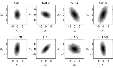
Figure 1: Contour plots for the tomogram in the phase space for the squeezed vacuum state with $\beta=4/5$ at different times. We used for the parametric amplifier $\Omega=9$, $k=2$, $\omega_{a}=1$, and $\omega_{b}=3$. The tomogram parameters are $\mu_{1}=\cos\pi/4,\nu_{1}=\sin\pi/4$, $\mu_{2}=\cos\pi/8,\nu_{2}=\sin\pi/8$.

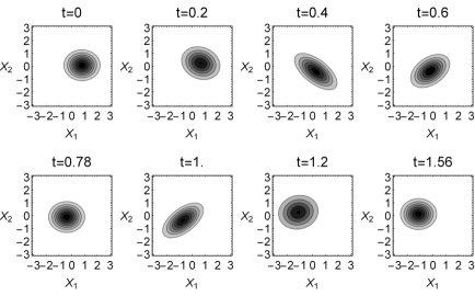
Figure 2: Contour plots for the tomogram in the phase space for the coherent state with $\alpha_{1}=4/5$, $\alpha_{2}=1/10$ at different times. The parameters of the parametric amplifier are the same as in Fig. 1 with the tomogram parameters are $\mu_{1}=\cos\pi/4,\nu_{1}=\sin\pi/4$ and $\mu_{2}=\cos\pi/8,\nu_{2}=\sin\pi/8$.

5 Discretization of the density matrix, von Neumann and linear entropies

The entanglement between two input modes in the parametric amplifier has been shown to exist through different methods, as second order correlations [49, 7] and the calculation of the Duan et al. criterion [50]. The entanglement between two modes in a symmetric Gaussian state have been described through EPR inequalities and the von Neumann entropy in [51]. The entanglement present in the parametric amplifier has been used in quantum metrology [52] and entanglement swapping [53]. Also the entanglement in other parametric processes, related to the amplification as the parametric oscillation is frequently used to generate correlated light [54, 55, 56] and implement quantum information protocols [57, 58]. The von Neumann and linear entropies are generally used to measure the entanglement between the modes of a bipartite pure system. However the analytic calculation of these quantities is, in general, not an easy matter. In this section, we provide a numerical method to calculate both entropies for a continuous variable density matrix using a discrete form. This method also can be used to define a positive map between the density matrix and other sub-matrices similar to the reduced density matrices that retain information on the entanglement of the system.

In order to compare the results and to evaluate the entanglement given by the tomographic representation discussed later, we calculate the von Neumann and linear entropies for the two-variable system.

The density matrix resulting from the time evolution of the Gaussian state described by Eq. (24) is a continuous function of the coordinates

$$\rho(x^{\prime}_{1},x^{\prime}_{2},x_{1},x_{2},t)=\langle x^{\prime}_{1},x^{\prime}_{2}|\rho(t)|x_{1},x_{2}\rangle=\psi^{*}(x^{\prime}_{1},x^{\prime}_{2},t)\,\psi(x_{1},x_{2},t)\ .$$ (65)

To determine the entanglement properties from a continuous variable density matrix, the discrete form of the density operator is made. Let us take four sets of discrete numbers along the axis that define the density matrix variables, that is,

$$\{x_{1_{1}}^{\prime},x_{1_{2}}^{\prime},\cdots,x_{1_{N}}^{\prime}\}\,,\>\{x_{2_{1}}^{\prime},x_{2_{2}}^{\prime},\cdots,x_{2_{N}}^{\prime}\}\,,\ \{x_{1_{1}},x_{1_{2}},\cdots,x_{1_{N}}\}\,,\ \{x_{2_{1}},x_{2_{2}},\cdots,x_{2_{N}}\}\,,$$

where the size of the steps is $\Delta x_{1}=x_{1_{r+1}}-x_{1_{r}}$ and $\Delta x_{2}=x_{2_{r+1}}-x_{2_{r}}$. One can notice that, to define properly the transpose matrix, one should take the same number of elements for the coordinates $x_{i}$ and $x^{\prime}_{i}$ and, for simplicity, let us choose the same step between them: $\Delta x_{1}^{\prime}=\Delta x_{1}$ and $\Delta x_{2}^{\prime}=\Delta x_{2}$. These partitions must be chosen to guarantee the normalization condition of the density matrix.

Therefore, the discrete two-mode density matrix can be expressed as

$$\rho_{i,j,k,l}(t)=\rho(x_{1_{i}}^{\prime},x_{2_{j}}^{\prime},x_{1_{k}},x_{2_{l}},t),$$

where the normalization condition is expressed in the form

$$\sum_{i,j=1}^{N}\rho_{i,j,i,j}(t)\Delta x_{1}\Delta x_{2}=1\ .$$

Then, the corresponding definition of the partial density matrix of the mode 1 is given by

$$\rho_{i,j}^{(1)}(t)=\sum_{k=1}^{N}\rho_{i,k,j,k}(t)\Delta x_{2}\ ,$$

obtaining the eigenvalues of the reduced density matrix provide us with a method to calculate either the linear or the von Neumann entropies.

The eigenvectors and eigenvalues are obtained by solving the standard eigenvalue equation for the matrix $\rho^{(1)}_{ij}(t)\Delta x_{1}$. Denoting the corresponding eigenvalues as $\{e_{k}(t)\}$, the linear and von Neumann entropies can be calculated as

$$S_{L}=1-\sum_{k=1}^{N}e_{k}^{2}(t),\qquad S_{VN}=-\sum_{k=1}^{N}e_{k}(t)\ln(e_{k}(t))\ .$$ (66)

For the squeezed vacuum state the linear entropy is given by

$$S_{L}(t)=\frac{2\left|\eta(t)\right|^{2}}{1+\left|\eta(t)\right|^{2}}\ ,$$ (67)

with $\eta$ given by Eq. (47). Similarly, for the von Neumann entropy, one gets

$$S_{VN}(t)=-\ln\left(1-\left|\eta(t)\right|^{2}\right)-\frac{\left|\eta(t)\right|^{2}\ln\left(\left|\eta(t)\right|^{2}\right)}{1-\left|\eta(t)\right|^{2}}\ .$$ (68)

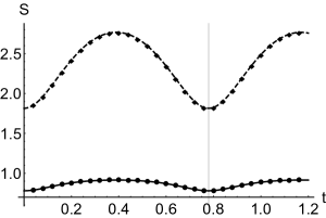
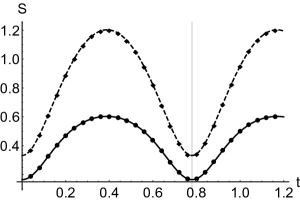
Figure 3: The analytic results for the linear entropy (solid black) and von Neumann entropy (dashed black) as functions of time for the squeezed vacuum state with the squeeze parameter (left) $\beta=4/5$ and (right) $\beta=3/10$. For the parametric amplifier, we take $\Omega=9$, $k=2$, $\omega_{a}=1$, and $\omega_{b}=3$. The corresponding numerical results are also shown in this figure where the linear entropy is indicated by a black dotted curve while the von Neumann entropy is displayed by a black rhombus curve.

In Fig. 3, we compare the analytic and numerical results for the von Neumann and linear entropies for a squeezed vacuum state evolving in the parametric amplifier. The difference between the analytic and numerical results has a maximum value of $10^{-6}$. In this figure, one can see that the same entanglement is obtained for times $t=0$ and $t=\pi/\nu$, as both entropies show a periodic behavior with period $T=\pi/\nu$.

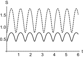
Figure 4: The linear entropy (solid curve) and von Neumann entropy (dashed curve) as functions of time for the coherent state with parameters $\alpha_{1}=1$, $\alpha_{2}=3$ (left) and for the particular Gaussian state with $a_{11}=1$, $a_{22}=3$, and $a_{12}=1.4$ (right). We use the same parameter values for the parametric amplifier as in Fig. 3.

Also in Fig 4, the von Neumann and linear entropies for the coherent state and a particular Gaussian state are presented. We have used the values $a_{11}=1$, $a_{22}=3$, $a_{12}=1.4$, $\Omega=9$, $k=2$, $\nu=\sqrt{\Omega^{2}/4-k^{2}}=\sqrt{65}/2$, $\omega_{a}=1$, and $\omega_{b}=3$. We can observe again an oscillatory behavior of period $T=\pi/\nu$. Also one can see that in the coherent state the two modes initially are not entangled but the evolution in the parametric amplifier makes these two modes entangled.

The oscillation of the entropies imply that there is entanglement between the two Gaussian modes even when initially are not entangled due to the evolution in the parametric amplifier. This entanglement has a maximum value at times $t=n\pi/(2\nu)$ for $n$ odd and has a minimum value at times $t=n\pi/\nu$ with $n$ even. We note that the minimum value for the entanglement is equal to the initial entropy, so given an initial entangled state the evolution in the amplifier can increase the entanglement between the modes.

6 Qubit portrait of symplectic tomograms

In this section, the qubit portrait of a symplectic tomogram is defined and calculated, in particular, for two-mode pure Gaussian states evolving in the parametric amplifier. This qubit portrait is the reduction of a symplectic or optical tomograms to a $4$ component probability vector, which for simply separable states is the tensor product of two-dimensional probability vectors.

This qubit portrait can be used to determine a Bell-type inequality where the violation of the parameter $|\mathcal{B}|\leq 2$ indicates that the bipartite system cannot be separable, i.e., it is entangled. Now, the converse statement is not true.

The spin tomograms for time-dependent Hamiltonians linear in spin variables have been constructed in [44]. These tomograms have been also used to study qubits and qudits within the quantum information context of separable and entangled states [45]. To define the qubit portrait for a continuous variable system, we generalize the idea developed for the spin tomogram, for which a qubit portrait of qudit states and Bell-type inequalities have been proposed in [24].

The spin states can be described by a probability distribution called spin tomogram denoted by $\omega(m,\vec{n})$, where $m$ is the projection in the direction $\vec{n}$ [43]. In general, the tomogram of a $d$-dimensional qudit system has $2^{d}$ components corresponding to the different projections of the angular momentum operator. The qubit portrait is defined as the reduction of the tomogram of a qudit system to a two-qubit tomogram. To construct the portrait, we reduce the $2^{d}$ components to only 4; to make this, we construct 4 arbitrary sets of this components and sum them.

In an analogous form, one can reduce all the information contained in the symplectic or optical tomograms to $4$ numbers related with the probabilities to find the quadrature components $X_{1}$ and $X_{2}$ into the $4$ integration regions ($\mathbb{A}_{1},\mathbb{A}_{2},\mathbb{A}_{3},\mathbb{A}_{4}$), that do not overlap $\mathbb{A}_{i}\cap\mathbb{A}_{j}=\emptyset$; and the union of all these regions is equal to the complete two-dimensional space $\mathbb{R}^{2}$. Then each components of the four-dimensional probability vector will be given by

$$P_{i}(\boldsymbol{\mu}_{1},\boldsymbol{\mu}_{2})=\int_{\mathbb{A}_{i}}\mathcal{W}(X_{1},X_{2},\mu_{1},\nu_{1},\mu_{2},\nu_{2};t)dX_{1}dX_{2},$$ (69)

with $i=1,\cdots,4$ and $\boldsymbol{\mu}_{k}=(\mu_{k},\nu_{k})$.

Then, we define a $4\times 4$ stochastic matrix $\mathbf{M}$ as follows:

$$\mathbf{M}=\left(\begin{array}[]{cccc}P_{1}(\boldsymbol{\mu}_{a},\boldsymbol{\mu}_{b})&P_{1}(\boldsymbol{\mu}_{a},\boldsymbol{\mu}_{c})&P_{1}(\boldsymbol{\mu}_{d},\boldsymbol{\mu}_{b})&P_{1}(\boldsymbol{\mu}_{d},\boldsymbol{\mu}_{c})\\ P_{2}(\boldsymbol{\mu}_{a},\boldsymbol{\mu}_{b})&P_{2}(\boldsymbol{\mu}_{a},\boldsymbol{\mu}_{c})&P_{2}(\boldsymbol{\mu}_{d},\boldsymbol{\mu}_{b})&P_{2}(\boldsymbol{\mu}_{d},\boldsymbol{\mu}_{c})\\ P_{3}(\boldsymbol{\mu}_{a},\boldsymbol{\mu}_{b})&P_{3}(\boldsymbol{\mu}_{a},\boldsymbol{\mu}_{c})&P_{3}(\boldsymbol{\mu}_{d},\boldsymbol{\mu}_{b})&P_{3}(\boldsymbol{\mu}_{d},\boldsymbol{\mu}_{c})\\ P_{4}(\boldsymbol{\mu}_{a},\boldsymbol{\mu}_{b})&P_{4}(\boldsymbol{\mu}_{a},\boldsymbol{\mu}_{c})&P_{4}(\boldsymbol{\mu}_{d},\boldsymbol{\mu}_{b})&P_{4}(\boldsymbol{\mu}_{d},\boldsymbol{\mu}_{c})\end{array}\right).$$ (70)

Here, each column vector specify the two-dimensional coordinate system where the measurements of the position operators are realized. Each one of them satisfy $\sum_{k}P_{k}(\boldsymbol{\mu}_{l},\boldsymbol{\mu}_{k})=1$. It can be shown that in the case of a simply separable state, the matrix $\mathbf{M}$ can be written as the direct product of two subsystems. In this case, one can define a Bell-type inequality.

Let us consider two stochastic matrices $\left(\begin{array}[]{cc}x&y\\ 1-x&1-y\end{array}\right)$,$\quad\left(\begin{array}[]{cc}t&z\\ 1-t&1-z\end{array}\right)$, and their tensor product

$$\widetilde{\mathbf{M}}=\left(\begin{array}[]{cc}x&y\\ 1-x&1-y\end{array}\right)\otimes\left(\begin{array}[]{cc}t&z\\ 1-t&1-z\end{array}\right)\,.$$ (71)

It is straightforward to show that the matrix elements of $\widetilde{M}_{jk}(x,y,z,t)$ satisfy the Laplace equation

$$\left(\frac{\partial^{2}}{\partial x^{2}}+\frac{\partial^{2}}{\partial y^{2}}+\frac{\partial^{2}}{\partial z^{2}}+\frac{\partial^{2}}{\partial t^{2}}\right)\widetilde{M}_{jk}(x,y,z,t)=0\,.$$

This means that the extreme values of any function

$$\mathcal{B}(x,y,z,t)=\sum_{j,k=1}^{4}\widetilde{M}_{jk}(x,y,z,t)\,{C}_{kj}$$ (72)

are situated on the boundaries of the region where $x,y,z,t$ are given. In our case, it is the cube $0\leq x,y,z,t\leq 1$. For this work we have taken the coefficient $C_{kj}$ in the matrix form

$$\mathbf{C}=\left(\begin{array}[]{cccc}1&-1&-1&1\\ 1&-1&-1&1\\ 1&-1&-1&1\\ -1&1&1&-1\end{array}\right),$$

although the election of $\mathbf{C}$ is not unique, this matrix had been chosen in order to obtain a function $\mathcal{B}$ with two elements from each column of $\widetilde{\mathbf{M}}$ with a positive sign and two elements with negative sign. In the case where all this elements cancel each other the parameter $\mathcal{B}$ would be equal to zero and in general one can check that the following inequality holds:

$$|\mathcal{B}(x,y,z,t)|\leq 2\ .$$ (73)

Using the stochastic matrix $\mathbf{M}$, as in Eq. (71), and taking the definition of the Bell-type parameter, as in Eq. (72), one can evaluate the inequality

$$|\mathcal{B}|=|E(a,b)+E(a,c)+E(d,b)-E(d,c)|\leq 2$$ (74)

where $E(x,y)=P_{1}(\boldsymbol{\mu}_{x},\boldsymbol{\mu}_{y})-P_{2}(\boldsymbol{\mu}_{x},\boldsymbol{\mu}_{y})-P_{3}(\boldsymbol{\mu}_{x},\boldsymbol{\mu}_{y})+P_{4}(\boldsymbol{\mu}_{x},\boldsymbol{\mu}_{y})$. This inequality evaluates, if the matrix $\mathbf{M}$ can be expressed as a direct product of two subsystems, all the separable states must satisfy this condition. Therefore, a violation of this inequality is a sufficient condition for entanglement.

To establish properly the Bell-type inequality, the integrating regions used in the construction of the matrix $\mathbf{M}$ should be taken as the direct product of the two regions in $X_{1}$ and $X_{2}$ in order to preserve the product structure of the matrix $\mathbf{M}$, this is,

$$\left(\begin{array}[]{c}\mathbb{A}_{1}\\ \mathbb{A}_{2}\\ \mathbb{A}_{3}\\ \mathbb{A}_{4}\end{array}\right)=\left(\begin{array}[]{c}\mathcal{L}_{1}^{(1)}\\ \mathcal{L}_{2}^{(1)}\end{array}\right)\otimes\left(\begin{array}[]{c}\mathcal{L}_{1}^{(2)}\\ \mathcal{L}_{2}^{(2)}\end{array}\right)\ ,$$ (75)

where $\sum^{4}_{k=1}{\mathbb{A}_{k}}=\mathbb{R}^{2}$ and $\sum_{i=1}^{2}\mathcal{L}_{i}^{(j)}=(-\infty,\infty)$, with $j=1,2$. We enhance that the probabilities necessary to the definition of $\widetilde{\mathbf{M}}$ in Eq. (70) can be obtained making use of a discrete scheme for the tomogram, similar to the one used for the density matrix in Section 5. In that scheme the probabilities are the discrete integral over the different areas $\mathbb{A}_{1}$ to $\mathbb{A}_{4}$. Using this discrete form and the fact that the optical tomogram can be observed experimentally [59] provide the possibility to measure this probabilities and to make measurements of the Bell inequalities previously studied.

In the present work, we consider

$$\mathcal{L}_{1}^{(j)}=(-\infty,0],\quad\mathcal{L}_{2}^{(j)}=[0,\infty),\quad\textrm{with }j=1,2\ ,$$ (76)

these areas and line elements are represented in Fig. 5.

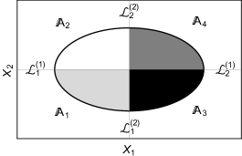
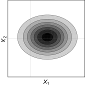
Figure 5: (Left) Different regions $\mathbb{A}_{1}$ to $\mathbb{A}_{4}$ taken to define the probabilities in matrix $\mathbf{M}$, i.e. for a fixed $(\boldsymbol{\mu}_{1},\boldsymbol{\mu}_{2})$. The ellipse represents a contour plot of the tomogram and in the different colors are the areas corresponding to each of the four components in a column of $\mathbf{M}$. To compute the parameter $\mathcal{B}$ one need to obtain the corresponding areas for the other three values of $(\boldsymbol{\mu}_{1},\boldsymbol{\mu}_{2})$. (Right) Contour plot of the symplectic tomogram displaying the four different regions for a coherent state

For the coordinate axes where the tomogram are measured, we used two different sets of parameters indicated in Table 1.

$\boldsymbol{\mu}=(\mu,\nu)$	$\theta$	$\boldsymbol{\mu}=(\mu,\nu)$	$\theta$
${\boldsymbol{\mu}_{a}=(-0.39,\ -0.92})$	$4.31\ (246.9^{\circ})$	${\boldsymbol{\mu}_{a}=(\quad 1,\ 0})$	0
${\boldsymbol{\mu}_{b}=(-0.99,\ -0.01})$	$3.15\ (180.5^{\circ})$	${\boldsymbol{\mu}_{b}=(0.92,\ 0.38})$	$\pi/8$
${\boldsymbol{\mu}_{c}=(\ \ 0.02,\ \ \ 0.99})$	$1.54\ (88.2^{\circ})$	${\boldsymbol{\mu}_{c}=(0.38,\ 0.92})$	$3\pi/8$
${\boldsymbol{\mu}_{d}=(-0.60,\ -0.80})$	$4.07\ (233.2^{\circ})$	${\boldsymbol{\mu}_{d}=(1/\sqrt{2},\ 1/\sqrt{2}})$	$\pi/4$

Table 1: The parameters are given by $(\mu,\nu)=(s\cos\theta,s^{-1}\sin\theta)$ with $s=1$. The angles and scaling factors taking in the qubit portrait are indicated, the selected values satisfy the constraint $2|\mu\nu|\leq 1$.

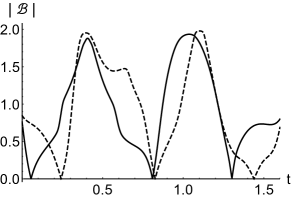
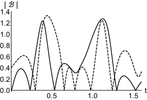
Figure 6: Plot of the parameter $|\mathcal{B}|$ as a function of time for the squeezed vacuum state with squeezing parameter $\beta=4/5$ (left) and for the coherent state with parameters $\alpha_{1}=4/5$ and $\alpha_{2}=1/10$ (right). Here, the amplifier parameters are: $\omega_{a}=1$, $\omega_{b}=3$, $\Omega=9$, $k=2$, and $\nu=\sqrt{65}/2$. In both cases, the solid black curve corresponds to a system, where the parameters $\boldsymbol{\mu}$ are given at the left of Table  1, and for the dashed curve, the parameters are given at the right of Table 1.

In Fig. 6, the evaluation of the parameter $\mathcal{B}$ is given for the squeezed vacuum state and the coherent state, respectively. We did not found a violation of the bound 2 for the parameter $\mathcal{B}$ in the two cases, although the analysis was made for several partitions. It can be seen for the non-continuous curve at times around $t=0.3$ and $t=1$ that the $\mathcal{B}$ parameter for the squeezed vacuum state is almost zero. At these times, the contour plot of the tomogram of Fig. 1 exhibits a small variance in one of the principal axis of symmetry. In contrast to the times where the Bell parameter $\mathcal{B}$ is near the value 2 (times around $0.5$ and $1.2$), the tomogram displays a more symmetric distribution.

For the coherent state, the Bell parameter shows faster oscillations than for the squeezed vacuum state and the local maxima are smaller. This can be related to the displacement of the tomogram (see Fig. 2), which implies also to the fact that the variance, the mean values, and the probabilities defining the matrix $\mathbf{M}$ are changing in a more complicated form.

6.1 Alternative method

Here, we want to propose an alternative form of using the portrait tomogram of the Bell’s parameter, which uses the fact that the tomogram of a non-entangled two-dimensional state can be put as the product of the reduced tomograms, as in Eq. (59). The difference of the probabilities $\int_{\mathbb{A}}\mathcal{W}(1,2)dX_{1}dX_{2}-\int_{\mathcal{L}^{(1)}}\mathcal{W}(1)dX_{1}\int_{\mathcal{L}^{(2)}}\mathcal{W}(2)dX_{2}$ is zero when the system state is simply separable. This implies that the matrix $\widetilde{\mathbf{M}}$ of the product of the reduced tomograms $\mathcal{W}(1)\mathcal{W}(2)$ must be equal to the complete two-variable tomogram $\mathcal{W}(1,2)$. Defining the matrix $\widetilde{\mathbf{M}}$ of the product of the reduced tomograms as in Eq. (71) where the probabilities are defined as

$$x=\int_{\mathcal{L}^{(1)}_{1}}\mathcal{W}_{1}(X_{1},\mu_{a},\nu_{a})\ dX_{1},\quad y=\int_{\mathcal{L}^{(1)}_{1}}\mathcal{W}_{1}(X_{1},\mu_{d},\nu_{d})\ dX_{1},$$

$$t=\int_{\mathcal{L}^{(2)}_{1}}\mathcal{W}_{2}(X_{2},\mu_{b},\nu_{b})\ dX_{2},\quad z=\int_{\mathcal{L}^{(2)}_{1}}\mathcal{W}_{2}(X_{2},\mu_{c},\nu_{c})\ dX_{2},$$ (77)

then a parameter $\widetilde{\mathcal{B}}$ corresponding to this matrix $\widetilde{\mathbf{M}}$ can be defined in the form

$$\widetilde{\mathcal{B}}=\sum_{j,k=1}^{4}\widetilde{M}_{jk}C_{kj}\ .$$ (78)

For non-entangled pure states, the subtraction of the parameter for the complete tomogram $\mathcal{B}$ and the product of the reduced tomograms $\widetilde{\mathcal{B}}$ must satisfy the equality

$$|\mathcal{B}-\widetilde{\mathcal{B}}|=0\ ,$$ (79)

while the entangled states satisfy the inequality

$$|\mathcal{B}-\widetilde{\mathcal{B}}|>0\ .$$ (80)

The condition (80) can be used to distinguish entangled from non-entangled states but the converse statement is not always fulfilled, i.e., the condition $|\mathcal{B}-\widetilde{\mathcal{B}}|=0$ does not imply that the system state is separable. Therefore, the expression in Eq. (79) is a necessary condition for the system state to be separable and a violation to this equality is a sufficient condition for entanglement.

The quantity $\widetilde{\mathcal{B}}$ can be measured experimentally in the discrete scheme of the tomogram, making possible the evaluation of the separability criteria $|\mathcal{B}-\widetilde{\mathcal{B}}|$ for these systems.

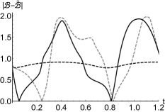
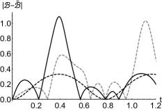
Figure 7: The parameter $|\mathcal{B}-\widetilde{\mathcal{B}}|$ and the linear entropy $S_{L}$ (black dashed) as functions of time for the squeezed vacuum state with squeezing parameter $\beta=4/5$ (left) and for the coherent state with parameters $\alpha_{1}=4/5$ and $\alpha_{2}=1/10$ (right); the amplifier parameters are: $\omega_{a}=1$, $\omega_{b}=3$, $\Omega=9$, $k=2$, and $\nu=\sqrt{65}/2$. In both cases, the solid black curve corresponds to a system where the parameters $\boldsymbol{\mu}$ are given at the left of Table 1 and for the gray dashed curve the parameters are given at the right of Table 1.

In Fig. 7, the plots for $|\mathcal{B}-\widetilde{\mathcal{B}}|$ are shown for the evolution of the squeezed vacuum state and for the coherent state as functions of time. It can be seen that for times equal to multiples of the frequency $\pi/\nu$ the coherent states are separable as indicated by the von Neumann and linear entropies and the system state is separable for those time for the squeezed vacuum state. One can point out that for some times the parameter $|\mathcal{B}-\widetilde{\mathcal{B}}|$ tends to zero even when the system is entangled (as seen in the linear and von Neumann entropies); this behavior is present because the condition in Eq. (79) is not a sufficient condition to guarantee separability.

6.2 No-signaling correlations

Following the ideas of Popescu and Rohrlich that the relativistic causality does not constraint the CHSH correlations to the Cirelson bound, we are going to study the correlations of the reduced tomogram

$$\mathcal{W}_{1}(X_{1},\mu_{1},\nu_{1};t)=\int\mathcal{W}(X_{1},\mu_{1},\nu_{1};X_{2},\mu_{2},\nu_{2};t)dX_{2}\,,$$

without taking expression (75) into account. This can be done by constructing the $4\times 4$ stochastic matrix $\mathbf{M}$ as follows:

$$\mathbf{M}=\left(\begin{array}[]{cccc}P_{1}(\mu_{a},\nu_{b})&P_{1}(\mu_{a},\nu_{c})&P_{1}(\mu_{d},\nu_{b})&P_{1}(\mu_{d},\nu_{c})\\ P_{2}(\mu_{a},\nu_{b})&P_{2}(\mu_{a},\nu_{c})&P_{2}(\mu_{d},\nu_{b})&P_{2}(\mu_{d},\nu_{c})\\ P_{3}(\mu_{a},\nu_{b})&P_{3}(\mu_{a},\nu_{c})&P_{3}(\mu_{d},\nu_{b})&P_{3}(\mu_{d},\nu_{c})\\ P_{4}(\mu_{a},\nu_{b})&P_{4}(\mu_{a},\nu_{c})&P_{4}(\mu_{d},\nu_{b})&P_{4}(\mu_{d},\nu_{c})\end{array}\right),$$ (81)

which satisfy the normalization condition $\sum_{k}P_{k}(\mu_{a},\nu_{b})=1$ for all column vectors and the probabilities given by

$$P_{i}(\mu,\nu)=\int_{\mathcal{L}_{i}}\mathcal{W}_{1}(X_{1},\mu,\nu;t)dX_{1}\ ,$$ (82)

where $\mathcal{L}_{i}$ defines the integration region. One has that $\sum^{4}_{k=1}{\mathcal{L}_{k}}=(-\infty,\infty)$ are the different regions of the $X_{1}$ space where the normalization condition holds.

The different $\mu$, $\nu$ parameters taken to establish the matrix $\mathbf{M}$ of the reduced symplectic tomogram are listed in Table 2. In Fig. 8, the corresponding measurement angles $\theta$ used to establish the stochastic matrix $\mathbf{M}$ are shown. Notice that the integration variable in each case $X_{1}$ is also scaled.

One can construct the Bell parameter by multiplying the matrix $\mathbf{M}$ with $\mathbf{C}$, but now its value is only constrained in the interval $0\leq|\mathcal{B}|\leq 4$. Then, these correlations are not of the Bell type, given that the partition used to construct the matrix $\mathbf{M}$ tomogram is not of the form of a direct product of two subsystems. For that reason, the Cirelson bound $2\sqrt{2}$ is also violated for the parameter $\mathcal{B}$,

($\mu,\nu$)	$\theta$ (rad)	$s$
($\mu_{a}=0.1,\ \nu_{b}=0.2$)	0.02 (1.15∘)	0.1
($\mu_{a}=0.1,\ \nu_{c}=0.3$)	0.03 (1.72∘)	0.1
($\mu_{d}=0.4,\ \nu_{b}=0.2$)	0.08 (4.58∘)	0.4
($\mu_{d}=0.4,\ \nu_{c}=0.3$)	0.12 (6.87∘)	0.4

Table 2: The parameters are given by $(\mu,\nu)=(s\cos\theta,s^{-1}\sin\theta)$. The angles and scaling factors taking in the qubit portrait are indicated, the selected values satisfy the constraint $2|\mu\nu|\leq 1$.

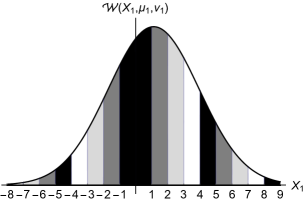
Figure 8: (left) Partition used to make the portrait tomogram for the different initial states. The region I ($\mathcal{L}_{1}$) is taken from 0 to $\pm$1, $\pm$4 to $\pm$5, $\pm$8 to $\pm$9, $\cdots$ here denoted by the black area under the reduced tomogram. The second region ($\mathcal{L}_{2}$) is taken from $\pm$1 to $\pm$2, $\pm$5 to $\pm$6, $\pm$9 to $\pm$10, $\cdots$, displayed in dark gray color. For the region III ($\mathcal{L}_{3}$), we have $\pm$2 to $\pm$3, $\pm$6 to $\pm$7, $\pm$10 to $\pm$11, $\cdots$, in light gray. The last region ($\mathcal{L}_{4}$) is taken $\pm$3 to $\pm$4, $\pm$7 to $\pm$8, $\pm$11 to $\pm$12, $\cdots$, which is the white region under the tomogram. (Right) Plots of the different $\theta$ angles defined by the parameters $\mu$, $\nu$ in Table 2. Notice that along these lines the tomogram is integrated in the regions mentioned before.

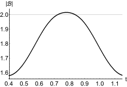
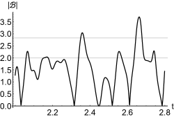
Figure 9: Parameter $\mathcal{B}$ as function of time. (Left) for the squeezed vacuum state with $\beta=4/5$ and (right) for the coherent state with $\alpha_{1}=100$, $\alpha_{2}=3$, the parameters of the parametric amplifier were $\Omega=1/40$, $k=1/10$, $\omega_{a}=1$, and $\omega_{b}=3$.

It can be seen in Fig. 9 that there is a strong correlation in the artificial partition of the reduced tomogram.

The behavior of the parameter $|\mathcal{B}|$ in the constructed stochastic matrix $M$ completely corresponds to the Rohrlich–Popescu result [21]. In our case, we obtained the result that the qubit portrait of the one mode of the amplifier state tomogram is completely different from the qubit-portrait behavior of the qudit-system state.

7 Conclusions

We constructed the linear time-dependent invariants for the non-degenerated parametric amplifier for the trigonometric and hyperbolic cases. These invariants are used to determine in analytic form the evolution of two-mode Gaussian wave packets, which is always a Gaussian state characterized by the covariance matrix in (24) and (36). Also we noted that the evolution of a squeezed vacuum state is also a squeezed vacuum state.

The corresponding tomographic representation of the states was calculated in (62) and (64) and plotted in the phase space $X_{1}-X_{2}$ displaying clearly the presence of the squeezing phenomena.

To calculate the entanglement between the idler and signal modes of the parametric amplifier, we establish a discretization of the density matrix which, in principle, leads to an infinite matrix full of zeros plus a finite $N\times N$ density matrix. By means of this finite matrix, we have calculated the linear and von Neumann entropies. For the evolution of the vacuum state, we have analytic results for the entropies in Eqs. (67) and (68), which are compared with the results of the discretization for two different values of the squeezing parameter $\beta$, the mean square deviation is of the order of $10^{-6}$. The corresponding calculations for the coherent and Gaussian states are also determined by the discretization procedure. In all the cases, we have a periodic behavior (with period $T=\pi/\nu$). If we want to determine the results for the hyperbolic case of the parametric amplifier, we can do an analytic continuation in the parameters of the model. We point out that the periodic nature of the entropies is present even when the state is not periodic. We also have shown that the initial entanglement can be amplified due to the evolution in the parametric amplifier, the maxima values occur at times $t=(2n+1)\,\pi/(2\nu)$ while the minima values occur at time equal to zero and $t=2n\,\pi/\nu$, $n\in\mathbb{Z}$.

In this work, we establish another procedure to determine the entanglement of the system, which is based on a qubit portrait of a symplectic (or optical) tomogram. This portrait uses the properties of the stochastic matrices to define a Bell-type parameter $\mathcal{B}$, which must satisfy the inequality $\mathcal{B}\leq 2$. The method reduces the continuous probability of the tomogram to a $4\times 4$ stochastic matrix which must satisfy the previous inequality, if it can be written as a direct product of two stochastic matrices. This must be done by taking into account carefully the integration regions of the continuous variables $X_{1}$ and $X_{2}$. We have selected several possible partitions to have a violation of the Bell-type inequality without success.

For a composite system, the integral for joint probability $\int_{\mathbb{A}}\mathcal{W}(1,2)\,dX_{1}\,dX_{2}$ is equal to the product $\int_{\mathcal{L}^{(1)}}\mathcal{W}(1)\,dX_{1}\int_{\mathcal{L}^{(2)}}\mathcal{W}(2)\,dX_{2}$. Then, one can say that there are no correlations between the measurements of the probabilities in the two-variable system and its state is simply separable. Therefore, one can assume that it is simply separable and define the Bell-type parameter $\widetilde{\mathcal{B}}$ for the factorized tomogram, which leads to establish the equality $|\mathcal{B}-\widetilde{\mathcal{B}}|=0$. This equality is a necessary condition for the system to be separable and a violation of this condition is a sufficient condition to determine the entanglement.

We study also the behavior of another type of correlations by constructing a $4\times 4$ stochastic matrix without taking into account that the different integration regions can be written as a direct product of two subsystems.

As it is shown in Fig. 9, when the matrix $\mathbf{M}$ is multiplied by $\mathbf{C}$ and a new parameter $\mathcal{B}$ is defined, one can see that this pàrameter can take values larger than the Cirelson bound.

Finally, we want to enhance that the discretization procedure of the density matrix can be expressed as a nonlinear positive mapping to reduce even further the $N\times N$ density matrix without losing information on the entanglement of the system as, for example, if it has a large quantity of zeros. This method is currently explored and it will be presented in a future publication.

Appendix A Linear time-dependent invariants

The time-dependent invariants are operators $\Gamma$ that satisfy

$$\frac{d\Gamma}{dt}=0=\frac{1}{i\hbar}[\Gamma,H]+\frac{\partial\Gamma}{\partial t}\ .$$ (83)

For quadratic Hamiltonians, $\Gamma$ is linear in the annihilation and creation operators [2]. Therefore, for the parametric amplifier, one proposes an invariant of the form

$$\Gamma=\gamma_{1}a+\gamma_{2}b+\gamma_{3}a^{\dagger}+\gamma_{4}b^{\dagger}\,,$$

which being substituted into Eq. (83) yields a coupled pair of differential equations

$$\dot{\gamma}_{1}-i\gamma_{1}\omega_{a}-ik\gamma_{4}e^{i\omega t}=0\,,\quad\dot{\gamma}_{4}+i\gamma_{4}\omega_{b}+ik\gamma_{1}e^{-i\omega t}=0\,,$$

$$\dot{\gamma}_{2}-i\gamma_{2}\omega_{b}-ik\gamma_{3}e^{i\omega t}=0\,,\quad\dot{\gamma}_{3}+i\gamma_{3}\omega_{a}+ik\gamma_{2}e^{-i\omega t}=0\,.$$

To solve these sets of coupled differential equations, we consider the transforms $\gamma_{1}=e^{i\omega_{a}t}g_{1}$ and $\gamma_{4}=e^{-i\omega_{b}t}g_{4}$ together with $\gamma_{2}=e^{i\omega_{b}t}g_{2}$ and $\gamma_{3}=e^{-i\omega_{a}t}g_{3}$. Substituting these expressions into Eq. (A), one arrives at

$$\dot{g}_{1}=ike^{i\Omega t}g_{4},\qquad\dot{g}_{4}=-ike^{-i\Omega t}g_{1},$$ (84)

where $\Omega=\omega-\omega_{a}-\omega_{b}$; and then

$$\ddot{g}_{1}-i\Omega\dot{g}_{1}-k^{2}g_{1}=0$$

whose solution, for the initial conditions $g_{1}(0)=1$, $g_{4}(0)=0$, is

$$g_{1}(t)=e^{i\Omega/2t}\left(\cos\nu t-\frac{i\Omega}{2\nu}\sin\nu t\right)\ ,$$

$$g_{4}(t)=-\frac{ik}{\nu}e^{-i\Omega t}\sin\nu t\ .$$ (85)

with $\nu=\sqrt{\Omega^{2}/4-k^{2}}$.

Noticing that $g_{2}$ and $g_{3}$ must satisfy the same differential equations that $g_{1}$ and $g_{4}$, respectively, but now for the initial conditions $g_{2}(0)=0$ and $g_{3}(0)=0$, one gets $g_{2}(t)=g_{3}(t)=0$.

If we now consider the initial conditions $g_{1}(0)=0$, $g_{2}(0)=1$, $g_{3}(0)=0$, $g_{4}(0)=0$, one has the same differential equations making the substitutions

$$g_{2}(t)\rightarrow g_{1}(t),\qquad g_{3}(t)\rightarrow g_{4}(t)$$

into Eq. (84).

Substituting properly the previous results, one arrives at expression (2) for the linear time-dependent invariants of the parametric amplifier. The quadrature operators for the two modes are defined as $P_{1}=i(A^{\dagger}-A)/\sqrt{2}$, $P_{2}=i\sqrt{\frac{\omega_{b}}{2}}(B^{\dagger}-B)$, $Q_{1}=(A+A^{\dagger})/\sqrt{2}$, and $Q_{2}=\frac{1}{\sqrt{2\omega_{b}}}(B+B^{\dagger})$, which can be written explicitly using Eq. (13).

References

- [1] I. A. Malkin, V. I. Man’ko, and D. A. Trifonov, Phys. Rev. D 2 1371 (1970).
- [2] V. V. Dodonov and V. I. Man’ko, Invariants and the evolution of nonstationary quantum systems, Proceedings of the Lebedev Physical Institute, vol. 183, (Nova Science Publishers, New York, 1989).
- [3] V. V. Dodonov and V. I. Man’ko, (Eds.), Theory of Nonclassical States of Light (Taylor-Francis, London, 2003).
- [4] S. K. Suslov, Phys. Scr. 81 055006 (2010).
- [5] O. Castaños, R. López-Peña, and V. I. Man’ko, J. Phys. A: Math. Gen. 27 1751 (1994).
- [6] R. P. Feynman, A. R. Hibbs and D. F. Styer, Quantum Mechanics and Path Integrals (Dover publications, New York, 2010).
- [7] P. K. Rekdal and B. K. Skagerstam, Phys. Scr. 61 296 (2000).
- [8] D. F. Walls and G. J. Milburn, Quantum Optics (Springer, Berlin, 1995).
- [9] K. Takashima, N. Hatakenaka, S. Kurihara, and A. Zeilinger, J. Phys. A: Math. Theor. 41 164036 (2008).
- [10] K. Takashima, S. Matsuo, T. Fujii, N. Hatakenaka, S. Kuri- hara, and A. Zeilinger, J. Phys.: Conf. Ser. 150 052260 (2009).
- [11] T. Fujii, S. Matsuo, N. Hatakenaka, S. Kurihara, and A. Zeilinger, Phys. Rev. B 84 174521 (2011).
- [12] S. Mancini, V. I. Man’ko, and P. Tombesi, Phys. Lett. A 213 1 (1996).
- [13] A. Einstein, B. Podolsky, N. Rosen, Phys. Rev. 47 777 (1935).
- [14] E. Schrödinger, Naturwiss. 23 807; 823; 844 (1935).
- [15] J. S. Bell, Physics 1 195 (1964).
- [16] J. F. Clauser, M. A. Horne, A. Shimony, and R. A. Holt, Phys. Rev. Lett. 23 880 (1969).
- [17] N. Brunner, D. Cavalcanti, S. Pironio, V. Scarani, S. Wehner, Rev. Mod. Phys. 86 419 (2014).
- [18] A. Aspect, P. Grangier, and G. Roger, Phys. Rev. Lett. 47 460 (1981).
- [19] O. Gühne, G. Tóth, Phys. Reports 474 1 (2009).
- [20] B. S. Cirelson, Lett. Math. Phys. 4 93 (1980).
- [21] S. Popescu and D. Rohrlich, Found. Phys. 24 379 (1994).
- [22] K. Banaszek and K. Wodkiewicz, Phys. Rev. Lett. 82 2009 (1999).
- [23] M. D’Angelo, A. Zavatta, V. Parigi, and M. Bellini, Phys. Rev. A 74 052114 (2006).
- [24] V. N. Chernega and V. I. Man’ko, J. Russ. Laser Res. 28 103 (2007).
- [25] M. A. Nielsen, and I. L. Chuang, Quantum Computation and Quantum Information (Cambridge University Press, London, 2010).
- [26] A. Ibort, V. I. Man’ko, G. Marmo , A. Simoni, and F. Ventriglia, Phys. Scr. 79 065013 (2009).
- [27] S. N. Fillipov, and V. I. Man’ko, J. Russ. Laser Res. 30 55 (2009).
- [28] W. H. Louisell, A Yariv, and A. E. Siegman, Phys. Rev. 124 1646 (1961).
- [29] B. R. Mollow and R. J. Glauber, Phys. Rev. 160 1076 (1967).
- [30] B. R. Mollow and R. J. Glauber, Phys. Rev. 160 1097 (1967).
- [31] M. E. Marhic, Fiber optical parametric amplifiers and related devices, (Cambridge University Press, London, 2007).
- [32] M. Jamshidifar, A. Vedadi and M. E. Marhic, 2014 “Continuous-Wave Two-pump Fiber Optical Parametric Amplifier with 60 dB Gain”, in CLEO: 2014, OSA Technical Digest (online) (Optical Society of America, 2014), paper JW2A.21.
- [33] A. Isar, Open Sys. Inf. Dynamics, 18 175 (2011).
- [34] A. Isar, Phys. Scr. T160 014019 (2014).
- [35] O. Castaños, R. López-Peña and V. I. Man’ko, J. Russ. Laser Res. 16 477 (1995).
- [36] O. Castaños, and J. López, Phys. Conf. Ser. 380 012017 (2012).
- [37] S. Spälter, N. Korolkova, F. König, A. Sizmann, and G. Leuchs, Phys. Rev. Lett. 81 786 (1998).
- [38] V. Boyer, A. M. Marino, R. C. Pooser, and P. D. Lett, Science 321 544 (2008).
- [39] F. A. S. Barbosa, A. S. Coelho, K. N. Cassemiro, P. Nussenzveig, C. Fabre, M. Martinelli, and A. S. Villar, Phys. Rev. Lett. 111 200402 (2013).
- [40] J. A. Levenson, I. Abram, Th. Rivera, and Ph. Grangier, J. Opt. Soc. Am. B 10 2233 (1993).
- [41] J. Wei, and E. Norman, J. Math. Phys. 4 575 (1963).
- [42] K. Vogel and H. Risken, Phys. Rev A 40 2847 (1989).
- [43] V. V. Dodonov and V. I. Man’ko, Phys. Lett. A 239 335 (1997).
- [44] O. Castaños, R. López-Peña, M. Man’ko, and V. I. Man’ko, J. Opt. B: Quantum Semiclass. Opt. 5 227 (2003).
- [45] V. I. Man’ko, G. Marmo, E. C. G. Sudarshan, and F. Zaccaria, Phys. Lett. A 327 353 (2004).
- [46] A. O. Niskanen, K. Harrabi, F. Yoshihara, Y. Nakamura, S. Lloyd, and J. S. Tsai, Science 316 723 (2007).
- [47] R. C. Bialczak, M. Ansmann, M. Hofheinz, M. Lenander, E. Lucero, M. Neeley, A. D. O’Connell, D. Sank, H. Wang, M. Weides, J. Wenner, T. Yamamoto, A. N. Cleland, and J. M. Martinis, Phys. Rev. Lett. 106 060501 (2011).
- [48] M. Ansmann, H. Wang, R. C. Bialczak, M. Hofheinz, E. Lucero, M. Neeley, A. D. O’Connell, D. Sank, M. Weides, J. Wenner, A. N. Cleland, and J. M. Martinis, Nature Lett. 461 504 (2009).
- [49] P. D. Drummond and M. D. Reid, Phys. Rev. A 41 3930 (1990).
- [50] Y. Fang and J. Jing, New J. Phys. 17 023027 (2015).
- [51] G. Giedke, M. M. Wolf, O. Krüger, R. F. Werner and J. I. Cirac, Phys. Rev. Lett. 91 107901 (2003).
- [52] F. Hudelist, J. Kong, C. Liu, J. Jing, Z.Y. Ou and W. Zhang, Nature Comm. 5 3049 (2014).
- [53] J. Zhang, C. Xie and K. Peng, Phys. Lett. A, 299 427 (2002).
- [54] M. D. Reid and P. D. Drummond, Phys. Rev. Lett. 60 , 2731 (1988).
- [55] K. N. Cassemiro, A. S. Villar, P. Valente, M. Martinelli and P. Nussenzveig, J. of Phys.: Conf. Ser. 84 012003 (2007).
- [56] A. S. Villar, K. N. Cassemiro, K. Dechoum, A. Z. Khoury, M. Martinelli and P. Nussenzveig, J. Opt. Soc. Am. B 24 249 (2007).
- [57] J. Jing, J. Zhang, Y. Yan, F. Zhao, C. Xie and K. Peng, Phys. Rev. Lett. 90 167903 (2003).
- [58] N. Takei, H. Yonezawa, T. Aoki and A. Furusawa, Phys. Rev. Lett. 94 220502 (2005).
- [59] M. Bellini, A. S. Coelho, S. N. Filippov, V. I. Man’ko and A. Zavatta, Phys. Rev. A 85 052129 (2012).