Stability of Axisymmetric Liquid Bridges

Abstract

We study stability of axisymmetric liquid bridges between two axisymmetric solid bodies in the absence of gravity under arbitrary asymmetric perturbations which are expanded into a set of angular Fourier modes. We determine the stability region boundary for every angular mode in case of both fixed and free contact lines. Application of this approach allows us to demonstrate existence of stable convex nodoid menisci between two spheres.

1 Introduction

An interface between two adjacent fluids both contacting solid(s) is called a capillary surface, which shape depends on liquid volumes and boundary conditions (BC) specified at the contact line where the liquids touch the solids. A liquid bridge (LB) emerges when a small amount of fluid (interfacing a surrounding liquid with different properties) contacts two (or more) solid bodies. The LB problem has long history in both theoretical physics and pure mathematics where the research mostly focused on two topics – menisci shapes and related parameters (volume $V$, surface area $A$ and surface curvature $H$) and menisci stability.

A menisci shape study was pioneered by Delaunay [4] who classified all surfaces of revolution with constant mean curvature satisfying the Young-Laplace equation (YLE). These are cylinder, sphere, catenoid, nodoid and unduloid. Later Beer [1] found analytical solutions of YLE through elliptic integrals and Plateau [13] provided experimental support to the LB theory. The first explicit formulas were derived in [12] for shapes and parameters $H$, $V$ and $A$ for all meniscus types in case of solid sphere contacting the solid plate. A more complex case of the sphere above the plate was considered in [14]. The solutions for meniscus shape exhibit a discrete spectrum and are enumerated by two indices reflecting the number of inflection points on the meniscus meridional profile and meniscus convexity. The existence of multiple solutions [14] for given volume of LB leads to a question of menisci local stability.

The development of menisci stability theory was initiated by Sturm [17] in appendix to [4], which described Delaunay’s surfaces as the solutions to an isoperimetric problem (IP). The basis of variational theory of stability was laid in 1870s by Weierstrass in his unpublished lectures [21] and extended by Bolza [2] and other researchers (see Howe [10], Knesser [9]).

The case of axisymmetric LB with fixed contact lines (CL) was studied by Howe [10] who derived a determinant equation to produce a boundary of the stability region under small axisymmetric perturbations. This approach in different setups is used widely in applications [5, 8]. Forsyth [7] considered stability of the extremal surface of the general type under asymmetric perturbations. Stability of axisymmetric menisci with free CL at solid bodies is a variational IP with free endpoints which are allowed to run along two given planar curves which makes a problem untractable within Howe’s theory framework.

To avoid this difficulty Vogel develops an alternative approach based on functional analysis methods. He built an associated Sturm-Liouville equation (SLE) for the meniscus perturbation with Neumann BC instead of Dirichlet BC for fixed CL and established the stability criterion for LB between parallel plates [18]. The algorithm requires to find a solution to boundary value problem and analyze the behavior of the two smallest eigenvalues of SLE. Implementation of this step is extremely difficult task both both unduloid and nodoid menisci. This is why a single nontrivial result for catenoid meniscus between two parallel plates is known due to Zhou [22]. The stability of LB between other solids demands an analytical solution of boundary value problem. Up to date this was done by Vogel only for cylindrical meniscus between equal spheres in [19]. Another (more qualitative) result reported in [20] for unduloid and nodoid menisci between spheres.

A more straightforward approach was developed by a research group headed by Myshkis (see [11] and the references therein) which considers a sequence of SLEs with mixed BC for the Fourier angular modes of the perturbation. The spectrum of $n$-th SLE ($n\geq 0$) (corresponding to $n$-th perturbation mode) consists of discrete real values $\lambda_{n,k},\;k\geq 1$, where $\lambda_{n,k}<\lambda_{n,k+1}$. It was shown that $\lambda_{n,1}<\lambda_{n+1,1},$ so that it is required only to find sign of $\lambda^{*}=\min\{\lambda_{0,1},\lambda_{1,1}\}$ to establish meniscus stability. The stability boundary is given by $\lambda^{*}=0$. An important development of this method is mentioned in Sections 3.2, 3.3 in [11] for the case of asymmetric perturbations of the axisymmetric meniscus between axisymmetric solids.

In [6] and [15] another alternative method was suggested to determine the stability region of axisymmetric menisci with free CL under influence of axisymmetric perturbations. It is a development of the approach proposed in [21, 2] for the case of fixed CL. This manuscript presents a natural extension of the method presented in [6] to the case of asymmetric perturbations.

The manuscript is organized in six sections. In Section 2 we consider a problem of stability of axisymmetric LB between two solids under asymmetric small perturbations as a variational problem. We derive a general expression for the surface energy functional with a constant liquid volume constraint imposed on it. This expression is written explicitly for the case of axisymmetric solid bodies; then the first and the second variations of the functional are derived. The first variation is used to generate YLE for the equilibrium meniscus shape and the Dupré-Young relations determining the contact angles of the meniscus with the solids. The second variation leads to the stability criterion of the meniscus with free CL.

In Section 3 we consider both fixed and free CL and derive the Jacobi equation which solutions are used to establish the stability conditions. Further following ideas of [11] we introduce the Fourier expansion of the asymmetric perturbation into a single axisymmetric and a set of asymmetric modes. This expansion naturally leads to a sequence of the Jacobi equations for each perturbation mode; then the stability conditions for each mode is derived for both fixed and free CL.

Section 4 is devoted to computation of the stability condition components which are used in Section 5 to analyze the stability of unduloid and nodoid menisci between two plates and two solid spheres. The results are briefly discussed in Section 6.

2 Stability problem as a variational problem

Let a surface $S$ with parametrization ${\mbox{\boldmath$\rho$}}(t,s)=\{r(t,s)\cos s,r(t,s)\sin s,z(t,s)\}$, $0\leq s\leq 2\pi$, is given in such a way that it is bounded by contact lines ${\bf c}_{j},\ j=1,2,$ belonging to axisymmetric solid body (SB) $S_{j}$ parameterized as ${\bf R}_{j}(\tau_{j})$; the CL itself is defined as ${\bf r}_{j}(t_{j}(s))={\bf R}_{j}(\tau_{j}(s))$. The CL ${\bf c}_{j}$ is parameterized by the angular parameter $s$, ${\bf r}_{j}(s)={\bf R}_{j}(s)$ represents a curve on the surface $S_{j}$, which determines the dependencies $t_{j}(s)$ and $\tau_{j}(s)$. We also would need a reduced parametrization ${\bf r}(t,s)=\{r(t,s),z(t,s)\}$ of the surface $S$.

Consider the first isoperimetric problem (IP–1) for a functional $E[{\mbox{\boldmath$\rho$}}]$

$$E[{\mbox{\boldmath$\rho$}}]=\iint_{S}{\sf E}({\mbox{\boldmath$\rho$}},{\mbox{\boldmath$\tau$}},{\mbox{\boldmath$\sigma$}})dtds+\iint_{S_{1}}{\sf A}_{1}({\bf R}_{1},{\bf T}_{1})d\tau_{1}ds+\iint_{S_{2}}{\sf A}_{2}({\bf R}_{2},{\bf T}_{2})d\tau_{2}ds,$$ (2.1)

with a constraint imposed on a functional $V[{\mbox{\boldmath$\rho$}}]$,

$$V[{\mbox{\boldmath$\rho$}}]=\iint_{S}{\sf V}({\mbox{\boldmath$\rho$}},{\mbox{\boldmath$\tau$}},{\mbox{\boldmath$\sigma$}})dtds-\iint_{S_{1}}{\sf B}_{1}({\bf R}_{1},{\bf T}_{1})d\tau_{1}ds+\iint_{S_{2}}{\sf B}_{2}({\bf R}_{2},{\bf T}_{2})d\tau_{2}ds,$$ (2.2)

where we denote $f_{t}=\partial f/\partial t,$ and $f_{k,t}=\partial f_{k}/\partial t$, and introduce two types of tangent vectors to the surface $S$: ${\mbox{\boldmath$\tau$}}={\mbox{\boldmath$\rho$}}_{t},\;{\mbox{\boldmath$\sigma$}}={\mbox{\boldmath$\rho$}}_{s}$, and also one to each of $S_{j}$: ${\bf T}_{j}={\bf R}_{j,\tau_{j}}$. Similarly, we introduce ${\bf t}={\bf r}_{t},$ and ${\bf s}={\bf r}_{s},$ for the functionals $E[{\bf r}],\;V[{\bf r}]$. The integrals over the meniscus surface $S$ and the $j$-th SB surface $S_{j}$ are written explicitly as

$$\iint_{S}Fdtds=\int_{0}^{2\pi}\!\!\!\!ds\int_{t_{2}(s)}^{t_{1}(s)}\!\!\!\!Fdt,\quad\iint_{S_{j}}G_{j}d\tau_{j}ds=\int_{0}^{2\pi}\!\!\!\!ds\int_{0}^{\tau_{j}(s)}\!\!\!\!G_{j}dt,$$ (2.3)

where $t_{2}(s)<t_{1}(s)$ for all $s$. Denote by $\langle{\bf a},{\bf b}\rangle$ the scalar product of two vectors ${\bf a}$ and ${\bf b},$ while the multiplication of a matrix ${\bf A}$ by a vector ${\bf b}$ is written as ${\bf A}\cdot{\bf b}$.

Integrands ${\sf E}$ and ${\sf V}$ assumed to be positive-homogeneous functions of degree one in both ${\bf t}$ and $\tau$, e.g., ${\sf E}({\bf r},k{\bf t},{\bf s})=k{\sf E}({\bf r},{\bf t},{\bf s})$, resulting in identities

$${\sf E}=\left\langle\frac{\partial{\sf E}}{\partial{\bf t}},{\bf t}\right\rangle=\left\langle\frac{\partial{\sf E}}{\partial{\mbox{\boldmath$\tau$}}},{\mbox{\boldmath$\tau$}}\right\rangle,\quad{\sf V}=\left\langle\frac{\partial{\sf V}}{\partial{\bf t}},{\bf t}\right\rangle=\left\langle\frac{\partial{\sf V}}{\partial{\mbox{\boldmath$\tau$}}},{\mbox{\boldmath$\tau$}}\right\rangle,$$ (2.4)

while similar relations hold for ${\sf A}_{j}$ and ${\sf B}_{j}$ w.r.t. their argument ${\bf T}_{j}$:

$${\sf A}_{j}=\left\langle\frac{\partial{\sf A}_{j}}{\partial{\bf T}_{j}},{\bf T}_{j}\right\rangle,\quad{\sf B}_{j}=\left\langle\frac{\partial{\sf B}_{j}}{\partial{\bf T}_{j}},{\bf T}_{j}\right\rangle.$$ (2.5)

We have to find such an extremal surface $\bar{S}$ with free CL $\bar{\bf c}_{j}(s),$ located on two given surfaces $S_{j}$ that the functional $E[{\mbox{\boldmath$\rho$}}]$ reaches its minimum and another functional $V[{\mbox{\boldmath$\rho$}}]$ is constrained. Define the functional $W[{\mbox{\boldmath$\rho$}}]=E[{\mbox{\boldmath$\rho$}}]-\lambda V[{\mbox{\boldmath$\rho$}}]$ with Lagrange multiplier $\lambda$

$$W[{\mbox{\boldmath$\rho$}}]=\!\iint_{S}\!F({\mbox{\boldmath$\rho$}},{\mbox{\boldmath$\tau$}},{\mbox{\boldmath$\sigma$}})dtds+\iint_{S_{1}}G_{1}({\bf R}_{1},{\bf T}_{1})d\tau_{1}ds-\iint_{S_{2}}G_{2}({\bf R}_{2},{\bf T}_{2})d\tau_{2}ds,$$ (2.6)

where $F={\sf E}-\lambda{\sf V}$ and $G_{1}=\lambda{\sf B}_{1}+{\sf A}_{1}$, $G_{2}=\lambda{\sf B}_{2}-{\sf A}_{2}$. The functions $F$ and $G_{j}$ represent the physical quantities of the same type (e.g., surface area, energy, etc.) and thus have the same physical dimension.

To simplify the formulas further we use the following notation

$$F_{\bf r}\equiv\frac{\partial F}{\partial{\bf r}},\quad F_{\bf rt}\equiv\frac{\partial}{\partial{\bf t}}\frac{\partial F}{\partial{\bf r}},\quad F_{\bf tr}\equiv\frac{\partial}{\partial{\bf r}}\frac{\partial F}{\partial{\bf t}}=F_{\bf rt}^{T},\ etc.$$

where ${\bf M}^{T}$ denotes a transposed matrix ${\bf M}$. According to (2.4, 2.5) we have

$$F=\left\langle F_{\bf t},{\bf t}\right\rangle=\left\langle F_{\mbox{\boldmath$\tau$}},{\mbox{\boldmath$\tau$}}\right\rangle,\quad G_{j}=\left\langle\frac{\partial G_{j}}{\partial{\bf T}_{j}},{\bf T}_{j}\right\rangle.$$ (2.7)

From the first relation in (2.7) we also find

$$F_{\bf r}=F_{\bf tr}\cdot{\bf t},\quad F_{\bf tt}\cdot{\bf t}={\bf 0}.$$ (2.8)

The curved meniscus surfaces are completely defined by several differential geometry quantities:

$${\cal E}=\langle{\mbox{\boldmath$\tau$}},{\mbox{\boldmath$\tau$}}\rangle,\ {\cal G}=\langle{\mbox{\boldmath$\sigma$}},{\mbox{\boldmath$\sigma$}}\rangle,\ {\cal F}=\langle{\mbox{\boldmath$\tau$}},{\mbox{\boldmath$\sigma$}}\rangle,\ {\cal V}^{2}=\langle{\mbox{\boldmath$\nu$}},{\mbox{\boldmath$\nu$}}\rangle={\cal E}{\cal G}-{\cal F}^{2},$$

$$\langle{\mbox{\boldmath$\nu$}},{\mbox{\boldmath$\rho$}}_{tt}\rangle={\cal VL},\quad\langle{\mbox{\boldmath$\nu$}},{\mbox{\boldmath$\rho$}}_{ts}\rangle={\cal VM},\quad\langle{\mbox{\boldmath$\nu$}},{\mbox{\boldmath$\rho$}}_{ss}\rangle={\cal VN},$$

where the cross product ${\mbox{\boldmath$\nu$}}={\mbox{\boldmath$\sigma$}}\times{\mbox{\boldmath$\tau$}},$ defines the (unnormalized) normal vector $\nu$ to the surface $S$.

Before moving further we recall the standard formulas for the computation of the surface area $A$ and the volume $V$ of the surface defined as ${\bf r}(t,s)=\{r_{1}(t,s),r_{2}(t,s),r_{3}(t,s)\}$. They read

$$A=\iint_{S}|{\mbox{\boldmath$\nu$}}|\;dsdt=\iint_{S}\sqrt{{\cal E}{\cal G}-{\cal F}^{2}}\;dsdt,\quad A_{j}=\iint_{S_{j}}|{\bf N}_{j}|\;dsd\tau_{j},$$ (2.9)

$$V=\iint_{S}\langle{\mbox{\boldmath$\nu$}},{\bf p}\rangle\;dsdt,\quad V_{j}=\iint_{S_{j}}\langle{\bf N}_{j},{\bf P}_{j}\rangle\;dsd\tau_{j},\quad\mbox{div}\;{\bf p}=\mbox{div}\;{\bf P}_{j}=1.$$ (2.10)

Choosing ${\bf p}=\{r_{1},r_{2},0\},$ and ${\bf P}_{j}=\{R_{j1},R_{j2},0\},$ we obtain

$$V = \frac{1}{2}\iint_{S}\left[r_{1}\left(\frac{\partial r_{2}}{\partial s}\frac{\partial r_{3}}{\partial t}-\frac{\partial r_{3}}{\partial s}\frac{\partial r_{2}}{\partial t}\right)-r_{2}\left(\frac{\partial r_{1}}{\partial s}\frac{\partial r_{3}}{\partial t}-\frac{\partial r_{3}}{\partial s}\frac{\partial r_{1}}{\partial t}\right)\right]dsdt,$$ (2.11)

$$V_{j} = \frac{1}{2}\iint_{S_{j}}\left[R_{j1}\left(\frac{\partial R_{j2}}{\partial s}\frac{\partial R_{j3}}{\partial\tau_{j}}-\frac{\partial R_{j3}}{\partial s}\frac{\partial R_{j2}}{\partial\tau_{j}}\right)-R_{j2}\left(\frac{\partial R_{j1}}{\partial s}\frac{\partial R_{j3}}{\partial\tau_{j}}-\frac{\partial R_{j3}}{\partial s}\frac{\partial R_{j1}}{\partial\tau_{j}}\right)\right]dsd\tau_{j}.$$

We need these expressions further as the main goal of this manuscript is to perform the stability analysis of the liquid menisci. In this case the components ${\sf E}({\sf V})$ and ${\sf A}_{j}({\sf B}_{j})$ of the integrands in (2.6) are proportional to the surface area (volume) of the meniscus and two SB $S_{j}$, respectively:

$${\sf E} = \gamma_{lv}\sqrt{{\cal E}{\cal G}-{\cal F}^{2}},\quad{\sf V}=\frac{1}{2}\left[r_{1}\left(\frac{\partial r_{2}}{\partial s}\frac{\partial r_{3}}{\partial t}-\frac{\partial r_{3}}{\partial s}\frac{\partial r_{2}}{\partial t}\right)-r_{2}\left(\frac{\partial r_{1}}{\partial s}\frac{\partial r_{3}}{\partial t}-\frac{\partial r_{3}}{\partial s}\frac{\partial r_{1}}{\partial t}\right)\right],$$

$${\sf A}_{j} = (-1)^{j+1}(\gamma_{ls_{j}}-\gamma_{vs_{j}})|{\bf N}_{j}|,$$

$${\sf B}_{j} = \frac{1}{2}\left[R_{j1}\left(\frac{\partial R_{j2}}{\partial s}\frac{\partial R_{j3}}{\partial\tau_{j}}-\frac{\partial R_{j3}}{\partial s}\frac{\partial R_{j2}}{\partial\tau_{j}}\right)-R_{j2}\left(\frac{\partial R_{j1}}{\partial s}\frac{\partial R_{j3}}{\partial\tau_{j}}-\frac{\partial R_{j3}}{\partial s}\frac{\partial R_{j1}}{\partial\tau_{j}}\right)\right],$$

and using these explicit expressions we find

$$F=\gamma_{lv}\sqrt{{\cal E}{\cal G}-{\cal F}^{2}}-\lambda/2\left[r_{1}\left(\frac{\partial r_{2}}{\partial t}\frac{\partial r_{3}}{\partial s}-\frac{\partial r_{3}}{\partial t}\frac{\partial r_{2}}{\partial s}\right)-r_{2}\left(\frac{\partial r_{1}}{\partial t}\frac{\partial r_{3}}{\partial s}-\frac{\partial r_{3}}{\partial t}\frac{\partial r_{1}}{\partial s}\right)\right].$$ (2.12)

2.1 Axisymmetric solid body $S_{j}$

Restricting consideration to the axisymmetric SB we have ${\bf R}_{j}=\{R_{j}(\tau_{j})\cos s,R_{j}(\tau_{j})\sin s,Z_{j}(\tau_{j})\}$, where $0\leq\tau_{j}\leq\tau_{j}(s),$ and find

$${\sf A}_{j}=(-1)^{j+1}(\gamma_{ls_{j}}-\gamma_{vs_{j}})R_{j}\sqrt{R_{j}^{\prime 2}+Z_{j}^{\prime 2}},\quad{\sf B}_{j}=R_{j}^{2}Z_{j}^{\prime}/2,$$ (2.13)

so that

$$G_{j}=\lambda R_{j}^{2}Z_{j}^{\prime}/2+(-1)^{j}(\gamma_{ls_{j}}-\gamma_{vs_{j}})R_{j}\sqrt{R_{j}^{\prime 2}+Z_{j}^{\prime 2}}$$ (2.14)

The SB surface area and volume read

$$A_{j}=\int_{0}^{2\pi}ds\int_{0}^{\tau_{j}(s)}d\tau_{j}R_{j}\sqrt{R_{j}^{\prime 2}+Z_{j}^{\prime 2}},\quad V_{j}=\int_{0}^{2\pi}ds\int_{0}^{\tau_{j}(s)}d\tau_{j}Z_{j}^{\prime}R_{j}^{2}/2.$$ (2.15)

Similarly, using ${\mbox{\boldmath$\rho$}}(t,s)=\{r(t,s)\cos s,r(t,s)\sin s,z(t,s)\},$ we have

$${\cal E}=r_{t}^{2}+z_{t}^{2}=\langle{\bf t},{\bf t}\rangle=|{\bf t}|^{2},\ {\cal G}=r^{2}+r_{s}^{2}+z_{s}^{2}=r^{2}+\langle{\bf s},{\bf s}\rangle=r^{2}+|{\bf s}|^{2},\ {\cal F}=r_{s}r_{t}+z_{s}z_{t}=\langle{\bf t},{\bf s}\rangle,$$

and obtain

$${\sf E} = \left[(r^{2}+|{\bf s}|^{2})|{\bf t}|^{2}-\langle{\bf t},{\bf s}\rangle^{2}\right]^{1/2},\quad{\sf V}=r^{2}z_{t}/2,$$

$$F = \gamma_{lv}\sqrt{r^{2}|{\bf t}|^{2}+|{\bf s}|^{2}|{\bf t}|^{2}-\langle{\bf t},{\bf s}\rangle^{2}}-\frac{\lambda r^{2}z_{t}}{2}.$$ (2.16)

If the surface $S$ is axisymmetric too the contact lines transform into circles, and its surface area and volume read

$$A=2\pi\int_{t_{2}}^{t_{1}}dt\;r\sqrt{r_{t}^{2}+z_{t}^{2}},\quad V=\pi\int_{t_{2}}^{t_{1}}dt\;z_{t}r^{2},$$ (2.17)

so that (2.16) reduces to

$$F=\gamma_{lv}\sqrt{r^{2}(r_{t}^{2}+z_{t}^{2})}-\frac{\lambda r^{2}z_{t}}{2}.$$ (2.18)

The variational problem with (2.18) and (2.14) under axisymmetric perturbations was considered in [6]. It should be underscored here that the selection of axisymmetric contact surfaces $S_{j}$ does not imply that the surface $S$ should be axisymmetric too.

The goal of this manuscript is to develop a framework for the description of the stability of asymmetric meniscus under general asymmetric small perturbations. This requires a consideration of the functional $W$ with $F$ and $G_{j}$ given by (2.16) and (2.14), respectively. We impose only one restriction on this setup, namely, we require that the contact lines with the axisymmetric solid bodies should be circular. Then the integration of $F$ should be performed in the following range of $t$ values $t_{2}\leq t\leq t_{1}$, where both limits are independent of $s$. Correspondingly, the upper integration limit $\tau_{j}$ for $G_{j}$ also does not depend on $s$.

2.2 Meniscus surface perturbation

Introduce a six-dimensional vector ${\bf p}(t,s)=\{r,z,r_{t},z_{t},r_{s},z_{s}\}\equiv\{{\bf r},{\bf t},{\bf s}\},$ and calculate total variation of the functional, ${\mathbb{D}}W={\mathbb{D}}_{0}W+{\mathbb{D}}_{1}W-{\mathbb{D}}_{2}W$, where each term represents the variation of the corresponding term of $W[{\bf r}]$ in (2.6). Consider the first term, denoting a small variation of the surface $S$ as ${\bf u}(t,s)=\{u(t,s),v(t,s)\},$ restricted by a condition on CL that it should always belong to the surface $S_{j}$:

$${\bf r}(t_{j})+{\bf u}(t_{j}(s),s)={\bf R}_{j}(\tau_{j}+\delta\tau_{j}(s)),$$

so that we arrive at the expansion

$${\bf u}(t_{j}(s),s)=\sum_{k=1}^{\infty}{\bf u}_{k}(\tau_{j}(s),s),\quad{\bf u}_{k}(t_{j}(s),s)=\frac{1}{k!}\frac{d^{k}{\bf R}_{j}}{d\tau_{j}^{k}}\;\delta^{k}\tau_{j}(s).$$

Thus we obtain in the lowest orders

$${\bf u}_{1}(t_{j}(s),s)=\frac{d{\bf R}_{j}}{d\tau_{j}}\;\delta\tau_{j}(s)={\bf T}_{j}\delta\tau_{j},\quad{\bf u}_{2}(t_{j}(s),s)=\frac{1}{2}\frac{d{\bf T}_{j}}{d\tau_{j}}\;\delta^{2}\tau_{j}(s).$$ (2.19)

The variation due to integrand perturbation is found as

$${\mathbb{D}}_{0}W = \int_{0}^{2\pi}ds\int_{t_{2}}^{t_{1}}[\Delta_{1}F+\Delta_{2}F+\ldots]\;dt,$$ (2.20)

$$\Delta_{1}F = \langle F_{\bf p},{\bf h}\rangle,$$ (2.21)

$$\Delta_{2}F = \frac{1}{2}\langle{\bf h},F_{\bf pp}\cdot{\bf h}\rangle,$$ (2.22)

where ${\bf h}=\{u,v,u_{t},v_{t},u_{s},v_{s}\}\equiv\{{\bf u},{\bf u}_{t},{\bf u}_{s}\}$. The variation ${\mathbb{D}}_{j}W$ due to perturbation of the $j$-th CL parameterized by $\delta\tau_{j}(s)$ reads

$${\mathbb{D}}_{j}W=\int_{0}^{2\pi}\!\!ds\int_{0}^{\tau_{j}+\delta\tau_{j}(s)}\!\!\!\!\!\!\!\!\!\!\!\!\!\!\!\!G_{j}\;d\tau_{j}-\int_{0}^{2\pi}\!\!ds\int_{0}^{\tau_{j}}\!\!\!\!\!G_{j}\;d\tau_{j}=\int_{0}^{2\pi}\!\!ds\int_{\tau_{j}}^{\tau_{j}+\delta\tau_{j}(s)}\!\!\!\!\!\!\!\!\!\!\!\!\!\!\!\!\!\!\!G_{j}\;d\tau_{j}\;.$$ (2.23)

Further we need the inner integral in (2.23) expanded up to the terms quadratic in $\delta\tau_{j}$:

$$\int_{\tau_{j}}^{\tau_{j}+\delta\tau_{j}(s)}\!\!\!\!\!\!\!\!\!\!\!\!\!G_{j}\;d\tau_{j}=G_{j}^{*}\delta\tau_{j}(s)+\frac{1}{2}\frac{dG_{j}^{*}}{d\tau_{j}}\;[\delta\tau_{j}(s)]^{2}+\ldots,\quad G_{j}^{*}=G_{j}(\tau_{j}).$$ (2.24)

Using this expansion we find

$${\mathbb{D}}_{j}W=\int_{0}^{2\pi}\left[G_{j}^{*}\delta\tau_{j}(s)+\frac{1}{2}\frac{dG_{j}^{*}}{d\tau_{j}}\;[\delta\tau_{j}(s)]^{2}+\ldots\right]ds.$$ (2.25)

2.3 First Variation $\delta W$

Using expressions (2.20) for ${\mathbb{D}}_{0}W$ and ${\mathbb{D}}_{j}W$ of the terms linear in $\delta\tau_{j}$ and ${\bf h}$, calculate $\delta W$

$$\delta W=\int_{0}^{2\pi}ds\left[\int_{t_{2}}^{t_{1}}dt\Delta_{1}F+G_{1}^{*}\delta\tau_{1}(s)-G_{2}^{*}\delta\tau_{2}(s)\right].$$ (2.26)

The explicit expression for the integrand variation reads:

$$\Delta_{1}F=\langle F_{\bf r},{\bf u}\rangle+\langle F_{\bf t},{\bf u}_{t}\rangle+\langle F_{\bf s},{\bf u}_{s}\rangle,$$

Following [7] integrate the relations

$$\frac{\partial}{\partial t}\langle F_{\bf t},{\bf u}\rangle=\langle F_{\bf t},{\bf u}_{t}\rangle+\langle\partial F_{\bf t}/\partial t,{\bf u}\rangle,\quad\frac{\partial}{\partial s}\langle F_{\bf s},{\bf u}\rangle=\langle F_{\bf s},{\bf u}_{s}\rangle+\langle\partial F_{\bf s}/\partial s,{\bf u}\rangle,$$

and use the Green’s theorem

$$\iint_{S}dsdt\left(\frac{\partial Q}{\partial t}-\frac{\partial P}{\partial s}\right)=\int_{L}(Pdt+Qds),$$

to find the first term in (2.26)

$$\iint_{S}dsdt\Delta_{1}F=\iint_{S}dsdt\langle{\bf\mbox{\boldmath$\delta$}F},{\bf u}\rangle+\int_{L}ds\langle F_{\bf t},{\bf u}\rangle-\int_{L}dt\langle F_{\bf s},{\bf u}\rangle,\quad{\bf\mbox{\boldmath$\delta$}F}=F_{\bf r}-\frac{\partial F_{\bf t}}{\partial t}-\frac{\partial F_{\bf s}}{\partial s},$$ (2.27)

where $L$ in the last two integrals denotes the boundary of the integration region. Consider computation of these integrals in an important particular case of the axisymmetric surfaces $S_{j}$ using the cylindrical coordinates and assuming without loss of generality that the variable $s$ denotes the polar angle ($s_{2}=0\leq s\leq s_{1}=2\pi$), while $t$ covers the range $t_{2}\leq t\leq t_{1}$, The integration contour $L$ consists of four segments $L_{k}$ shown in Figure 1: $L_{1}:\{s=0,t_{2}\leq t\leq t_{1}\},\ L_{2}:\{0\leq s\leq 2\pi,t=t_{2}\},\ L_{3}:\{s=2\pi,t_{2}\leq t\leq t_{1}\},\ L_{4}:\{0\leq s\leq 2\pi,t=t_{1}\}$.

Figure 1: Sketch of the integration contour in the $\{s,t\}$ coordinates in case of axisymmetric solid bodies and circular contact lines $t=t_{1}$ and $t=t_{2}$.

The integration results w.r.t. $t$ along the lines $s=0$ and $s=2\pi$ cancel each other and thus we have to find the contributions for $L_{2}$ and $L_{4}$ only. As the integration along these lines goes in opposite directions we have for the contour integral over $s$

$$\int_{L}ds\langle F_{\bf t},{\bf u}\rangle=\int_{0}^{2\pi}\!\!\!ds\left[\langle F_{\bf t},{\bf u}\rangle|_{t=t_{1}}-\langle F_{\bf t},{\bf u}\rangle|_{t=t_{2}}\right].$$ (2.28)

Finally, the expression (2.27) reduces to

$$\iint_{S}dsdt\Delta_{1}F=\iint_{S}dsdt\langle{\bf\mbox{\boldmath$\delta$}F},{\bf u}\rangle+\int_{0}^{2\pi}\!\!\!ds\left[\langle F_{\bf t},{\bf u}\rangle|_{t=t_{1}}-\langle F_{\bf t},{\bf u}\rangle|_{t=t_{2}}\right],$$ (2.29)

and we write

$$\delta W=\iint dtds\langle{\bf\mbox{\boldmath$\delta$}F},{\bf u}\rangle+\int_{0}^{2\pi}\!\!\!\!\!\!ds\left[G_{1}^{*}\delta\tau_{1}(s)+\langle F_{\bf t},{\bf u}\rangle|_{t=t_{1}}-G_{2}^{*}\delta\tau_{2}(s)-\langle F_{\bf t},{\bf u}\rangle|_{t=t_{2}}\right],$$ (2.30)

where the terms in (2.29) are paired with the boundary terms in (2.26), while the double integral should vanish to guarantee vanishing of the first variation. As the small perturbation ${\bf u}$ is arbitrary we conclude that the following condition should hold:

$${\bf\mbox{\boldmath$\delta$}F}=F_{\bf r}-\frac{\partial F_{\bf t}}{\partial t}-\frac{\partial F_{\bf s}}{\partial s}={\bf 0},$$ (2.31)

which corresponds to two Euler-Lagrange (EL) equations. The EL equations (2.31) determine a surface of an asymmetric meniscus with circular CL on both axisymmetric SB. Search of general solutions of (2.31) represents a difficult problem, and it is out of scope of this manuscript.

We further restrict ourself to the case of axisymmetric menisci as liquid bridge equilibrium surface, and thus we simplify equations (2.31) into

$$F_{\bf r}-\frac{dF_{\bf t}}{dt}={\bf 0},$$ (2.32)

assuming the solution ${\bf\bar{r}}={\bf\bar{r}}(t)$. Setting $\lambda=2\gamma_{lv}H$, where $H$ is the mean curvature, we obtain from (2.32):

$$r_{tt}=-z_{t}(2H-z_{t}/r),\quad z_{tt}=r_{t}(2H-z_{t}/r),$$

from which it follows that a condition $r_{t}^{2}+z_{t}^{2}=\langle{\bf t},{\bf t}\rangle=1,$ holds. The definition of $\lambda$ should be used in (2.16) which after rescaling to $\gamma_{lv}$ takes two equivalent forms which will be used further on

$$F=\sqrt{r^{2}|{\bf t}|^{2}+|{\bf s}|^{2}|{\bf t}|^{2}-\langle{\bf t},{\bf s}\rangle^{2}}-Hr^{2}z_{t}=\sqrt{r^{2}|{\bf t}|^{2}+\langle{\bf n},{\bf s}\rangle^{2}}-Hr^{2}z_{t}.$$ (2.33)

In (2.30) we retain only the terms linear in $\delta\tau_{j}$, i.e., proportional to ${\bf u}_{1}$; the higher order terms will contribute to the second and higher variations. Using (2.19) we find that the first variation vanishes when (2.31) holds along with

$$0 = \int_{0}^{2\pi}\!\!\!\!\!\!ds\left[G_{1}^{*}\delta\tau_{1}(s)+\langle F_{\bf t},{\bf u}_{1}\rangle|_{t=t_{1}}-G_{2}^{*}\delta\tau_{2}(s)-\langle F_{\bf t},{\bf u}_{1}\rangle|_{t=t_{2}}\right]$$ (2.34)

$$= \int_{0}^{2\pi}\!\!\!\!\!\!ds\left[G_{1}^{*}+\langle F_{\bf t}(t_{1}),{\bf T}_{1}\rangle\right]\delta\tau_{1}(s)-\int_{0}^{2\pi}\!\!\!\!\!\!ds\left[G_{2}^{*}+\langle F_{\bf t}(t_{2}),{\bf T}_{2}\rangle\right]\delta\tau_{2}(s).$$

Due to arbitrariness of the CL perturbation $\delta\tau_{j}(s)$ we conclude that two boundary conditions should hold

$$G_{j}^{*}+\langle F_{\bf t}(t_{j}),{\bf T}_{j}\rangle=0.$$ (2.35)

The transversality conditions (2.35) are known as the Dupré-Young relations for the contact angle $\theta_{j}$ of the meniscus with the $j$-th SB,

$$\frac{\gamma_{ls_{j}}-\gamma_{vs_{j}}}{\gamma_{lv}}+\cos\theta_{j}=0,\quad\cos\theta_{j}=(-1)^{j+1}\frac{\langle{\bf t}_{j},{\bf T}_{j}\rangle}{|{\bf t}_{j}||{\bf T}_{j}|}=(-1)^{j+1}\frac{\langle{\bf n}_{j},{\bf N}_{j}\rangle}{|{\bf n}_{j}||{\bf N}_{j}|},$$ (2.36)

where ${\bf n}$ denotes the normal to the meridional cross section of the meniscus, i.e., $\left\langle{\bf t},{\bf n}\right\rangle=0$.

Introduce a projection $W$ of the perturbation ${\bf u}$ on the normal $\nu$ to the meniscus: $W(t,s)=\left\langle{\bf u},{\mbox{\boldmath$\nu$}}\right\rangle$. At the endpoints $t_{j}$ this quantity does not depend on $s$ and $W(t)$ has the values depending on $\delta\tau_{j}$,

$$W(t_{j})=R_{j}(\tau_{j}^{*})\eta(t_{j},\tau_{j}^{*})\delta\tau_{j}+\ldots,\quad\eta(t_{j},\tau_{j}^{*})=\eta_{j}=\left\langle{\bf T}_{j},{\bf n}(t_{j})\right\rangle.$$ (2.37)

Comparison of (2.36) with (2.37) implies that $\eta_{j}$ is proportional to $\sin\theta_{j}$. Further we use a projection $w$ of the perturbation ${\bf u}$ on the normal ${\bf n}$: $w(t,s)=\left\langle{\bf u},{\bf n}\right\rangle$, so that $W(t_{j})=R_{j}(\tau_{j}^{*})w(t_{j})$.

The solution ${\bf r}={\bf\bar{r}}(t)$ of (2.32) together with (2.35) provides the extremal value of $E[{\bf r}]$ constrained by $V[{\bf r}]=1$. This extremal curve cannot intersect any of the solid bodies, except the contact at the points $t_{j}$. It can be satisfied when a simple geometric condition on the tangents to the extremal curve and the solid at the contact point holds. This existence condition can be expressed as $\eta_{j}\geq 0$, and $\eta_{j}=0$ defines a boundary of a meniscus existence region.

2.4 Second Variation $\delta^{2}W$

Use in (2.20) the terms quadratic in $\delta\tau_{j}$ and ${\bf h}$, and calculate the second variation $\delta^{2}W$,

$$\delta^{2}W=\int_{0}^{2\pi}\!\!\!\!\!\!\!ds\left[\int_{t_{2}}^{t_{1}}\!\!\!\!\!\!\!\Delta_{2}Fdt+\left\langle F_{\bf t},{\bf u}_{2}(t)\right\rangle_{t_{2}}^{t_{1}}+\frac{1}{2}\left(\frac{dG_{1}}{d\tau_{1}}[\delta\tau_{1}(s)]^{2}-\frac{dG_{2}}{d\tau_{2}}[\delta\tau_{2}(s)]^{2}\right)\right]=\int_{0}^{2\pi}\!\!\!\!\!\!\!ds\delta^{2}\tilde{W}(s),$$ (2.38)

Here the term $\left\langle F_{\bf t},{\bf u}_{2}(t)\right\rangle$ is added due to the reason described above in discussion of (2.30). Substituting ${\bf u}_{2}(t)$ from (2.19) into the last expression we obtain for the inner integral in (2.38)

$$\delta^{2}\tilde{W}(s) = \int_{t_{2}}^{t_{1}}\Delta_{2}Fdt+\frac{1}{2}\left(\left\langle F_{\bf t}(t_{1}),\frac{d{\bf T}_{1}}{d\tau_{1}}\right\rangle+\frac{dG_{1}}{d\tau_{1}}\right)[\delta\tau_{1}(s)]^{2}$$ (2.39)

$$- \frac{1}{2}\left(\left\langle F_{\bf t}(t_{2}),\frac{d{\bf T}_{2}}{d\tau_{2}}\right\rangle+\frac{dG_{2}}{d\tau_{2}}\right)[\delta\tau_{2}(s)]^{2}.$$

First compute the general expression for $\Delta_{2}F$:

$$\Delta_{2}F = \frac{1}{2}\left\langle{\bf u},F_{\bf rr}\cdot{\bf u}\right\rangle+\left\langle{\bf u},F_{\bf tr}\cdot{\bf u}_{t}\right\rangle+\frac{1}{2}\left\langle{\bf u}_{t},F_{\bf tt}\cdot{\bf u}_{t}\right\rangle$$

$$+ \frac{1}{2}\left\langle{\bf u}_{s},F_{\bf ss}\cdot{\bf u}_{s}\right\rangle+\left\langle{\bf u},F_{\bf sr}\cdot{\bf u}_{s}\right\rangle+\left\langle{\bf u}_{s},F_{\bf ts}\cdot{\bf u}_{t}\right\rangle.$$

Recalling that the meniscus equilibrium axisymmetric surface ${\bf\bar{r}}(t)$ depends only on $t$, we can check by direct computation that last two terms in the above expression vanish, and we end up with

$$\Delta_{2}F=\frac{1}{2}\left\langle{\bf u},F_{\bf rr}\cdot{\bf u}\right\rangle+\left\langle{\bf u},F_{\bf tr}\cdot{\bf u}_{t}\right\rangle+\frac{1}{2}\left\langle{\bf u}_{t},F_{\bf tt}\cdot{\bf u}_{t}\right\rangle+\frac{1}{2}\left\langle{\bf u}_{s},F_{\bf ss}\cdot{\bf u}_{s}\right\rangle.$$ (2.40)

Denote $\delta^{2}_{B}\tilde{W}=\int_{t_{2}}^{t_{1}}\Delta_{2}Fdt$ and generalizing an approach of Weierstrass [21], pp.132-134 (see also Bolza [2], p.206) represent it in terms of small perturbation ${\bf u}_{1}$ and $w(t,s)$

$$\delta^{2}_{B}\tilde{W}=\frac{1}{2}\left[\Xi_{0}[w]+\left\langle{\bf u}_{1},{\bf{\widehat{L}}}\cdot{\bf u}_{1}\right\rangle_{t_{2}}^{t_{1}}\right],\quad{\bf{\widehat{L}}}=F_{\bf tr}-H_{1}(t)\;{\bf n}^{\prime}\otimes{\bf n},$$ (2.41)

$$\Xi_{0}[w]=\int_{t_{2}}^{t_{1}}\!\!\left[H_{1}(t)w_{t}^{2}(t,s)+H_{4}(t)w_{s}^{2}(t,s)+H_{2}(t)w^{2}(t,s)\right]dt,$$ (2.42)

where $H_{1}(t),\;H_{2}(t),$ and $H_{4}(t)$ are defined through matrix relations

$$F_{\bf tt}=H_{1}(t)\;{\bf n}\otimes{\bf n},\quad F_{\bf ss}=H_{4}(t)\;{\bf n}\otimes{\bf n},\quad F_{\bf rr}-\frac{\partial{\bf{\widehat{L}}}}{\partial t}-H_{1}(t)\;{\bf n}^{\prime}\otimes{\bf n}^{\prime}=H_{2}(t)\;{\bf n}\otimes{\bf n},$$ (2.43)

$\otimes$ denotes the outer product of two vectors, ${\bf n}^{\prime}=d{\bf n}/dt,$ and ${\bf n}(t)$ denotes the normal to the meridional cross section of the meniscus ${\bf\bar{r}}(t)$. The expression (2.42) for $\Xi_{0}[w]$ generalizes formula (2.17) in [6] to the case of asymmetric perturbations. The relation (2.39) reads

$$\delta^{2}\tilde{W}=\delta^{2}_{B}\tilde{W}+\xi_{1}[\delta\tau_{1}(s)]^{2}-\xi_{2}[\delta\tau_{2}(s)]^{2},$$ (2.44)

$$\xi_{j}=\frac{1}{2}\left(\left\langle F_{\bf t}(t_{j}),\frac{d{\bf T}_{j}}{d\tau_{j}}\right\rangle+\left\langle\frac{\partial G_{j}}{\partial{\bf R}_{j}},{\bf T}_{j}\right\rangle+\left\langle\frac{\partial G_{j}}{\partial{\bf T}_{j}},\frac{d{\bf T}_{j}}{d\tau_{j}}\right\rangle\right).$$ (2.45)

Substitute ${\bf u}_{1}(t_{j})$ from (2.19) into (2.41) and combine it with (2.44) to find

$$\delta^{2}W=\int_{0}^{2\pi}\!\!\!\!\!ds\left[\frac{1}{2}\Xi_{0}[w]+K_{1}[\delta\tau_{1}(s)]^{2}-K_{2}[\delta\tau_{2}(s)]^{2}\right],\quad K_{j}=\xi_{j}+\frac{1}{2}\left\langle{\bf T}_{j},{\bf{\widehat{L}}}(t_{j})\cdot{\bf T}_{j}\right\rangle.$$ (2.46)

Using the definition (2.41) compute the following term in the above expression

$$\left\langle{\bf T}_{j},{\bf{\widehat{L}}}(t_{j})\cdot{\bf T}_{j}\right\rangle=\left\langle{\bf T}_{j},{\bf F_{tr}}(t_{j})\cdot{\bf T}_{j}\right\rangle-H_{1}(t_{j})\langle{\bf n}_{j}^{\prime},{\bf T}_{j}\rangle\langle{\bf n}_{j},{\bf T}_{j}\rangle.$$

Introducing $\eta_{j}^{\prime}=\langle{\bf n}_{j}^{\prime},{\bf T}_{j}\rangle,$ we find

$$K_{j}=\frac{1}{2}\left(\left\langle F_{\bf t}(t_{j})+\frac{\partial G_{j}}{\partial{\bf T}_{j}},\frac{d{\bf T}_{j}}{d\tau_{j}}\right\rangle+\left\langle F_{\bf tr}(t_{j})\cdot{\bf T}_{j}+\frac{\partial G_{j}}{\partial{\bf R}_{j}},{\bf T}_{j}\right\rangle-H_{1}(t_{j})\eta_{j}\eta_{j}^{\prime}\right).$$ (2.47)

Multiply ${\bf{\widehat{L}}}(t)$ by the vector ${\bf t}$; using the relation (2.8) and $\langle{\bf n},{\bf t}\rangle=0,$ from (2.42) we obtain (see also [3], p. 226):

$${\bf{\widehat{L}}}(t)\cdot{\bf t}=F_{\bf tr}\cdot{\bf t}=F_{\bf r},$$ (2.48)

Show that the EL equations (2.32) imply the following symmetry: ${\bf{\widehat{L}}}={\bf{\widehat{L}}}^{T}$. To this end rewrite (2.32) performing the differentiation w.r.t. $t$ explicitly and use (2.43):

$$F_{\bf r}-\frac{\partial F_{\bf t}}{\partial t}=F_{\bf r}-F_{\bf rt}\cdot{\bf t}-F_{\bf tt}\cdot{\bf t}^{\prime}=F_{\bf r}-{\bf{\widehat{L}}}^{T}\cdot{\bf t}-H_{1}(t)\left\langle{\bf n}^{\prime},{\bf t}\right\rangle{\bf n}-H_{1}(t)\left\langle{\bf n},{\bf t}^{\prime}\right\rangle{\bf n}.$$

Noting that $\left\langle{\bf n}^{\prime},{\bf t}\right\rangle+\left\langle{\bf n},{\bf t}^{\prime}\right\rangle=\left\langle{\bf n},{\bf t}\right\rangle^{\prime}=0$, we find

$$F_{\bf r}-\frac{\partial F_{\bf t}}{\partial t}=F_{\bf r}-{\bf{\widehat{L}}}^{T}\cdot{\bf t}={\bf 0},$$

and recalling (2.48) we arrive at $({\bf{\widehat{L}}}-{\bf{\widehat{L}}}^{T})\cdot{\bf t}={\bf 0}$. We obtain

$$F_{\bf r}-\frac{\partial F_{\bf t}}{\partial t}=({\bf{\widehat{L}}}-{\bf{\widehat{L}}}^{T})\cdot{\bf t}=T{\bf n},\ \mbox{where}\ \ T=L_{12}-L_{21}=F_{rz_{t}}-F_{zr_{t}}+H_{1}\left\langle{\bf n}^{\prime},{\bf t}\right\rangle=0.$$ (2.49)

Thus the EL equations (2.32) are equivalent to single Young-Laplace equation (2.49). The computation of the first variation $\delta V$ is done similarly ([2], p.215) and it produces

$$\delta V=2\int_{0}^{2\pi}\!\!\!\!\!ds\int_{t_{2}}^{t_{1}}\!\!\!\!H_{3}(t)w(t,s)dt=0,$$ (2.50)

where $H_{3}$ is determined through the relations

$${\sf V}_{\bf r}-\frac{d{\sf V}_{\bf t}}{dt}=H_{3}(t){\bf n},\ H_{3}(t)={\sf V}_{rz_{t}}-{\sf V}_{zr_{t}}+{\sf V}_{1}\left\langle{\bf n}^{\prime},{\bf t}\right\rangle,\ V_{\bf tt}={\sf V}_{1}\;{\bf n}\otimes{\bf n}.$$ (2.51)

Consider the second expression in (2.43) determining the function $H_{2}$. Using the definition (2.42) of the matrix ${\bf{\widehat{L}}}$ we have

$$H_{2}(t)\;{\bf n}\otimes{\bf n}=F_{\bf rr}-\frac{\partial{\bf{\widehat{L}}}}{\partial t}-H_{1}(t)\;{\bf n}^{\prime}\otimes{\bf n}^{\prime}=F_{\bf rr}-\frac{\partial}{\partial t}F_{\bf tr}+\left(H_{1}(t)\;{\bf n}^{\prime}\right)^{\prime}\otimes{\bf n}.$$

Using (2.49) we have,

$$F_{\bf rr}-\frac{\partial}{\partial t}F_{\bf tr}=\frac{\partial}{\partial{\bf r}}\left(F_{\bf r}-\frac{\partial F_{\bf t}}{\partial t}\right)=T_{\bf r}\otimes{\bf n},\quad H_{2}\;{\bf n}=T_{\bf r}+(H_{1}\;{\bf n}^{\prime})^{\prime},$$ (2.52)

and find

$$z_{t}H_{2}=\frac{\partial(H_{1}z_{tt})}{\partial t}+\frac{\partial T}{\partial r},\quad r_{t}H_{2}=\frac{\partial(H_{1}r_{tt})}{\partial t}-\frac{\partial T}{\partial z}.$$ (2.53)

Using the definition (2.49) rewrite the above relations

$$z_{t}H_{2}=\frac{\partial(H_{1}z_{tt})}{\partial t}+(F_{rrz_{t}}-F_{rzr_{t}}),\quad r_{t}H_{2}=\frac{\partial(H_{1}r_{tt})}{\partial t}-(F_{rzz_{t}}-F_{zzr_{t}}).$$ (2.54)

The explicit expression for the functions $H_{i}(t)$ for the integrand $F$ in (2.16) read

$$H_{1}=H_{3}=r,\quad H_{2}=(rr^{\prime\prime})^{\prime}/r^{\prime},\quad H_{4}=1/r.$$ (2.55)

3 Boundary conditions

To study stability of extremal curve ${\bf\bar{r}}(t)$ w.r.t. small perturbations it is convenient to consider two cases which differ by the conditions imposed on the perturbed meniscus CL – fixed CL and free CL.

3.1 Fixed contact lines

The first case is when ${\bf\bar{r}}(t)$ is perturbed in the interval $(t_{2},t_{1}),$ but the CLs are fixed,

$${\bf u}(t_{j})={\bf 0},\quad w(t_{j})=0,\quad j=1,2.$$ (3.1)

Start with the second isoperimetric problem (IP–2) associated with extremal perturbations ${\bf u}(t)$ in vicinity of ${\bf\bar{r}}(t)$ with BC (3.1) and constraint of the volume conservation (2.50)

$$\Xi_{1}[w]=\int_{0}^{2\pi}\!\!\!\!\!ds\int_{t_{2}}^{t_{1}}H_{3}(t)w(t,s)dt=0,$$ (3.2)

involving the perturbation $w(t)$. Substituting (3.1) into (2.41) we arrive at the classical isoperimeteric problem with the second variation $\Xi_{0}[w]$. Analyzing the problem with functional $\Xi_{2}[w]=\Xi_{0}[w]+2\mu\Xi_{1}[w],$ where $\mu$ denotes a Lagrange multiplier,

$$\Xi_{2}[w]=\int_{0}^{2\pi}\!\!\!\!\!ds\int_{t_{2}}^{t_{1}}\!\!\!\!\!dt[H_{1}(t)w_{t}^{2}+H_{4}(t)w_{s}^{2}+H_{2}(t)w^{2}+2\mu H_{3}(t)w],$$ (3.3)

write the EL equation with BC (3.1) for extremals $w(t,s)$ which is the inhomogeneous Jacobi equation

$$(H_{1}w_{t})_{t}+H_{4}w_{ss}-H_{2}w=\mu H_{3},$$ (3.4)

with the boundary conditions $w(t_{1},s)=w(t_{2},s)=0$.

3.2 Free contact lines

Consider a case when ${\bf\bar{r}}(t)$ is perturbed at interval $[t_{2},t_{1}]$ including both CL. The nonintegral term in (2.46) is fixed and in general case it does not vanish. Following ideology of stability theory we have to find conditions when $\delta^{2}W$ is positive definite in vicinity of extremal curve constrained by (2.2). Since the only varying part in (2.46) is the functional $\Xi_{0}[w]$, this brings us to IP–2 with one indeterminate function $w(t,s)$: find the extremal $\bar{w}(t,s)$ providing $\Xi_{0}[w]$ to be positive definite in vicinity of $\bar{w}(t)$ and preserving $\Xi_{1}[w]$.

Using the reasoning presented in [6] write $w(t,s)$ in vicinity of extremal perturbation $\bar{w}(t)$ as follows,

$$w(t,s) = \bar{w}(t,s)+\varepsilon(t,s),\quad\varepsilon(t_{1},s)=\varepsilon(t_{2},s)=0,\quad\varepsilon(t,0)=\varepsilon(t,2\pi),$$

$$\Xi_{1}[\varepsilon] = \int_{0}^{2\pi}ds\int_{t_{2}}^{t_{1}}dtH_{3}\varepsilon(t,s)=0,$$ (3.5)

where a perturbation $\varepsilon(t)$ does not break BC (2.37), and preserves the volume conservation condition (3.2).

Find the first and second variations of functional $\Xi_{2}[w]$ defined in (3.3),

$$\delta\Xi_{2}[w]\! = \!2\int_{0}^{2\pi}ds\int_{t_{2}}^{t_{1}}\left[-(H_{1}\bar{w}_{t})_{t}-H_{4}\bar{w}_{ss}+H_{2}\bar{w}+\mu H_{3}\right]\varepsilon(t)\;dt,$$ (3.6)

$$\delta^{2}\Xi_{2}[w]\! = \!\int_{0}^{2\pi}ds\int_{t_{2}}^{t_{1}}\left[H_{1}\varepsilon_{t}^{2}+H_{4}\varepsilon_{s}^{2}+H_{2}\varepsilon^{2}\right]dt,$$ (3.7)

The first variation $\delta\Xi_{2}[w]$ vanishes at the extremal $\bar{w}(t)$ satisfying the inhomogeneous Jacobi equation (3.4). Regarding the second variation $\delta^{2}\Xi_{2}[w]$ it completely coincides with $\Xi_{0}[w]$, as well as BC and volume constraint (3.5) are coinciding with similar BC (3.1) and constraint (3.2) in the isoperimetric problem with fixed endpoints (Section 3.1).

3.3 Fourier expansion

Consider a homogeneous version of (3.4)

$$(H_{1}w_{t})_{t}+H_{4}w_{ss}-H_{2}w=0,$$ (3.8)

and seek one of its fundamental solutions using the separation of variables $w(t,s)=T(t)S(s)$. Substituting this ansatz into (3.8) we obtain $S(H_{1}T^{\prime})^{\prime}+H_{4}TS^{\prime\prime}-H_{2}TS=0,$ leading to

$$[(H_{1}T^{\prime})^{\prime}/T-H_{2}]/H_{4}=-S^{\prime\prime}/S=n^{2},$$ (3.9)

where $n^{2}$ is the separation constant. These two equations can be written as

$$S^{\prime\prime}+n^{2}S=0,\quad(H_{1}T^{\prime})^{\prime}-H_{2}T-n^{2}H_{4}T=0,$$ (3.10)

where the first equation naturally leads to Fourier angular modes $S_{n}(s)=S_{0}\exp(ins),$ for integer $n$.

Following [11] expand the perturbation ${\bf u}(t,s)$ and its components ${\bf u}_{k}(t,s)$ into Fourier series in the angular variable $s$ as follows:

$${\bf u}_{k}(t,s)={\bf u}_{k}^{(0)}(t)+\sum_{n=1}^{\infty}\left[{\bf u}_{k}^{(n)}(t)\exp(ins)+c.c.\right],$$ (3.11)

where the term ${\bf u}_{k}^{(0)}(t)$ describes axisymmetric perturbation, while the remaining terms are responsible for the asymmetric perturbations; $c.c.$ stands for complex conjugate. Similarly, we write

$$w(t,s)=w^{(0)}(t)+\sum_{n=1}^{\infty}[w^{(n)}(t)\exp(ins)+c.c.].$$ (3.12)

The perturbation of the $j$-th CL described by the function $\delta\tau_{j}(s)$ is also expanded

$$\delta\tau_{j}(s)=\delta\tau_{j}^{(0)}+\sum_{n=1}^{\infty}[\delta\tau_{j}^{(n)}\exp(ins)+c.c.].$$ (3.13)

The complex Fourier amplitudes $\delta\tau_{j}^{(n)}$ are computed through inverse complex Fourier transform. Substitution of (3.12) into (2.50) produces a series of the conditions

$$\delta V_{n}=2\int_{0}^{2\pi}\!\!\!\!\!\exp(ins)ds\int_{t_{2}}^{t_{1}}\!\!\!\!H_{3}(t)w^{(n)}(t)dt=0,$$

which lead to a single nontrivial condition for the axisymmetric mode

$$\int_{t_{2}}^{t_{1}}\!\!\!\!H_{3}(t)w^{(0)}(t)dt=0,$$ (3.14)

while for the asymmetric modes ($n\geq 1$) the corresponding conditions are satisfied identically.

Substitute (3.12) into the Jacobi equation (3.4) and generate a sequence of ordinary differential equations

$$(H_{1}w^{\prime(0)})^{\prime}-H_{2}w^{(0)}=\mu H_{3},\quad w^{(0)}(t_{j})=\eta_{j}\delta\tau_{j}^{(0)},$$ (3.15)

$$(H_{1}w^{\prime(n)})^{\prime}-H_{4}n^{2}w^{(n)}-H_{2}w^{(n)}=0,\quad w^{(n)}(t_{j})=\eta_{j}\delta\tau_{j}^{(n)}.$$ (3.16)

Thus we recover the inhomogeneous Jacobi equation (3.15) derived in [6] for the case of axisymmetric perturbations, and add a set of homogeneous Jacobi equations (3.16) for asymmetric modes. It is worth to note that solvability conditions for equations (3.15, 3.16) with $\delta\tau_{j}^{(n)}=0$ determine the boundary of the stability region ${\sf C}_{n}$ for the $n$-th perturbation mode with fixed CL. The stability analysis described in [6] for the axisymmetric perturbations should be modified and performed for each asymmetric mode independently to produce the corresponding stability condition (and stability region ${\sf Stab}_{n}$). The intersection of all ${\sf Stab}_{n}$ determines the stability region ${\sf Stab}$ of the meniscus.

To do this we have to compute the expression for the second variation $\delta^{2}W$ given by (2.46) using (3.12,3.13). First evaluate an expression $\int_{0}^{2\pi}ds[\delta\tau_{j}(s)]^{2}$ using Parseval theorem

$$\int_{0}^{2\pi}\!\!\!\!\!ds[\delta\tau_{j}(s)]^{2}=\int_{0}^{2\pi}\!\!\!\!\!ds\left[\delta\tau_{j}^{(0)}+\sum_{n=1}^{\infty}\delta\tau_{j}^{(n)}\exp(ins)+c.c.\right]^{2}=\sum_{n=0}^{\infty}|\delta\tau_{j}^{(n)}|^{2}$$

Introducing $\Xi_{2}^{(0)}[w]$ and $\Xi_{2}^{(n)}[w]$ for $n>0$ through

$$\Xi_{2}^{(0)}[w]=\Xi_{2}[w^{(0)}]=2\pi\int_{t_{2}}^{t_{1}}\!\!\!\!\!dt[H_{1}(w^{\prime(0)})^{2}+H_{2}(w^{(0)})^{2}+2\mu H_{3}w^{(0)}],$$

$$\Xi_{2}^{(n)}[w]=\Xi_{2}[w^{(n)}]=2\pi\int_{t_{2}}^{t_{1}}\!\!\!\!\!dt[H_{1}|w^{\prime(n)}|^{2}+n^{2}H_{4}|w^{(n)}|^{2}+H_{2}|w^{(n)}|^{2}],$$

we arrive at an expansion

$$\delta^{2}W=\sum_{n=0}^{\infty}\delta^{2}W^{(n)},\quad\delta^{2}W^{(n)}=\Xi_{2}[w^{(n)}]+K_{1}|\delta\tau_{1}^{(n)}|^{2}-K_{2}|\delta\tau_{2}^{(n)}|^{2}.$$ (3.17)

3.4 Axisymmetric mode stability

The complete description of the derivation of the stability conditions for the axisymmetric mode is given in [6], and here we just reproduce the major steps of this approach.

In the general case of free CL one has to find from (3.20) the coefficients $C_{1},\;C_{2},\;\mu,$ and thus express $\bar{w}^{(0)}(t_{j})$ through $\delta\tau_{j}^{(0)}$. Multiplying (3.15) by $\bar{w}^{(0)}(t)$ and integrating by parts we obtain

$$\int_{t_{2}}^{t_{1}}\left[H_{1}(\bar{w}^{(0)}_{t})^{2}+H_{2}(\bar{w}^{(0)})^{2}\right]dt-H_{1}(t)\bar{w}^{(0)}\bar{w}^{\prime(0)}|_{t_{2}}^{t_{1}}=0.$$

Combining the last equality with (2.46) we arrive at

$$\frac{1}{2\pi}\delta^{2}W^{(0)}=\frac{1}{2}H_{1}\bar{w}^{(0)}\bar{w}^{\prime(0)}|_{t_{2}}^{t_{1}}+K_{1}[\delta\tau^{(0)}_{1}]^{2}-K_{2}[\delta\tau^{(0)}_{2}]^{2},$$ (3.18)

where $K_{j}$ are defined in (2.46). This allows to use only a part of the solution $\bar{w}^{(0)}(t_{j})$ linear in $\delta\tau^{(0)}_{j}$ dropping all higher orders.

Write a general solution $\bar{w}^{(0)}(t)$ of equation (3.15) built upon the fundamental solutions $\bar{w}^{(0)}_{1}(t),\bar{w}^{(0)}_{2}(t)$ of homogeneous equation, and particular solution of inhomogeneous equation $\bar{w}^{(0)}_{3}(t)$,

$$\bar{w}^{(0)}(t)=C^{(0)}_{1}\bar{w}^{(0)}_{1}(t)+C^{(0)}_{2}\bar{w}^{(0)}_{2}(t)+\mu\bar{w}^{(0)}_{3}(t)\;.$$ (3.19)

Inserting (3.19) into BC (2.37) and into constraint (3.2) we obtain three linear equations,

$$C^{(0)}_{1}\bar{w}^{(0)}_{1}(t_{j})+C^{(0)}_{2}\bar{w}^{(0)}_{2}(t_{j})+\mu\bar{w}^{(0)}_{3}(t_{j})=\bar{w}^{(0)}(t_{j}),\ C^{(0)}_{1}I_{1}(t_{2},t_{1})+C^{(0)}_{2}I_{2}(t_{2},t_{1})+\mu I_{3}(t_{2},t_{1})=0,$$ (3.20)

where in the expression for $\bar{w}^{(0)}(t_{j})=\eta_{j}\delta\tau^{(0)}_{j},$ we retain only the term linear in $\delta\tau^{(0)}_{j}$ neglecting contributions of higher orders, and use

$$I_{k}(t_{2},t_{1})=\int_{t_{2}}^{t_{1}}dtH_{3}(t)\bar{w}^{(0)}_{k}(t).$$

The case of fixed CL is obtained from (3.20) by setting $\bar{w}^{(0)}(t_{j})=0$, and the stability region boundary ${\mathcal{C}}^{(0)}$ is given by the condition $\det D^{(0)}(t_{2},t_{1})=0,$ where

$$D^{(0)}(t_{2},t_{1})=\left(\begin{array}[]{ccc}\bar{w}^{(0)}_{1}(t_{2})&\bar{w}^{(0)}_{2}(t_{2})&\bar{w}^{(0)}_{3}(t_{2})\\ \bar{w}^{(0)}_{1}(t_{1})&\bar{w}^{(0)}_{2}(t_{1})&\bar{w}^{(0)}_{3}(t_{1})\\ I_{1}(t_{2},t_{1})&I_{2}(t_{2},t_{1})&I_{3}(t_{2},t_{1})\end{array}\right).$$ (3.21)

Substituting the expression for $\bar{w}^{(0)}$ into (3.18) we obtain

$$\delta^{2}W^{(0)}=Q^{(0)}_{11}\left[\delta\tau^{(0)}_{1}\right]^{2}+2Q^{(0)}_{12}\delta\tau^{(0)}_{1}\delta\tau^{(0)}_{2}+Q^{(0)}_{22}\left[\delta\tau^{(0)}_{2}\right]^{2}.$$ (3.22)

3.5 Asymmetric mode stability

The asymmetric mode stability requires first to find a solution $\bar{w}^{(n)}(t)=C^{(n)}_{1}\bar{w}^{(n)}_{1}(t)+C^{(n)}_{2}\bar{w}^{(n)}_{2}(t),$ satisfying two boundary conditions

$$C^{(n)}_{1}\bar{w}^{(n)}_{1}(t_{j})+C^{(n)}_{2}\bar{w}^{(n)}_{2}(t_{j})=\bar{w}^{(n)}(t_{j})=\eta_{j}\delta\tau_{j}^{(n)},$$ (3.23)

and expressing $\bar{w}^{(n)}(t_{j})$ through $\delta\tau_{j}^{(n)}$. The case of fixed CL is obtained from (3.23) by setting $\bar{w}^{(n)}(t_{j})=0$. The stability region boundary ${\mathcal{C}}^{(n)}$ in this case is given by the condition $\det D^{(n)}(t_{2},t_{1})=0,$ where

$$D^{(n)}(t_{2},t_{1})=\left(\begin{array}[]{cc}\bar{w}^{(n)}_{1}(t_{2})&\bar{w}^{(n)}_{2}(t_{2})\\ \bar{w}^{(n)}_{1}(t_{1})&\bar{w}^{(n)}_{2}(t_{1})\end{array}\right).$$ (3.24)

Multiplying (3.16) by $\bar{w}^{(n)}(t)$ and integrating by parts we obtain

$$\int_{t_{2}}^{t_{1}}\left[H_{1}|\bar{w}^{(n)}_{t}|^{2}+n^{2}H_{4}|\bar{w}^{(n)}|^{2}+H_{2}|\bar{w}^{(n)}|^{2}\right]dt-H_{1}(t)|\bar{w}^{(n)}\bar{w}^{\prime(n)}|_{t_{2}}^{t_{1}}=0.$$

Combining it with (2.46) we arrive at

$$\frac{1}{2\pi}\delta^{2}W^{(n)}=\frac{1}{2}H_{1}(t)|\bar{w}^{(n)}\bar{w}^{\prime(n)}|_{t_{2}}^{t_{1}}+K_{1}|\delta\tau^{(n)}_{1}|^{2}-K_{2}|\delta\tau^{(n)}_{2}|^{2},$$ (3.25)

Substituting the expression for $\bar{w}^{(n)}$ into (3.18) we obtain

$$\delta^{2}W^{(n)}=Q^{(n)}_{11}|\delta\tau^{(n)}_{1}|^{2}+2Q^{(n)}_{12}|\delta\tau^{(n)}_{1}||\delta\tau^{(n)}_{2}|+Q^{(n)}_{22}|\delta\tau^{(n)}_{2}|^{2}.$$ (3.26)

The necessary conditions to have $\delta^{2}W^{(n)}\geq 0$ are given by three inequalities,

$$Q^{(n)}_{11}(t_{2},t_{1})\geq 0,\quad Q^{(n)}_{22}(t_{2},t_{1})\geq 0,\quad Q^{(n)}_{33}(t_{2},t_{1})=Q^{(n)}_{11}Q^{(n)}_{22}-[Q^{(n)}_{12}]^{2}\geq 0,$$ (3.27)

Recalling the expression (3.17) for the second variation $\delta^{2}W$ we see that

$$\delta^{2}W=\sum_{n=0}^{\infty}\delta^{2}W^{(n)}=\sum_{n=0}^{\infty}\left[Q^{(n)}_{11}|\delta\tau^{(n)}_{1}|^{2}+2Q^{(n)}_{12}|\delta\tau^{(n)}_{1}||\delta\tau^{(n)}_{2}|+Q^{(n)}_{22}|\delta\tau^{(n)}_{2}|^{2}\right].$$ (3.28)

Due to arbitrariness of $\delta\tau_{j}$, it follows from (3.28) one has to require the stability of the each mode independently of the others, so that the condition $\delta^{2}W^{(n)}\geq 0$ should hold for every $n$. The boundary ${\mathcal{B}}^{(n)}$ of the stability region ${\sf Stab}^{(n)}$ of the $n$-th mode is given by the simultaneous equalities in (3.27). It should be underlined that the ${\sf Stab}^{(n)}$ should lie inside the region ${\sf C}$ bounded by the intersection of all ${\sf C}_{n}$.

4 Computation of $Q^{(n)}_{ii}$

The computation of the explicit expressions for $Q_{ii}$ can be split into two independent steps – first, evaluate $K_{j}$, and, second, find the solutions $\bar{w}^{(n)},$ and their derivatives $\bar{w}^{\prime(n)}$.

4.1 Computation of $K_{j}$

Find the explicit expression for $K_{j}$ in (2.47). The matrix ${\bf F_{tr}}$ can be presented as ${\bf F_{tr}}=|{\bf t}|^{-1}\;{\bf e}_{r}\otimes{\bf t}-S_{H}r\;{\bf e}_{r}\otimes{\bf e}_{z},$ where ${\bf e}_{r}$ and ${\bf e}_{z}$ denote the unit vectors in the $r$ and $z$ direction, respectively. First find

$$\frac{\partial F_{j}}{\partial{\bf t}}+\frac{\partial G_{j}}{\partial{\bf T}_{j}}=R_{j}\left(\bar{{\bf t}}_{j}-\frac{\langle\bar{{\bf t}}_{j},{\bf T}_{j}\rangle{\bf T}_{j}}{\langle{\bf T}_{j},{\bf T}_{j}\rangle}\right),\ \frac{\partial G_{j}}{\partial{\bf R}_{j}}=\left(S_{H}R_{j}Z_{j}^{\prime}-\langle\bar{{\bf t}}_{j},{\bf T}_{j}\rangle\right){\bf e}_{r}.$$

Find the term related to ${\bf F_{tr}}$ in the expression (2.47), it reads

$$\langle{\bf T}_{j},{\bf F_{tr}}(t_{j})\cdot{\bf T}_{j}\rangle=-R_{j}^{\prime}\left(S_{H}R_{j}Z_{j}^{\prime}-\langle\bar{{\bf t}}_{j},{\bf T}_{j}\rangle\right),$$

and we obtain

$$K_{j}=\frac{R_{j}}{2|\bar{{\bf t}}_{j}|}\left(\langle\bar{{\bf t}}_{j},{\bf T}^{\prime}_{j}\rangle-\frac{\langle\bar{{\bf t}}_{j},{\bf T}_{j}\rangle\langle{\bf T}_{j},{\bf T}^{\prime}_{j}\rangle}{\langle{\bf T}_{j},{\bf T}_{j}\rangle}\right)-\frac{H_{1}(t_{j})}{2}\eta_{j}\eta_{j}^{\prime}.$$

Using the definitions of the normal to the SB: ${\bf N}_{1}=\{Z_{1}^{\prime},-R_{1}^{\prime}\},\;{\bf N}_{2}=-\{Z_{2}^{\prime},-R_{2}^{\prime}\},$ the expression in the round brackets can be written as

$$\langle\bar{{\bf t}}_{j},{\bf T}^{\prime}_{j}\rangle-\frac{\langle\bar{{\bf t}}_{j},{\bf T}_{j}\rangle\langle{\bf T}_{j},{\bf T}^{\prime}_{j}\rangle}{\langle{\bf T}_{j},{\bf T}_{j}\rangle}=(-1)^{j}\frac{\langle{\bf N}_{j},{\bf T}^{\prime}_{j}\rangle}{\langle{\bf T}_{j},{\bf T}_{j}\rangle}\langle{\bf n}_{j},{\bf T}_{j}\rangle=(-1)^{j+1}\frac{\langle{\bf N}^{\prime}_{j},{\bf T}_{j}\rangle}{\langle{\bf T}_{j},{\bf T}_{j}\rangle}\;\eta_{j}.$$

Collecting all terms we arrive at

$$K_{j}=-\frac{\eta_{j}R_{j}}{2}V_{j},\ V_{j}=(-1)^{j}\frac{\langle{\bf N}^{\prime}_{j},{\bf T}_{j}\rangle}{\langle{\bf T}_{j},{\bf T}_{j}\rangle}+\eta_{j}^{\prime}=\left\langle\frac{(-1)^{j}{\bf N}^{\prime}_{j}}{\langle{\bf T}_{j},{\bf T}_{j}\rangle}+{\bf n}^{\prime}_{j},{\bf T}_{j}\right\rangle.$$ (4.1)

Using the definition of the vectors ${\bf N}_{j},{\bf T}_{j},$ we obtain

$$V_{j}=R_{j}^{\prime}z_{j}^{\prime\prime}-Z_{j}^{\prime}r_{j}^{\prime\prime}-\frac{R_{j}^{\prime}Z_{j}^{\prime\prime}-Z_{j}^{\prime}R_{j}^{\prime\prime}}{R_{j}^{\prime 2}+Z_{j}^{\prime 2}}=\eta^{\prime}_{j}-\tilde{V}_{j}.$$ (4.2)

4.2 Computation of $\bar{w}^{(n)}$

The inhomogeneous Jacobi equation (3.15) reads

$$(rw^{\prime(0)})^{\prime}r^{\prime}-\left(rr^{\prime\prime}\right)^{\prime}w^{(0)}=\mu rr^{\prime}.$$ (4.3)

Here $r(t)=\sqrt{1+B^{2}+2B\cos S_{H}t},$ denotes a solution of the YLE describing both unduloids ($B<1$), and nodoids ($B>1$), as well as cylinder ($B=0$) and sphere ($B=1$). The nodoids may exist of two types – convex with $S_{H}=1$ and concave with $S_{H}=-1$. The solution for $z(t)$ is expressed through the elliptic integrals of the first and second kind (see [6, 16]) and satisfies a relation $r^{\prime 2}+z^{\prime 2}=1$.

It is easy to check by the direct computation that the homogeneous Jacobi equation with $\mu=0$ has a solution $\bar{w}^{(0)}_{1}=r^{\prime}$, while the second solution reads $\bar{w}^{(0)}_{2}=\bar{w}^{(0)}_{1}U$, where $rr^{\prime 2}U^{\prime}=1$. It can be shown that $\bar{w}^{(0)}_{2}$ as well the solution of the inhomogeneous problem $\bar{w}^{(0)}_{3}$ can be expressed through the elliptic integrals of the first and second kind (see [6, 16])

$$\bar{w}^{(0)}_{1}=r^{\prime},\quad\bar{w}^{(0)}_{2}=\cos t+(1+B)M_{1}\bar{w}^{(0)}_{1},\quad\bar{w}^{(0)}_{3}=1+(1+B)M_{2}\bar{w}^{(0)}_{1},$$ (4.4)

$$M_{1}(t,m)=E(t/2,m)-F(t/2,m)+M_{2},\ M_{2}(\phi,m)=m^{2}F(t/2,m)/2,\ m=2\sqrt{B}/(1+B).$$

The homogeneous Jacobi equation (3.16) reads

$$(rw^{\prime(n)})^{\prime}rr^{\prime}-\left(rr^{\prime\prime}\right)^{\prime}rw^{(n)}-n^{2}r^{\prime}w^{(n)}=0.$$ (4.5)

It is easy to check by direct computation that for $n=1$ this equation has a solution $\bar{w}^{(1)}_{2}=z^{\prime}$ (see [11, 16]), where $r^{\prime 2}+z^{\prime 2}=1$, and $\bar{w}^{(1)}_{1}$ again is expressed through the elliptic integrals

$$\bar{w}^{(1)}_{1}=-B\sin t+[(1+B)E(t/2,m)+(1-B)F(t/2,m)]\bar{w}^{(1)}_{2}=rr^{\prime}+zz^{\prime},\quad\bar{w}^{(1)}_{2}=z^{\prime}.$$ (4.6)

The general analytical solutions $\bar{w}^{(n)}_{k}$ for $n>1$ are not known. In the particular case $B=n$ one has $\tilde{w}^{(n)}_{j}=\bar{w}^{(n)}_{j}|_{B=n}$ and finds:

$$\tilde{w}^{(n)}_{1}=-\sin t+(1+n)[(1+n)E(t/2,m)-(1-n)F(t/2,m)]\tilde{w}^{(n)}_{2},\quad\tilde{w}^{(n)}_{2}=\frac{n+\cos t}{r}.$$ (4.7)

In all three cases the solutions satisfy the following conditions $w_{1}(0)=0,\;w^{\prime}_{1}(0)=const>0,$ and $w_{2}(0)=const>0,\;w^{\prime}_{2}(0)=0$. In Appendix D we perform the analysis of the Jacobi equation (3.16) and show how to obtain the fundamental solutions described above.

4.3 Computation of $\bar{w}^{\prime(n)}$

The computation of the first derivative $\bar{w}^{\prime(n)}(t_{j})$ at the end points $t_{j}$ is straightforward and we present here the main steps and the final result. The case of axisymmetric mode should be considered separately, and we examine it first.

Use the conditions (3.20) to find the constants $C^{(0)}_{1},C^{(0)}_{2}$ and $\mu$. Introduce two determinants $B_{j}(t)$

$$A^{(0)}_{1}(t)=\left|\begin{array}[]{ccc}\bar{w}^{(0)}_{1}(t_{2})&\bar{w}^{(0)}_{2}(t_{2})&\bar{w}^{(0)}_{3}(t_{2})\\ \bar{w}^{(0)}_{1}(t)&\bar{w}^{(0)}_{2}(t)&\bar{w}^{(0)}_{3}(t)\\ I_{1}&I_{2}&I_{3}\end{array}\right|,\quad A^{(0)}_{2}(t)=\left|\begin{array}[]{ccc}\bar{w}^{(0)}_{1}(t)&\bar{w}^{(0)}_{2}(t)&\bar{w}^{(0)}_{3}(t)\\ \bar{w}^{(0)}_{1}(t_{1})&\bar{w}^{(0)}_{2}(t_{1})&\bar{w}^{(0)}_{3}(t_{1})\\ I_{1}&I_{2}&I_{3}\end{array}\right|,$$ (4.8)

Direct computation shows that

$$\bar{w}^{(0)}(t_{1})\bar{w}^{\prime(0)}(t_{1}) = \frac{\eta_{1}^{2}A^{\prime(0)}_{1}(t_{1})[\delta\tau^{(0)}_{1}]^{2}+\eta_{1}\eta_{2}A^{\prime(0)}_{2}(t_{1})\delta\tau^{(0)}_{1}\delta\tau^{(0)}_{2}}{A^{(0)}_{1}(t_{1})},$$

$$\bar{w}^{(0)}(t_{2})\bar{w}^{\prime(0)}(t_{2}) = \frac{\eta_{2}^{2}A^{\prime(0)}_{2}(t_{2})[\delta\tau^{(0)}_{2}]^{2}+\eta_{1}\eta_{2}A^{\prime(0)}_{1}(t_{2})\delta\tau^{(0)}_{1}\delta\tau^{(0)}_{2}}{A^{(0)}_{2}(t_{2})}.$$ (4.9)

The case of arbitrary asymmetric mode is considered similarly. First, we use the boundary conditions (3.23) and find the expressions for $C^{(n)}_{1}$ and $C^{(n)}_{2}$. Then we introduce two determinants $A^{(n)}_{j}(t)$ through the relations

$$A^{(n)}_{1}(t)=\left|\begin{array}[]{cc}\bar{w}^{(n)}_{1}(t_{2})&\bar{w}^{(n)}_{2}(t_{2})\\ \bar{w}^{(n)}_{1}(t)&\bar{w}^{(n)}_{2}(t)\end{array}\right|,\quad A^{(n)}_{2}(t)=\left|\begin{array}[]{cc}\bar{w}^{(n)}_{1}(t)&\bar{w}^{(n)}_{2}(t)\\ \bar{w}^{(n)}_{1}(t_{1})&\bar{w}^{(n)}_{2}(t_{1})\end{array}\right|,$$

Simple algebra shows that

$$\bar{w}^{(n)}(t_{1})\bar{w}^{\prime(n)}(t_{1}) = \frac{\eta_{1}^{2}A^{\prime(n)}_{1}(t_{1})|\delta\tau^{(n)}_{1}|^{2}+\eta_{1}\eta_{2}A^{\prime(n)}_{2}(t_{1})|\delta\tau^{(n)}_{1}||\delta\tau^{(n)}_{2}|}{A^{(n)}_{1}(t_{1})},$$

$$\bar{w}^{(n)}(t_{2})\bar{w}^{\prime(n)}(t_{2}) = \frac{\eta_{2}^{2}A^{\prime(n)}_{2}(t_{2})|\delta\tau^{(n)}_{2}|^{2}+\eta_{1}\eta_{2}A^{\prime(n)}_{1}(t_{2})|\delta\tau^{(n)}_{1}||\delta\tau^{(n)}_{2}|}{A^{(n)}_{2}(t_{2})},$$ (4.10)

where $A^{(n)}_{1}(t_{1})=A^{(n)}_{2}(t_{2})=A^{(n)}$. It is clear that (4.10) includes (4.9) as a particular case for $n=0$.

4.4 Computation of $Q^{(n)}_{ij}$

Substitution of (4.10) into (3.22, 3.28) produces

$$Q^{(n)}_{jj} = (-1)^{j+1}\left[K_{j}+\frac{\eta_{j}^{2}H_{1}(t_{j})}{2}\frac{A^{\prime(n)}_{j}(t_{j})}{A^{(n)}}\right],\quad j=1,2,$$ (4.11)

$$Q^{(n)}_{12} = \frac{\eta_{1}\eta_{2}}{2}\frac{H_{1}(t_{1})A^{\prime(n)}_{2}(t_{1})}{A^{(n)}}=-\frac{\eta_{1}\eta_{2}}{2}\frac{H_{1}(t_{2})A^{\prime(n)}_{1}(t_{2})}{A^{(n)}}.$$ (4.12)

Using the expression (4.1) for $K_{j}$ we write explicit representation of $Q^{(n)}_{ij}$

$$Q^{(n)}_{jj} = (-1)^{j+1}\frac{\eta_{j}^{2}R_{j}}{2A^{(n)}}\left[-(V_{j}/\eta_{j})A^{(n)}+A^{\prime(n)}_{j}(t_{j})\right],$$ (4.13)

$$Q^{(n)}_{12} = \frac{\eta_{1}\eta_{2}R_{1}A^{\prime(n)}_{2}(t_{1})}{2A^{(n)}}=-\frac{\eta_{1}\eta_{2}R_{2}A^{\prime(n)}_{1}(t_{2})}{2A^{(n)}}.$$ (4.14)

The condition $Q_{jj}=0$ is satisfied either by setting $\eta_{j}=0$ (which corresponds to the meniscus existence boundary, see [15]), or by requiring $A^{\prime(n)}_{j}(t_{j})-(V_{j}/\eta_{j})A^{(n)}_{j}(t_{j})=0$. The last relation is equivalent to an inhomogeneous linear BC on the $n$-th mode perturbation at the end points of the interval

$$(V_{j}/\eta_{j})w^{(n)}(t_{j})-w^{\prime(n)}(t_{j})=0.$$ (4.15)

As this BC is valid for every perturbation mode it implies that the same condition should be met for an arbitrary asymmetric perturbation (valid for nonzero $\eta_{j}$, i.e., everywhere in the existence region):

$$(V_{j}/\eta_{j})w(t_{j})-w^{\prime}(t_{j})=0.$$ (4.16)

In Appendix A we show that $V_{j}/\eta_{j}=(-1)^{j+1}\chi_{j},$ where the quantity $\chi_{j}$ was introduced in [11], Ch.3. Then the conditions (4.16) reduce to

$$\chi_{1}w(t_{1})-w^{\prime}(t_{1})=0,\quad\chi_{2}w(t_{2})+w^{\prime}(t_{2})=0.$$

The expression for $Q^{(n)}_{33}=Q^{(n)}_{11}Q^{(n)}_{22}-Q^{(n)}_{12}Q^{(n)}_{21},$ reads

$$Q^{(n)}_{33}=R_{1}R_{2}\left[\frac{\eta_{1}\eta_{2}}{2A^{(n)}}\right]^{2}\left\{A^{\prime(n)}_{2}(t_{1})A^{\prime(n)}_{1}(t_{2})-[A^{\prime(n)}_{1}(t_{1})-(V_{1}/\eta_{1})A^{(n)}][A^{\prime(n)}_{2}(t_{2})-(V_{2}/\eta_{2})A^{(n)}]\right\}.$$

Thus, the condition $Q^{(n)}_{33}=0,$ which determines the stability region boundary ${\mathcal{B}}^{(n)}$ is written as

$$\left[-(V_{1}/\eta_{1})A^{(n)}+A^{\prime(n)}_{1}(t_{1})\right]\left[-(V_{2}/\eta_{2})A^{(n)}+A^{\prime(n)}_{2}(t_{2})\right]-A^{\prime(n)}_{2}(t_{1})A^{\prime(n)}_{1}(t_{2})=0.$$ (4.17)

Introduce two determinants

$$A^{(0)}_{3}=\left|\begin{array}[]{ccc}\bar{w}^{\prime(0)}_{1}(t_{2})&\bar{w}^{\prime(0)}_{2}(t_{2})&\bar{w}^{\prime(0)}_{3}(t_{2})\\ \bar{w}^{\prime(0)}_{1}(t_{1})&\bar{w}^{\prime(0)}_{2}(t_{1})&\bar{w}^{\prime(0)}_{3}(t_{1})\\ I_{1}&I_{2}&I_{3}\end{array}\right|,\quad A^{(n)}_{3}=\left|\begin{array}[]{cc}\bar{w}^{\prime(n)}_{1}(t_{2})&\bar{w}^{\prime(n)}_{2}(t_{2})\\ \bar{w}^{\prime(n)}_{1}(t_{1})&\bar{w}^{\prime(n)}_{2}(t_{1})\\ \end{array}\right|.$$

Direct computation shows that the following relation holds:

$$A^{(n)}_{3}A^{(n)}=A^{\prime(n)}_{1}(t_{1})A^{\prime(n)}_{2}(t_{2})-A^{\prime(n)}_{1}(t_{2})A^{\prime(n)}_{2}(t_{1}).$$

Using it we rewrite (4.17)

$$V_{1}V_{2}A^{(n)}-V_{1}\eta_{2}A^{\prime(n)}_{2}(t_{2})-V_{2}\eta_{1}A^{\prime(n)}_{1}(t_{1})+\eta_{1}\eta_{2}A^{(n)}_{3}=0.$$ (4.18)

4.5 Relations between conditions $Q^{(n)}_{ii}=0$

Consider the BC (4.15) and use the representation of the perturbation modes (3.19) for $n=0$ and (3.23) for $n>0$, respectively. For the axisymmetric mode we find the solvability condition for (4.15) as vanishing determinant

$$\!\!\!D_{M}^{(0)}\!=\!\left(\begin{array}[]{ccc}V_{2}\bar{w}^{(0)}_{1}(t_{2})/\eta_{2}-\bar{w}^{\prime(0)}_{1}(t_{2})&V_{2}\bar{w}^{(0)}_{2}(t_{2})/\eta_{2}-\bar{w}^{\prime(0)}_{2}(t_{2})&V_{2}\bar{w}^{(0)}_{3}(t_{2})/\eta_{2}-\bar{w}^{\prime(0)}_{3}(t_{2})\\ V_{1}\bar{w}^{(0)}_{1}(t_{1})/\eta_{1}-\bar{w}^{\prime(0)}_{1}(t_{1})&V_{1}\bar{w}^{(0)}_{2}(t_{1})/\eta_{1}-\bar{w}^{\prime(0)}_{2}(t_{1})&V_{1}\bar{w}^{(0)}_{3}(t_{1})/\eta_{1}-\bar{w}^{\prime(0)}_{3}(t_{1})\\ I_{1}&I_{2}&I_{3}\end{array}\right).$$ (4.19)

Direct computation shows that the condition $\det D_{M}^{(0)}=0$ coincides with (4.18) for $n=0$. Similarly, introducing a condition

$$\!\!\!\det D_{M}^{(n)}\!=\!\left|\begin{array}[]{cc}V_{2}\bar{w}^{(n)}_{1}(t_{2})/\eta_{2}-\bar{w}^{\prime(n)}_{1}(t_{2})&V_{2}\bar{w}^{(n)}_{2}(t_{2})/\eta_{2}-\bar{w}^{\prime(n)}_{2}(t_{2})\\ V_{1}\bar{w}^{(n)}_{1}(t_{1})/\eta_{1}-\bar{w}^{\prime(n)}_{1}(t_{1})&V_{1}\bar{w}^{(n)}_{2}(t_{1})/\eta_{1}-\bar{w}^{\prime(n)}_{2}(t_{1})\end{array}\right|=0,$$ (4.20)

we find that it coincides with (4.18) for $n>0$.

This observation implies that the BC (2.37) with arbitrary $\delta\tau_{j}$ are consistent with the conditions (4.16). It also means that the stability boundary ${\mathcal{B}}^{(n)}$ for the $n$-th perturbation mode is determined solely by the condition $Q_{33}^{(n)}=0$.

5 Computation of stability regions

From the computational point of view, the determination of the stability region ${\sf Stab}$ requires first to determine all regions of stability ${\sf C}_{n}$ for the fixed CL bounded by ${\mathcal{C}}^{(n)}$ and find their intersection ${\sf C}=\cap_{n=0}^{\infty}{\sf C}_{n}$. Then for each $n\geq 0$ find ${\sf Stab}_{n}$ bounded by ${\mathcal{B}}^{(n)}$ which lies within ${\sf C}$, and obtain ${\sf Stab}=\cap_{n=0}^{\infty}{\sf Stab}_{n}$.

5.1 Stability region boundary for menisci with fixed CL

The boundary ${\mathcal{C}}^{(0)}$ is specified by the condition $\det D^{(0)}=0,$ where the matrix $D^{(0)}$ is given in (3.21), and its elements presented in (4.4). For $n>0$, the relation $\det D^{(n)}=0$ defines the boundary ${\mathcal{C}}^{(n)}$ where the matrix $D^{(n)}$ is given in (3.24). It can be written as

$$A^{(n)}=\bar{w}^{(n)}_{1}(t_{1})\bar{w}^{(n)}_{2}(t_{2})-\bar{w}^{(n)}_{1}(t_{2})\bar{w}^{(n)}_{2}(t_{1})=0,$$ (5.1)

which implicitly defines a curve in the plane $\{t_{1},t_{2}\}$. In Appendix B we discuss a computational procedure establishing the curve ${\mathcal{C}}^{(n)}$ and show that the boundary ${\mathcal{C}}^{(1)}$ exists only for nodoids ($B>1$).

For $n>1$ the boundary ${\mathcal{C}}^{(n)}$ must be computed numerically. Numerical simulations show that the boundary ${\mathcal{C}}^{(n)}$ of the $n$-th perturbation mode exists for $B>n$ only. This means that for unduloids ($0<B<1$) the only restriction imposed by the fixed CL is given by ${\mathcal{C}}^{(0)}$, while for the nodoids with $B>1$ the boundaries ${\mathcal{C}}^{(n)}$ with $n>0$ may reduce the stability region. First, we checked relative position of the boundaries ${\mathcal{C}}^{(0)}$ and ${\mathcal{C}}^{(1)}$ for $1<B<2$. We found that for $1<B<\pi/2$ these curves intersect, while for $B>\pi/2$ the curve ${\mathcal{C}}^{(1)}$ lies inside the region ${\sf C}_{0}$ (see Figure 2).

rm F
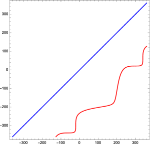
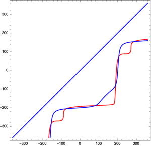
(a)	(b)
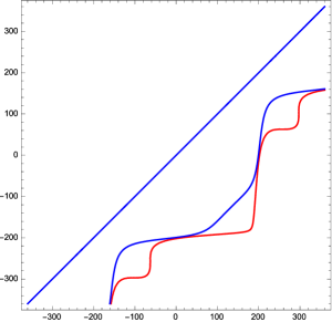
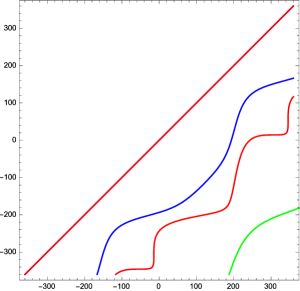
(c)	(d)
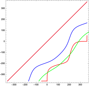
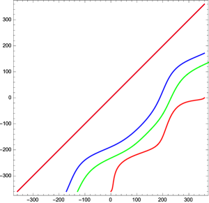
(e)	(f)

Figure 2: The boundaries ${\mathcal{C}}^{(n)}$ of the stability regions ${\sf C}_{n}$ for fixed CL for $n=0$ (red), $n=1$ (blue), $n=2$ (green), and a) $B=0.5$, b) $B=1.4$, c) $B=\pi/2$, d) $B=2.1$, e) $B=2.4$, f) $B=2.8$.

For $B>2$ we checked the influence of ${\mathcal{C}}^{(2)}$ on the shape of the stability region, and find out that it always lies outside of ${\sf C}_{1}$. The relative position of between ${\mathcal{C}}^{(0)}$ and ${\mathcal{C}}^{(2)}$ changes with $B$, namely, for $B$ values close to $2$ we observe ${\mathcal{C}}^{(2)}$ outside of ${\sf C}_{0}$, but with growth of $B$ is approaches ${\mathcal{C}}^{(0)}$, then intersects it and then ${\mathcal{C}}^{(2)}$ is completely between ${\mathcal{C}}^{(0)}$ and ${\mathcal{C}}^{(1)}$.

Thus, the numerical analysis implies that the stability region ${\sf C}$ for nodoids with fixed CL for $1<B<\pi/2$ is determined by interplay of the boundaries ${\mathcal{C}}^{(0)}$ and ${\mathcal{C}}^{(1)}$, while for larger values of $B$ it is completely defined by ${\mathcal{C}}^{(1)}$ only.

5.2 Stability region boundary for menisci with free CL

Turning to computation of the stability region for the menisci with free CL between two axisymmetric solid bodies one has first to establish the region of existence for the given meniscus (i.e., given values of $B$ and $S_{H}$) and the given SB (i.e., given ${\bf R}_{j}$). This region ${\sf Exist}(B,S_{H},{\bf R}_{1},{\bf R}_{2})$ is determined by a set of conditions (some of them are discussed in details in [15]). Then the construction of the boundaries ${\mathcal{B}}^{(n)}$ should be done only inside the existence region.

The method developed in [11] states that in order to establish the meniscus stability w.r.t. asymmetric perturbations it is sufficient to determine the boundary ${\mathcal{B}}^{(1)}$ of the first mode ($n=1$) only, except the case of the meniscus between two parallel plates when the boundary ${\mathcal{B}}^{(2)}$ for $n=2$ also should be taken into account. We start with this particular case.

5.2.1 Two parallel plates

It is easy to check that in this case $Z^{\prime}=Z^{\prime\prime}=R^{\prime\prime}=0,$ and $R^{\prime}=1,$ so that we find $\eta_{j}=z^{\prime}_{j},$ and $V_{j}=\eta^{\prime}_{j}$. The condition (4.15) reduces to

$$\eta_{j}w^{\prime(n)}(t_{j})=\eta^{\prime}_{j}w^{(n)}(t_{j}),\quad w^{(n)}(t_{j})=\eta_{j}=z^{\prime}_{j}.$$

Substitute it into (4.5) we obtain

$$(r\eta^{\prime})^{\prime}-\frac{n^{2}}{r}\eta-\frac{(rr^{\prime\prime})^{\prime}}{r^{\prime}}\eta=0.$$

Note that $\eta=z^{\prime}$ identically satisfies equation (4.5) with $n=1$. This means that the first mode boundary ${\mathcal{B}}^{(1)}$ does not exist, while ${\mathcal{B}}^{(n)}$ for $n>1$ should satisfy an meniscus existence condition $\eta_{j}=z^{\prime}(t_{j})=0,$ mentioned above. Using the explicit expression for $z^{\prime}(t)=(1+B\cos t)/r,$ we find the boundaries $t_{j}=t^{*},$ where $\cos t^{*}=-1/B$.

This result shows that the stability regions ${\sf Stab}_{0}$ found in [6] for unduloids between two parallel plates coincide with the stability regions ${\sf Stab}$ valid for arbitrary asymmetric perturbations. It also indicates that the boundary ${\mathcal{B}}^{(n)}$ of the stability region for the asymmetric perturbations exist only for nodoids ($B>1$), and this boundary coincides with the existence boundary of nodoids between two parallel plates. Thus, in this case the stability region ${\sf Stab}$ is determined by intersection of the stability region of the axisymmetric perturbation and the stability regions for asymmetric perturbation modes with fixed CL: ${\sf Stab}={\sf Stab}_{0}\cap{\sf C}$.

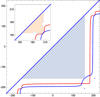
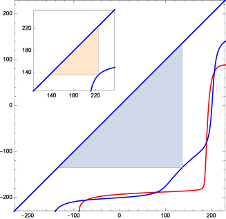
(a)	(b)

Figure 3: The stability region for nodoids with a) $B=1.1$ and b) $B=1.4$ between parallel plates. The shaded areas determine the stability region w.r.t. axisymmetric perturbations for the convex ($S_{H}=1$, blue) and concave ($S_{H}=-1$, orange) nodoids. Solid curves represent fixed CL stability boundary ${\mathcal{C}}^{(n)}$ for $n=0$ (red) and $n=1$ (blue).

The computations nevertheless show that ${\sf Stab}={\sf Stab}_{0}$ (see Figure 3); the boundary ${\mathcal{C}}^{(1)}$ only touches the region ${\sf Stab}_{0}$, but never intersects it. The contact point of ${\mathcal{C}}^{(1)}$ and ${\sf Stab}_{0}$ for the convex [concave] nodoid shown in Figure 3 is given by $t_{2}=t^{*},\;t_{1}=t^{*}[2\pi-t^{*}],$ when the matrix $D^{(1)}(t_{2},t_{1})$ is degenerate.

5.3 Influence of asymmetric perturbations on stability region

In [15] the stability regions for the axisymmetric menisci under axisymmetric perturbations were established for various geometrical settings. It is instructive to figure out how asymmetric perturbations affect these stability regions.

The condition (4.15) leads to the explicit expression for the stability boundary ${\mathcal{B}}^{(1)}$ of the first asymmetric perturbation mode

$$C_{11}C_{22}-C_{12}C_{21}=0,\quad C_{ij}=\eta_{j}w^{\prime(1)}_{i}(t_{j})-V_{j}w^{(1)}_{i}(t_{j}),$$ (5.2)

where $w^{(1)}_{i}$ are given by (4.6). In Appendix C we discuss a computational procedure determining the boundary ${\mathcal{B}}^{(n)}$ for asymmetric modes with $n>1$. The approach used in [11] implies that in order to find the stability region ${\sf Stab}_{1}$ for asymmetric perturbations it is enough to consider only a part of the boundary ${\mathcal{B}}^{(1)}$ that lies inside ${\sf C}_{1}$. Numerical simulations show that the boundary ${\mathcal{B}}^{(1)}$ in some cases might exist for arbitrary positive $B$. This means that both unduloid and nodoid stability regions might be reduced by asymmetric perturbations. Nevertheless, we did not find any combinations of the parameters for which the boundary ${\mathcal{B}}^{(1)}$ crosses the stability region for axisymmetric perturbations. The same time the boundary ${\mathcal{C}}^{(1)}$ does reduce the stability region of nodoid menisci with $B>1$. As an example we discuss below the stability of the nodoid menisci between two solid spheres.

5.3.1 Two equal spheres

For two spheres of the same radius $a$ we have $R_{j}=a\sin\tau_{j},\;Z_{j}=(-1)^{j}a\cos\tau_{j},$ where the angles $\tau_{j}$ parameterize the spherical surfaces and are found from the condition $R_{j}=r_{j},$ i.e., $a\sin\tau_{j}=\sqrt{1+B^{2}+2B\cos S_{H}t_{j}}$. It is easy to obtain the following relations:

$$\eta_{j}=\frac{aS_{H}}{r_{j}}\left[\cos\tau_{j}+B\cos(S_{H}t_{j}+(-1)^{j+1}\tau_{j})\right],\quad\tilde{V}_{j}=(-1)^{j+1}.$$

Substitution of these expressions and the solutions (4.6) into (5.2) produces an explicit condition for the boundary ${\mathcal{B}}^{(1)}$. We found that in some cases ${\mathcal{B}}^{(1)}$ can intersect ${\mathcal{C}}^{(1)}$, but it happens outside of the existence region. On the contrary, the curve ${\mathcal{B}}^{(1)}$ never crossed ${\sf Stab}_{0}$.

Figure 4 shows the stability regions for convex nodoid ($S_{H}=1$) between two equal solid spheres which demonstrates that only ${\mathcal{C}}^{(1)}$ but not ${\mathcal{B}}^{(1)}$ crosses the axisymmetric stability region ${\sf Stab}_{0}$.

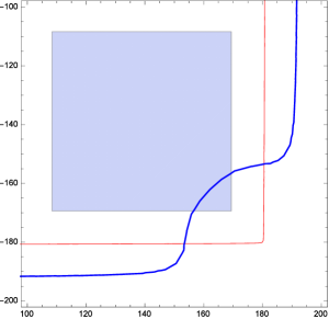
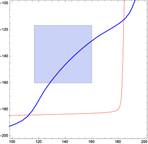
(a)	(b)

Figure 4: The stability region for nodoids with a) $B=1.05$ and b) $B=1.25$ between equal spheres with $a=1.2$. Blue shaded area determines the stability region w.r.t. axisymmetric perturbations. Solid curves represent fixed CL stability boundary ${\mathcal{C}}^{(n)}$ for $n=0$ (red) and $n=1$ (blue). The boundary ${\mathcal{B}}^{(1)}$ lies outside of the shown regions.

It is important to underline that asymmetric perturbations just reduce the stability region for the nodoids but not completely forbid their stability contrary to the statement in [20] that ”…a convex unduloidal bridge between two balls is a constrained local energy minimum for the capillary problem, and a convex nodoidal bridge between two balls is unstable”.

6 Discussion

In this manuscript we consider an extension of the analysis of axisymmetric menisci stability presented in [6] to the case of asymmetric perturbations. The method itself is a development of the Weierstrass’ general method valid in case of fixed CLs [21, 2]. The asymmetric perturbations in our approach presented as an expansion into the Fourier angular modes, the same way it was suggested in [11]. The stability analysis of the first perturbation mode is made analytically for all possible setups of the solid bodies. The case of arbitrary meniscus between two parallel plates is considered in Section 5.2.1, we found that its stability coincides with ${\sf Stab}_{0}$. Another significant conclusion of our computations is that there exist stable convex nodoids between two solid spheres.

Several important facts were established using numerical solutions of equation (4.5) with zero BC $w(t_{j})=0$ for menisci with fixed CL, and with mixed BC $(V_{j}/\eta_{j})w(t_{j})-w^{\prime}(t_{j})=0$ for menisci with free CL. These are:

1. The solution of Jacobi equation for $n$-th perturbation mode with fixed CL exists only for $B>n$.

2. For $n>0$ the boundary ${\mathcal{C}}^{(n+1)}$ lies outside the stability region ${\sf C}_{n}$, i.e., ${\sf C}={\sf C}_{0}\cap{\sf C}_{1}$.

3. For $n>0$ the boundary ${\mathcal{B}}^{(n+1)}$ lies outside the stability region ${\sf Stab}_{n}$, i.e., ${\sf Stab}={\sf Stab}_{0}\cap{\sf Stab}_{1}$.

Qualitatively similar result was obtained in [11] using the analysis of the eigenvalues spectrum of the SLE for an arbitrary perturbation mode. It would be very useful to have a proof of the abovementioned observations.

Appendix A Computation of $\chi_{j}$

Consider a derivation of an explicit expression for the parameter $\chi_{j}$ introduced in [11] for the computation of stability region. This quantity appears in the BC $\chi_{j}w^{(n)}(t_{j})+(-1)^{j}w^{\prime(n)}(t_{j})=0$. The definition of $\chi_{j}$ in [11] reads

$$\chi_{j}\sin\theta_{j}=\kappa_{j}\cos\theta_{j}-\bar{\kappa}_{j},$$ (A1)

where $\kappa_{j}$ and $\bar{\kappa}_{j}$ denote the planar curvature of the meridional cross sections of the meniscus and solid body, respectively, computed at the $j$-th contact point $t=t_{j}$, where $r(t_{j})=R_{j}(\tau_{j})$. The contact angle $\theta_{j}$ is determined as $\cos\theta_{j}=\langle{\bf t}_{j},{\bf T}_{j}\rangle/(|{\bf t}_{j}||{\bf T}_{j}|)$. As for the meniscus it holds that $|{\bf t}_{j}|=1,$ we can write

$$\cos\theta_{j}=(-1)^{j+1}\frac{R_{j}^{\prime}r_{j}^{\prime}+Z_{j}^{\prime}z_{j}^{\prime}}{\sqrt{R_{j}^{\prime 2}+Z_{j}^{\prime 2}}},\quad\sin\theta_{j}=\frac{z_{j}^{\prime}R_{j}^{\prime}-r_{j}^{\prime}Z_{j}^{\prime}}{\sqrt{R_{j}^{\prime 2}+Z_{j}^{\prime 2}}}=\frac{\eta_{j}}{\sqrt{R_{j}^{\prime 2}+Z_{j}^{\prime 2}}},$$ (A2)

where the prime ^′ denotes differentiation w.r.t. $t$ when it acts on ${\bf r}$ and w.r.t. $\tau$ when it acts on ${\bf R}$. The curvature $\kappa$ of the planar curve defined parametrically $\{r(t),z(t)\}$ reads $\kappa=(r^{\prime}z^{\prime\prime}-z^{\prime}r^{\prime\prime})/(r^{\prime 2}+z^{\prime 2})^{3/2},$ so that we obtain

$$\kappa_{j}=r_{j}^{\prime}z_{j}^{\prime\prime}-z_{j}^{\prime}r_{j}^{\prime\prime}=-r_{j}^{\prime\prime}/z_{j}^{\prime},\quad\bar{\kappa}_{j}=(-1)^{j+1}\frac{R_{j}^{\prime}Z_{j}^{\prime\prime}-Z_{j}^{\prime}R_{j}^{\prime\prime}}{(R_{j}^{\prime 2}+Z_{j}^{\prime 2})^{3/2}},$$ (A3)

where we use the relation $r_{j}^{\prime}r_{j}^{\prime\prime}+z_{j}^{\prime}z_{j}^{\prime\prime}=0$. Substituting (A3) into (A1) we find

$$\chi_{j}\eta_{j}=(-1)^{j+1}\left[R_{j}^{\prime}z_{j}^{\prime\prime}-Z_{j}^{\prime}r_{j}^{\prime\prime}-\frac{R_{j}^{\prime}Z_{j}^{\prime\prime}-Z_{j}^{\prime}R_{j}^{\prime\prime}}{R_{j}^{\prime 2}+Z_{j}^{\prime 2}}\right]=(-1)^{j+1}V_{j},\quad\chi_{j}=(-1)^{j+1}V_{j}/\eta_{j}.$$ (A4)

Appendix B Stability region ${\sf C}$ for menisci with fixed CL

In the case of fixed CL the solution $\bar{w}^{(n)}(t)$ of the Jacobi equation (4.5) with zero BC $\bar{w}^{(n)}(t_{j})=0$ can be expressed as a superposition of two fundamental solutions. When one of these two solutions, say, $\bar{w}^{(n)}_{2}$ is known, the other one can be found as $\bar{w}^{(n)}_{1}=U^{(n)}\bar{w}^{(n)}_{2},$ where $U^{\prime(n)}=g/(r[\bar{w}^{(n)}_{2}]^{2}),$ and $g$ is a constant depending on the parameter $B$ (see [6]). For example, for $n=1$ we have

$$U^{(1)}(t)=\frac{\bar{w}^{(1)}_{1}(t)}{\bar{w}^{(1)}_{2}(t)}=z(t)+\frac{r(t)r^{\prime}(t)}{z^{\prime}(t)}.$$

Using this representation in (5.1) we write it as $U^{(n)}(t_{1})=U^{(n)}(t_{2}),$ where $t_{1}>t_{2}$. For given $t_{2}$ introduce a function $\Psi^{(n)}(t)=U^{(n)}(t)-U^{(n)}(t_{2}),$ and write the condition on the boundary ${\mathcal{C}}^{(n)}$ as $\Psi^{(n)}(t^{(n)}_{1})=0$. As we have $\Psi^{\prime(n)}=U^{\prime(n)},$ this derivative retains its sign but it can diverge (when $\bar{w}^{(n)}_{2}=0$ or $r=0$ for a spherical meniscus at $B=1$). The condition $\bar{w}^{(n)}_{2}=0$ indicates that the function $\Psi^{(n)}(t)$ might vanish, so that a root $t^{(n)}_{1}$ exists. It is easy to see that for $n=1$ the relation $\bar{w}^{(n)}_{2}=0$ can be valid only for $B>1$, so that for unduloids the boundary ${\mathcal{C}}^{(1)}$ does not exist. For $B=n>1$ there are no boundaries ${\mathcal{C}}^{(k)}$ with $1\leq k\leq n$; it follows from the fact that $\tilde{w}^{(n)}_{2}(t)$ never vanishes while $\tilde{w}^{(n)}_{1}(t)$ is always positive.

For $n>1$ the solution of (4.5) with zero BC can be found numerically by employing the shooting method when the above conditions are replaced by $w^{(n)}(t_{2})=0,\;w^{\prime(n)}(t_{2})=1,$ used as initial conditions (IC) for numerical integration of equation (4.5). The resulting solution is used to find a value $t=t^{(n)}_{1}$ at which $w(t)$ vanishes, and (in case such a value exists) it provides a point $(t^{(n)}_{1},t_{2})$ belonging to the stability region boundary for $n$-th perturbation mode. The set of such points completely defines the boundary ${\mathcal{C}}^{(n)}$.

The computational analysis of equation (4.5) shows that $t^{(n)}_{1}$ exists only for $B>n$ (see Appendix D). It is instructive for given value of $t_{2}$ compare the values $t^{(n)}_{1}$ and $t^{(n+1)}_{1}$. It appears that it holds always that $t^{(n+1)}_{1}>t^{(n)}_{1},$ which implies that the boundary ${\mathcal{C}}^{(n+1)}$ lies outside of the region ${\sf C}_{n}$ bounded by ${\mathcal{C}}^{(n)}$. This observation indicates that the stability region ${\sf C}$ for menisci with fixed CL is determined exclusively by intersection ${\sf C}={\sf C}_{0}\cap{\sf C}_{1}$ of the regions for axisymmetric and first asymmetric modes. This result confirms the statement made in [11] about the stability region for the case of fixed CL.

Appendix C Stability region ${\sf Stab}$ for menisci with free CL

The relation (4.20) which determines the stability boundaries ${\mathcal{B}}^{(n)}$ employs matrices $A_{k}^{(n)}$ that depend on the fundamental solutions $w^{(n)}_{i}(t)$ and their derivatives. Using the representation $w^{(n)}_{1}(t)=U^{(n)}(t)w^{(n)}_{2}(t),$ we rewrite (4.20) for $n>0$ as

$$(U_{1}-U_{2})[V_{1}V_{2}-\eta_{1}G_{1}V_{2}+\eta_{2}G_{2}V_{1}+\eta_{1}\eta_{2}G_{1}G_{2}]-\eta_{1}V_{2}U^{\prime}_{1}+\eta_{2}V_{1}U^{\prime}_{2}+\eta_{1}\eta_{2}[G_{2}U^{\prime}_{1}-G_{1}U^{\prime}_{2}]=0,$$

where

$$U_{j}=U^{(n)}(t_{j}),\quad U^{\prime}_{j}=U^{\prime(n)}(t_{j}),\quad G_{j}=w^{\prime(n)}_{2}(t_{j})/w^{(n)}_{2}(t_{j}).$$

The above relation can be rewritten as

$$(U_{1}-U_{2})(V_{1}-\eta_{1}G_{1})(V_{2}-\eta_{2}G_{2})-\eta_{1}U^{\prime}_{1}(V_{2}-\eta_{2}G_{2})-\eta_{2}U^{\prime}_{2}(V_{1}-\eta_{1}G_{1})=0,$$

leading to the condition

$$\Phi_{1}=\Phi_{2},\quad\Phi_{j}=U_{j}-\frac{\eta_{j}U^{\prime}_{j}}{V_{j}-\eta_{j}G_{j}}.$$ (C1)

Returning to the original notation for the fundamental solutions we find a compact expression for (4.20) in the form

$$\Phi^{(n)}(t_{1})=\Phi^{(n)}(t_{2}),\quad\Phi^{(n)}(t)=\frac{Vw^{(n)}_{1}-\eta w^{\prime(n)}_{1}}{Vw^{(n)}_{2}-\eta w^{\prime(n)}_{2}}.$$ (C2)

It is easy to see that the condition (C2) is equivalent to (4.16) as expected. From the computational perspective the problem of finding a point $(t_{1},t_{2})$ belonging to the boundary ${\mathcal{B}}^{(n)}$ is reduced to a problem of finding the first zero $t^{(n)}_{1}>t_{2}$ of the function $\Psi^{(n)}(t)=\Phi^{(n)}(t)-\Phi^{(n)}(t_{2})$. Setting in (C2) $\eta=0$ we obtain $\Phi^{(n)}(t)=U^{(n)}(t),$ and we recover the condition for the stability boundary ${\mathcal{C}}^{(n)}$ derived in Appendix B for the menisci with fixed CL.

The numerical computations show that the stability boundary ${\mathcal{B}}^{(1)}$ might exist for $B<1$ but it appears that it does not intersect ${\sf Stab}_{0}$. This observation implies that asymmetric perturbations with free CL do not affect unduloid stability region ${\sf Stab}_{0}$ constructed using the analysis of axisymmetric perturbations only. In other words, for all unduloids we have ${\sf Stab}={\sf Stab}_{0}$, because any asymmetric perturbation is less dangerous than axisymmetric one. In case of nodoids with $B>1$ we found that ${\mathcal{B}}^{(1)}$ also does not intersect ${\sf Stab}_{0}$, so that only ${\mathcal{C}}^{(1)}$ might lead to reduction of the stability region.

Appendix D Analysis of Jacobi equation

Consider homogeneous Jacobi equation (3.16) and use a replacement $w=y/r$ to produce

$$r^{2}y^{\prime\prime}-rr^{\prime}y^{\prime}+(B^{2}-n^{2}+rz^{\prime})y=0.$$ (D1)

Substituting an ansatz $y=a_{0}+a_{1}\cos t+a_{2}\sin t,$ into (D1) we arrive at

$$[a_{0}(1+B^{2}-n^{2})-a_{1}B]-(a_{0}B-a_{1}n^{2})\cos t-a_{2}n^{2}\sin t=0,$$

which leads to a system

$$a_{0}(1+B^{2}-n^{2})-a_{1}B=0,\quad a_{0}B-a_{1}n^{2}=0,\quad a_{2}n^{2}=0.$$ (D2)

Direct substitution shows that for $n=0$ we have $a_{0}=a_{1}=0,$ and we reproduce the solution (4.4). With $n=1$ we find $a_{0}=1,\;a_{1}=B\;a_{2}=0,$ and we arrive at (4.6). Finally, setting $B=n,$ we obtain $a_{0}=B,\;a_{1}=1\;a_{2}=0,$ and generate the solution (4.7).

The IC $w_{1}(0)=0,\;w^{\prime}_{1}(0)=const>0,$ for (3.16) convert into $y_{1}(0)=0,\;y^{\prime}_{1}(0)=const>0,$ while the IC $w^{\prime}_{2}(0)=0,\;w_{2}(0)=const>0,$ lead to $y^{\prime}_{2}(0)=0,\;y_{2}(0)=const>0$. We performed numerical integration and found that for given value of $n$ the solutions to (D1) have qualitatively different behavior in two regions – $B<n,$ and $B>n$. These solutions are separated by the solution (4.7).

First, we found that for $B<n,$ both $y_{1}(t)$ and $y_{2}(t)$ are positive functions and for $t\gg 1$ it holds asymptotically that $y_{1}(t)\sim c(B,n)y_{2}(t),$ where positive constant $c$ depends on both $B$ and $n$. This observation implies that the function $\Psi^{(n)}$ introduced in Appendix C tends to constant for large $t$, and, moreover, we observe $\Psi^{(n)}\approx U^{(n)}$. This leads to a conclusion that ${\mathcal{C}}^{(n)}$ does not exist for $B<n,$ so that the stability region with fixed CL is found as ${\sf C}=\cap_{k=0}^{n-1}{\sf C}_{k}$.

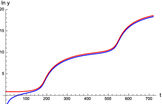
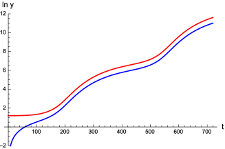
(a)	(b)

Figure 5: The logarithm of the fundamental solutions $\ln y_{1}(t)$ (blue) and $\ln y_{2}(t)$ (red) of the Jacobi homogeneous equation (3.16) for (a) $n=2,\;B=1.3,$ and (b) $n=3,\;B=2.3$.

In the other case $B>n,$ we observed that both $\bar{w}^{(n)}_{i}(t)$ change sign, so that the function $U^{(n)}$ changes sign too and thus the curve ${\mathcal{C}}^{(n)}$ exists. Similarly, the function $\Psi^{(n)}$ changes sign and its first zero determines the curve ${\mathcal{B}}^{(n)}$. The numerical simulations showed that the first root of the function $U^{(n)}$ can be approximated by $t^{(n)}_{1}\approx a(n)/\sqrt{\epsilon},$ where $0<\epsilon=B-n\leq 1,$ and $a(n+1)>a(n)$. A similar dependence of $t^{(n)}_{1}-t_{2}\approx a(n)/\sqrt{\epsilon}$ is valid for nonzero $t_{2}$. This implies that $t^{(n+1)}_{1}-t_{2}>t^{(n)}_{1}-t_{2}$ for all $n>0$, and the boundary ${\mathcal{C}}^{(n+1)}$ lies outside of the region ${\sf C}_{n}$ bounded by ${\mathcal{C}}^{(n)}$.

References

- [1] A. Beer, Tractatus de Theoria Mathematica Phenomenorum in Liquidis Actioni Gravitatis Detractis Observatorum, p. 17, George Carol, Bonn, 1857.
- [2] O. Bolza, Lectures on the Calculus of Variations, Univ. Chicago Press, 1904.
- [3] O. Bolza, Vorlesungen über Variationsrechnung, Leipzig und Berlin: B. G. Teubner Verlag, 1909.
- [4] C. E. Delaunay, Sur la surface de révolution dont la courbure moyenne est constante, J. Math Pure et App., 16 (1841), 309-315.
- [5] M.A. Erle, R.D. Gillette and D.C. Dyson, Stability of interfaces of revolution - the case of catenoid, Chem. Eng. J., 1 (1970), 97-109.
- [6] L.G. Fel, B.Y. Rubinstein, Stability of axisymmetric liquid bridges, Z. Angew. Math. Phys., s00033-015-0555-5 (2015).
- [7] A.R. Forsyth, Calculus of Variations, CUP, 1927.
- [8] R.D. Gillette and D.C. Dyson, Stability of fluid interfaces of revolution between equal solid plates, Chem. Eng. J., 2 (1971), 44-54.
- [9] A. Knesser, Lehrbuch der Variationsrechnung, Braunschweig, 1900 Archivum Mathematicum, 43 (2007), 417-429.
- [10] W. Howe, Rotations-Flächen welche bei vorgeschriebener Flächengrösse ein möglichst grosses oder kleines Volumen enthalten, Inaug.-Dissert., Friedrich-Wilhelms-Universität zu Berlin, 1887.
- [11] A.D. Myshkis, V.G. Babskii, N.D. Kopachevskii, L.A. Slobozhanin and A.D. Tyuptsov, Lowgravity Fluid Mechanics, Springer-Verlag, New York, 1987.
- [12] F. M. Orr, L. E. Scriven and A. P. Rivas, Pendular rings between solids: meniscus properties and capillary forces, J. Fluid Mech., 67 (1975), 723-744.
- [13] J. A. F. Plateau, Statique expérimentale et théoretique des liquides, Gauthier-Villars, Paris, 1873.
- [14] B.Y. Rubinstein and L.G. Fel, Theory of axisymmetric pendular rings, J. Colloid Interf. Sci., 417 (2014), 37-50.
- [15] B.Y. Rubinstein and L.G. Fel, Stability of unduloidal and nodoidal menisci between two solid spheres, Geometry and Symmetry in Physics, 39 (2015), 77-98.
- [16] L.A. Slobozhanin, Problems of stability of an equilibrium liquid encountered in space technology research, in Fluid mechanics and heat-and-mass transfer under zero gravity, Nauka, Moscow, 1982, 9-24 [in Russian].
- [17] M. Sturm, Note, Á l’occasion de l’article précédent, J. Math. Pure et App., 16 (1841), 315-321.
- [18] T. Vogel, Stability of a liquid drop trapped between two parallel planes, SIAM J. Appl. Math., 49 (1987), 516-525.
- [19] T. Vogel, Non-linear stability of a certain capillary problem, Dynamics of Continuous, Discrete and Impulsive Systems, 5 (1999), 1-16.
- [20] T. Vogel, Convex, rotationally symmetric liquid bridges between spheres, Pacific J. Math., 224 (2006), 367-377.
- [21] K. Weierstrass, Mathematische Werke von Karl Weierstrass. Vorlesungen über Variationsrechnung, Leipzig, Akademische Verlagsgesellschaft M.B.H., 1927.
- [22] L. Zhou, On stability of a catenoidal liquid bridge, Pacific J.Math., 178 (1997), 185-198.