Meta classification for variable stars

Abstract

The need for the development of automatic tools to explore astronomical databases has been recognized since the inception of CCDs and modern computers. Astronomers already have developed solutions to tackle several science problems, such as automatic classification of stellar objects, outlier detection, and globular clusters identification, among others. New science problems emerge and it is critical to be able to re-use the models learned before, without rebuilding everything from the beginning when the science problem changes. In this paper, we propose a new meta-model that automatically integrates existing classification models of variable stars. The proposed meta-model incorporates existing models that are trained in a different context, answering different questions and using different representations of data. Conventional mixture of experts algorithms in machine learning literature can not be used since each expert (model) uses different inputs. We also consider computational complexity of the model by using the most expensive models only when it is necessary. We test our model with EROS-2 and MACHO datasets, and we show that we solve most of the classification challenges only by training a meta-model to learn how to integrate the previous experts.

1. Introduction

The scientific community is dealing with massive amounts of digital information and astronomy is not an exception (see for example [Cook et al., 1995, Derue et al., 2002, Kaiser, 2004, Ivezic et al., 2008, Udalski et al., 2008]). It is practically impossible to analyze the vast amount of data, generated by modern telescopes and surveys, without the help of machines. This is done either with the use of simple algorithmic solutions or machine learning approaches. A particular example of such automatic methods is the automatic classification of variable objects [Richards et al., 2011, Bloom and Richards, 2011, Bloom et al., 2011, Kim et al., 2012, Pichara et al., 2012, Pichara and Protopapas, 2013], which is the focus of this paper. Automatic classification of variable stars makes it possible to speed scientific discoveries through an initial labelling, thus allowing astronomers to have a selection of lightcurves of interest for further study and analysis. Many solutions in automatic classification have been proposed [Richards et al., 2011, Long et al., 2012, Pichara et al., 2012, Butler and Bloom, 2011, Kim et al., 2014]. These models, called experts in this paper, classify to a subset of possible classes, using a set of specific variables (hereinafter called features) that represent the lightcurves. In this work, we aim that future models can take advantage of those models in solving new challenges. As an example, suppose that we have the following models:

• A model that classifies objects in quasars and no-quasars, trained with a specific set of features [Kelly et al., 2009, Kim et al., 2012, Pichara et al., 2012].

• A model that separates periodic from non-periodic objects [Huijse et al., 2012, Protopapas et al., 2015, Kim et al., 2014].

• A general purpose classifier that can classify (with a bit lower accuracy) many different variability classes [Richards et al., 2011, Long et al., 2012, Pichara and Protopapas, 2013].

• A model that classifies RR Lyrae [Gran et al., 2015] from the rest.

• A model that identifies microlensing and eclipsing binaries [Belokurov et al., 2003].

Assuming we need to create a model that classifies RR Lyrae, Eclipsing Binaries, Be stars, and quasars, it is apparent that there is a lot of intersection between the new desired model and the previous models we have. Therefore, we should be able to solve our new challenge without the need to build a totally new model.

The idea of mixing many different models is very old in machine learning literature [Jordan and Jacobs, 1993, Rasmussen and Ghahramani, 1991, Meir, 1996, Breiman, 2001, Kuncheva, 2007, Kuncheva and Whitaker, 2003, Bishop and Svensen, 2012, Chamroukhi, 2015]. These approaches are guided by the ‘divide and conquer’ principle, in which each expert focuses on a particular area of feature space. Most of the solutions proposed from machine learning literature assume the same context for each of the experts. In other words, they deal with data represented in the same feature space (same variables describing the data), and in most of the cases with the same set of predicted classes. To the best of our knowledge, there is not a mixture of experts solution that combines all the context variants we mention before, together with the efficient management of the computational complexity of the experts.

Our approach is based on a very simple idea of empirically estimate how fit a model is in a given scenario. In other words, the best we can do in learning how to combine different experts is to try them in different cases and evaluate their results. This idea allows us to avoid the need for the understanding of the internal structure of the experts, which can be very costly. Our approach first creates a meta-dataset containing all the experts’ outputs obtained from the initial training dataset. We search for patterns in the classification results and we model these patterns to predict the lightcurve classes. This is the meta-classifier, which integrates the outputs from the experts to make a final prediction.

The idea of studying models outputs was used before, but in different contexts, such as anomaly detection [Nun et al., 2014] and measurements of diversity [Kuncheva and Whitaker, 2003].

Furthermore, the integration model has to be easily understood and interpretable. It is not desirable to have a ‘black box’ that integrates the decision in an unknown and confusing way because we can not gain intuition on how the model is deciding, and how each expert is contributing to the final decision. Decision trees are very suitable for simple decision patterns; each node represents a question, and each directed edge pointing out from a node represents an answer from the node. There are many algorithms proposed to train a decision tree [Quinlan, 1986, 1993], but those algorithms just focus on optimising the classification accuracy rather than consider the cost of each question done on each of the nodes.

There are many known techniques that aim to describe lightcurves as vectors of real numbers (features) by trying to extract the maximum information from lightcurves while maximizing the classification performance. In a recent work, Nun et al. [2015] presented an automatic tool that calculates more than 60 such features. Depending on the classification task, some features are more useful than others, and some features are more computationally costly than others. One example of computationally costly features are the coefficients for a continuous autoregressive model [Kelly et al., 2009, Pichara et al., 2012]. However, these features have been shown to be helpful in differentiating quasars from other stars. Another example is the correntropy kernelized periodogram [Huijse et al., 2012], which has been used to classify periodicity classes. Both kinds of features are more expensive than others, but both present significant improvements in the classification tasks.

In our mixture of experts set up, each of the models solves different problems using different features with different estimation cost. The cost of classification from the mixture of experts can be calculated. Every time we ask a model to classify a given lightcurve, we know the features used by that model, and we either empirically measure or estimate the cost of each feature evaluation. Our meta-model deals with the experts’ cost by minimizing the overall cost. The algorithm considers besides the classification accuracy of each expert, their cost.

This work is organized as follows: In section 2 we present a brief description of the current research in mixtures of experts and related topics. In section 3 we give all the details of the proposed methodology. In section 4 we describe the experimental results obtained in different tests with real datasets. Finally in section 5 we discuss the main results of our work.

2. Related work

There are dozens of different methodologies to improve classification rates by combining the “expertise” of different classifiers. This whole topic is known in the machine learning community as ensemble learning or mixture of experts [Bishop, 2006, Jordan and Jacobs, 1993]. One of the earliest discussions of ensemble learning appears in the work of Bazell and Aha [2001], in which they combine different instances of the same model via bootstrapping, train each classifier in a randomly chosen sub-sample of the training set, and finally predict through majority voting.

The work from Freund et al. [1999] introduce the Adaboost algorithm, which combines classifiers in a cascade scheme. In the cascade of classifiers, each model trains only with the instances that the previous model predicted wrongly. This is achieved by tuning hyperparameters that control the false positive rate and the minimum acceptable detection rate. Unfortunately, this method works only for the two class problem though there are works that discuss extensions to multi-classes [Lin and Liu, 2005, Zehnder et al., 2008].

Although this ensemble method achieves good classification rates, it cannot be applied to our problem. This is because the combination and the classifiers are trained together; classifiers are not already trained. In our case, experts are already trained, and we do not need to train them again. On the contrary, we desire to re-use previously acquired knowledge. Moreover, most of boosting methods assume that instances of each model are represented through the same feature space (they use the same features on every model), and the predicted classes for every model are also the same. In our case, we use different features for each model and different output classes.

In Faraway et al. [2014] they have some similarity to our work in the sense that one of the classifiers they consider is hierarchical. They first evaluate if the object is a transient or not, and depending on the answer they attempt to classify among the other classes. What makes a big difference is that we propose a model that automatically learns that hierarchy and able to create different hierarchical classifiers depending on the case. On the other hand, Faraway et al. [2014] define a hierarchical classifier where the structure is set by hand and there is no any learning process about that hierarchy.

A seminal work in the mixture of experts was proposed in [Jordan and Jacobs, 1994]. They create a hierarchy of base level models that specialize in separate areas of the input space. On each level of the hierarchy, each expert is combined by a gate function that learns a model-combination function that varies depending on the instance to be classified. The combination function assigns a weight to each model in the final prediction. In the original paper, this function is a multinomial distribution, but there exist extensions using probability models from the exponential family [Xu et al., 1995]. Unfortunately, like most of the current machine learning approaches in mixtures of experts, this method is not helpful for our proposes, because the gate functions and the base models are all trained together to create the effect of specialization/cooperation and therefore all the models must belong to the same problem context (features and classes).

Another perspective of ensemble modelling, in the context of meta-models, is the use of a technique called Stacked Generalization [Wolpert, 1992]. In this framework, each base model (or level-0 model, in the nomenclature of the cited work) is “fed” with the data and the output of these models is considered as an input for a meta-model (level-1 model). This essentially creates an Intermediate Feature Space [Kuncheva, 2004] where the second stage learning can be performed. In the work of Wolpert [1992] this is referred as level-1 dataset, and the level-0 dataset is where the level-0 models are trained. This process can be repeated an indefinite number of times. Intuitively, the meta-model objective is to correct the bias of the base models [LeBlanc and Tibshirani, 1996].

Most of the methods mentioned above, rather than focus on work reutilization they concentrate on the “divide and conquer” principle and they do not consider cost, making them hard to use in the framework we are addressing in this work. Furthermore, to the best of our knowledge, there are no work in the field of astronomy addressing the problem of automatically learn how to combine previously learned models. We believe that in the area of lightcurve classification, automatic integration can make important contributions, especially with the continuous growth of data and models.

3. Proposed Method

We start by assuming that we have $m$ already trained models $\{M_{1},M_{2},\ldots,M_{m}\}$, where each model $M_{i}$ correspond to a lightcurve classifier. Each classifier $M_{i}$ uses a specific set of features $F_{M_{i}}$ to represent the lightcurves and classifies each lightcurve into a set $C_{M_{i}}$ of possible classes. For example, $M_{0}$ can be a model that uses the features $F_{M_{0}}=\{Amplitude,Autocor-length,CAR-tau,FluxPercentileRatio\}$, and is able to classify them into $C_{M_{i}}=\{QSO,RRL,Be,Other\}$. Besides having the already trained models $\{M_{1},M_{2},\ldots,M_{m}\}$, we have a training set ($D_{N}$), corresponding to the data associated with the new classification problem, the one we need to solve with the trained models.

3.1. Creation of the Predictions Dataset

The first step of the process is to create a (meta) dataset containing the predictions of each model ($D_{P}$) associated to each of the lightcurves in $D_{N}$. The main purpose of $D_{P}$ is to have training data for the meta model. To create $D_{P}$, we just run each of the trained models getting their predictions on the training set $D_{N}$. Then, we save those predictions as rows in $D_{P}$ together with the real class label of the lightcurve. Figure 1 shows an example of this process for three given models.

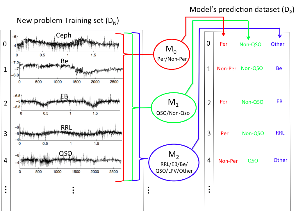
Figure 1.— Graphical description of the creation of models predictions data ($D_{P}$). We can see that starting from a set of labeled lightcurves ($D_{N}$) we ask to each model to predict the class to each of those lightcurves, then we record their predictions as new rows in $D_{P}$, generating a second dataset later used to train the mixture of models.

3.2. Meta model representation

After obtaining $D_{P}$, we can build a meta-model that efficiently mixes the decision of each of the previously trained models. The meta-model has to act as a “director”. Every time the meta-model receives a new query lightcurve, it has to choose who is the first model to be used, then depending on the prediction of that model, select the next model, and so forth. A natural representation of the meta-model is a decision tree structured schema, where each node represents one of the previously trained models $M_{i}$. Each of the edges pointing out from each node represents one of the possible predictions made from the model represented by the node, and leaves represent a final prediction done by the meta-model. Figure 2 shows an example with four models $\{M_{0},M_{1},M_{2},M_{3}\}$. The tree structure meta model first asks model $M_{2}$ to do the prediction. In the case that $M_{2}$ predicts a microlensing ($ML$), the meta-model immediately predicts $ML$ (reaches a leaf). In the case that model $M_{2}$ says $Non-ML$ the meta model asks model $M_{3}$ for a prediction. If $M_{3}$ predicts Cepheid ($CEPH$), RR Lyrae ($RRL$) or Eclipsing Binary ($EB$) the meta-model predicts according to $M_{3}$, but in the case that $M_{3}$ predicts $OTHERS$, the meta-model now asks $M_{1}$ for a prediction and so on. This kind of structure is very suitable for what we need. It is very easy to understand, uses a very well-known data structure from computer science (very mature searching and traversal algorithms), and the most important benefit is that it can be interpretable.

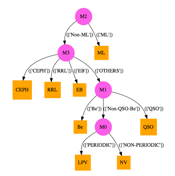
Figure 2.— Example of a meta model. Round nodes represent the previously trained models, edges show which path to follow depending on the model´s prediction, square nodes represent the leaves that correspond to a final prediction done by the meta-model.

3.3. Automatically building the meta model

After understanding the structure of the meta-model and how it works, the central question is how we build it? We propose an algorithm that is mainly driven by the probability that a given model correctly predicts the class of a lightcurve and the cost of running that model. The likelihood that a model correctly predicts the class of a given lightcurve can be estimated from the training data ($D_{P}$), and the cost of running that model can be easily calculated from the cost of all the features the model uses to represent the lightcurve.

The meta-model learning algorithm is inspired by the classical decision tree learning algorithm [Quinlan, 1986, 1993]. Given a score that measures the quality of any node, the best node is selected to be the root of the tree. Then the algorithm traverse down from each of the possible edges pointing out from the root (possible predictions of the model associated to the root) and recursively searches for the next best model. We select the best model ($M_{*}$) for a given node of the tree as follows:

$$M_{*}=\underset{M_{i}}{\arg\max}\;\frac{{\rm Info\_Gain}(M_{i})}{E\big{[}{\rm Cost}(M_{i})\big{]}},\;i\in[1,\ldots,m]$$ (1)

where ${\rm Info\_Gain}(M_{i})$ is the information gain [Quinlan, 1986] of model $M_{i}$, which measures the expected reduction in entropy in $D_{P}$ when model $M_{i}$ makes a prediction. It is defined as:

$${\rm Info\_Gain}(M_{i}) = H({\rm class})-\displaystyle\sum_{\begin{subarray}{c}v\in\\ C_{M_{i}}\end{subarray}}\frac{|v|}{|C_{M_{i}}|}H({\rm class}|v)$$

$$H({\rm class}) = -\sum_{k\in C^{M}}\frac{|k|}{|C^{M}|}\log\frac{|k|}{|C^{M}|}$$

$$H({\rm class}|v) = -\sum_{k\in C^{M}_{v}}\frac{|k|}{|C^{M}_{v}|}\log\frac{|k|}{|C^{M}_{v}|}$$ (2)

where $C^{M}$ is the union of all possible classes predicted among all models. Similarly, $C^{M}_{v}$ is the union of all classes predicted across the models $\{M_{1},M_{2},\ldots,M_{i-1},M_{i+1},\ldots,M_{m}\}$ when the model $M_{i}$ predicts $v$. In simpler words $H({\rm class}|v)$ is the entropy of the class column of $D_{P}$ selecting only the rows of $D_{P}$ that match $M_{i}=v$. Intuitively the information gain tell us if model’s $M_{i}$ predictions are good to separate among possible classes, in the sense that if every time we instantiate the model $M_{i}$ to it´s possible predictions, we see that the uncertainty in the class column is reduced or not (entropy). This concept is directly related to the probability of getting a successful classification if the meta-model uses $M_{i}$ to do the final prediction.

The term $E\big{[}{\rm Cost}(M_{i})\big{]}$ is the expected cost of a model, estimated as follows:

$$E\big{[}{\rm Cost}(M_{i})\big{]} = P_{L}(M_{i}){\rm Cost}(M_{i})+(1-P_{L}(M_{i}))\big{[}$$ (3)

$$\displaystyle\sum_{\begin{subarray}{c}v\in\\ C_{M_{i}}\end{subarray}}\sum_{j=i+1}^{m}P_{L}(M_{j}|M_{i}=v)\times$$

$$\times{\rm Cost}(M_{j}|M_{i}=v)\big{]}$$

The term $P_{L}(M_{i})$ indicates the probability that model $M_{i}$ reaches a leaf in the tree in the next step. In other words, how likely is that model $M_{i}$ will be making a final decision (reaching a leaf). Given that the decision tree algorithm creates a leaf every time most of the remaining instances belong to the same class, to estimate the probability of reaching a leaf we need an indicator of how good was the model after predicting a given class. This is also related to the information gain of the model at that level of the tree. To have valid probability values, we normalize the information gain from $[0,1]$ as:

$$P_{L}(M_{i}) \approx 1-\frac{\displaystyle\sum_{v\in C_{M_{i}}}\frac{|v|}{|C_{M_{i}}|}H({\rm class}|v)}{H({\rm class})}$$ (4)

The cost of model $M_{i}$ (${\rm Cost}(M_{i})$) is calculated as the sum of the features that model $M_{i}$ uses to represent each lightcurve. The second part of equation 3 is basically the weighted sum of every model but model $M_{i}$ cost, where each weight corresponds to the probability that the given model reaches a correct leaf in the tree in the next step. Intuitively, equation 1 is finding the model whose cost is minimum and at the same time take the meta-model models to the right prediction.

We summarize the training and predicting steps of the Meta-Classification process below :

Training:

• For each new model $M_{i}$ create a new data column $D_{P}[i]$ with the prediction of each model $M_{i}$ over the training data.

• Build $D_{P}$ as a union of all the predictions, $D_{P}=\bigcup_{i=1}^{m}D_{P}[i]$

• Create the meta-training set adding to $D_{P}$ a column with the known class of each object (this is just the same class column included in $D_{N}$).

• Build the meta-model according to section 3.3

Predicting:

• For any unclassified lightcurve $x$, start traversing the meta-model tree from the root

• On each node $M_{i}$, extract the features $F_{M_{i}}$, go down the tree according to the prediction of $M_{i}$ until a leaf is reached.

• Predict according to the reached leaf.

4. Experimental Results

We tested our model with two lightcurve datasets, MACHO [Cook et al., 1995] and EROS-2 [Tisserand et al., 2007]. On each dataset, we created different experts models trained to classify among different subsets variability classes. Each model in the setup uses a specific set of features to describe the lightcurves. These specific sets are determined using a feature importance algorithm called mean decrease impurity, described in Breiman et al. [1984]. After a particular model $M_{i}$ is trained, if the meta model requires a prediction from $M_{i}$, it only will extract the features included on $M_{i}$’s specific set. Note that if previously other model extracted some of the required features, they will not be extracted again.

For each of the experts we use a Random Forest classifier [Breiman, 2001]. We use FATS (Feature Analysis for Time Series; [Nun et al., 2015]) tool to extract the features of lightcurves. This tool is able to extract up to 64 different features per lightcurve. All details about the meaning of each of the features can be found in Nun et al. [2015]. As mentioned above, some of the features are more expensive than others. Since each expert uses a selection of the best features according to its own classification problem, models have different associated cost.

All the accuracy results are presented throughout recall, precision, F-score and confusion matrix. All these indicators were obtained using a 10-fold cross validation process on each of the training sets.

4.1. MACHO dataset

The MACHO Project (Massive Compact Halo Objects) [Cook et al., 1995] observed the Magellanic Clouds and Galactic bulge with the main purpose of detecting microlensing events. Observations were done using blue ($\sim$ 4500 to 6300Å) and red ($\sim$ 6300 to 7600 Å) passbands. The cadence is about 1 observation per 2-days for 7.4 years, which generates approximately 1000 observations per object. The lightcurves used in this work are from the Small and Large Magellanic Clouds. The fields cover almost the entire LMC bar (10 square degrees) to a limiting magnitude of V $\approx$ 22. The training set contains 6059 labeled lightcurves [Kim et al., 2011]. Table 1 shows the number of lightcurve per each of the available classes. We created seven models to work as experts, each one trained on a specific problem, with a specific set of features. Table 2 shows the features used on each model and the classes each model predicts.

class	# instances
Be stars	127
CEPH	101
EB	255
LPV	361
ML	580
NV	3963
QSO	59
RRL	613

Table 1Number of instances per each class of variability in MACHO training set

Name	Features used in the model	Possible classes	Avg. cost per lightcurve (secs)
$M_{0}$	Psi eta, StetsonL, Psi CS, PeriodLS, StetsonJ, Rcs, Period fit, StetsonK AC	PERIODIC, NON-PERIODIC	1.729
$M_{1}$	Rcs, Color, PeriodLS, Psi CS, Auto-cor-length, Mean, MedianAbsDev, StetsonJ, CAR tau, CAR mean, StetsonL, PercentDifferenceFluxPercentile, Q31, SlottedA length, Eta e, AndersonDarling, Con, FluxPercentileRatioMid65, Freq1 harmonics rel phase 1, Q31 color, Freq2 harmonics amplitude 2, Meanvariance, MedianBRP, Skew, MaxSlope	NON-QSO, QSO	2.554
$M_{2}$	Rcs, PeriodLS, Color, Autocor length, Psi CS, SlottedA length, StetsonL, Meanvariance, StetsonJ, PercentAmplitude, Amplitude, Std, Mean, Psi eta, CAR tau, FluxPercentileRatioMid65, Con, Freq3 harmonics amplitude 0	Non-QSO-Be, Be, QSO	2.551
$M_{3}$	Color, Con, SlottedA length, Mean, Rcs, StetsonK, Eta e, Skew	Non-ML, ML	0.823
$M_{4}$	Psi eta, PeriodLS, Rcs, Psi CS, CAR mean, StetsonL, CAR tau, Period fit, StetsonJ, FluxPercentileRatioMid35, Skew, Mean, Color	CEPH, RRL, EB, OTHERS	1.730
$M_{5}$	Psi eta, SlottedA length, Psi CS, StetsonJ, Color, StetsonL, Period fit, StetsonK AC, Con, Rcs, FluxPercentileRatioMid35, FluxPercentileRatioMid50, Eta e, Skew, Beyond1Std, FluxPercentileRatioMid80, FluxPercentileRatioMid65, FluxPercentileRatioMid20, PeriodLS, MedianBRP	CEPH, OTHERS, NV, EB	2.550
$M_{6}$	Color, Rcs, Skew, SlottedA length, Con, Psi CS, Psi eta, StetsonJ, PeriodLS, Eta e, StetsonK, FluxPercentileRatioMid35, Mean, Period fit, CAR mean, StetsonL, FluxPercentileRatioMid50, FluxPercentileRatioMid20, FluxPercentileRatioMid65, CAR tau, Autocor length, Q31 color, Beyond1Std	EB, OTHERS, Be, ML	2.552

Table 2Pre-trained models for MACHO dataset, features used on each model, classes that each model can predict and cost that each model takes to represent one lightcurve. The cost is directly related with the features models need to extract in order to classify a given lightcurve.

Table 3 presents the precision, recall and f-score of each of the classes per each of the models. Most of the models are getting high f-score for all their classes. We can see that quasars are the most complicated objects, mainly because they are confused with Be stars (model $M2$).

Model	Class	Precision	Recall	F-Score
M6	Be	0.733	0.780	0.756
	OTHERS	0.985	0.985	0.985
	ML	0.970	0.964	0.967
	EB	0.877	0.867	0.872
M0	PERIODIC	0.957	0.962	0.960
	NON-PERIODIC	0.989	0.988	0.989
M3	Non-ML	0.995	0.997	0.996
	ML	0.970	0.957	0.964
M2	Be	0.866	0.811	0.837
	QSO	0.738	0.525	0.614
	Non-QSO-Be	0.994	0.998	0.996
M4	CEPH	0.929	0.901	0.915
	RRL	0.967	0.949	0.958
	EB	0.900	0.878	0.889
	OTHERS	0.993	0.997	0.995
M1	NON-QSO	0.995	0.998	0.996
	QSO	0.675	0.458	0.545
M5	CEPH	0.936	0.871	0.903
	OTHERS	0.954	0.976	0.965
	EB	0.897	0.855	0.876
	NV	0.992	0.987	0.990

Table 3Accuracy indicators per each class on each of the models problem, in MACHO dataset.

After learning the meta model from the MACHO data using the proposed algorithm, we obtained the structure that is shown in Figure 3. We can see how the meta-model performs the classification. The meta-model starts by asking $M5$ and if $M5$ predicts “EB”, “CEPH” or “NV”, the meta-model predicts as $M5$ without asking any other model, but if $M5$ predicts “Others”, then the meta-model asks for the prediction from $M6$, and so on. From the tree, we can also see in most cases that the meta-model asks other models when the prediction is not so confident, like “Others” or when there is a hard class. For example, if $M6$ says that the object is a Be star, the meta-model does not predict immediately, but it continues and asks $M2$, which also knows about Be stars, and $M2$ predicts a Quasar (which usually is confused with Be stars); the meta-model also predicts a Quasar. If $M2$ predicts a Be star, the meta-model can also predict a Be star. A more interesting situation occurs when $M2$ predicts “Non-QSO-Be” (Non-Quasar and Non-Be star). In this case, the best decision the meta-model can do is to predict a Be star, which is more likely than any other class given that $M6$ predicted a Be star. It is also interesting to see that the meta-model can classify Long Period Variables (LPV) even if none of the previous models can classify them, mainly because from the training set the meta-model could infer prediction patterns from the models that occur together with the LPV class. From the tree, we can see that the meta-model is predicting LPV by discarding the other classes because most of the edges along the paths that end up in an LPV tree correspond to predictions for “Others” or “Non-$<$some classes$>$” from most of the models. Another very fascinating pattern happens with LPV; the meta-model realizes that LPV is a Periodic star, after the model $M0$ in the 4th level of the tree. Note also the meta-model does not use model $M1$. Model $M1$ classifies between Non-QSO and QSO, which are classes already covered by model $M2$.

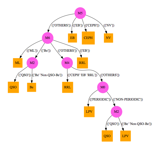
Figure 3.— Meta-model learned from the MACHO training set.

To show that the meta model does not sacrifice performance after the integration, Table 4 shows recall, precision and F-score of the final meta model. and in Figure 4 we can see the confusion matrix of the meta-classifier. Most of recall, precision and f-score values are maintained in the meta-classifier, even some indicators are improving, like in the case of Cepheids, as a result from the collaboration of two different models that are able to classify Cepheids.

Class	Precision	Recall	F-Score
Be	0.857	0.756	0.803
CEPH	0.936	0.871	0.903
EB	0.897	0.855	0.876
LPV	0.799	0.978	0.879
ML	0.977	0.960	0.969
NV	0.992	0.987	0.990
QSO	0.732	0.508	0.600
RRL	0.946	0.949	0.948

Table 4Accuracy indicators per each class for the meta-model, in MACHO training set.

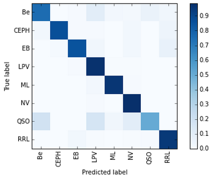
Figure 4.— Confusion matrix for the meta-model learned from the MACHO training set.

To show the contribution of the cost estimation of each model, we run the same experiment just considering the information gain in the score of each model, in other words, we assume that all models have the same cost. The resulting meta-model is shown in Figure 5. The meta-model, in this case, is less efficient, asking for a prediction more than once to most of the models, for example, independently of the prediction of model $M0$, the meta model asks twice for a prediction to $M1$. Also, note that this meta-model decides to use $M1$ instead of $M2$, which is a cheaper model but not necessarily worst than $M1$. As we can see from Table 5 and confusion matrix in Figure 6, there is no strong difference between the classification results; only in Cepheids we can see a 2% of improvement in the F-score when the meta-classifier does not penalize each model according to their cost, but there is a drop in F-score for the class Be stars. Calculating the total training cost for the meta-classifier in both cases (with and without considering the cost of the expert models), when the meta-model does not take into account the cost, the training process takes 167% longer than in the case when the meta-classifier takes into account the cost of the model experts.

Figure 5.— Meta-model learned from the MACHO training set without considering the of the models.

Class	Precision	Recall	F-Score
Be	0.832	0.740	0.783
CEPH	0.938	0.901	0.919
EB	0.884	0.863	0.873
LPV	0.779	0.978	0.867
ML	0.974	0.964	0.969
NV	0.993	0.985	0.989
QSO	0.667	0.441	0.531
RRL	0.954	0.938	0.946

Table 5Accuracy indicators per each class for the meta-model without considering the cost of models, in MACHO training set.

Figure 6.— Confusion matrix for the meta-model without considering the cost of the experts, learned from the MACHO training set.

4.2. EROS dataset

The EROS project (Expérience de Recherche d’Objets Sombres) [Derue et al., 1999] observed the Galactic Spiral Arms (GSA), LMC, SMC and Galactic bulge during 6.7 years, dedicated to detect microlensing events. Observations were done in two non standard passbands. One is the EROS-red passband $R_{\rm E}$, centred on $\bar{\lambda}=762\ {\rm nm}$ and EROS-visible passband $V_{\rm E}$, centred on $\bar{\lambda}=600\ {\rm nm}$. The lightcurves used in this work are from the LMC (60 fields) and SMC (10 fields). The limiting magnitud of the EROS $V_{\rm E}$ band is $\sim$ 20. The cadence varies among the fields, but in average about 500 observations were obtained for each lightcurve. The training set contains 68,718 labeled lightcurves, obtained from Kim et al. [2014]. Table 6 shows the number of lightcurves per each of the available classes. This training set is more complex than MACHO training set, in the sense that some subclasses of variability are added to the problem, making the separation more challenging due to the similarity among some classes. Our main goal is not to solve the classification problem for all the subclasses but to solve the integration problem using the provided expert models. Therefore, in cases where the respective experts do not well classify some subclasses, the meta-model will probably not be able to classify well those classes either. We used six model experts, each one trained on a specific problem, with a specific set of features. Table 7 shows the features used on each model, the available classes each model can predict and the average cost per lightcurve that the model takes to perform classification.

class	# instances
Ceph 1O	870
Ceph F	1272
Ceph 1O 2O	111
EB	13523
LPV OSARG RGB O	31487
LPV SRV AGB O	4337
LPV SRV AGB C	3748
LPV Mira AGB C	760
LPV Mira AGB O	320
RRL	12167
T2CEPH	123

Table 6Number of instances per each class of variability in EROS training set.

Name	Features used in the model	Possible classes	Avg. cost per lightcurve (secs)
$M_{0}$	Color, Mean, PeriodLS, CAR mean, Q31 color, Autocor length, CAR tau, FluxPercentileRatioMid50, FluxPercentileRatioMid35, SlottedA length, FluxPercentileRatioMid65, Rcs, Q31, MedianAbsDev, FluxPercentileRatioMid20, Beyond1Std, CAR sigma, Amplitude, Psi eta	OTHERS, CEPHEID, RRL, EB	16.326
$M_{1}$	Color, Mean, CAR mean, Autocor length, Q31 color, CAR tau, SlottedA length, PeriodLS, Rcs, CAR sigma, Amplitude, PercentDifferenceFluxPercentile	LPV, Non-LPV	16.325
$M_{2}$	Color, Mean, PeriodLS, CAR mean, Q31 color, CAR tau, FluxPercentileRatioMid50, SlottedA length, FluxPercentileRatioMid35, Autocor length, FluxPercentileRatioMid65, FluxPercentileRatioMid20, CAR sigma, Rcs, Q31, MedianAbsDev, Beyond1Std, Amplitude, Freq1 harmonics amplitude 0, Psi eta	OTHERS, RRL, CEPH T2CEPH, EB	21.644
$M_{3}$	PeriodLS, Mean, Color, FluxPercentileRatioMid50, Q31, FluxPercentileRatioMid35, Q31 color, MedianAbsDev, CAR mean, FluxPercentileRatioMid65, CAR tau, Freq1 harmonics amplitude 0, FluxPercentileRatioMid20, Beyond1Std, Std, StetsonK, Rcs, SlottedA length, StetsonL, FluxPercentileRatioMid80, PercentDifferenceFluxPercentile, Amplitude	OTHERS, Ceph 1O 2O, RRL, Ceph 1O, T2CEPH, Ceph F	7.866
$M_{4}$	Color, Mean, Q31 color, SlottedA length, PercentDifferenceFluxPercentile, CAR mean, Amplitude, Autocor length, Q31, Std, CAR tau, MedianAbsDev, Meanvariance, StetsonJ, Freq1 harmonics amplitude 0, PeriodLS, Rcs	OTHERS, LPV OSARG RGB O, LPV Mira AGB C, LPV SRV AGB O, LPV SRV AGB C, LPV Mira AGB O	7.866
$M_{5}$	PeriodLS, Mean, Color, FluxPercentileRatioMid50, FluxPercentileRatioMid35, MedianAbsDev, Q31 color, Q31, CAR mean, Freq1 harmonics amplitude 0, FluxPercentileRatioMid20, FluxPercentileRatioMid65, CAR tau, Beyond1Std, Autocor length, FluxPercentileRatioMid80, SlottedA length, StetsonK, Std, Skew, StetsonL	OTHERS, CEPHEID, RRL	7.867

Table 7Pre-trained models for EROS dataset, features used on each model, classes that each model can predict and cost that each model takes to represent one lightcurve. The cost is directly related with the features models need to extract in order to classify a given lightcurve.

Table 8 shows the precision, recall and f-score of each of the classes per model. As we can see, in some cases the experts failed to classify some of the classes. For example, $M3$ it not able to successfully classify T2 Cepheids and also the f-score for Cepheids 1O 2O is lower than the average score of the other models and classes. This setup, in particular, is showing us that some of the variability classes can not be automatically classified by the expert, making the meta-model learning process harder than the setup with MACHO dataset.

Model	Class	Precision	Recall	F-Score
M5	RRL	0.960	0.938	0.949
	OTHERS	0.985	0.991	0.988
	CEPHEID	0.962	0.952	0.957
M1	LPV	0.992	0.996	0.994
	Non-LPV	0.994	0.988	0.991
M0	RRL	0.965	0.937	0.951
	CEPHEID	0.957	0.957	0.957
	OTHERS	0.992	0.995	0.993
	EB	0.939	0.954	0.946
M3	RRL	0.957	0.938	0.947
	T2CEPH	0.944	0.545	0.691
	Ceph 1O 2O	0.758	0.676	0.714
	Ceph 1O	0.926	0.860	0.892
	Ceph F	0.965	0.965	0.965
	OTHERS	0.984	0.991	0.988
M2	RRL	0.966	0.938	0.952
	CEPH T2CEPH	0.988	0.948	0.968
	OTHERS	0.992	0.997	0.994
	EB	0.940	0.956	0.948
M4	LPV Mira AGB C	0.872	0.867	0.869
	LPV SRV AGB C	0.947	0.921	0.934
	LPV OSARG RGB O	0.974	0.989	0.982
	LPV SRV AGB O	0.901	0.863	0.882
	OTHERS	0.994	0.989	0.992
	LPV Mira AGB O	0.904	0.794	0.845

Table 8Accuracy indicators per each class on each of the models problem, in EROS dataset.

Figure 7 shows the resulting meta-model for EROS training set. We can see that at the root level, the meta-model asks $M4$ for a classification, in cases where $M4$ predicts LPV-SRV-AGB-C, LPV-Mira-AGB-C, LPV-Mira-AGB-O and LPV-SRV-AGB-O, the meta-model believes $M4$, in other cases it asks for other predictions. That makes sense because $M4$ is the only model trained to separate the subclasses of LPVs. In some cases the meta-model wants to get more confident about the prediction of some of the LPV subclasses, asking other models and predicting again the LPV subclasses when most of the other models predict “Others”. When $M4$ predicts LPV-OSARG-RGB-O, the meta-model asks more before taking a final decision. For example asking to $M0$, and in cases where $M0$ is not so confident about one of its classes and predicts “Others”, the meta-model predicts according to $M4$. Other model that contributes with extra information about the LPV stars is $M1$, which can predict between “LPV” or “Not-LPV”. We can see from the tree that in some cases the meta-model ends up predicting a subclass of LPV´s after most of the models predict “Others” and $M1$ predicts a LPV. It is interesting to see how the meta-model takes advantage of having more experts trained to classify RR Lyrae stars. For example, after $M4$ predicts “Others”, the meta-models asks for $M3$, and when $M3$ predicts a RR Lyrae, instead of immediately believing to it, the meta-model asks to $M2$, and again if $M2$ predicts a RR Lyrae, the meta model also predicts RR Lyrae. More interesting is when $M4$ says “Others” and $M3$ also says “Others”, if $M2$ predicts a RR Lyrae, the meta-model instead of immediately believe to $M2$ asks for a prediction to $M5$, and if $M5$ confirms that it is a RR Lyrae, then the meta-model also predicts a RR Lyrae.

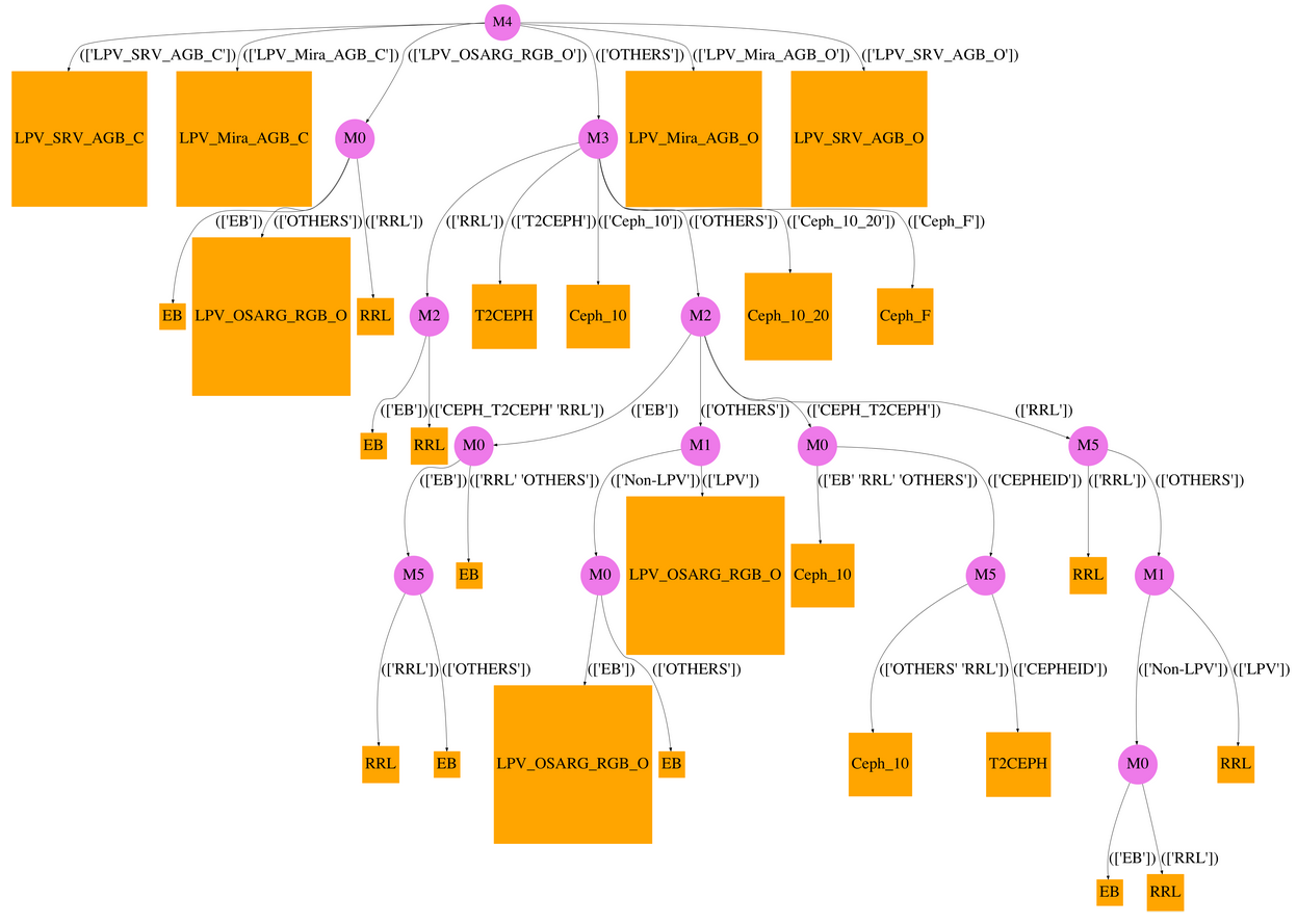
Figure 7.— Big picture of the Meta-model learned from the EROS training set.

To show that the meta model does not sacrifice performance after the integration, Table 9 shows recall, precision and F-score of the final meta model. In Figure 8 we can see the confusion matrix of the meta-classifier. Most of recall, precision and f-score values are maintained in the meta-classifier.

Class	Precision	Recall	F-Score
Ceph 1O	0.901	0.878	0.889
Ceph 1O 2O	0.758	0.676	0.714
Ceph F	0.965	0.965	0.965
EB	0.938	0.954	0.946
LPV Mira AGB C	0.872	0.867	0.869
LPV Mira AGB O	0.904	0.794	0.845
LPV OSARG RGB O	0.974	0.990	0.982
LPV SRV AGB C	0.947	0.921	0.934
LPV SRV AGB O	0.901	0.863	0.882
RRL	0.965	0.938	0.951
T2CEPH	0.893	0.545	0.677

Table 9Accuracy indicators per each class for the meta-model, in EROS training set.

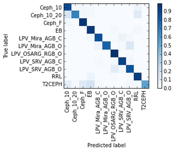
Figure 8.— Confusion matrix for the meta-model learned from the EROS training set.

As we did in the MACHO experiment, in EROS we also run the same experiment without considering the cost of each model. The resulting meta-model is shown in Figure 9. Similarly to that in the MACHO case, the meta-model asks many times for a prediction to most of the models, trying to maximize the confidence about the prediction instead of counting how expensive is the process. The meta-model basically asks all the models that can contribute with some information about certain classification, maximizing the confidence without restriction in the number of questions it does. We can see for example that models $M3$ and $M5$ are the most expensive models (Table 7), so the meta-model that takes into account the cost, does not call to $M3$ and $M5$ as much as the meta-model without cost does. From Table 10 and confusion matrix in Figure 10, we can see that there is no significative improvement in f-score in the meta-model that does not consider the cost. Calculating the total training cost for the meta-classifier in both cases (with and without considering the cost of the expert models), when the meta-model does not take into account the cost, the training process takes about 80% longer than in the case when the meta-classifier takes into account the cost of the model experts.

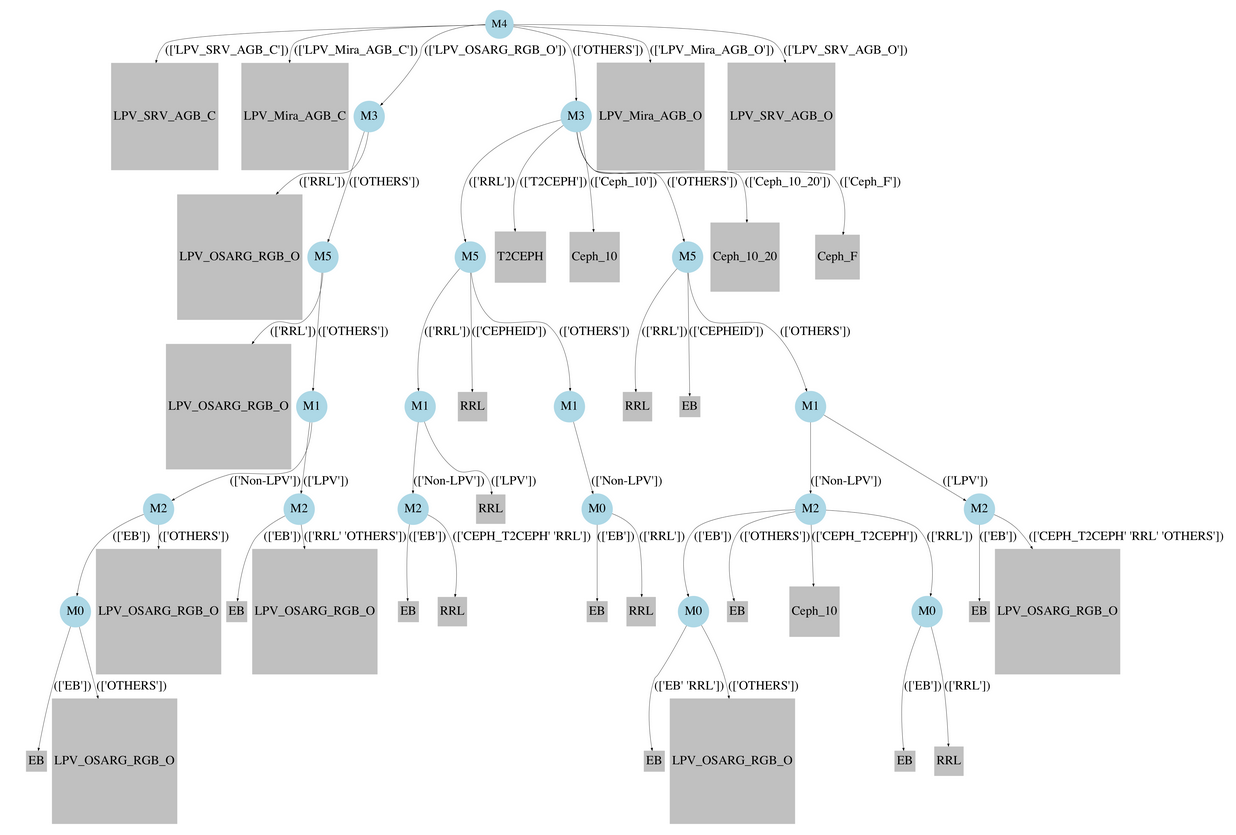
Figure 9.— Meta-model learned from the EROS training set without considering the of the models.

Class	Precision	Recall	F-Score
Ceph 1O	0.910	0.876	0.893
Ceph 1O 2O	0.758	0.676	0.714
Ceph F	0.962	0.965	0.963
EB	0.936	0.955	0.945
LPV Mira AGB C	0.872	0.866	0.869
LPV Mira AGB O	0.904	0.794	0.845
LPV OSARG RGB O	0.973	0.990	0.982
LPV SRV AGB C	0.947	0.921	0.934
LPV SRV AGB O	0.901	0.863	0.882
RRL	0.966	0.936	0.951
T2CEPH	0.931	0.545	0.687

Table 10Accuracy indicators per each class for the meta-model without considering the cost of models, in EROS training set.

Figure 10.— Confusion matrix for the meta-model without considering the cost of the experts, learned from the EROS training set.

5. Conclusions

We present a novel algorithm that allows astronomers to solve new classification problems by reusing previously trained classifiers. This kind of solutions facilitate a faster development of automated classification methodologies, avoiding to re-train new models from scratch. Upcoming surveys like LSST [Ivezic et al., 2008] will demand this kind of solutions, since the amount of data will not allow scientists to waste time re-calibrating models every time new science problems appear. Our intuition is that when a new variable star classification problem arises, if there are classes of stars and features already involved in previous problems, we should be able to use those models in the building process of the new solution. So far most of the research done in the automatic classification of variable stars field show strong relationships among the classes they study and the features they use, any of those classifiers could be plugged into our meta algorithm and be used to build a new solution. An important contribution of this work relies in the possibility to work with different contexts, something that is very natural when model integration occurs; every model has to deal with its own classes and its own data representation, which makes the integration more challenging. So far we have very promising results, the accuracy of the meta-model was as good as the accuracy of the model experts, that is the first goal that a integration model has to achieve.

Another important contribution is that the meta-model is human readable, we can easily observe the meta-model structure, directly inferring how the meta-model acts on every possible situations, making the meta-model more trustable for scientists. As future research we aim to work on the integration of data coming from different kind of telescopes, this creates new challenges to overcome, such as the identification of hidden patterns that come from instrumental differences, and the application of those patterns to the classification models to make them able to work on heterogeneous data. We strongly believe that making efforts in that direction will have a huge impact in the astronomical community. An issue that is not addressed in this work is the fact that the training sets are unbalanced and not properly evaluated. Analysing and generating better training sets is a future research direction. As a matter of fact, there are no good descriptions on how most of the training sets were generated in the first place. For this work, we assume the training sets are given. Fortunately, from the results we can see that Random Forest classifier can deal with unbalanced training sets. The k-fold cross validation process we use is stratified, ensuring that the testing and training sets are created with the same proportions of stars as the initial variability classes.

References

- Bazell and Aha [2001] D. Bazell and David W. Aha. Ensembles of Classifiers for Morphological Galaxy Classification, 2001. ISSN 0004-637X.
- Belokurov et al. [2003] V. Belokurov, N. W. Evans, and Y. L. Du. Light-curve classification in massive variability surveys – I. Microlensing. Monthly Notices of the Royal Astronomical Society, 341(4):1373–1384, jun 2003. ISSN 0035-8711. 10.1046/j.1365-8711.2003.06512.x. URL http://arxiv.org/abs/astro-ph/0211121.
- Bishop [2006] Christopher M Bishop. Pattern Recognition and Machine Learning, volume 4. 2006. ISBN 9780387310732. 10.1117/1.2819119. URL http://www.library.wisc.edu/selectedtocs/bg0137.pdf.
- Bishop and Svensen [2012] Christopher M. Bishop and Markus Svensen. Bayesian Hierarchical Mixtures of Experts. oct 2012. URL http://arxiv.org/abs/1212.2447.
- Bloom and Richards [2011] J.~S. Bloom and J.~W. Richards. Data Mining and Machine-Learning in Time-Domain Discovery {amp} Classification. ArXiv e-prints, 2011.
- Bloom et al. [2011] J.~S. Bloom, J.~W. Richards, P.~E. Nugent, R.~M. Quimby, M.~M. Kasliwal, D.~L. Starr, D Poznanski, E.~O. Ofek, S.~B. Cenko, N.~R. Butler, S.~R. Kulkarni, A Gal-Yam, and N Law. Automating Discovery and Classification of Transients and Variable Stars in the Synoptic Survey Era. ArXiv e-prints, 2011.
- Breiman [2001] L Breiman. Random Forests. In Machine Learning, pages 5–32, 2001.
- Breiman et al. [1984] L Breiman, J H Friedman, R A Olshen, and C J Stone. Classification and Regression Trees, volume 19. 1984. ISBN 0412048418.
- Butler and Bloom [2011] N.~R. Butler and J.~S. Bloom. Optimal Time-series Selection of Quasars. AJ, 141:93—-+, mar 2011. 10.1088/0004-6256/141/3/93.
- Chamroukhi [2015] Faicel Chamroukhi. Non-Normal Mixtures of Experts. page 61, jun 2015. URL http://arxiv.org/abs/1506.06707.
- Cook et al. [1995] K. H. Cook, C. Alcock, R. A. Allsman, T. S. Axelrod, K. C. Freeman, B. A. Peterson, P. J. Quinn, A. W. Rodgers, D. P. Bennett, J. Reimann, K. Griest, S. L. Marshall, M. R. Pratt, C. W. Stubbs, W. Sutherland, and D. Welch. Variable Stars in the MACHO Collaboration Database. page 10, may 1995. URL http://arxiv.org/abs/astro-ph/9505124.
- Derue et al. [1999] F. Derue, C. Afonso, C. Alard, and J-N. Albert. Observation of Microlensing towards the Galactic Spiral Arms. EROS II 2 year survey. page 11, mar 1999. URL http://arxiv.org/abs/astro-ph/9903209.
- Derue et al. [2002] F Derue, J.-B. Marquette, S Lupone, C Afonso, C Alard, J.-N. Albert, A Amadon, J Andersen, R Ansari, É Aubourg, P Bareyre, F Bauer, J.-P. Beaulieu, G Blanc, A Bouquet, S Char, X Charlot, F Couchot, C Coutures, R Ferlet, P Fouqué, J.-F. Glicenstein, B Goldman, A Gould, D Graff, M Gros, J Haissinski, J.-C. Hamilton, D Hardin, J de Kat, A Kim, T Lasserre, L Le Guillou, É Lesquoy, C Loup, C Magneville, B Mansoux, É Maurice, A Milsztajn, M Moniez, N Palanque-Delabrouille, O Perdereau, L Prévot, N Regnault, J Rich, M Spiro, A Vidal-Madjar, L Vigroux, S Zylberajch, and EROS Collaboration. Observation of periodic variable stars towards the Galactic spiral arms by EROS II. Astronomy and Astrophysics, 389:149–161, jul 2002.
- Faraway et al. [2014] Julian Faraway, Ashish Mahabal, Jiayang Sun, Xiaofeng Wang, Yi, Wang, and Lingsong Zhang. Modeling Light Curves for Improved Classification. page 16, jan 2014. URL http://arxiv.org/abs/1401.3211.
- Freund et al. [1999] Yoav Freund, Robert Schapire, and N Abe. A short introduction to boosting. Journal-Japanese Society For Artificial Intelligence, 14(771-780):1612, 1999.
- Gran et al. [2015] F. Gran, D. Minniti, R. K. Saito, C. Navarrete, I. Dékány, I. McDonald, R. Contreras Ramos, and M. Catelan. Bulge RR Lyrae stars in the VVV tile b201. Astronomy & Astrophysics, 575:A114, mar 2015. ISSN 0004-6361. 10.1051/0004-6361/201424333. URL http://arxiv.org/abs/1501.00947.
- Huijse et al. [2012] Pablo Huijse, Pablo A. Estevez, Pavlos Protopapas, Pablo Zegers, and José C. Principe. An Information Theoretic Algorithm for Finding Periodicities in Stellar Light Curves. IEEE Transactions on Signal Processing, 60(10):5135–5145, oct 2012. ISSN 1053-587X. 10.1109/TSP.2012.2204260. URL http://arxiv.org/abs/1212.2398.
- Ivezic et al. [2008] Z. Ivezic, J. A. Tyson, B. Abel, E. Acosta, R. Allsman, Y. AlSayyad, S. F. Anderson, J. Andrew, R. Angel, G. Angeli, R. Ansari, P. Antilogus, K. T. Arndt, P. Astier, E. Aubourg, T. Axelrod, D. J. Bard, J. D. Barr, A. Barrau, J. G. Bartlett, B. J. Bauman, S. Beaumont, A. C. Becker, J. Becla, C. Beldica, S. Bellavia, G. Blanc, R. D. Blandford, J. S. Bloom, J. Bogart, K. Borne, J. F. Bosch, D. Boutigny, W. N. Brandt, M. E. Brown, J. S. Bullock, P. Burchat, D. L. Burke, G. Cagnoli, D. Calabrese, S. Chandrasekharan, S. Chesley, E. C. Cheu, J. Chiang, C. F. Claver, A. J. Connolly, K. H. Cook, A. Cooray, K. R. Covey, C. Cribbs, W. Cui, R. Cutri, G. Daubard, G. Daues, F. Delgado, S. Digel, P. Doherty, R. Dubois, G. P. Dubois-Felsmann, J. Durech, M. Eracleous, H. Ferguson, J. Frank, M. Freemon, E. Gangler, E. Gawiser, J. C. Geary, P. Gee, M. Geha, R. R. Gibson, D. K. Gilmore, T. Glanzman, I. Goodenow, W. J. Gressler, P. Gris, A. Guyonnet, P. A. Hascall, J. Haupt, F. Hernandez, C. Hogan, D. Huang, M. E. Huffer, W. R. Innes, S. H. Jacoby, B. Jain, J. Jee, J. G. Jernigan, D. Jevremovic, K. Johns, R. L. Jones, C. Juramy-Gilles, M. Juric, S. M. Kahn, J. S. Kalirai, N. Kallivayalil, B. Kalmbach, J. P. Kantor, M. M. Kasliwal, R. Kessler, D. Kirkby, L. Knox, I. Kotov, V. L. Krabbendam, S. Krughoff, P. Kubanek, J. Kuczewski, S. Kulkarni, R. Lambert, L. Le Guillou, D. Levine, M. Liang, K-T. Lim, C. Lintott, R. H. Lupton, A. Mahabal, P. Marshall, S. Marshall, M. May, R. McKercher, M. Migliore, M. Miller, D. J. Mills, D. G. Monet, M. Moniez, D. R. Neill, J-Y. Nief, A. Nomerotski, M. Nordby, P. O’Connor, J. Oliver, S. S. Olivier, K. Olsen, S. Ortiz, R. E. Owen, R. Pain, J. R. Peterson, C. E. Petry, F. Pierfederici, S. Pietrowicz, R. Pike, P. A. Pinto, R. Plante, S. Plate, P. A. Price, M. Prouza, V. Radeka, J. Rajagopal, A. Rasmussen, N. Regnault, S. T. Ridgway, S. Ritz, W. Rosing, C. Roucelle, M. R. Rumore, S. Russo, A. Saha, B. Sassolas, T. L. Schalk, R. H. Schindler, D. P. Schneider, G. Schumacher, J. Sebag, G. H. Sembroski, L. G. Seppala, I. Shipsey, N. Silvestri, J. A. Smith, R. C. Smith, M. A. Strauss, C. W. Stubbs, D. Sweeney, A. Szalay, P. Takacs, J. J. Thaler, R. Van Berg, D. Vanden Berk, K. Vetter, F. Virieux, B. Xin, L. Walkowicz, C. W. Walter, D. L. Wang, M. Warner, B. Willman, D. Wittman, S. C. Wolff, W. M. Wood-Vasey, P. Yoachim, H. Zhan, and for the LSST Collaboration. LSST: from Science Drivers to Reference Design and Anticipated Data Products. page 39, may 2008. URL http://arxiv.org/abs/0805.2366.
- Jordan and Jacobs [1993] Michael I Jordan and Robert A Jacobs. Hierarchical Mixtures of Experts and the EM Algorithm. (1440), 1993.
- Jordan and Jacobs [1994] Michael I Jordan and Robert A Jacobs. Hierarchical mixtures of experts and the em algorithm. Neural computation, 6(2):181–214, 1994.
- Kaiser [2004] N Kaiser. Pan-STARRS: a wide-field optical survey telescope array. In J.~M.~Oschmann Jr., editor, Society of Photo-Optical Instrumentation Engineers (SPIE) Conference Series, volume 5489 of Society of Photo-Optical Instrumentation Engineers (SPIE) Conference Series, pages 11–22, oct 2004. 10.1117/12.552472.
- Kelly et al. [2009] B.~C. Kelly, J Bechtold, and A Siemiginowska. Are the Variations in Quasar Optical Flux Driven by Thermal Fluctuations? 698:895–910, 2009.
- Kim et al. [2011] D.-W. Kim, P Protopapas, Y.-I. Byun, C Alcock, R Khardon, and M Trichas. Quasi-stellar Object Selection Algorithm Using Time Variability and Machine Learning: Selection of 1620 Quasi-stellar Object Candidates from MACHO Large Magellanic Cloud Database. The Astrophysical Journal, 735, 2011.
- Kim et al. [2012] D.-W. Kim, P Protopapas, M Trichas, M Rowan-Robinson, R Khardon, C Alcock, and Y.-I. Byun. A Refined QSO Selection Method Using Diagnostics Tests: 663 QSO Candidates in the Large Magellanic Cloud. The Astrophysical Journal, 747, 2012.
- Kim et al. [2014] Dae-Won Kim, Pavlos Protopapas, Coryn A. L. Bailer-Jones, Yong-Ik Byun, Seo-Won Chang, Jean-Baptiste Marquette, and Min-Su Shin. The EPOCH Project. Astronomy & Astrophysics, 566:A43, jun 2014. ISSN 0004-6361. 10.1051/0004-6361/201323252. URL http://arxiv.org/abs/1403.6131.
- Kuncheva [2007] L. I. Kuncheva. Combining Pattern Classifiers: Methods and Algorithms (Kuncheva, L.I.; 2004) [book review]. IEEE Transactions on Neural Networks, 18(3), 2007. ISSN 1045-9227. 10.1109/TNN.2007.897478.
- Kuncheva [2004] Ludmila I Kuncheva. Combining pattern classifiers: methods and algorithms. John Wiley & Sons, 2004.
- Kuncheva and Whitaker [2003] Ludmila I. Kuncheva and Christopher J. Whitaker. Measures of diversity in classifier ensembles and their relationship with the ensemble accuracy. Machine learning, 51(2):181–207, 2003. ISSN 0885-6125. URL http://cat.inist.fr/?aModele=afficheN{&}cpsidt=14668817.
- LeBlanc and Tibshirani [1996] Michael LeBlanc and Robert Tibshirani. Combining estimates in regression and classification. Journal of the American Statistical Association, 91(436):1641–1650, 1996.
- Lin and Liu [2005] Yen-Yu Lin and Tyng-Luh Liu. Robust face detection with multi-class boosting. In Computer Vision and Pattern Recognition, 2005. CVPR 2005. IEEE Computer Society Conference on, volume 1, pages 680–687. IEEE, 2005.
- Long et al. [2012] James P. Long, Noureddine El Karoui, John A. Rice, Joseph W. Richards, and Joshua S. Bloom. Optimizing Automated Classification of Variable Stars in New Synoptic Surveys. Publications of the Astronomical Society of the Pacific, 124(913):280–295, mar 2012. ISSN 00046280. 10.1086/664960. URL http://arxiv.org/abs/1201.4863.
- Meir [1996] Ronny Meir. Non-linear Models for Time Series Using Mixtures of Experts 1 Introduction. (May), 1996.
- Nun et al. [2014] Isadora Nun, Karim Pichara, Pavlos Protopapas, and Dae-Won Kim. SUPERVISED DETECTION OF ANOMALOUS LIGHT CURVES IN MASSIVE ASTRONOMICAL CATALOGS. The Astrophysical Journal, 793(1):23, sep 2014. ISSN 1538-4357. 10.1088/0004-637X/793/1/23. URL http://arxiv.org/abs/1404.4888.
- Nun et al. [2015] Isadora Nun, Pavlos Protopapas, Brandon Sim, Ming Zhu, Rahul Dave, Nicolas Castro, and Karim Pichara. FATS: Feature Analysis for Time Series. may 2015. URL http://arxiv.org/abs/1506.00010.
- Pichara and Protopapas [2013] K. Pichara and P. Protopapas. Automatic Classification of Variable Stars in Catalogs with Missing Data. The Astrophysical Journal, 777:83, 2013.
- Pichara et al. [2012] K Pichara, P Protopapas, D Kim, J Marquette, and P Tisserand. An improved quasar detection method in EROS-2 and MACHO LMC datasets. Monthly Notices of the Royal Academy Society, 18(September):1–18, 2012.
- Protopapas et al. [2015] Pavlos Protopapas, Pablo Huijse, Pablo A. Estévez, Pablo Zegers, José C. Príncipe, and Jean-Baptiste Marquette. A NOVEL, FULLY AUTOMATED PIPELINE FOR PERIOD ESTIMATION IN THE EROS 2 DATA SET. The Astrophysical Journal Supplement Series, 216(2):25, jan 2015. ISSN 1538-4365. 10.1088/0067-0049/216/2/25. URL http://arxiv.org/abs/1412.1840.
- Quinlan [1993] J Quinlan. C4.5: programs for machine learning. Morgan Kaufmann Publishers Inc., 1993.
- Quinlan [1986] R Quinlan. Induction of Decision Trees. Machine Learning, 1(1):81–106, 1986.
- Rasmussen and Ghahramani [1991] Carl Edward Rasmussen and Zoubin Ghahramani. Infinite Mixtures of Gaussian Process Experts. 1991.
- Richards et al. [2011] J.~W. Richards, D.~L. Starr, N.~R. Butler, J.~S. Bloom, J.~M. Brewer, A Crellin-Quick, J Higgins, R Kennedy, and M Rischard. On Machine-learned Classification of Variable Stars with Sparse and Noisy Time-series Data. The Astrophysical Journal, 733, 2011.
- Tisserand et al. [2007] P Tisserand, L Le Guillou, C Afonso, J.~N. Albert, J Andersen, R Ansari, É Aubourg, P Bareyre, J.~P. Beaulieu, X Charlot, C Coutures, R Ferlet, P Fouqué, J.~F. Glicenstein, B Goldman, A Gould, D Graff, M Gros, J Haissinski, C Hamadache, J de Kat, T Lasserre, É Lesquoy, C Loup, C Magneville, J.~B. Marquette, É Maurice, A Maury, A Milsztajn, M Moniez, N Palanque-Delabrouille, O Perdereau, Y.~R. Rahal, J Rich, M Spiro, A Vidal-Madjar, L Vigroux, S Zylberajch, and EROS-2 Collaboration. Limits on the Macho content of the Galactic Halo from the EROS-2 Survey of the Magellanic Clouds. Astronomy and Astrophysics, 469:387–404, 2007.
- Udalski et al. [2008] A Udalski, M.~K. Szymanski, I Soszynski, and R Poleski. The Optical Gravitational Lensing Experiment. Final Reductions of the OGLE-III Data. Acta Astronomica, 58:69–87, jun 2008.
- Wolpert [1992] David H Wolpert. Stacked generalization. Neural networks, 5(2):241–259, 1992.
- Xu et al. [1995] Lei Xu, Michael I Jordan, and Geoffrey E Hinton. An alternative model for mixtures of experts. Advances in neural information processing systems, pages 633–640, 1995.
- Zehnder et al. [2008] Philipp Zehnder, Esther Koller-Meier, and Luc J Van Gool. An efficient shared multi-class detection cascade. In BMVC, pages 1–10, 2008.