Beamforming Tradeoffs for Initial UE Discovery in Millimeter-Wave MIMO Systems

Abstract

Millimeter-wave (mmW) multi-input multi-output (MIMO) systems have gained increasing traction towards the goal of meeting the high data-rate requirements for next-generation wireless systems. The focus of this work is on low-complexity beamforming approaches for initial user equipment (UE) discovery in such systems. Towards this goal, we first note the structure of the optimal beamformer with per-antenna gain and phase control and establish the structure of good beamformers with per-antenna phase-only control. Learning these right singular vector (RSV)-type beamforming structures in mmW systems is fraught with considerable complexities such as the need for a non-broadcast system design, the sensitivity of the beamformer approximants to small path length changes, inefficiencies due to power amplifier backoff, etc. To overcome these issues, we establish a physical interpretation between the RSV-type beamformer structures and the angles of departure/arrival (AoD/AoA) of the dominant path(s) capturing the scattering environment. This physical interpretation provides a theoretical underpinning to the emerging interest on directional beamforming approaches that are less sensitive to small path length changes. While classical approaches for direction learning such as MUltiple SIgnal Classification (MUSIC) have been well-understood, they suffer from many practical difficulties in a mmW context such as a non-broadcast system design and high computational complexity. A simpler broadcast-based solution for mmW systems is the adaptation of limited feedback-type directional codebooks for beamforming at the two ends. We establish fundamental limits for the best beam broadening codebooks and propose a construction motivated by a virtual subarray architecture that is within a couple of dB of the best tradeoff curve at all useful beam broadening factors. We finally provide the received ${\sf SNR}$ loss-UE discovery latency tradeoff with the proposed beam broadening constructions. Our results show that users with a reasonable link margin can be quickly discovered by the proposed design with a smooth roll-off in performance as the link margin deteriorates. While these designs are poorer in performance than the RSV learning approaches or MUSIC for cell-edge users, their low-complexity that leads to a broadcast system design makes them a useful candidate for practical mmW systems.

I Introduction

The ubiquitous nature of communications made possible by the smart-phone and social media revolutions has meant that the data-rate requirements will continue to grow at an exponential pace. On the other hand, even under the most optimistic assumptions, system resources can continue to scale at best at a linear rate, leading to enormous mismatches between supply and demand. Given this backdrop, many candidate solutions have been proposed [1, 2, 3] to mesh into the patchwork that addresses the $1000$-X data challenge [4] — an intermediate stepping stone towards bridging this burgeoning gap.

One such solution that has gained increasing traction over the last few years is communications over the millimeter-wave (mmW) regime [5, 6, 7, 8, 9, 10] where the carrier frequency is in the $30$ to $300$ GHz range. Spectrum crunch, which is the major bottleneck at lower/cellular carrier frequencies, is less problematic at higher carrier frequencies due to the availability of large (either unlicensed or lightly licensed) bandwidths. However, the high frequency-dependent propagation and shadowing losses (that can offset the link margin substantially) complicate the exploitation of these large bandwidths. It is visualized that these losses can be mitigated by limiting coverage to small areas and leveraging the small wavelengths that allows the deployment of a large number of antennas in a fixed array aperture.

Despite the possibility of multi-input multi-output (MIMO) communications, mmW signaling differs significantly from traditional MIMO architectures at cellular frequencies. Current implementations at cellular frequencies are on the order of $4\times 8$ with a precoder rank (number of layers) of $1$ to $4$; see, e.g., [11]. Higher rank signaling requires multiple radio-frequency (RF) chains which are easier to realize at lower carrier frequencies than at the mmW regime. Thus, there has been a growing interest in understanding the capabilities of low-complexity approaches such as beamforming (that require only a single RF chain) in mmW systems [6, 12, 13, 14, 15, 16, 17]. On the other hand, smaller form factors at mmW frequencies ensure that configurations such as $4\times 64$ (or even higher dimensionalities) are realistic. Such high antenna dimensionalities as well as the considerably large bandwidths at mmW frequencies result in a higher resolvability of the multipath and thus, the MIMO channel is naturally sparser in the mmW regime than at cellular frequencies [10, 18, 14, 19, 20, 21].

While the optimal right singular vector (RSV) beamforming structure has been known in the MIMO literature [22], an explicit characterization of the connection of this structure to the underlying physical scattering environment has not been well-understood. We start with such an explicit physical interpretation by showing that the optimal beamformer structure corresponds to beam steering across the different paths with appropriate power allocation and phase compensation confirming many recent observations [14, 23]. Despite using only a single RF chain, the optimal beamformer requires per-antenna phase and gain control (in general), which could render this scheme disadvantageous from a cost perspective. Thus, we also characterize the structure and performance of good beamformer structures with per-antenna phase-only control [15, 24, 25, 23].

Either of these structures can be realized in practice via an (iterative) RSV learning scheme. To the best of our understanding, specific instantiations of RSV learning such as power iteration have not been studied in the literature (even numerically), except in the noise-less case [26]. A low-complexity proxy to the RSV-type beamformer structures is directional beamforming along the dominant path at the millimeter-wave base-station (MWB) and the user equipment (UE). The directional beamforming structure is particularly relevant in mmW systems due to the sparse nature of the channel, and this structure is not expected to be optimal at non-sparse cellular narrowband frequencies. Our studies show that directional beamforming suffers only a minimal loss in performance relative to the optimal structures, rendering the importance of direction learning for practical mmW MIMO systems, again confirming many recent observations [14, 23, 8, 27, 13, 15, 16, 17].

Such schemes can be realized in practice via direction learning techniques. Direction learning methods such as MUltiple SIgnal Classification (MUSIC), Estimation of Signal Parameters via Rotational Invariance Techniques (ESPRIT) and related approaches [28, 29, 30] have been well-understood in the signal processing literature, albeit primarily in the context of military/radar applications. Their utility in these applications is as a “super-resolution” method to discern multiple obstacles/targets given that the pre-beamforming ${\sf SNR}$ is moderate-to-high, at the expense of array aperture (a large number of antennas) and computations/energy. While MUSIC has been suggested as a possible candidate beamforming strategy for mmW applications, it is of interest to fairly compare different beamforming strategies given a specific objective (such as initial UE discovery).

The novelty of this work is on such a fair comparison between different strategies in terms of: i) architecture of system design (broadcast/unicast solution), ii) resilience/robustness to low pre-beamforming ${\sf SNR}$’s expected in mmW systems, iii) performance loss relative to the optimal beamforming scheme, iv) adaptability to operating on different points of the tradeoff curve of initial UE discovery latency vs. accrued beamforming gain, v) scalability to beam refinement as a part of the data transfer process, etc. Our broad conclusions are as follows. The fundamental difficulty with any RSV learning scheme is its extreme sensitivity to small path length changes that could result in a full-cycle phase change across paths, which becomes increasingly likely at mmW carrier frequencies. Further, these methods suffer from implementation difficulties as seen from a system-level standpoint such as a non-broadcast design, poor performance at low link margins, power amplifier (PA) backoff, poor adaptability to different beamforming architectures, etc. In commonality with noisy power iteration, MUSIC, ESPRIT and related approaches also suffer from a non-broadcast solution, poor performance at low link margins and computational complexity.

To overcome these difficulties, inspired by the limited feedback literature [31, 32, 33], we study the received ${\sf SNR}$ performance with the use of a globally known directional beamforming codebook at the MWB and UE ends. The simplest codebook of beamformers made of constant phase offset (CPO) array steering vectors (see Fig. 5 for illustration) requires an increasing number of codebook elements as the number of antennas increases to cover a certain coverage area, thereby corresponding to a proportional increase in the UE discovery latency. We study the beam broadening problem of trading off UE discovery latency at the cost of the peak gain in a beam’s coverage area [15, 34]. We establish fundamental performance limits for this problem, as well as realizable constructions that are within a couple of dB of this limit at all beam broadening factors (and considerably lower at most beam broadening factors). With beams so constructed, we show that directional beamforming can tradeoff the UE discovery latency substantially for a good fraction of the users with a slow roll-off in performance as the link margin deteriorates. While the codebook-based approach is sub-optimal relative to noisy power iteration or MUSIC, its simplicity of system design and adaptability to different beamforming architectures and scalability to beam refinement makes it a viable candidate for initial UE discovery in practical mmW beamforming implementations. Our work provides further impetus to the initial UE discovery problem (See Sec. V-E for a discussion) that has attracted attention from many related recent works [35, 36, 37].

Notations: Lower- (${\bf x}$) and upper-case block (${\bf X}$) letters denote vectors and matrices with ${\bf x}(i)$ and ${\bf X}(i,j)$ denoting the $i$-th and $(i,j)$-th entries of ${\bf x}$ and ${\bf X}$, respectively. $\|{\bf x}\|_{2}$ and $\|{\bf x}\|_{\infty}$ denote the $2$-norm and $\infty$-norm of a vector ${\bf x}$, whereas ${\bf x}^{H}$, ${\bf x}^{T}$ and ${\bf x}^{\star}$ denote the complex conjugate Hermitian transpose, regular transpose and complex conjugation operations of ${\bf x}$, respectively. We use ${\mathbb{C}}$ to denote the field of complex numbers, ${\mathbb{E}}$ to denote the expectation operation and $\chi({\cal A})$ to denote the indicator function of a set ${\cal A}$.

II System Setup

We consider the downlink setting where the MWB is equipped with $N_{t}$ transmit antennas and the UE is equipped with $N_{r}$ receive antennas. Let ${\bf H}$ denote the $N_{r}\times N_{t}$ channel matrix capturing the scattering between the MWB and the UE. We are interested in beamforming (rank-$1$ signaling) over ${\bf H}$ with the unit-norm $N_{t}\times 1$ beamforming vector ${\bf f}$. The system model in this setting is given as

$${\bf y}=\sqrt{\rho_{\sf f}}\cdot{\bf H}{\bf f}s+{\bf n}$$ (1)

where $\rho_{\sf f}$ is the pre-beamforming ${\sf SNR}$, $s$ is the symbol chosen from an appropriate constellation for signaling with ${\bf E}[s]=0$ and ${\bf E}[|s^{2}|]=1$, and ${\bf n}$ is the $N_{r}\times 1$ proper complex white Gaussian noise vector (that is, ${\bf n}\sim{\cal CN}({\bf 0},\hskip 1.4457pt{\bf I})$) added at the UE. The symbol $s$ is decoded by beamforming at the receiver along the $N_{r}\times 1$ unit-norm vector ${\bf g}$ to obtain

$$\widehat{s}={\bf g}^{H}{\bf y}=\sqrt{\rho_{\sf f}}\cdot{\bf g}^{H}{\bf H}{\bf f}s+{\bf g}^{H}{\bf n}.$$ (2)

For the channel, we assume an extended Saleh-Valenzuela geometric model [38] in the ideal setting where ${\bf H}$ is determined by scattering over $L$ clusters/paths with no near-field impairments at the UE end and is denoted as follows:

$${\bf H}=\sqrt{\frac{N_{r}N_{t}}{L}}\cdot\sum_{\ell=1}^{L}\alpha_{\ell}\cdot{\bf u}_{\ell}{\bf v}_{\ell}^{H}.$$ (3)

In (3), $\alpha_{\ell}\sim{\cal CN}(0,1)$ denotes the complex gain, ${\bf u}_{\ell}$ denotes the $N_{r}\times 1$ receive array steering vector, and ${\bf v}_{\ell}$ denotes the $N_{t}\times 1$ transmit array steering vector, all corresponding to the $\ell$-th path. With this assumption, the normalization constant $\sqrt{\frac{N_{r}N_{t}}{L}}$ in ${\bf H}$ ensures that the standard channel power normalization in MIMO system studies holds. As a typical example of the case where a uniform linear array (ULA) of antennas are deployed at both ends of the link (and without loss of generality pointing along the ${\sf X}$-axis in a certain global reference frame), the array steering vectors ${\bf u}_{\ell}$ and ${\bf v}_{\ell}$ corresponding to angle of arrival (AoA) $\phi_{{\sf R},\ell}$ and angle of departure (AoD) $\phi_{{\sf T},\ell}$ in the azimuth in that reference frame (assuming an elevation angle $\theta_{{\sf R},\ell}=\theta_{{\sf T},\ell}=90^{\sf o}$) are given as

$${\bf u}_{\ell} = \frac{1}{\sqrt{N_{r}}}\cdot\Big{[}1,\hskip 3.61371pte^{jkd_{\sf R}\cos(\phi_{{\sf R},\ell})},\hskip 3.61371pt\cdots\hskip 3.61371pt,e^{j(N_{r}-1)kd_{\sf R}\cos(\phi_{{\sf R},\ell})}\Big{]}^{T}$$ (4)

$${\bf v}_{\ell} = \frac{1}{\sqrt{N_{t}}}\cdot\Big{[}1,\hskip 3.61371pte^{jkd_{\sf T}\cos(\phi_{{\sf T},\ell})},\hskip 3.61371pt\cdots\hskip 3.61371pt,e^{j(N_{t}-1)kd_{\sf T}\cos(\phi_{{\sf T},\ell})}\Big{]}^{T}$$ (5)

where $k=\frac{2\pi}{\lambda}$ is the wave number with $\lambda$ the wavelength of propagation, and $d_{\sf R}$ and $d_{\sf T}$ are the inter-antenna element spacing at the receive and transmit sides, respectively. To simplify the notations and to capture the constant phase offset (CPO)-nature of the array-steering vectors and the correspondence with their respective physical angles, we will henceforth denote ${\bf u}_{\ell}$ and ${\bf v}_{\ell}$ above as ${\sf CPO}(\phi_{{\sf R},\ell})$ and ${\sf CPO}(\phi_{{\sf T},\ell})$, respectively.

III Optimal Beamforming and RSV Learning

In terms of performance metric, we are interested in the received ${\sf SNR}$ in the instantaneous channel setting (that is, ${\bf H}={\sf H}$), denoted as ${\sf SNR}_{\sf rx}$ and defined as,

$${\sf SNR}_{\sf rx}\triangleq\rho_{\sf f}\cdot\frac{|{\bf g}^{H}\hskip 1.4457pt{\sf H}\hskip 1.4457pt{\bf f}|^{2}\cdot{\bf E}[|s|^{2}]}{{\bf E}\left[|{\bf g}^{H}{\bf n}|^{2}\right]}=\rho_{\sf f}\cdot\frac{|{\bf g}^{H}\hskip 1.4457pt{\sf H}\hskip 1.4457pt{\bf f}|^{2}}{{\bf g}^{H}{\bf g}}$$ (6)

since the achievable rate as well as the error probability in estimating $s$ are captured by this quantity [31, 40, 41]. We are interested in studying the performance loss between the optimal beamforming scheme based on the RSV of the channel and a low-complexity directional beamforming scheme. Towards this goal, we start by studying the structure of the optimal beamforming scheme under various RF hardware constraints. For the link margin, we are interested in low pre-beamforming ${\sf SNR}$’s.

III-A Optimal Beamforming with Full Amplitude and Phase Control

We start with the setting where there is full amplitude and phase control of the beamforming vector coefficients at both the MWB and the UE. Let ${\cal F}_{2}^{N_{t}}$ denote the class of energy-constrained beamforming vectors reflecting this assumption. That is, ${\cal F}_{2}^{N_{t}}\triangleq\left\{{\bf f}\in{\mathbb{C}}^{N_{t}}\hskip 1.4457pt:\hskip 1.4457pt\|{\bf f}\|_{2}\leq 1\right\}$. Under perfect channel state information (CSI) of ${\sf H}$ at both the MWB and the UE, optimal beamforming vectors ${\bf f}_{\sf opt}$ and ${\bf g}_{\sf opt}$ are to be designed from ${\cal F}_{2}^{N_{t}}$ and ${\cal F}_{2}^{N_{r}}$ to maximize ${\sf SNR}_{\sf rx}$ [22]. Clearly, ${\sf SNR}_{\sf rx}$ is maximized with $\|{\bf f}_{\sf opt}\|_{2}=1$, otherwise energy is unused in beamforming. Further, a simple application [22] of the Cauchy-Schwarz inequality shows that ${\bf g}_{\sf opt}$ is a matched filter combiner at the receiver and assuming that $\|{\bf g}_{\sf opt}\|_{2}=1$ (for convenience), we obtain ${\sf SNR}_{\sf rx}=\rho_{\sf f}\cdot{\bf f}_{\sf opt}^{H}{\sf H}^{H}{\sf H}{\bf f}_{\sf opt}$. We thus have

$${\bf f}_{\sf opt}={\sf v}_{1},\hskip 3.61371pt{\bf g}_{\sf opt}=\frac{{\sf H}\hskip 1.4457pt{\sf v}_{1}}{\|{\sf H}\hskip 1.4457pt{\sf v}_{1}\|_{2}},$$ (7)

where ${\sf v}_{1}$ denotes a dominant unit-norm right singular vector (RSV) of ${\sf H}$. Here, the singular value decomposition of ${\sf H}$ is given as ${\sf H}={\sf U}\hskip 1.4457pt{\sf\Lambda}\hskip 1.4457pt{\sf V}^{H}$ with ${\sf U}$ and ${\sf V}$ being $N_{r}\times N_{r}$ and $N_{t}\times N_{t}$ unitary matrices of left and right singular vectors, respectively, and arranged so that the corresponding leading diagonal entries of the $N_{r}\times N_{t}$ singular value matrix ${\sf\Lambda}$ are in non-increasing order.

The following result establishes the connection between the physical directions $\{\phi_{{\sf R},\ell},\hskip 1.4457pt\phi_{{\sf T},\ell}\}$ in the ULA channel model in (3) and $\left\{{\bf f}_{\sf opt},\hskip 1.4457pt{\bf g}_{\sf opt}\right\}$ in (7) and confirms the observations in many recent works [14, 23].

Theorem 1.

With ${\bf H}={\sf H}$ and the channel model in (3), all the eigenvectors of ${\sf H}^{H}{\sf H}$ can be represented as linear combinations of ${\bf v}_{1},\cdots,{\bf v}_{L}$ (the transmit array steering vectors). Thus, ${\bf f}_{\sf opt}$ is a linear combination of ${\bf v}_{1},\cdots,{\bf v}_{L}$ and ${\bf g}_{\sf opt}$ is a linear combination of ${\bf u}_{1},\cdots,{\bf u}_{L}$.

Proof.

See Appendix -A. ∎

Theorem 1 suggests the efficacy of directional beamforming when the channels are sparse [14, 18, 19, 20, 21], as is likely the case in mmW systems. On the other hand, limited feedback schemes commonly used at cellular frequencies [31, 32, 33] for CSI acquisition are similar in spirit to directional beamforming schemes for mmW systems. In particular, the typically non-sparse nature of channels at cellular frequencies (corresponding to a large number of paths) washes away any of the underlying Fourier structure [19] of the steering vectors with a uniformly-spaced array. Without any specific structure on the space of optimal beamforming vectors, a good limited feedback codebook such as a Grassmannian line packing solution uniformly quantizes the space of all beamforming vectors.

On a technical note, Theorem 1 provides a non-unitary basis for the eigen-space of ${\sf H}^{H}{\sf H}$ (with eigenvalues greater than $0$) when $L\leq N_{t}$ (in the $L>N_{t}$ case, $\{{\bf v}_{1},\cdots,{\bf v}_{L}\}$ span the eigen-space but do not form a basis). The intuitive meaning of ${\bf f}_{\sf opt}$ and ${\bf g}_{\sf opt}$ is that they perform “coherent” beam-combining by appropriate phase compensation to maximize the energy delivered to the receiver. As an illustration of Theorem 1, in the special case of $L=2$ paths, when ${\bf v}_{1}$ and ${\bf v}_{2}$ are orthogonal (${\bf v}_{1}^{H}{\bf v}_{2}=0$), the non-unit-norm version of ${\bf f}_{\sf opt}$ and ${\bf g}_{\sf opt}$ are given as

$${\bf f}_{\sf opt} = \beta_{\sf opt}\cdot{\bf v}_{1}+e^{j\left(\angle{\alpha_{1}}-\angle{\alpha_{2}}-\angle{{\bf u}_{1}^{H}{\bf u}_{2}}\right)}\sqrt{1-\beta_{\sf opt}^{2}}\cdot{\bf v}_{2}$$ (8)

$${\bf g}_{\sf opt} = \alpha_{1}\beta_{\sf opt}\cdot{\bf u}_{1}+e^{j\left(\angle{\alpha_{1}}-\angle{\alpha_{2}}-\angle{{\bf u}_{1}^{H}{\bf u}_{2}}\right)}\alpha_{2}\sqrt{1-\beta_{\sf opt}^{2}}\cdot{\bf u}_{2}$$ (9)

where

$$\beta_{\sf opt}^{2}=\frac{1}{2}\cdot\left[1+\frac{|\alpha_{1}|^{2}-|\alpha_{2}|^{2}}{\sqrt{\left(|\alpha_{1}|^{2}-|\alpha_{2}|^{2}\right)^{2}+4|\alpha_{1}|^{2}|\alpha_{2}|^{2}\cdot|{\bf u}_{1}^{H}{\bf u}_{2}|^{2}}}\right].$$ (10)

In addition, if ${\bf u}_{1}$ and ${\bf u}_{2}$ are orthogonal, it can be seen that $\beta_{\sf opt}$ is either $1$ or $0$ with full power allocated to the dominant path. At the other extreme of near-parallel ${\bf u}_{1}$ and ${\bf u}_{2}$, the optimal scheme converges to proportional power allocation. That is,

$$|{\bf u}_{1}^{H}{\bf u}_{2}|\rightarrow 1\Longrightarrow\beta_{\sf opt}^{2}\rightarrow\frac{|\alpha_{1}|^{2}}{|\alpha_{1}|^{2}+|\alpha_{2}|^{2}}.$$ (11)

If ${\bf u}_{1}$ and ${\bf u}_{2}$ are orthogonal (${\bf u}_{1}^{H}{\bf u}_{2}=0$), the non-unit-norm version of ${\bf f}_{\sf opt}$ and ${\bf g}_{\sf opt}$ are given as

$${\bf f}_{\sf opt}=\beta_{\sf opt}\cdot{\bf v}_{1}+e^{-j\angle{{\bf v}_{1}^{H}{\bf v}_{2}}}\sqrt{1-\beta_{\sf opt}^{2}}\cdot{\bf v}_{2}$$ (12)

$${\bf g}_{\sf opt}=\alpha_{1}\left(\beta_{\sf opt}+|{\bf v}_{1}^{H}{\bf v}_{2}|\sqrt{1-\beta_{\sf opt}^{2}}\right)\cdot{\bf u}_{1}+e^{-j\angle{{\bf v}_{1}^{H}{\bf v}_{2}}}\alpha_{2}\left(|{\bf v}_{1}^{H}{\bf v}_{2}|\beta_{\sf opt}+\sqrt{1-\beta_{\sf opt}^{2}}\right)\cdot{\bf u}_{2}$$ (13)

where

$$\beta_{\sf opt}^{2} = \left\{\begin{array}[]{cc}\frac{{\cal A}+\sqrt{{\cal B}}}{2{\hskip 0.72229pt}{\cal C}}&{\rm if}{\hskip 7.22743pt}|\alpha_{1}|\geq|\alpha_{2}|\\ \frac{{\cal A}-\sqrt{{\cal B}}}{2{\hskip 0.72229pt}{\cal C}}&{\rm if}{\hskip 7.22743pt}|\alpha_{1}|<|\alpha_{2}|\end{array}{\hskip 7.22743pt}{\rm with}\right.$$ (16)

$${\cal A} = \frac{(|\alpha_{1}|^{2}-|\alpha_{2}|^{2})^{2}}{|{\bf v}_{1}^{H}{\bf v}_{2}|^{2}}+2|\alpha_{1}|^{2}\cdot(|\alpha_{1}|^{2}+|\alpha_{2}|^{2})$$

$${\cal B} = \frac{(|\alpha_{1}|^{2}-|\alpha_{2}|^{2})^{4}}{|{\bf v}_{1}^{H}{\bf v}_{2}|^{4}}+\frac{4|\alpha_{1}|^{2}|\alpha_{2}|^{2}}{|{\bf v}_{1}^{H}{\bf v}_{2}|^{2}}\cdot\left(|\alpha_{1}|^{2}-|\alpha_{2}|^{2}\right)^{2}$$

$${\cal C} = \left(1+\frac{1}{|{\bf v}_{1}^{H}{\bf v}_{2}|^{2}}\right)\cdot\left(|\alpha_{1}|^{2}+|\alpha_{2}|^{2}\right)^{2}-\frac{4|\alpha_{1}|^{2}|\alpha_{2}|^{2}}{|{\bf v}_{1}^{H}{\bf v}_{2}|^{2}}.$$ (17)

For specific examples, note that $\beta_{\sf opt}$ converges to $1$ or $0$ as ${\bf v}_{1}$ and ${\bf v}_{2}$ become more orthogonal. On the other hand, the optimal scheme converges to proportional squared power allocation as ${\bf v}_{1}$ and ${\bf v}_{2}$ become more parallel. That is,

$$|{\bf v}_{1}^{H}{\bf v}_{2}|\rightarrow 1\Longrightarrow\beta_{\sf opt}^{2}\rightarrow\frac{|\alpha_{1}|^{4}}{|\alpha_{1}|^{4}+|\alpha_{2}|^{4}}.$$ (18)

Similar expressions can be found in [44] for the cases where ${\bf v}_{1}$ and ${\bf v}_{2}$ are near-parallel (${\bf v}_{1}^{H}{\bf v}_{2}\approx 1$), ${\bf u}_{1}$ and ${\bf u}_{2}$ are near-parallel (${\bf u}_{1}^{H}{\bf u}_{2}\approx 1$), etc.

III-B Optimal Beamforming with Phase-Only Control

In practice, the antenna arrays at the MWB and UE ends are often controlled by a common PA disallowing per-antenna power control. Thus, there is a need to understand the performance with phase-only control at both the ends. Let ${\cal F}_{\infty}^{N_{t}}$ denote the class of amplitude-constrained beamforming vectors with phase-only control reflecting such an assumption. That is, ${\cal F}_{\infty}^{N_{t}}\triangleq\{{\bf f}\in{\mathbb{C}}^{N_{t}}\hskip 1.4457pt:\hskip 1.4457pt\|{\bf f}\|_{\infty}\leq\frac{1}{\sqrt{N_{t}}}\}$. We now consider the problem of optimal beamforming with ${\bf f}\in{\cal F}_{\infty}^{N_{t}}$ and ${\bf g}\in{\cal F}_{\infty}^{N_{r}}$. Note that if ${\bf f}\in{\cal F}_{\infty}^{N_{t}}$, then ${\bf f}\in{\cal F}_{2}^{N_{t}}$. However, unlike the optimization over ${\cal F}_{2}^{N_{t}}$, it is not clear that the received ${\sf SNR}$ is maximized by a choice ${\bf f}_{\sf opt}$ with $\|{\bf f}_{\sf opt}\|_{\infty}=\frac{1}{\sqrt{N_{t}}}$. Nor is it clear that $\|{\bf f}_{\sf opt}\|_{2}=1$. With this background, we have the following result.

Theorem 2.

The optimal choice ${\bf f}_{\sf opt}$ from ${\cal F}_{\infty}^{N_{t}}$ is an equal gain transmission scheme. That is, $|{\bf f}_{\sf opt}(i)|=\frac{1}{\sqrt{N_{t}}},\hskip 3.61371pti=1,\cdots,N_{t}$. The optimal choice ${\bf g}_{\sf opt}$ from ${\cal F}_{\infty}^{N_{r}}$ satisfies

$${\bf g}_{\sf opt}=\frac{1}{\sqrt{N_{r}}}\cdot\frac{{\sf H}\hskip 1.4457pt{\bf f}_{\sf opt}}{\|{\sf H}\hskip 1.4457pt{\bf f}_{\sf opt}\|_{\infty}}.$$ (19)

Proof.

See Appendix -B. ∎

Note that as with the proof of the optimal beamforming structure from ${\cal F}_{2}^{N_{t}}$ and ${\cal F}_{2}^{N_{r}}$ where given a fixed ${\bf f}\in{\cal F}_{2}^{N_{t}}$, the matched filter combiner corresponding to it is optimal from ${\cal F}_{2}^{N_{r}}$, the matched filter combiner structure in (19) is optimal for any fixed ${\bf f}\in{\cal F}_{\infty}^{N_{t}}$. Further, (by construction), ${\bf f}_{\sf opt}$ corresponds to an equal gain transmission scheme, which is also power efficient. That is, $\|{\bf f}_{\sf opt}\|_{2}=1$ and $\|{\bf f}_{\sf opt}\|_{\infty}=\frac{1}{\sqrt{N_{t}}}$. On the other hand, while $\|{\bf g}_{\sf opt}\|_{\infty}=\frac{1}{\sqrt{N_{r}}}$, it is unclear if ${\bf g}_{\sf opt}$ corresponds to an equal gain reception scheme, let alone a power efficient scheme. That is, not only can $\|{\bf g}_{\sf opt}\|_{2}$ be smaller than $1$, but also $|{\bf g}_{\sf opt}(i)|$ need not be $\frac{1}{\sqrt{N_{r}}}$ for some $i$.

While Theorem 2 specifies the amplitudes of $\left\{{\bf f}_{\sf opt}(i)\right\}$, it is unclear on the phases of $\left\{{\bf f}_{\sf opt}(i)\right\}$. In general, the search for the optimal phases of ${\bf f}_{\sf opt}(i)$ appears to be a quadratic programming problem with attendant issues on initialization and convergence to local optima. We now provide two good solutions (as evidenced by their performance relative to the optimal scheme from Sec. III-A in subsequent numerical studies) to the received ${\sf SNR}$ maximization problem from ${\cal F}_{\infty}^{N_{t}}$ and ${\cal F}_{\infty}^{N_{r}}$. The first solution is the equal-gain RSV and its matched filter as candidate beamforming vectors at the two ends (${\bf f}_{\sf cand,\hskip 1.4457pt1}$ and ${\bf g}_{\sf cand,\hskip 1.4457pt1}$):

$${\bf f}_{\sf cand,\hskip 1.4457pt1}(i)=\frac{1}{\sqrt{N_{t}}}\cdot\angle{{\sf v}_{1}(i)},\hskip 3.61371pt{\bf g}_{\sf cand,\hskip 1.4457pt1}=\frac{1}{\sqrt{N_{r}}}\cdot\frac{{\sf H}\hskip 1.4457pt{\bf f}_{\sf cand,\hskip 1.4457pt1}}{\|{\sf H}\hskip 1.4457pt{\bf f}_{\sf cand,\hskip 1.4457pt1}\|_{\infty}}.$$ (20)

For the second solution, we have the following statement.

Proposition 1.

Let ${\sf H}$ be decomposed along the column vectors as ${\sf H}=\left[{\sf h}_{1},\cdots,{\sf h}_{N_{t}}\right]$. With $\theta_{1}=0$, let $\theta_{i}$ be recursively defined as

$$\theta_{i}=\angle{\left(\sum_{k=1}^{i-1}e^{j\theta_{k}}\cdot{\sf h}_{i}^{H}{\sf h}_{k}\right).}$$ (21)

The beamforming vector ${\bf f}_{\sf cand,\hskip 1.4457pt2}$ where ${\bf f}_{\sf cand,\hskip 1.4457pt2}(i)=\frac{1}{\sqrt{N_{t}}}\cdot e^{j\theta_{i}}$ and ${\bf g}_{\sf cand,\hskip 1.4457pt2}=\frac{1}{\sqrt{N_{t}}}\cdot\frac{{\sf H}\hskip 1.4457pt{\bf f}_{\sf cand,\hskip 1.4457pt2}}{\|{\sf H}\hskip 1.4457pt{\bf f}_{\sf cand,\hskip 1.4457pt2}\|_{\infty}}$ lead to a good beamforming solution for the problem considered in this section.

Proof.

See Appendix -C. ∎

The importance of the beamforming structure from Prop. 1 relative to the one in (20) is that while the latter is just a equal-gain quantization of (7) and thus requires the entire ${\sf H}$ for its design, the former is more transparent in terms of the column vectors of ${\sf H}$ and can thus be designed via a simple uplink training scheme.

Fig. 1(a) plots the complementary cumulative distribution function (complementary CDF) of the loss in ${\sf SNR}_{\sf rx}$ between the optimal beamforming scheme in (7) and four candidate beamforming schemes: i) equal-gain RSV and matched filter scheme from (20), ii) beamforming scheme from Prop. 1, iii) beamforming along the dominant direction at the MWB and the matched filter to the dominant direction at the UE, and iv) beamforming along the dominant directions at the MWB and the UE in a $N_{r}=4,N_{t}=64$ system generated by $L=2$ clusters whose AoAs/AoDs are independently and identically distributed (i.i.d.) in the $120^{\sf o}$ field-of-view (coverage area) of the arrays in the azimuth. From this study, we see that the performance of the scheme from Prop. 1 is similar to that from (20), as is the replacement of matched filter at the UE end with the dominant direction.

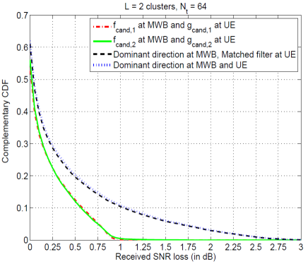
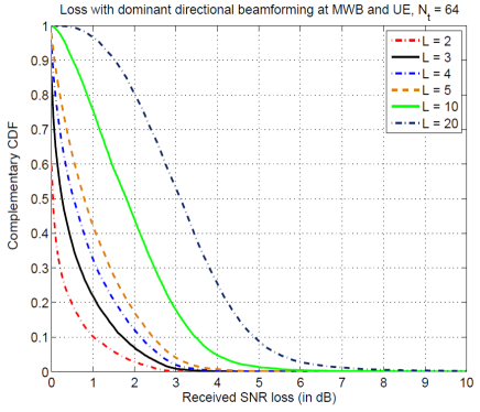
(a)	(b)

Figure 1: Complementary CDF of loss in ${\sf SNR}_{\sf rx}$ between the optimal beamforming scheme from ${\cal F}_{2}^{N_{t}}$ in (7) relative to: (a) different beamforming solutions with $L=2$ clusters, and (b) a dominant directional beamforming scheme with different choices of $L$.

III-C Issues with RSV Learning

The (near-)optimality of the RSV-type solutions from ${\cal F}_{2}^{N_{t}}$ and ${\cal F}_{\infty}^{N_{t}}$ suggests that a reasonable approach for beamformer design is to let the MWB and UE learn an approximation to ${\bf f}_{\sf opt}$ and ${\bf g}_{\sf opt}$, respectively. A similar approach is adopted at cellular frequencies under the rubric of limited feedback schemes that approximate the RSV of the channel from a codebook of beamforming vectors. We specialize this approach and elaborate on their appropriateness for mmW systems.

A well-known RSV learning scheme that exploits the time division duplexing(TDD)-reciprocity of the channel ${\sf H}$ is power iteration [45, Sec. 7.3] which iterates ($i=0,1,\cdots$) a randomly initialized beamforming vector (${\bf f}_{0}$) over the channel as follows:

$$\widetilde{\bf g}_{i+1} = \sqrt{\rho_{\sf f}}\cdot{\sf H}{\bf f}_{i}+{\bf n}_{{\sf f},\hskip 1.4457pti+1}$$ (22)

$${\bf g}_{i+1} = \frac{\widetilde{\bf g}_{i+1}}{\|\widetilde{\bf g}_{i+1}\|_{2}}=\frac{\sqrt{\rho_{\sf f}}\cdot{\sf H}{\bf f}_{i}+{\bf n}_{{\sf f},\hskip 1.4457pti+1}}{\|\sqrt{\rho_{\sf f}}\cdot{\sf H}{\bf f}_{i}+{\bf n}_{{\sf f},\hskip 1.4457pti+1}\|_{2}}$$ (23)

$${\bf z}_{i+1} = \sqrt{\rho_{\sf r}}\cdot{\sf H}^{T}{\bf g}_{i+1}^{\star}+{\bf n}_{{\sf r},\hskip 1.4457pti+1}^{\star}$$ (24)

$${\bf f}_{i+1} = \frac{{\bf z}_{i+1}^{\star}}{\|{\bf z}_{i+1}\|_{2}}=\frac{\sqrt{\rho_{\sf r}}\cdot{\sf H}^{H}{\bf g}_{i+1}+{\bf n}_{{\sf r},\hskip 1.4457pti+1}}{\|\sqrt{\rho_{\sf r}}\cdot{\sf H}^{H}{\bf g}_{i+1}+{\bf n}_{{\sf r},\hskip 1.4457pti+1}\|_{2}}.$$ (25)

In (22)-(25), $\rho_{\sf f}$ and $\rho_{\sf r}$ stand for the pre-beamforming ${\sf SNR}$s of the forward and reverse links, respectively. A straightforward simplification shows that

$${\bf f}_{i+1}=\frac{\sqrt{\rho_{\sf f}\rho_{\sf r}}\cdot{\sf H}^{H}{\sf H}\hskip 1.4457pt{\bf f}_{i}+\sqrt{\rho_{\sf r}}\hskip 1.4457pt{\sf H}^{H}{\bf n}_{{\sf f},\hskip 1.4457pti+1}+\|\sqrt{\rho_{\sf f}}\hskip 1.4457pt{\sf H}\hskip 1.4457pt{\bf f}_{i}+{\bf n}_{{\sf f},\hskip 1.4457pti+1}\|_{2}\cdot{\bf n}_{{\sf r},\hskip 1.4457pti+1}}{\|\sqrt{\rho_{\sf f}\rho_{\sf r}}\cdot{\sf H}^{H}{\sf H}\hskip 1.4457pt{\bf f}_{i}+\sqrt{\rho_{\sf r}}\hskip 1.4457pt{\sf H}^{H}{\bf n}_{{\sf f},\hskip 1.4457pti+1}+\|\sqrt{\rho_{\sf f}}\hskip 1.4457pt{\sf H}\hskip 1.4457pt{\bf f}_{i}+{\bf n}_{{\sf f},\hskip 1.4457pti+1}\|_{2}\cdot{\bf n}_{{\sf r},\hskip 1.4457pti+1}\|_{2}}.$$ (26)

When the system is noise-free ($\{\rho_{\sf f},\hskip 1.4457pt\rho_{\sf r}\}\rightarrow\infty$), the above algorithm reduces to

$${\bf f}_{i+1} \rightarrow \frac{{\sf H}^{H}{\sf H}\hskip 1.4457pt{\bf f}_{i}}{\|{\sf H}^{H}{\sf H}\hskip 1.4457pt{\bf f}_{i}\|_{2}}\Longrightarrow{\bf f}_{i+1}\rightarrow\frac{\left({\sf H}^{H}{\sf H}\right)^{i+1}{\bf f}_{0}}{\|\left({\sf H}^{H}{\sf H}\right)^{i+1}{\bf f}_{0}\|_{2}}$$ (27)

$${\bf g}_{i+1} \rightarrow \frac{{\sf H}\hskip 1.4457pt{\bf f}_{i}}{\|{\sf H}\hskip 1.4457pt{\bf f}_{i}\|_{2}}\Longrightarrow{\bf g}_{i+1}\rightarrow\frac{{\sf H}\left({\sf H}^{H}{\sf H}\right)^{i+1}{\bf f}_{0}}{\|{\sf H}\left({\sf H}^{H}{\sf H}\right)^{i+1}{\bf f}_{0}\|_{2}}.$$ (28)

With ${\sf H}^{H}{\sf H}={\sf V}{\sf\Lambda}{\sf V}^{H}$, we have

$${\bf f}_{i+1}=\frac{\sum_{j=1}^{N_{t}}{\sf v}_{j}\cdot\left({\sf v}_{j}^{H}{\bf f}_{0}\right)\cdot\left({\sf\Lambda}_{j}\right)^{i+1}}{\|\sum_{j=1}^{N_{t}}{\sf v}_{j}\cdot\left({\sf v}_{j}^{H}{\bf f}_{0}\right)\cdot\left({\sf\Lambda}_{j}\right)^{i+1}\|_{2}}.$$ (29)

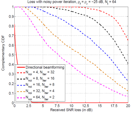
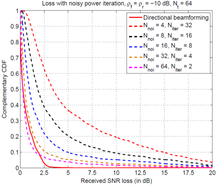
(a)	(b)

Figure 2: Complementary CDF of loss in ${\sf SNR}_{\sf rx}$ between the optimal beamforming scheme from ${\cal F}_{2}^{N_{t}}$ in (7) and the noisy power iteration scheme with (a) $\rho_{\sf f}=\rho_{\sf r}=-25$ dB and (b) $\rho_{\sf f}=\rho_{\sf r}=-10$ dB.

While the noise-free power iteration scheme has been proposed in the MIMO context in [26], understanding the performance tradeoff of the noisy case analytically appears to be a difficult problem, in general. To surmount this difficulty, we numerically study the performance of the noisy case at a low pre-beamforming ${\sf SNR}$ on the order of $-25$ to $-10$ dB. We consider the case where $N_{\sf npi}=256$ samples are used for RSV learning and these samples are partitioned in different ways as $N_{\sf npi}=2N_{\sf noi}\times N_{\sf iter}$. Here, $N_{\sf noi}$ samples are used to improve $\rho_{\sf f}$ by noise averaging and $N_{\sf iter}$ samples are used for beamformer iteration. In particular, we consider the following choices for $N_{\sf noi}$ in our study: $\{4,8,16,32,64\}$ with $\rho_{\sf f}=\rho_{\sf r}=\{-25,\hskip 1.4457pt-10\}$ dB and Figs. 2(a)-(b) plot the complementary cumulative distribution function (CDF) of the loss in ${\sf SNR}_{\sf rx}$ for these two scenarios in a $L=2,N_{r}=4$ and $N_{t}=64$ system with averaging over the random choice of ${\bf f}_{0}$. From these two plots, we observe that given $N_{\sf npi}$ samples, noise averaging is a task of higher importance at low pre-beamforming ${\sf SNR}$s than beamformer iteration. Nevertheless, in spite of the best noise averaging, the noisy power iteration scheme has a poor performance at low ${\sf SNR}$s (for a large fraction of the users at $-25$ dB and a good fraction at $-10$ dB) as noise is amplified in the iteration process rather than the channel’s RSV.

The RSV learning scheme also suffers from other problems that make its applicability in mmW systems difficult. Since each user’s RSV has to be learned via a bi-directional iteration, it is not amenable (in this form) as a common broadcast solution for the downlink setting. This is particularly disadvantageous and impractical if each MWB has to initiate a unicast session with a UE that is yet to be discovered. Further, the need to sample each antenna individually (at both ends) can considerably slow down the iteration process with RF hardware constraints (e.g., when there are fewer RF chains than antennas). In addition, this approach requires calibration of the receive-side RF chain relative to the transmit-side RF chain with respect to phase and amplitude as well as phase coherence during the iteration. More importantly, this approach critically depends on TDD reciprocity, which could be complicated in certain deployment scenarios that do not allow this possibility [9].

An alternate approach given the RSV structure in Theorem 1 is to learn the dominant directions at the MWB end $\{\widehat{\phi}_{{\sf T},\ell}\}$ and then combine the beams with appropriate weights $\{\widehat{\alpha}_{\ell}\}$ to result in a beamforming vector:

$${\bf f}_{\sf comb}=\frac{\sum_{\ell=1}^{L}\widehat{\alpha}_{\ell}\hskip 3.61371pt{\sf CPO}(\widehat{\phi}_{{\sf T},\ell})}{\|\sum_{\ell=1}^{L}\widehat{\alpha}_{\ell}\hskip 3.61371pt{\sf CPO}(\widehat{\phi}_{{\sf T},\ell})\|_{2}}.$$ (30)

The difficulty with this approach is that it suffers from PA inefficiency (not all the PAs operate at maximal power). Fig. 3(a) plots the complementary CDF of the peak-to-average ratio (PAR) of ${\bf f}_{\sf comb}$, defined as,

$${\sf PAR}\triangleq\frac{\max_{i}|{\bf f}_{\sf comb}(i)|^{2}}{1/N_{t}}=N_{t}\cdot\max_{i}|{\bf f}_{\sf comb}(i)|^{2}$$ (31)

corresponding to beam combining along two randomly chosen, but known directions with random weights. Fig. 3(a) shows that a median PAR loss of over $2$ dB is seen for $N_{t}\geq 8$ suggesting that the RSV gain relative to directional beamforming of less than a dB (see Fig. 1(a)) is significantly outweighed by the PA inefficiency. In other words, the ${\sf SNR}_{\sf rx}$ loss with just selecting the dominant direction at the MWB and the UE ends is far less than the PA backoff due to combining multiple directions at the MWB or the UE.

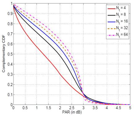
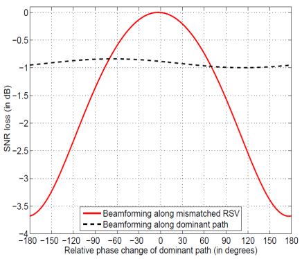
(a)	(b)

Figure 3: (a) Complementary CDF of PAR of the combined beamforming vector needed to mimic the RSV structure. (b) Typical performance loss with mismatched RSV and mismatched dominant directional beamforming schemes relative to optimal beamforming in the perturbed case.

More generally, any RSV learning scheme is bound to be extremely sensitive to relative phase changes across paths. For example, Fig. 3(b) plots the typical behavior of loss in ${\sf SNR}_{\sf rx}$ with the mismatched reuse of the optimal beamformer and the dominant directional beamformer (both from the unperturbed case) relative to the optimal beamformer in the perturbed case as the phase of the dominant path in a $L=2,N_{r}=4,N_{t}=64$ system changes. In this example, the two paths are such that $\phi_{{\sf R},1}=108.57^{\sf o}$, $\phi_{{\sf T},1}=83.74^{\sf o}$, $\alpha_{1}=2.61$, $\phi_{{\sf R},2}=92.74^{\sf o}$, $\phi_{{\sf T},2}=94.26^{\sf o}$, $\alpha_{2}=1.79$. We note that the RSV scheme takes a steep fall in performance as the phase changes, whereas the directional scheme remains approximately stable in performance. It is important to note that a $360^{\sf o}$ change in phase corresponds to a change in path length of $\lambda$ (a small distance at higher carrier frequencies and hence an increasingly likely possibility). Such a sensitivity for any RSV reconstruction scheme to phase changes renders this approach’s utility in the mmW context questionable.

IV Directional Beamforming and Direction Learning

Instead of the RSV solution, we now consider the performance loss with a low-complexity strategy that beamforms along the dominant direction at the MWB and the UE. From the numerical study in Fig. 1(a), we see that the dominant directional beamforming scheme suffers only a minimal loss relative to even the best scheme from ${\cal F}_{2}^{N_{t}}$ and ${\cal F}_{2}^{N_{r}}$ (a median loss of a fraction of a dB and less than a dB even at the $90$-th percentile level). Further, Fig. 1(b) plots the complementary CDF of the loss in ${\sf SNR}_{\sf rx}$ between the optimal scheme in (7) and the dominant directional beamforming scheme with different choices of $L$: $L=2,3,4,5,10$ or $20$. From this study, we note that directional beamforming results in less than a dB loss for over $50\%$ of the users for even up to $L=5$ clusters. Further, directional beamforming results in no more than $2.5$ dB loss for even up to $90\%$ of the users. Thus, this study suggests that learning the directions (AoAs/AoDs) along which the UE and MWB should beamform is a useful strategy for initial UE discovery.

IV-A Learning Dominant Directions via Subspace Methods

AoA/AoD learning with multiple antenna arrays has a long and illustrious history in the signal/array processing literature [30]. In the simplest case of estimating a single unknown source (signal direction) at the UE end with system equation:

$${\bf y}=\alpha_{1}{\bf u}(\phi_{1})+{\bf n}$$ (32)

where $\alpha_{1}$ is known, ${\bf u}(\cdot)$ denotes the array steering vector and ${\bf n}\sim{\cal CN}({\bf 0},{\bf I})$, it can be seen that the density function $\log\left(f({\bf y}|\alpha_{1},\phi_{1})\right)$ can be written as ${\sf C}-({\bf y}-\alpha_{1}{\bf u}(\phi_{1}))^{H}({\bf y}-\alpha_{1}{\bf u}(\phi_{1}))$ for an appropriately defined constant ${\sf C}$. Thus, the maximum likelihood (ML) solution ($\widehat{\phi}_{1}$) that maximizes the density can be seen to be $\widehat{\phi}_{1}=\arg\max_{\phi}|{\bf u}(\phi)^{H}{\bf y}|^{2}$. Rephrasing, correlation of the received vector ${\bf y}$ for the best signal strength results in the ML solution for the problem of signal coming from one unknown direction.

In general, if there are multiple ($K$) sources with system equation

$${\bf y}=\sum_{k=1}^{K}\alpha_{k}{\bf u}(\phi_{k})+{\bf n},$$ (33)

the density function of ${\bf y}$ is non-convex in the parameters resulting in a numerical multi-dimensional search in the parameter space. In this context, the main premise behind the MUSIC algorithm [28] is that the signal subspace is $K$-dimensional and is orthogonal to the noise subspace. Furthermore, the $K$ largest eigenvalues of the estimated received covariance matrix, $\widehat{\bf R}_{\bf y}$, correspond to the signal subspace and the other eigenvalues to the noise subspace (provided the covariance matrix estimate is reliable). The MUSIC algorithm then estimates the signal directions by finding the ($K$) peaks of the pseudospectrum, defined as,

$$P_{\sf MUSIC}(\phi)\triangleq\frac{1}{\sum_{n=K+1}^{N_{r}}|{\bf u}(\phi)^{H}\widehat{\bf q}_{n}|^{2}}$$ (34)

where $\{\widehat{\bf q}_{K+1},\cdots,\widehat{\bf q}_{N_{r}}\}$ denote the eigenvectors of the noise subspace of $\widehat{\bf R}_{\bf y}$. The principal advantage of the MUSIC algorithm is that the signal maximization task has been recasted as a noise minimization task, a one-dimensional line search problem albeit at the cost of computing the eigenvectors of $\widehat{\bf R}_{\bf y}$. Nevertheless, since $\{\widehat{\bf q}_{1},\cdots,\widehat{\bf q}_{N_{r}}\}$ can be chosen to form a unitary basis, it is seen that MUSIC attempts to maximize $\sum_{n=1}^{K}|{\bf u}(\phi)^{H}\widehat{\bf q}_{n}|^{2}$ (or in other words, it assigns equal weights to all the components of the signal subspace and is hence not ML-optimal).

We now apply the MUSIC algorithm to direction learning at the MWB and UE by a bi-directional approach where the MWB learns the AoD by estimating the uplink covariance matrix (where the UE trains the MWB), and the UE learns the AoA by estimating the downlink covariance matrix (where the MWB trains the UE). We consider the case where $N_{\sf music}=256$ samples are used for direction learning. Since the MWB is equipped with more antennas than the UE, we partition $N_{\sf music}$ into $N_{\sf up}=192$ samples for uplink (AoD) training and $N_{\sf down}=64$ samples for downlink (AoA) training. As before, we partition $N_{\sf up}$ in different ways as $N_{\sf up}=N_{\sf up,cov}\times N_{\sf up,noi}$ where $N_{\sf up,noi}$ samples are used for link margin improvement and $N_{\sf up,cov}$ samples are used for uplink covariance matrix estimation. In particular, we study the following choices here: $N_{\sf up,cov}=\{12,24,32,48,64,96\}$. $N_{\sf down}=64$ is partitioned as $N_{\sf down,noi}=N_{\sf down,cov}=8$. Figs. 4(a) and (b) plot the complementary CDF of ${\sf SNR}_{\sf rx}$ with such a bi-directional MUSIC algorithm for $\rho_{\sf f}=\rho_{\sf r}=-25$ dB and $-10$ dB, respectively. In general, $\rho_{\sf f}>\rho_{\sf r}$ and Fig. 4 serves as a more optimistic characterization of the MUSIC scheme for mmW systems.

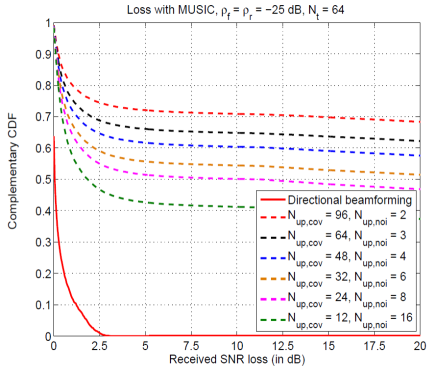
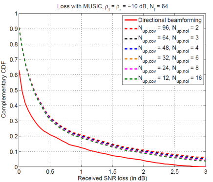
(a)	(b)

Figure 4: Complementary CDF of loss in ${\sf SNR}_{\sf rx}$ between the optimal beamforming scheme in ${\cal F}_{2}^{N_{t}}$ in (7) and MUSIC with (a) $\rho_{\sf f}=\rho_{\sf r}=-25$ dB and (b) $\rho_{\sf f}=\rho_{\sf r}=-10$ dB.

From Fig. 4, we note that the performance is rather poor at low link margins, but significantly better as the link margin improves. An important reason for the poor performance of the MUSIC approach is that consistent covariance matrix estimation becomes a difficult exercise with very few samples, especially as the antenna dimensions increase at the MWB end. Furthermore, as with the noisy power iteration scheme, MUSIC also requires a non-broadcast system design. It also suffers from a high computational complexity (dominated by the eigen-decomposition of an $N_{t}\times N_{t}$ matrix in uplink training). In general, the computational complexity of MUSIC can be traded off by constraining the antenna array structure in various ways. Nevertheless, we expect the computational complexity of other such constrained AoA/AoD learning techniques such as Estimation of Signal Parameters via Rotational Invariance Techniques (ESPRIT) algorithm [29], Space-Alternating Generalized Expectation maximization (SAGE) algorithm [49, 50], higher-order singular value decomposition, RIMAX [51], and compressive sensing techniques that employ nuclear norm optimization [52, 53, 54] to be of similar nature as the MUSIC algorithm. All these reasons suggest that while the MUSIC algorithm may be useful for beam refinement after the UE has been discovered, its utility in UE discovery is questionable.

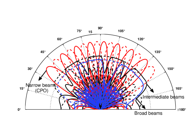
Figure 5: Main idea of beam broadening illustrated with the overlaid beam patterns of beamforming vectors from three (narrow/${\sf CPO}$ beams, intermediate beams and broad beams) codebooks.

IV-B Beam Broadening for Initial UE Discovery

Let $\Omega$ denote the beamspace transformation at the MWB side, $\Omega=kd_{\sf T}\cos(\phi_{\sf T})=\pi\cos(\phi_{\sf T})$, corresponding to an inter-antenna spacing of $\lambda/2$. Towards the goal of alternate direction learning strategies, we consider the problem of understanding the tradeoff in the design of beamforming vectors that cover a beamspace area of $\overline{\Omega}$ with as few beamforming vectors as possible without sacrificing the worst-case beamforming gain in the coverage area [15, 34].

The basic idea of beam broadening is illustrated in Fig. 5 where three different codebooks of beamforming vectors are used to cover a coverage area of $120^{\sf o}$ (from $30^{\sf o}$ to $150^{\sf o}$). The first codebook (illustrated in red) consists of narrow ${\sf CPO}$ beams (pointing at optimally chosen directions over the coverage area) which leads to a peak beamforming gain of $10\log_{10}(N_{t})$ dB as well as a reasonably high worst-case beamforming gain over the coverage area, although at the cost of a high UE discovery latency corresponding to a beam sweep over $16$ directions/beams. The second codebook (illustrated in black) consists of intermediate beams which leads to a lower peak beamforming gain (as well as a worst-case gain) over the coverage area, but the UE discovery period is shortened as it now consists of a beam sweep over $8$ directions/beams. The third codebook (illustrated in blue) consists of broad beams which leads to a more reduced peak beamforming gain, but the UE discovery period is a sweep over only $4$ directions/beams. Either codebook could be useful for initial UE discovery depending on the link margin of the UE’s involved. For example, a UE geographically close to the MWB and suffering minimal path loss can accommodate a broad beam codebook and be quickly discovered, whereas a UE at the cell-edge or suffering from huge blocking losses may need the narrow ${\sf CPO}$ beam codebook to even close the link with the MWB. The intermediate codebook trades off these two properties.

We now recast the above idea in the form of a well-posed optimization problem. For this, given a beamspace coverage area of $\Omega_{0}$ for a single beam (centered around $\Omega_{\sf c}=\pi/2$, without loss in generality), we seek the design of:

$${\bf f}_{\Omega_{0}}\triangleq\arg\max\limits_{{\bf f}\hskip 1.4457pt\in\hskip 1.4457pt{\cal F}_{\infty}^{N_{t}}}\min\limits_{\Omega\hskip 1.4457pt\in\hskip 1.4457pt\left[\Omega_{\sf c}-\frac{\Omega_{0}}{2},\hskip 1.4457pt\Omega_{\sf c}+\frac{\Omega_{0}}{2}\right]}|{\bf F}(\Omega)|^{2}$$ (35)

where ${\bf F}(\Omega)=\sum_{n=0}^{N_{t}-1}{\bf f}(n)e^{-j\Omega n}={\bf a}(\Omega)^{H}{\bf f}$ with ${\bf a}(\Omega)=\left[1,\hskip 1.4457pte^{j\Omega},\cdots,e^{j(N_{t}-1)\Omega}\right]^{T}$. With ${\bf f}_{\Omega_{0}}$ as template, the number of beamforming vectors needed to cover $\overline{\Omega}$ (say, a $120^{\sf o}$ field-of-view as in Fig. 5) is ${\sf No.\hskip 1.4457ptbeams}=\frac{\overline{\Omega}}{\Omega_{0}}$.

We start with an upper bound on the tradeoff between ${\sf No.\hskip 1.4457ptbeams}$ and the worst-case beamforming gain over $\overline{\Omega}$. From the Parseval identity, we have the following trivial relationship for any ${\bf f}$:

$$\frac{1}{2\pi}\int_{-\pi}^{\pi}|{\bf F}(\Omega)|^{2}d\Omega=\sum_{n=0}^{N_{t}-1}|{\bf f}(n)|^{2}\leq 1.$$ (36)

If $\min\limits_{\Omega\hskip 1.4457pt\in\hskip 1.4457pt\left[\Omega_{\sf c}-\frac{\Omega_{0}}{2},\hskip 1.4457pt\Omega_{\sf c}+\frac{\Omega_{0}}{2}\right]}|{\bf F}(\Omega)|^{2}=P$, we have

$$\frac{1}{2\pi}\int_{-\pi}^{\pi}|{\bf F}(\Omega)|^{2}d\Omega\geq\frac{1}{2\pi}\int_{\Omega\hskip 1.4457pt\in\hskip 1.4457pt\left[\Omega_{\sf c}-\frac{\Omega_{0}}{2},\hskip 1.4457pt\Omega_{\sf c}+\frac{\Omega_{0}}{2}\right]}|{\bf F}(\Omega)|^{2}d\Omega\geq P\cdot\frac{\Omega_{0}}{2\pi}\Longrightarrow P\leq\frac{2\pi}{\Omega_{0}}.$$ (37)

Further, $P$ is also constrained as $P\leq N_{t}$ since the maximal beamforming gain cannot exceed $N_{t}$ in any direction. Thus, the worst-case beamforming gain over this area (in dB) is upper bounded as

$${\sf BF\hskip 3.61371ptGain} \triangleq 10\log_{10}\left(P\right)\leq 10\log_{10}\left(\min\left(N_{t},\hskip 1.4457pt\frac{2\pi}{\overline{\Omega}}\cdot{\sf No.\hskip 1.4457ptbeams}\right)\right).$$ (38)

We now provide an alternate non-trivial approach based on computation of eigenvalues of certain appropriately-defined matrices for a better upper bound of this tradeoff.

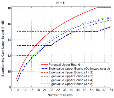
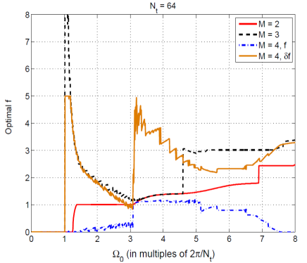
(a)	(b)
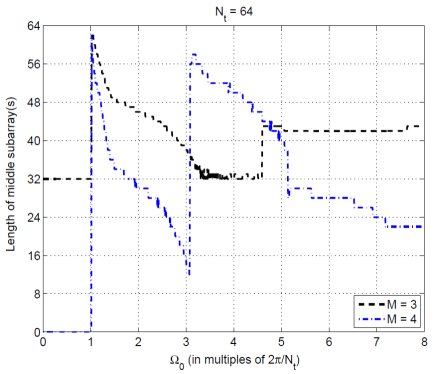
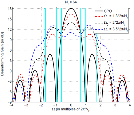
(c)	(d)

Figure 6: (a) Upper bound to the beamforming gain vs. number of beams tradeoff for $N_{t}=64$. (b) Optimal ${\sf f}$ and (c) length of middle subarray(s) as a function of $\Omega_{0}$ for different choices of $M$. (d) Beam patterns of broadened beams for certain choices of $\Omega_{0}$ in the $M=2$ case.

Theorem 3.

Let $\Omega_{j},\hskip 3.61371ptj=1,\cdots,J$ be a set of sampling frequencies over the beamspace area of $\Omega_{0}$ spanned by the beamforming vector ${\bf f}$. The worst-case beamforming gain with ${\bf f}$ is upper bounded by the solution to the following optimization:

$${\sf BF\hskip 3.61371ptGain}\leq 10\log_{10}\left(N_{t},\hskip 3.61371pt\min\limits_{J,\hskip 1.4457pt\{\Omega_{j}\}}\frac{\lambda_{\sf max}\left(\sum_{j=1}^{J}{\bf a}(\Omega_{j}){\bf a}(\Omega_{j})^{H}\right)}{J}\right)$$ (39)

where $\Omega_{j}\in\left[\Omega_{\sf c}-\frac{\Omega_{0}}{2},\hskip 1.4457pt\Omega_{\sf c}+\frac{\Omega_{0}}{2}\right]$ with $\Omega_{0}=\frac{\overline{\Omega}}{{\sf No.\hskip 1.4457ptbeams}}$ and $\lambda_{\sf max}(\bullet)$ stands for the largest eigenvalue of the underlying positive semi-definite matrix.

Proof.

See Appendix -D. ∎

Fig. 6(a) numerically optimizes the expression in (39) and plots the upper bound to the worst-case beamforming gain as a function of the number of beams to cover a $120^{\sf o}$ field-of-view with $N_{t}=64$. For the eigenvalue-based approach, we plot the upper bound for specific choices of $J$ with $\{\Omega_{j}\}$ optimized, as well as the upper bound based on a joint optimization over $J$ and $\{\Omega_{j}\}$. Note that the horizontal segments in the joint optimization correspond to the fact that the tradeoff with a larger number of beams can be no worser than the tradeoff with a smaller number of beams.

In contrast to the upper bound, we now propose specific approaches towards the goal of beam broadening. For this, we initially consider partitioning of the antenna array at the MWB side into virtual subarrays where each virtual subarray is used to beamform to a certain appropriately-chosen virtual direction. The expectation from this approach is that the beam patterns from the individual virtual subarrays combine to enhance the coverage area of the resultant beam with minimal loss in peak gain due to reduction in the effective aperture of the subarrays.

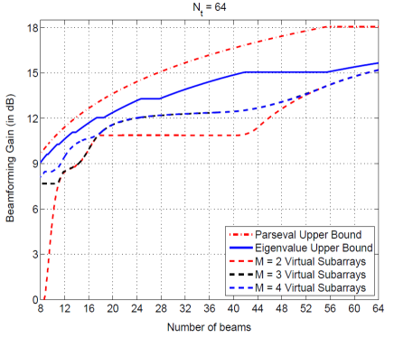
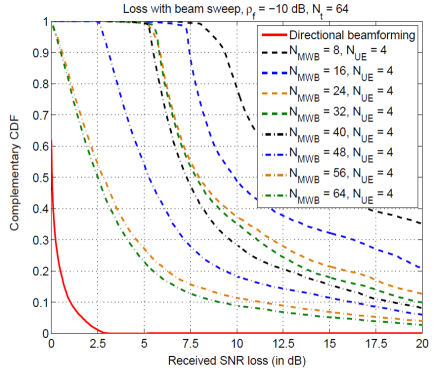
(a)	(b)

Figure 7: (a) Performance tradeoff with different beam broadening approaches for $N_{t}=64$. (b) Complementary CDF of loss in ${\sf SNR}_{\sf rx}$ between the optimal beamforming scheme in ${\cal F}_{2}^{N_{t}}$ in (7) and beam sweep with the broadened beams as in Fig. 7(a) at $\rho_{\sf f}=-10$ dB.

As a specific example, in the $M=2$ virtual subarray setting, we propose the following beamforming vector that orients along $\pi-\cos^{-1}\left(\frac{2{\sf f}}{N_{t}}\right)$ and $\cos^{-1}\left(\frac{2{\sf f}}{N_{t}}\right)$ with each half of the array. That is,

$${\bf f}(n)=\frac{1}{\sqrt{N_{t}}}\left\{\begin{array}[]{ll}\exp\left(-\frac{j2\pi{\sf f}}{N_{t}}(n-\frac{N_{t}}{2}+\frac{1}{2})\right)&{\sf if}\hskip 3.61371pt0\leq n\leq\frac{N_{t}}{2}-1\\ \exp\left(\frac{j2\pi{\sf f}}{N_{t}}(n-\frac{N_{t}}{2}+\frac{1}{2})\right)&{\sf if}\hskip 3.61371pt\frac{N_{t}}{2}\leq n\leq N_{t}-1\end{array}\right.$$ (42)

where ${\bf f}$ is designed to be a broadened beam by optimally choosing ${\sf f}$. Similarly, in the $M=3$ and $M=4$ settings, we propose the following beamforming vectors with two parameters (${\sf f}$ and $0\leq L\leq\frac{N_{t}}{2}$) and three parameters (${\sf f}$,   $\delta{\sf f}$ and $0\leq L\leq\frac{N_{t}}{2}$), respectively:

$${\bf f} = \frac{1}{\sqrt{N_{t}}}\left\{\begin{array}[]{ll}\exp\left(-\frac{j2\pi{\sf f}}{N_{t}}(n-\frac{N_{t}}{2}+\frac{1}{2}+L)\right)&{\sf if}\hskip 3.61371pt0\leq n\leq\frac{N_{t}}{2}-L-1\\ 1&{\sf if}\hskip 3.61371pt\frac{N_{t}}{2}-L\leq n\leq\frac{N_{t}}{2}+L-1\\ \exp\left(\frac{j2\pi{\sf f}}{N_{t}}(n-\frac{N_{t}}{2}+\frac{1}{2}-L)\right)&{\sf if}\hskip 3.61371pt\frac{N_{t}}{2}+L\leq n\leq N_{t}-1,\end{array}\right.$$ (46)

$${\bf f} = \frac{1}{\sqrt{N_{t}}}\left\{\begin{array}[]{ll}\exp\left(-\frac{j2\pi({\sf f}+\delta{\sf f})}{N_{t}}(n-\frac{N_{t}}{2}+\frac{1}{2})-\frac{j2\pi\cdot\delta{\sf f}}{N_{t}}\left(L-\frac{1}{2}\right)\right)&{\sf if}\hskip 3.61371pt0\leq n\leq\frac{N_{t}}{2}-L-1\\ \exp\left(-\frac{j2\pi{\sf f}}{N_{t}}(n-\frac{N_{t}}{2}+\frac{1}{2})\right)&{\sf if}\hskip 3.61371pt\frac{N_{t}}{2}-L\leq n\leq\frac{N_{t}}{2}-1\\ \exp\left(\frac{j2\pi{\sf f}}{N_{t}}(n-\frac{N_{t}}{2}+\frac{1}{2})\right)&{\sf if}\hskip 3.61371pt\frac{N_{t}}{2}\leq n\leq\frac{N_{t}}{2}+L-1\\ \exp\left(\frac{j2\pi({\sf f}+\delta{\sf f})}{N_{t}}(n-\frac{N_{t}}{2}+\frac{1}{2})-\frac{j2\pi\cdot\delta{\sf f}}{N_{t}}\left(L-\frac{1}{2}\right)\right)&{\sf if}\hskip 3.61371pt\frac{N_{t}}{2}+L\leq n\leq N_{t}-1.\end{array}\right.$$ (51)

Note that (46) reduces to the $M=2$ setting in (42) with $L=0$ where the beams are pointed at ${\sf f}$, and with $L=\frac{N_{t}}{2}$ where the beams are pointed at ${\sf f}=0$. Similarly, (51) reduces to the $M=2$ setting with $L=0$ and $L=\frac{N_{t}}{2}$ where the beams are pointed at ${\sf f}+\delta{\sf f}$ and ${\sf f}$, respectively.

Fig. 6(b) plots the optimal values of ${\sf f}$ (and $\delta{\sf f}$) designed to maximize $\min|{\bf F}(\Omega)|^{2}$ as a function of $\Omega_{0}$ with $M=2,3,4$ and $N_{t}=64$. Fig. 6(c) plots the length of the middle subarray in the $M=3$ case (middle subarrays in the $M=4$ case) as a function of $\Omega_{0}$. From these two plots, we see that for small values of $\Omega_{0}$, choosing ${\sf f}=0$ is optimal, whereas the length of the middle subarray decreases as $\Omega_{0}$ increases corresponding to gradual beam orientation away from ${\sf f}=0$. Fig. 6(d) plots the shape of the broadened beams so optimized for three choices of $\Omega_{0}$: $\frac{\Omega_{0}}{2\pi/N_{t}}=\{1.3,\hskip 3.61371pt2,\hskip 3.61371pt3.5\}$. Also, plotted are vertical lines at $\frac{\Omega_{0}}{2\pi/N_{t}}=\pm 1.3,\hskip 3.61371pt\pm 2,\hskip 3.61371pt\pm 3.5$. From this plot, we see that within their corresponding regimes, each broadened beam maximizes $\min|{\bf F}(\Omega)|^{2}$. In addition, Fig. 7(a) captures the tradeoff between the number of beamforming vectors and the worst-case beamforming gain with the $M=2,3,4$ subarray scheme in the $N_{t}=64$ case. Clearly, across all regimes of interest of ${\sf No.\hskip 3.61371ptbeams}$, the $M=4$ subarray scheme is within a couple of dB of the upper bound in terms of beamforming gain illustrating the utility of the proposed approach.

IV-C Learning Dominant Directions via Beam Sweep with Broadened Beam Codebooks

We use the template broadened beamforming vectors designed in Sec. IV-B corresponding to different beam broadening factors (and their shifted versions) to design a beam sweep codebook for the MWB side. In particular, we consider those beam broadening factors that lead to $N_{\sf mwb}=\{8,\hskip 3.61371pt16,\hskip 3.61371pt24,\hskip 3.61371pt32,\hskip 3.61371pt40,\hskip 3.61371pt48,\hskip 3.61371pt56,\hskip 3.61371pt64\}$ elements in the beam sweep codebook at the MWB. On the other hand, since $N_{r}=4$ at the UE side, a simpler codebook of $N_{\sf ue}=4$ beamforming vectors corresponding to an equal partition of the field-of-view is sufficient for the purpose of beam sweep. With these different codebook choices at the MWB and UE, we find the best choice of beamforming vectors that maximize ${\sf SNR}_{\sf rx}$ and use them for subsequent beamforming/beam refinement. An important advantage of the beam sweep approach is that it allows a broadcast solution (the same codebook can be reused across multiple UEs within the field-of-view).

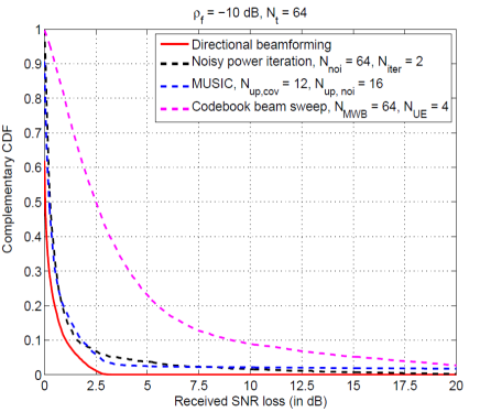
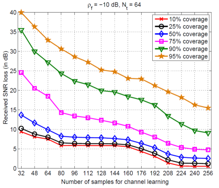
(a)	(b)

Figure 8: (a) Comparison of complementary CDF of ${\sf SNR}_{\sf rx}$ loss with different beamforming approaches at $\rho_{\sf f}=\rho_{\sf r}=-10$ dB. (b) Tradeoff between number of samples for channel learning with the beam sweep approach and loss in ${\sf SNR}_{\sf rx}$ in initial UE discovery.

Fig. 7(b) plots the complementary CDF of the loss in ${\sf SNR}_{\sf rx}$ with the beam sweep approach at $\rho_{\sf f}=-10$ dB. Fig. 8(a) compares the complementary CDF of loss in ${\sf SNR}_{\sf rx}$ with the best noisy power iteration scheme, MUSIC algorithm and the beam sweep approach at the same $\rho_{\sf f}$ value. Clearly, the beam sweep approach has a poorer performance relative to the other schemes, but its simplicity results in a better system design than possible with the other approaches. Further, Fig. 8(b) plots the loss in ${\sf SNR}_{\sf rx}$ at different percentile levels ($10\%,\hskip 1.4457pt25\%,\hskip 1.4457pt50\%,\hskip 1.4457pt75\%,\hskip 1.4457pt90\%$ and $95\%$) as a function of the number of samples used in channel learning with the beam sweep scheme. From this study, we note that at small coverage levels, certain codebook size choices are better in the tradeoff curve than other choices (for example, a $N_{\sf mwb}=20$ codebook over a $N_{\sf mwb}=40$ codebook) and these advantages correspond to the steepness of the achievability curve (see Fig. 7(a)).

Further, while ${\sf SNR}_{\sf rx}$ improves as the codebook size increases, good users with a better link margin (e.g., users with a smaller path loss) can be discovered with a lower discovery latency (corresponding to a smaller codebook size) than those cell-edge/blocked users with a worser link margin. Fig. 8(b) suggests a smooth roll-off in the discovery latency of the users with a worser link margin. That said, the beam sweep approach could indeed suffer a significant loss in performance especially with a cell-edge/blocked user. In such scenarios, the design for such a user could include coding over long sequences for enhanced time-repetition/processing gain, high MWB densification, a low-frequency overlay of multiple narrow CPO beams with a worst-case beamforming gain (as close to the $10\log_{10}(N_{t})$ dB peak gain) in the coverage area, among many approaches. However, such a design could lead to a significant drag on the performance tradeoffs of the good/median user. Thus, they could be initiated by the UE when it perceives a poor link on a unicast basis.

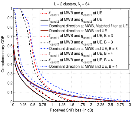
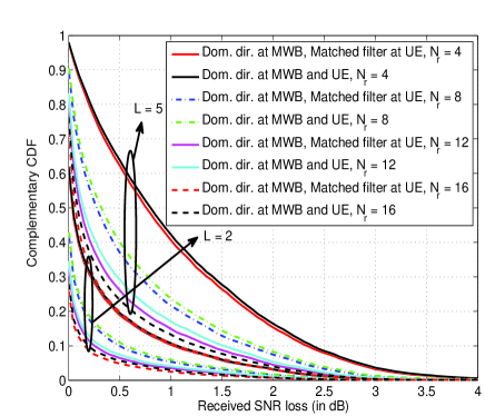
(a)	(b)

Figure 9: (a) Loss in ${\sf SNR}_{\sf rx}$ with different RSV-type beamforming schemes with perfect phase of beamformers, and finite $B=3$ and $B=4$ bit phase quantization. (b) Complementary CDF of loss in ${\sf SNR}_{\sf rx}$ as a function of $N_{r}$ with $L=2$ and $L=5$ clusters.

V Comments on Practical Applications

V-A Finite-Bit Phase Shifters

The entire focus of this work has been on beamformers that can be realized with infinite-precision phase shifters allowing an arbitrary phase resolution for the beamformer weights. However, in practice, beamformers at both the MWB and UE ends are constrained to use finite-bit phase shifters. Nevertheless, our studies suggest that even a $B=3$ or $B=4$ bit phase shifter (which is practically realizable at low cost) is sufficient. Specifically, Fig. 9(a) considers the $L=2$, $N_{r}=4$ and $N_{t}=64$ case considered in Fig. 1(a) with $B=3$ and $B=4$ bit phase shifters and plots the loss in ${\sf SNR}_{\sf rx}$ relative to the infinite-precision optimal beamforming scheme. From Fig. 9(a), we observe a minimal loss (less than $0.25$ dB) with a $B=4$ bit phase shifter, thereby suggesting that quantization is not a serious detriment to the performance of mmW MIMO systems. This justifies focus on infinite-precision beamformers in this work.

V-B More Antennas at the UE End

A larger number of antenna elements (at the MWB and UE ends) could render mmW systems more attractive in terms of data rates. With this backdrop, the UE-side and MWB-side antenna numbers of $N_{r}=4$ and $N_{t}=64$ in our simulation studies can be justified as follows. The MWB serves as a network resource with softer constraints on the array aperture and hence, sectorized coverage ($90^{\sf o}$ or $120^{\sf o}$ coverage per array at the MWB end) is likely leading to a larger number of antennas at this end. On the other hand, multiple subarrays need to deployed at the UE end to cover all the sectors leading to a smaller-dimensional subarray. For example, a $16$ element antenna array consisting of $4$ subarrays of $4$ antennas each with a $\lambda/2$ inter-antenna element spacing would still require an aperture of $7.5$ cm at $30$ GHz — a considerable expense in array aperture at the UE end. Thus, the $N_{r}=4$ assumption made in this work is not conservative, but quite realistic for practical mmW systems.

As $N_{r}$ increases, the performance of all the directional schemes get better relative to the optimal scheme (this is also true in terms of absolute values of ${\sf SNR}_{\sf rx}$ due to increased array gain with increasing $N_{r}$, but this is not shown here) as can be seen from Fig. 9(b) where the complementary CDF of loss in ${\sf SNR}_{\sf rx}$ is plotted for the $N_{t}=64$ case with $L=2$ and $L=5$ clusters for four different choices of $N_{r}$: $N_{r}\in\{4,\hskip 1.4457pt8,\hskip 1.4457pt12,\hskip 1.4457pt16\}$. While these plots correspond to perfect directional beamforming, with reasonable $\rho_{\sf f}$, we expect the performance of the directional learning schemes such as beam sweep or MUSIC to get similarly better with increasing $N_{r}$.

V-C Coherence Time Constraints

In addition to the different architectural tradeoffs in terms of system design, the realizability of different beamforming strategies also critically depend on the coherence time of the mmW channel. Initial measurement studies suggest that the coherence time is on the order of a few milliseconds [55, 27]. While this coherence time is considerably (an order of magnitude) shorter than in sub-$6$ GHz systems, this constraint only leads to a more favorable view of directional beamforming approaches relative to RSV-type schemes due to the need for a bi-directional feedback for the implementation of an RSV-type scheme. Fig. 3(b) also addresses the lack of robustness with an RSV-type scheme due to small path length changes that could happen at a sub-coherence time level. On the other hand, the essentially stable performance of the directional beamforming scheme to such changes makes it an attractive candidate for initial UE discovery.

V-D Planar Antenna Arrays

While the entire development in this paper so far assumed an ULA geometry for the antennas, this was done primarily for the sake of illustrating the tradeoffs in the beam broadening problem which would have been difficult with a smaller dimensional planar array, e.g., $8\times 8$. More general expressions can be written for the array steering vectors when the antennas are laid out according to other geometric configurations [14, 56]. In particular, the proposed development of this paper can be easily extended to a planar array geometry.

V-E Comparison with Other Initial UE Discovery Approaches

Jeong et al. [35] study a random access procedure for initial UE discovery based on beam scanning and propose different approaches to enhance the performance of beam sweep such as the use of multiple RF chains, enhanced preamble detection, optimal cell design, etc. However, the viability of beam scanning as a beamforming procedure for initial UE discovery (relative to other signal processing-based techniques) is not considered in [35].

Ghadikolaei et al. [36] also address the initial UE discovery problem and characterize the essential tradeoffs in the design of control channels. Initial UE search approaches such as an omni-directional beam sweep, one-sided directional beam sweep, or a bi-directional beam sweep are considered. Since the performance tradeoffs are addressed from a MAC layer perspective, PHY aspects such as beamformer design under RF constraints, tradeoffs between and implications of different beamforming approaches on mmW system design, etc. are not considered in [36]. Nevertheless, our work is similar in flavor to [36] in terms of the received ${\sf SNR}$ vs. initial UE discovery latency tradeoff that both works quantify from PHY and MAC viewpoints, respectively.

The theme considered in Barati et al. [37] for the initial UE discovery problem is closely aligned with the theme of our work. The authors consider a beam sweep procedure and derive the structure of generalized likelihood ratio detectors for detecting the primary sync signal. Based on this study, the authors conclude that omni-directional beam scanning provides a better tradeoff point in the received ${\sf SNR}$ vs. initial UE discovery latency curve than a beam sweep. At this stage, note that an extreme case of beam broadening considered in our work (where only one beam covers the entire coverage area) is equivalent to an omni-directional scan considered in [37] and thus the issue lies in figuring out the best tradeoff point on the received ${\sf SNR}$ vs. initial UE discovery latency tradeoff curve. Independent of performance comparisons, from a system design perspective, as the authors rightly point out in [37], detection of the primary sync signal via an omni-directional scan provides no knowledge of the AoD after the detection/discovery of the UE unlike in the beam sweep case (broadened codebooks lead to increasing uncertainty on the AoD that needs to be refined subsequently). For an asymmetric downlink setup (as considered in this work), knowledge of AoD is more important than that of AoA for the subsequent data delivery stage. Thus, it would be of interest in understanding the latency tradeoffs between a broad beam scan (with omni-directional scan as an extreme case) for the initial UE discovery stage followed by beam/AoD refinement for the data delivery stage. While Fig. 8(b) of this work provides a certain preliminary analysis, a more detailed study would be of interest. Furthermore, architecturally speaking, an omni-directional scan would also render the discovery of multiple MWBs impossible. Given that a mmW setup is expected to be primarily of use in a small cell setting with a number of potential MWBs available for handoff, lack of knowledge of AoD in an omni-directional scan could be potentially a disadvantage.

VI Concluding Remarks

We studied the efficacy of different beamforming approaches for initial UE discovery in mmW MIMO systems in this work. The structure of the (near-)optimal beamformers suggested RSV learning as a useful strategy for beamformer learning. However, RSV learning is sensitive to small path length changes, a problem of serious importance at mmW carrier frequencies. A further examination of the beamformer structure suggests direction (AoA/AoD) learning as a viable strategy. We started by studying the utility of classical approaches such as MUSIC in the context of direction learning. As with RSV learning, MUSIC also requires a non-broadcast system design that could render it unattractive from a system level standpoint. An alternate strategy motivated by the limited feedback approach at cellular frequencies (albeit a directional codebook in the mmW context) of ${\sf SNR}$ estimation via the use of a codebook of beamforming vectors at the MWB and UE is seen to result in a broadcast solution that is conducive for initial UE discovery. While this approach has a slightly poor performance relative to RSV learning and MUSIC, its simplicity overweighs its sub-optimality. Table I provides a brief summary of the features of the different beamforming algorithms such as computational complexity, ${\sf PAR}$ of beamforming vector, system design issues and scaling with different beamformer architectures.

TABLE I: Qualitative Comparison Between Different Beamforming Approaches

Issue of interest	RSV Learning	MUSIC/ESPRIT	Compressive Sensing	Beam Sweep
Computational	Iterative method	Computing eigenvectors	Convex optimization	Received ${\sf SNR}$
complexity			or similar	computation
${\sf PAR}$ of	Non-constant	CPO beam for	Non-constant	CPO
beamforming vector	amplitude	training	amplitude for	beam
			good dictionary
Performance	Poor	Poor	Reasonable	Reasonable
robustness
System design	Unicast	Unicast	Broadcast	Broadcast
issues	Bi-directional	Bi-directional	Uni-directional	Uni-directional
Scaling with	Poor	Poor	Poor with a	Comparable
analog beamforming			general dictionary

References

- [1] F. Rusek, D. Persson, B. K. Lau, E. G. Larsson, T. L. Marzetta, O. Edfors, and F. Tufvesson, “Scaling up MIMO: Opportunities and challenges with very large arrays,” IEEE Sig. Proc. Magaz., vol. 30, no. 1, pp. 40–60, Jan. 2013.
- [2] N. Bhushan, J. Li, D. Malladi, R. Gilmore, D. Brenner, A. Damnjanovic, R. T. Sukhasvi, C. Patel, and S. Geirhofer, “Network densification: The dominant theme for wireless evolution into 5G,” IEEE Commun. Magaz., vol. 52, no. 2, pp. 82–89, Feb. 2014.
- [3] F. Boccardi, R. W. Heath, Jr., A. Lozano, T. L. Marzetta, and P. Popovski, “Five disruptive technology directions for 5G,” IEEE Commun. Magaz., vol. 52, no. 2, pp. 74–80, Feb. 2014.
-
[4]
Qualcomm,
“The 1000-X data challenge,”
Available: [Online].
http://www.qualcomm.com/solutions/wireless-networks/technologies/1000x-data. - [5] F. Khan and Z. Pi, “An introduction to millimeter wave mobile broadband systems,” IEEE Commun. Magaz., vol. 49, no. 6, pp. 101–107, June 2011.
- [6] E. Torkildson, U. Madhow, and M. Rodwell, “Indoor millimeter wave MIMO: Feasibility and performance,” IEEE Trans. Wireless Commun., vol. 10, no. 12, pp. 4150–4160, Dec. 2011.
- [7] T. S. Rappaport, S. Sun, R. Mayzus, H. Zhao, Y. Azar, K. Wang, G. N. Wong, J. K. Schulz, M. Samimi, and F. Gutierrez, “Millimeter wave mobile communications for 5G cellular: It will work!,” IEEE Access, vol. 1, pp. 335–349, 2013.
- [8] S. Rangan, T. S. Rappaport, and E. Erkip, “Millimeter wave cellular networks: Potentials and challenges,” Proc. IEEE, vol. 102, no. 3, pp. 366–385, Mar. 2014.
- [9] W. Roh, J.-Y. Seol, J. Park, B. Lee, J. Lee, Y. Kim, J. Cho, K. Cheun, and F. Aryanfar, “Millimeter-wave beamforming as an enabling technology for 5G cellular communications: Theoretical feasibility and prototype results,” IEEE Commun. Magaz., vol. 52, no. 2, pp. 106–113, Feb. 2014.
- [10] M. R. Akdeniz, Y. Liu, M. K. Samimi, S. Sun, S. Rangan, T. S. Rappaport, and E. Erkip, “Millimeter wave channel modeling and cellular capacity evaluation,” IEEE Journ. Selected Areas in Commun., vol. 32, no. 6, pp. 1164–1179, June 2014.
- [11] C. Lim, T. Yoo, B. Clerckx, B. Lee, and B. Shim, “Recent trend of multiuser MIMO in LTE-Advanced,” IEEE Commun. Magaz., vol. 51, no. 3, pp. 127–135, Mar. 2013.
- [12] V. Venkateswaran and A.-J. van der Veen, “Analog beamforming in MIMO communications with phase shift networks and online channel estimation,” IEEE Trans. Sig. Proc., vol. 58, no. 8, pp. 4131–4143, Aug. 2010.
- [13] J. Brady, N. Behdad, and A. M. Sayeed, “Beamspace MIMO for millimeter-wave communications: System architecture, modeling, analysis and measurements,” IEEE Trans. Ant. Propag., vol. 61, no. 7, pp. 3814–3827, July 2013.
- [14] O. El Ayach, S. Rajagopal, S. Abu-Surra, Z. Pi, and R. W. Heath, Jr., “Spatially sparse precoding in millimeter wave MIMO systems,” IEEE Trans. Wireless Commun., vol. 13, no. 3, pp. 1499–1513, Mar. 2014.
- [15] S. Hur, T. Kim, D. J. Love, J. V. Krogmeier, T. A. Thomas, and A. Ghosh, “Millimeter wave beamforming for wireless backhaul and access in small cell networks,” IEEE Trans. Commun., vol. 61, no. 10, pp. 4391–4403, Oct. 2014.
- [16] A. Alkhateeb, O. El Ayach, G. Leus, and R. W. Heath, Jr., “Channel estimation and hybrid precoding for millimeter wave cellular systems,” IEEE Journ. Selected Topics in Sig. Proc., vol. 8, no. 5, pp. 831–846, Oct. 2014.
- [17] S. Sun, T. S. Rappaport, R. W. Heath, Jr., A. Nix, and S. Rangan, “MIMO for millimeter wave wireless communications: Beamforming, spatial multiplexing, or both?,” IEEE Commun. Magaz., vol. 52, no. 12, pp. 110–121, Dec. 2014.
- [18] H. Zhao, R. Mayzus, S. Sun, M. K. Samimi, J. K. Schulz, Y. Azar, K. Wang, G. N. Wong, F. Gutierrez, and T. S. Rappaport, “28 GHz millimeter wave cellular communication measurements for reflection and penetration loss in and around buildings in New York City,” Proc. IEEE Intern. Conf. on Commun., pp. 5163–5167, June 2013.
- [19] A. M. Sayeed, “Deconstructing multi-antenna fading channels,” IEEE Trans. Sig. Proc., vol. 50, no. 10, pp. 2563–2579, Oct. 2002.
- [20] A. M. Sayeed and V. Raghavan, “Maximizing MIMO capacity in sparse multipath with reconfigurable antenna arrays,” IEEE Journ. Selected Topics in Sig. Proc., vol. 1, no. 1, pp. 156–166, June 2007.
- [21] V. Raghavan and A. M. Sayeed, “Sublinear capacity scaling laws for sparse MIMO channels,” IEEE Trans. Inf. Theory, vol. 57, no. 1, pp. 345–364, Jan. 2011.
- [22] T. K. Y. Lo, “Maximum ratio transmission,” IEEE Trans. Commun., vol. 47, no. 10, pp. 1458–1461, Oct. 1999.
- [23] O. El Ayach, R. W. Heath, Jr., S. Abu-Surra, S. Rajagopal, and Z. Pi, “The capacity optimality of beam steering in large millimeter wave MIMO systems,” Proc. IEEE Conf. Sig. Proc. Advances in Wireless Commun., Cesme, Turkey, vol. 1, pp. 100–104, June 2012.
- [24] D. J. Love and R. W. Heath, Jr., “Equal gain transmission in multiple-input multiple-output wireless systems,” IEEE Trans. Commun., vol. 51, no. 7, pp. 1102–1110, July 2003.
- [25] Z. Pi, “Optimal MIMO transmission with per-antenna power constraints,” Proc. IEEE Global Telecommun. Conf., Anaheim, CA, vol. 1, pp. 2493–2498, Dec. 2012.
- [26] T. Dahl, N. Christophersen, and D. Gesbert, “Blind MIMO eigenmode transmission based on the algebraic power method,” IEEE Trans. Sig. Proc., vol. 52, no. 9, pp. 2424–2431, Sept. 2004.
- [27] A. L. Swindlehurst, E. Ayanoglu, P. Heydari, and F. Capolino, “Millimeter-wave massive MIMO: The next wireless revolution?,” IEEE Commun. Magaz., vol. 52, no. 9, pp. 56–62, Sept. 2014.
- [28] R. O. Schmidt, “Multiple emitter location and signal parameter estimation,” IEEE Trans. Ant. Propag., vol. AP-34, no. 3, pp. 276–280, Mar. 1986.
- [29] R. Roy and T. Kailath, “ESPRIT: Estimation of signal parameters via rotational invariance techniques,” IEEE Trans. Acoustics, Speech, Sig. Proc., vol. 37, no. 7, pp. 984–995, July 1989.
- [30] H. Krim and M. Viberg, “Two decades of array signal processing research: The parametric approach,” IEEE Sig. Proc. Magaz., vol. 13, no. 4, pp. 67–94, July 1996.
- [31] D. J. Love, R. W. Heath, Jr., V. K. N. Lau, D. Gesbert, B. D. Rao, and M. Andrews, “An overview of limited feedback in wireless communication systems,” IEEE Journ. Selected Areas in Commun., vol. 26, no. 8, pp. 1341–1365, Oct. 2008.
- [32] D. J. Love, R. W. Heath, Jr., and T. Strohmer, “Grassmannian beamforming for multiple-input multiple-output wireless systems,” IEEE Trans. Inf. Theory, vol. 49, no. 10, pp. 2735–2747, Oct. 2003.
- [33] K. K. Mukkavilli, A. Sabharwal, E. Erkip, and B. Aazhang, “On beamforming with finite rate feedback in multiple antenna systems,” IEEE Trans. Inf. Theory, vol. 49, no. 10, pp. 2562–2579, Oct. 2003.
- [34] S. Rajagopal, “Beam broadening for phased antenna arrays using multi-beam subarrays,” Proc. IEEE Intern. Conf. Commun., Ottawa, Canada, vol. 1, pp. 3637–3642, June 2012.
- [35] C. Jeong, J. Park, and H. Yu, “Random access in millimeter-wave beamforming cellular networks: Issues and approaches,” IEEE Commun. Magaz., vol. 53, no. 1, pp. 180–185, Jan. 2015.
- [36] H. S.-Ghadikolaei, C. Fischione, G. Fodor, P. Popovski, and M. Zorzi, “Millimeter wave cellular networks: A MAC layer perspective,” arXiv preprint arXiv:1503.00697, 2015.
- [37] C. N. Barati, S. A. Hosseini, S. Rangan, P. Liu, T. Korakis, S. S. Panwar, and T. S. Rappaport, “Directional cell discovery in millimeter wave cellular networks,” To appear in IEEE Trans. Wireless Commun., 2015.
- [38] A. A. M. Saleh and R. Valenzuela, “A statistical model for indoor multipath propagation,” IEEE Journ. Selected Areas in Commun., vol. 5, no. 2, pp. 128–137, Feb. 1987.
- [39] A. M. Sayeed, V. Raghavan, and J. H. Kotecha, “Capacity of space-time wireless channels: A physical perspective,” Proc. IEEE Inf. Theory Workship, San Antonio, TX, pp. 434–439, Oct. 2004.
- [40] D. Gesbert, H. Blcskei, D. A. Gore, and A. J. Paulraj, “Outdoor MIMO wireless channels: Models and performance prediction,” IEEE Trans. Commun., vol. 50, no. 12, pp. 1926–1934, Dec. 2002.
- [41] A. J. Goldsmith, S. A. Jafar, N. Jindal, and S. Vishwanath, “Capacity limits of MIMO channels,” IEEE Journ. Selected Areas in Commun., vol. 21, no. 5, pp. 684–702, June 2003.
- [42] V. Raghavan, A. S. Y. Poon, and V. V. Veeravalli, “MIMO systems with arbitrary antenna array architectures: Channel modeling, capacity and low-complexity signaling,” Proc. IEEE Asilomar Conf. Signals, Systems and Computers, Pacific Grove, CA, vol. 1, pp. 1219–1223, Nov. 2007.
- [43] V. Raghavan, S. V. Hanly, and V. V. Veeravalli, “Statistical beamforming on the Grassmann manifold for the two-user broadcast channel,” IEEE Trans. Inf. Theory, vol. 59, no. 10, pp. 6464–6489, Oct. 2013.
- [44] V. Raghavan, S. Subramanian, J. Cezanne, and A. Sampath, “Directional beamforming for millimeter-wave MIMO systems,” Proc. IEEE Global Telecommun. Conf., San Diego, CA, Dec. 2015, Extended version, Available: Online. http://www.arxiv.org/abs/1601.02380.
- [45] G. H. Golub and C. F. Van Loan, Matrix Computations, Johns Hopkins University Press, 3rd edition, 1996.
- [46] V. Raghavan, A. M. Sayeed, and N. Boston, “When is limited feedback for transmit beamforming beneficial?,” Proc. IEEE Intern. Symp. Inf. Theory, Adelaide, Australia, vol. 1, pp. 1544–1548, Sept. 2005.
- [47] V. Raghavan, R. W. Heath, Jr., and A. M. Sayeed, “Systematic codebook designs for quantized beamforming in correlated MIMO channels,” IEEE Journ. Selected Areas in Commun., vol. 25, no. 7, pp. 1298–1310, Sept. 2007.
- [48] M. Wax and T. Kailath, “Detection of signals by information theoretic criteria,” IEEE Trans. Acoustics, Speech, Sig. Proc., vol. ASSP-33, no. 4, pp. 387–392, Apr. 1985.
- [49] J. A. Fessler and A. O. Hero, “Space-alternating generalized expectation maximization algorithm,” IEEE Trans. Sig. Proc., vol. 42, no. 10, pp. 2664–2677, Oct. 1994.
- [50] B. H. Fleury, M. Tschudin, R. Heddergott, D. Dahlhaus, and K. I. Pedersen, “Channel parameter estimation in mobile radio environments using the SAGE algorithm,” IEEE Journ. Selected Areas in Commun., vol. 17, no. 3, pp. 434–450, Mar. 1999.
- [51] A. Richter, M. Landmann, and R. Thoma, “RIMAX – a flexible algorithm for channel parameter estimation from channel sounding measurements,” COST273, 9th Management Committee Meeting, Athens, Greece, TD(04)045, Jan. 2004.
- [52] D. Ramasamy, S. Venkateswaran, and U. Madhow, “Compressive tracking with 1000-element arrays: A framework for multi-Gbps mm-wave cellular downlinks,” Proc. Annual Allerton Conf. Commun., Control and Computing, Allerton, IL, pp. 690–697, Oct. 2012.
- [53] P. Schniter and A. M. Sayeed, “Channel estimation and precoder design for millimeter-wave communications: The sparse way,” Proc. IEEE Asilomar Conf. Signals, Systems and Computers, pp. 273–277, Nov. 2014.
- [54] B. Recht, M. Fazel, and P. A. Parrilo, “Guaranteed minimum-rank solutions of linear matrix equations via nuclear norm minimization,” SIAM Review, vol. 52, no. 3, pp. 471–501, Aug. 2010.
- [55] A. Adhikary, E. Al Safadi, M. K. Samimi, R. Wang, G. Caire, T. S. Rappaport, and A. F. Molisch, “Joint spatial division and multiplexing for mm-Wave channels,” IEEE Journ. Selected Areas in Commun., vol. 32, no. 6, pp. 1239–1255, June 2014.
- [56] C. A. Balanis, Antenna Theory: Analysis and Design, Wiley-Interscience, 3rd edition, 2005.