Fine-structure constant constraints on dark energy: II. Extending the parameter space
Abstract
Astrophysical tests of the stability of fundamental couplings, such as the fine-structure constant , are a powerful probe of new physics. Recently these measurements, combined with local atomic clock tests and Type Ia supernova and Hubble parameter data, were used to constrain the simplest class of dynamical dark energy models where the same degree of freedom is assumed to provide both the dark energy and (through a dimensionless coupling, , to the electromagnetic sector) the variation. One caveat of these analyses was that it was based on fiducial models where the dark energy equation of state was described by a single parameter (effectively its present day value, ). Here we relax this assumption and study broader dark energy model classes, including the Chevallier-Polarski-Linder and Early Dark Energy parametrizations. Even in these extended cases we find that the current data constrains the coupling at the level and to a few percent (marginalizing over other parameters), thus confirming the robustness of earlier analyses. On the other hand, the additional parameters are typically not well constrained. We also highlight the implications of our results for constraints on violations of the Weak Equivalence Principle and improvements to be expected from forthcoming measurements with high-resolution ultra-stable spectrographs.
pacs:
98.80.-k, 04.50.KdI Introduction
The nature of dark energy, which is seemingly behind the recent acceleration of the universe Riess et al. (1998); Perlmutter et al. (1999), is arguably the most pressing problem of modern physics and cosmology. A cosmological constant remains the simplest available explanation (at least in the sense of requiring the smallest number of additional parameters), though at the cost of very significant fine-tuning problems. Considerable efforts are therefore underway, both to study possible alternative theoretical scenarios and to identify new observational tools that allow for a more detailed characterization of the dark energy properties and may ultimately lead to discriminating tests between competing paradigms.
The most natural alternative explanation for dark energy would involve scalar fields, an example of which is the recently discovered Higgs field Aad et al. (2012); Chatrchyan et al. (2012). If dynamical scalar fields are indeed present and responsible for dark energy, one expects them to couple to the rest of the model, unless a yet-unknown symmetry is postulated to suppress these couplings Carroll (1998). In particular, a coupling of the field to the electromagnetic sector will lead to spacetime variations of the fine-structure constant —see Uzan (2011); Martins (2014) for recent reviews on this topic. There are some indications of such a variation Webb et al. (2011), at the relative level of variation of a few parts per million and in the approximate redshift range . An ongoing dedicated Large Program at ESO’s Very Large Telescope (VLT) is aiming to test them Molaro et al. (2013); Evans et al. (2014). Regardless of the outcome of these studies (i.e., whether they provide detections of variations or just null results) these measurements have cosmological implications that go beyond the mere fundamental nature of the tests themselves.
Motivated by the imminent availability of more precise measurements, we have started a systematic analysis of the cosmology and fundamental physics constraints implied by these tests. This relies on the minimal and natural assumption that the same dynamical degree of freedom is responsible for the dark energy and the variations—these are known as Class I models in the classification of Martins (2014). In this case any astrophysical or laboratory tests of the stability of will directly constrain dark energy. The future impact of these methods as a dark energy probe has recently been assessed in some detail Amendola et al. (2012); Leite et al. (2014); Leite and Martins (2015), but in Martins and Pinho (2015) we first pointed out how the currently available measurements already provide non-trivial constraints on dynamical dark energy scenarios. In Martins et al. (2015) we further showed, building upon work in Dvali and Zaldarriaga (2002); Chiba and Kohri (2002), how the same datasets lead to indirect constraints on violations of the Weak Equivalence Principle (WEP) that are one order of magnitude stronger than the best currently available direct ones, coming from torsion balance and lunar laser ranging experiments.
Specifically, the main outcome of Martins and Pinho (2015); Martins et al. (2015) was that the current data constrains the coupling of the scalar field to the electromagnetic sector of the theory (to be rigorously defined below) at the level, the present day value of the dark energy equation of state to a few percent, and the Eötvös parameter (parametrizing WEP violations) at the level; all such constraints are at the two-sigma confidence level. One caveat of these earlier studies was that they assumed relatively simple dark energy parametrizations. While in Martins and Pinho (2015) a constant equation of state (that is, ) was assumed, in Martins et al. (2015) we considered two examples of freezing and thawing models (in the classification of Caldwell and Linder (2005)) but in both of them the dark energy equation of state, although redshift-dependent, was still parametrized by a single parameter—effectively its present day value, .
Given that there are degeneracies between the coupling and (which are partially broken by the cosmological datasets) one may legitimately ask how robust these constraints are. The main goal of the present work is to answer this question, by extending the analysis to more general—and, arguably, more realistic—dark energy models. Specifically we consider the well-known Chevallier-Polarski-Linder Chevallier and Polarski (2001); Linder (2003) (hereafter CPL) and early dark energy Doran and Robbers (2006) (hereafter EDE) classes, as well as a parametrization recently discussed by Mukhanov Mukhanov (2013). Compared to the models studied in previous works, each of these has one additional free parameter, but this extra parameter plays a different role in each of the parametrizations.
Taken together, these three classes of models provide a reasonable sample of the allowed parameter space. Thus we can study and quantify how the relevant constraints depend on the choice of model (as well as of priors) while preserving some conceptual simplicity. We will show that the marginalized constraints on and are only very mildly weakened, whereas the constraints on the additional dark energy parameter depend on the model being considered but are typically weaker. (This occurs since the degeneracies between the relevant parameters are quite model-dependent.) Our results therefore confirm the results of the previous, simpler analyses.
II Varying and dark energy
Dynamical scalar fields in an effective 4D field theory are naturally expected to couple to the rest of the theory, unless a (still unknown) symmetry is postulated to suppress this coupling Carroll (1998); Dvali and Zaldarriaga (2002); Chiba and Kohri (2002). We will assume that this coupling does exist for the dynamical degree of freedom responsible for the dark energy, denoted . Specifically the coupling to the electromagnetic sector is due to a gauge kinetic function
| (1) |
This function can be assumed to be linear,
| (2) |
(where ) since, as has been pointed out in Dvali and Zaldarriaga (2002), the absence of such a term would require the presence of a symmetry, but such a symmetry must be broken throughout most of the cosmological evolution.
With these assumptions one can explicitly relate the evolution of to that of dark energy, as in Calabrese et al. (2011) whose derivation we summarize here. The evolution of can be written
| (3) |
and defining the fraction of the dark energy density
| (4) |
where in the last step we have neglected the contribution from radiation (we will be interested in low redshifts, , where it is indeed negligible), the evolution of the scalar field can be expressed in terms of the dark energy properties and as Nunes and Lidsey (2004)
| (5) |
with the prime denoting the derivative with respect to the logarithm of the scale factor. Putting the two together we finally obtain
| (6) |
The above relation assumes a canonical scalar field, but the argument can be repeated for phantom fields Vielzeuf and Martins (2014), leading to
| (7) |
the change of sign stems from the fact that one expects phantom field to roll up the potential rather than down. Note that in these models the evolution of can be expressed as a function of cosmological parameters plus the coupling , without explicit reference to the putative underlying scalar field.
In these models the proton and neutron masses are also expected to vary, due to the electromagnetic corrections of their masses. One consequence of this fact is that local tests of the Equivalence Principle lead to the conservative general constraint on the dimensionless coupling parameter (see Uzan (2011) for an overview)
| (8) |
A few-percent constraint on this coupling was also obtained using CMB and large-scale structure data in combination with direct measurements of the expansion rate of the universe Calabrese et al. (2011). We will presently discuss how these constraints can be improved.
We note that there is in principle an additional source term driving the evolution of the scalar field, due to a term. By comparison to the standard (kinetic and potential energy) terms, the contribution of this term is expected to be subdominant, both because its average is zero for a radiation fluid and because the corresponding term for the baryonic density is constrained to be small by the same reasons discussed in the previous paragraph. For these reasons, in what follows we neglect this term, which would lead to spatial (or, more accurately, environmental) dependencies. We nevertheless note that this term can play a role in scenarios where the dominant standard term is suppressed.
The realization that varying fundamental couplings induce violations of the universality of free fall is several decades old, going back at least to the work of Dicke—we refer the reader to Damour and Donoghue (2010) for a recent thorough discussion. A light scalar field such as we are considering inevitably couples to nucleons due to the dependence of their masses, and therefore it mediates an isotope-dependent long-range force. This can be quantified through the dimensionless Eötvös parameter , which describes the level of violation of the WEP. One can show that for the class of models we are considering the Eötvös parameter and the dimensionless coupling are simply related by Dvali and Zaldarriaga (2002); Chiba and Kohri (2002); Damour and Donoghue (2010); Uzan (2011)
| (9) |
therefore, the constraints on obtained in Martins and Pinho (2015); Martins et al. (2015) lead to the two-sigma indirect bound
| (10) |
the exact factor being somewhat model-dependent. In any case this is roughly one order of magnitude stronger than the current direct bounds that will be discussed below. We emphasize that this relation only applies to Class I models. For other models, called Class II in the classification of Martins (2014), the constraints are weaker by about a factor of two Martins et al. (2015).
III From data to constraints
We will constrain dynamical dark energy models coupled to the electromagnetic sector, by using the same datasets that were also used in Martins and Pinho (2015); Martins et al. (2015), as follows
-
•
Cosmological data: we use the Union2.1 dataset of 580 Type Ia supernovas Suzuki et al. (2012) and the compilation of 28 Hubble parameter measurements from Farooq & Ratra Farooq and Ratra (2013). These datasets are, to a good approximation, insensitive to the value of the coupling . Strictly speaking a varying does affect the luminosity of Type Ia supernovas but, as recently shown in Calabrese et al. (2014), for parts-per-million level variations the effect is too small to have an impact on current datasets, and we therefore neglect it in the present analysis. This data constrains the dark energy equation of state, effectively providing us with a prior on it.
-
•
Laboratory data: we will use the atomic clock constraint on the current drift of of Rosenband et al. Rosenband et al. (2008),
(11) which we can also write in a dimensionless form by dividing by the present-day Hubble parameter,
(12) This is the strongest available laboratory constraint on only. Other existing laboratory constraints are weaker and also depend on other couplings. (The interested reader can find overviews of atomic clock tests in Luo et al. (2011); Ferreira et al. (2014); Ferreira and Martins (2015).) For the models under consideration this translates into
(13) where denotes the sign of , so it is for canonical fields and for phantom fields.
-
•
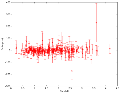
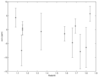
Astrophysical data: we will use both the spectroscopic measurements of of Webb et al. Webb et al. (2011) (a large dataset of 293 archival data measurements) and the smaller but more recent dataset of 11 dedicated measurements listed in Table 1. The latter include the early results of the UVES Large Program for Testing Fundamental Physics Molaro et al. (2013); Evans et al. (2014), which is expected to be the one with a better control of possible systematics. Figure 1 depicts both of these datasets.
| Object | z | (ppm) | Spectrograph | Ref. |
|---|---|---|---|---|
| 3 sources | 1.08 | HIRES | Songaila and Cowie (2014) | |
| HS15491919 | 1.14 | UVES/HIRES/HDS | Evans et al. (2014) | |
| HE05154414 | 1.15 | UVES | Molaro et al. (2008) | |
| HE05154414 | 1.15 | HARPS/UVES | Chand et al. (2006) | |
| HS15491919 | 1.34 | UVES/HIRES/HDS | Evans et al. (2014) | |
| HE00012340 | 1.58 | UVES | Agafonova et al. (2011) | |
| HE11041805A | 1.66 | HIRES | Songaila and Cowie (2014) | |
| HE22172818 | 1.69 | UVES | Molaro et al. (2013) | |
| HS19467658 | 1.74 | HIRES | Songaila and Cowie (2014) | |
| HS15491919 | 1.80 | UVES/HIRES/HDS | Evans et al. (2014) | |
| Q1101264 | 1.84 | UVES | Molaro et al. (2008) |
We use these datasets to constrain the dynamical dark energy models which will be described in the following sections. The behavior of is determined by Eq.(6) for canonical equations of state () and Eq.(7) for phantom equations of state (). While in Martins and Pinho (2015); Martins et al. (2015) we studied models whose equations of state were parametrized by a single parameter (its present day value, ) here we relax this assumption and study more general models.
For comparison, we also list here the available direct constraints on the dimensionless Eötvös parameter, quantifying violations to the Weak Equivalence Principle. These stem from torsion balance tests, leading to Wagner et al. (2012)
| (14) |
while from lunar laser ranging one obtains Müller et al. (2012)
| (15) |
Both of these are quoted with their one-sigma uncertainties.
Our main interest is in obtaining constraints on and the dark energy parameters. For this reason we will fix the Hubble parameter to be km/s/Mpc and the matter density to be , and further assume a flat universe, so . This choice of cosmological parameters is fully consistent with the supernova and Hubble parameter data we use.
Moreover, in Martins and Pinho (2015); Martins et al. (2015) we have explicitly verified that allowing , or the curvature parameter to vary (within observationally reasonable ranges) and marginalizing over them does not significantly change our results. This should be intuitively clear: a parts-per-million variation of cannot noticeably affect these cosmological parameters. It is clear that the critical cosmological parameters here are the ones describing the dark energy equation of state, as in Class I models they will be correlated with —cf. Eqs.(6–7). We therefore consider 3D grids of , and the additional (model-dependent) parameter, and use standard maximum likelihood techniques to compare the models and the data. Flat priors on the relevant parameters will be used, unless otherwise stated.
IV Standard dark energy
We will start by studying canonical dark energy models in which the fraction of the dark energy density tends to zero at high redshift. Note that in this case the relative variation of will tend to a constant in the same limit. We will study the standard CPL parametrization but will also aim to gain some insight on the degree of model-dependence of these results by considering an alternative parametrization.
IV.1 CPL parametrization
In the Chevallier-Polarski-Linder Chevallier and Polarski (2001); Linder (2003) parametrization the dark energy equation of state is written as
| (16) |
where is its present value and is the coefficient of the time-dependent term. The redshift dependence of this parametrization is not intended to mimic a particular model for dark energy, but rather to allow to probe possible deviations from the CDM standard paradigm without the assumption of any underlying theory. Nevertheless, we can assume that also this kind of dark energy is produced by a scalar field, coupled to the electromagnetic sector. In this model the fraction of energy density provided by the scalar field is easily found to be
| (17) |
where is the present time matter density and we have also assumed a flat universe. Figure 2 illustrates the behavior of and in this model for realistic parameter choices, compatible with our cosmological datasets and the recent Planck collaboration results Ade et al. (2015) (which are also used to choose priors for and ).
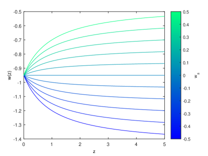
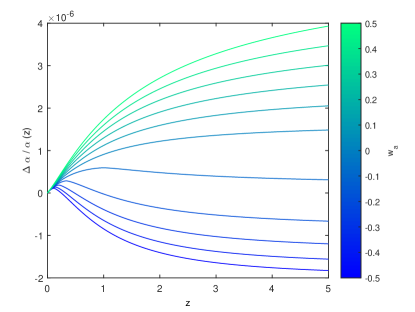
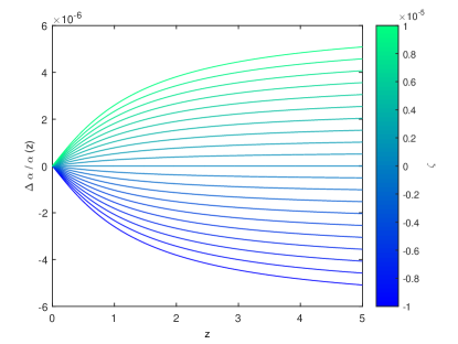
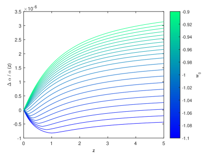
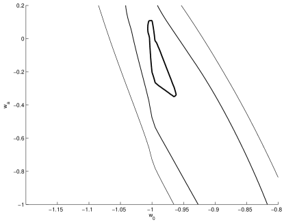
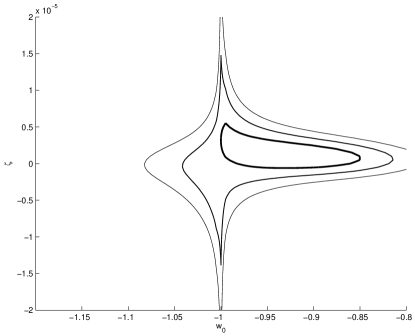
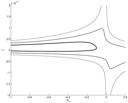
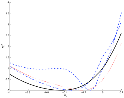
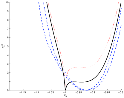
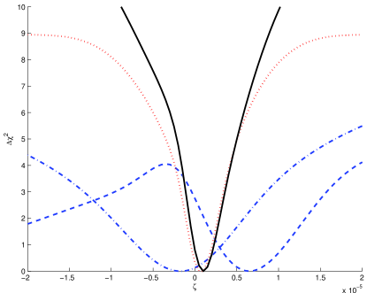
Figure 3 shows the 2D marginalized constraints from our full (i.e., cosmological plus atomic clock plus astrophysical) datasets in the three relevant planes, with the remaining parameter marginalized. One, two and three sigma contours are shown in all cases. Several degeneracies are clearly visible which among other things imply that no significant constraints can be obtained on . However, this is not the case for the other two parameters. As explained in previous work Martins and Pinho (2015); Martins et al. (2015), the cosmological datasets effectively provide us with priors on the dark energy behavior close to the present day, partially breaking otherwise unavoidable degeneracies with and thereby enabling substantive constraints on it.
Figure 4 shows the 1D marginalized likelihoods for each of the three parameters, for the full dataset we use as well as for several choices of sub-sets. Specifically one may note the qualitatively different behavior of the Webb et al. and dedicated measurements: the former is not consistent with the null result for Webb et al. (2011), and we correspondingly find a one sigma preference for a non-zero coupling . However, this data is compatible with the null result at the two sigma level. On the other hand, the Table 1 data is fully compatible with the null result. Finally, the local atomic clock measurement Rosenband et al. (2008) is more constraining than the astrophysical measurements.
From these we obtain a very weak 1D marginalized constraint on
| (18) |
while that for is stronger
| (19) |
and that for the coupling even more so
| (20) |
| (21) |
Finally for the Eötvös parameter we obtain
| (22) |
Compared to earlier results Martins and Pinho (2015); Martins et al. (2015) the constraint on becomes weaker (due to the additional freedom provided by the largely unconstrained ) while that on (and consequently that on ) become correspondingly stronger. This is to be expected since is correlated with the dark energy equation of state parameters: with the equation of state allowed to be further away from a cosmological constant, larger variations of also become possible, and the existing measurements therefore impose a tighter constraint on . This effect was also noticed in the case of the forecasts discussed in Calabrese et al. (2014).
IV.2 Mukhanov parametrization
It is interesting to assess the model-dependence of the above constraints on and , and a simple way to do so is to repeat the analysis for a different parametrization of the dark energy equation of state. We will do this through a parametrization recently discussed by Mukhanov in Mukhanov (2013). This was introduced in an inflationary context, but it can be trivially applied for the case of the recent acceleration of the universe.
In this parametrization (which we will refer to as MKH) the dark energy equation of state is
| (23) |
where is its present day value and the slope controls the overall redshift dependence. Specifically corresponds to freezing models, to a constant equation of state and to thawing models, in the classification of Caldwell and Linder (2005). This corresponds to the following behavior of the dark energy density
| (24) | |||||
| (25) |
and it is easy to verify that this has the correct behavior in the appropriate limits.
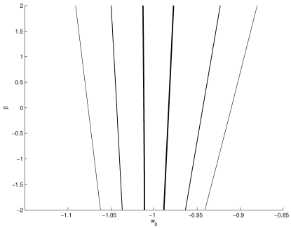
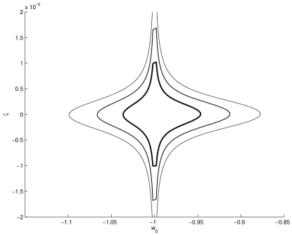
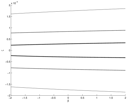
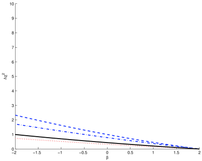
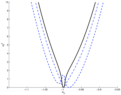
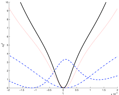
The analysis can now be repeated for this model, and the results are summarized in Figs. 5 and 6, which can be compared to Figs. 3 and 4. Again there is no significant constraint on the slope , although freezing models (with ) are comparatively more constrained than thawing ones (with ). Physically the reason for this is clear: for a given value of , a freezing model leads to a larger variation of than an thawing one, and is therefore more tightly constrained by the datasets we are considering.
In this case the 1D marginalized constraint on is
| (26) |
| (27) |
while for the coupling we now find
| (28) |
leading to
| (29) |
V Early dark energy
We now study the Early Dark Energy (EDE) class of models Doran and Robbers (2006). In this case the dark energy density fraction is
| (30) |
while the dark energy equation of state is
| (31) |
here is the scale factor. The energy density has a scaling behavior evolving with time and approaching a finite constant in the past, rather than approaching zero as was the case for the models in the previous section. A flat universe is also assumed.
The present day value of the equation of state is , and the equation of state follows the behavior of the dominant component at each cosmic time, with during radiation domination, and during matter domination. Even though this is a phenomenological parametrization, we will again assume that this kind of dark energy is the result of an underlying scalar field, which couples to the electromagnetic sector. Figure 7 illustrates the behavior of and in this model for realistic parameter choices, compatible with the recent Planck collaboration results Ade et al. (2015); in particular we use .
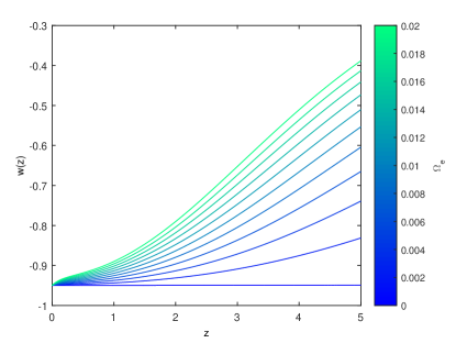
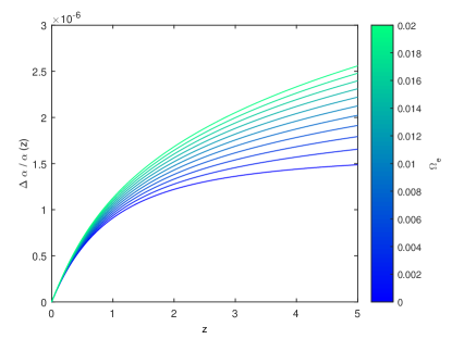
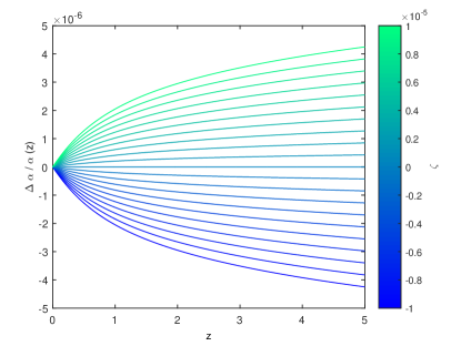
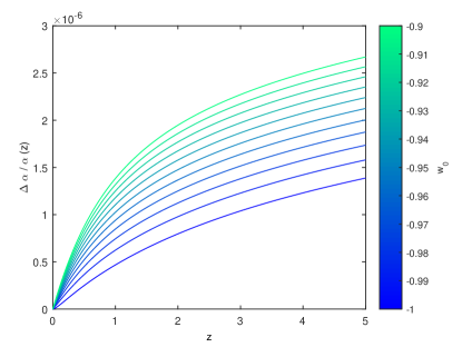
V.1 Flat prior
We start by studying the EDE model using a flat prior on and further assuming that . We then carry out an analysis similar to that of the previous section, the results of which can be seen in Figs. 8 and 9.
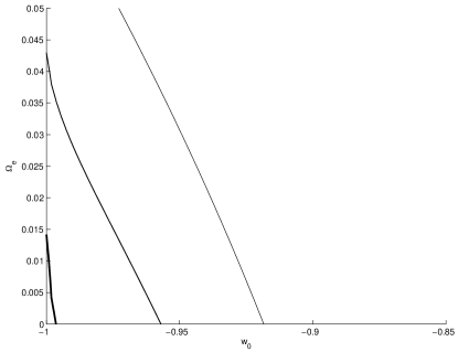
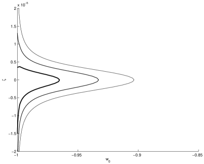
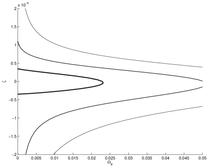
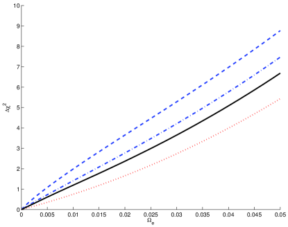
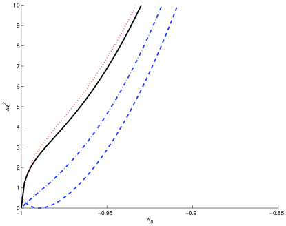
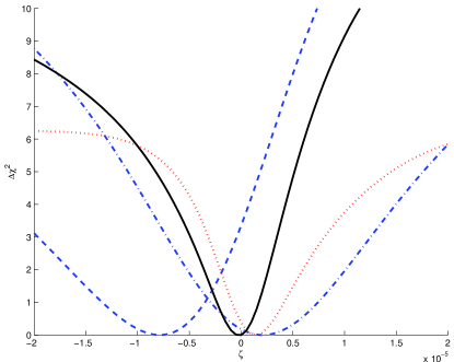
In this case the correlation between and is also clear, although it is partially broken by the cosmological data. The same happens with the early dark energy density, for which we can also obtain non-trivial constraints. Here we obtain the following 1D marginalized constraints
| (32) |
which is about a factor of 3 weaker than the standard one without allowing for possible variations. On the other hand, for we obtain
| (33) |
| (34) |
and finally for the coupling we obtain
| (35) |
leading to
| (36) |
Here, by comparison to the CPL case, the slightly stronger constraints on the dark energy sector imply slightly weaker constraints on the coupling .
V.2 Logarithmic prior
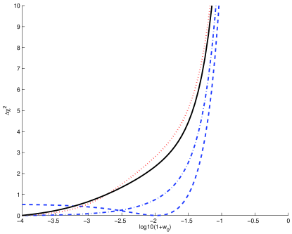
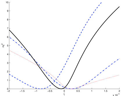
We finally study the impact of our choices of priors, specifically by assessing the impact of using a logarithmic (rather than flat) prior on . The results can now be seen in Figs. 10 and 11.
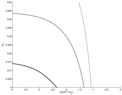
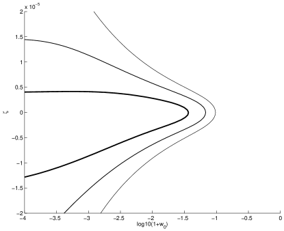
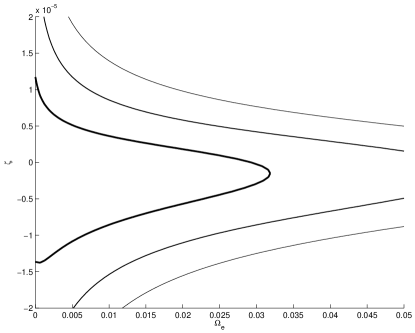
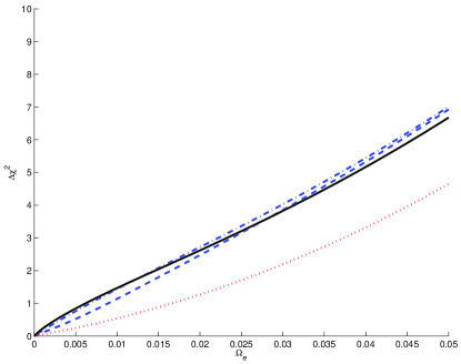
The 1D marginalized constraints now become
| (37) |
which is about ten percent stronger than the flat prior case. For the constraints are unchanged,
| (38) |
| (39) |
and finally the constraint on the coupling becomes weaker as well as asymmetric
| (40) |
leading to
| (41) |
note that even in this case this constraint is still marginally stronger than the current direct bounds.
VI Conclusions and outlook
We have used a combination of astrophysical spectroscopy and local laboratory tests of the stability of the fine-structure constant , complemented by background cosmological datesets, to constrain several broad class of dynamical dark energy models where the same degree of freedom is responsible for both the dark energy and a variation of . In these models, which are more general than the ones previously studied Martins and Pinho (2015); Martins et al. (2015), the redshift dependence of is a function both of a fundamental physics parameter (the dimensionless coupling of the scalar field to the electromagnetic sector) and background ’dark cosmology’ parameters, including the present day dark energy equation of state .
Our analysis confirms that, despite some mild dependence on the underlying model and the choice of priors, the combination of cosmological, astrophysical and atomic clock data leads to tight and competitive constraints on the dimensionless coupling of the scalar field to the electromagnetic sector as well as on . Current data is consistent with the standard CDM paradigm where and .
Presently these constraints are dominated by the atomic clock tests Rosenband et al. (2008), which are only sensitive to the dark energy equation of state today. This is one of the reasons why additional parameters such as in the CPL parametrization and in the MKH parametrization are weakly constrained by the present data. Improvements in astrophysical measurements will allow significantly stronger constraints on a larger parameter space. Forthcoming high-resolution ultra-stable spectrographs such as ESPRESSO and ELT-HIRES will be ideal for this task. A roadmap for these studies is outlined in Martins (2014), and more detailed forecasts of the future impact of these measurements may be found in Leite et al. (2014); Leite and Martins (2015).
Importantly, in the classes of models we have studied the dynamical degree of freedom responsible for the dark energy and the variation inevitably couples to nucleons (through the dependence of their masses) and leads to violations of the Weak Equivalence Principle. Our bounds on the coupling can therefore be used to obtain indirect bounds on the Eötvös parameter . Despite the aforementioned model dependence, these bounds are stronger than the current direct ones, typically by as much as one order of magnitude. Broadly speaking they are at the few level.
We note that the forthcoming MICROSCOPE mission, currently scheduled for launch in April 2016, should reach sensitivity Bergé et al. (2015). Should this measure a value of larger than that in our bounds, this would rule out the Class I models we have studied here, and specifically the physically crucial assumption of the coupling of the dynamical dark energy field to the electromagnetic sector. Alternatively, a MICROSCOPE detection of a large would imply that the measurements of on which they rely are incorrect and dominated by unaccounted systematics.
For the same reason, the next generation of high-resolution ultra-stable spectrographs will also provide significantly tighter constraints on . Specifically, for Class I models and on the basis of the forecasts of Leite et al. (2014); Leite and Martins (2015), we may conservatively expect a sensitivity of few for ESPRESSO and for ELT-HIRES. The latter is comparable to the expected sensitivity of the proposed STEP satellite Overduin et al. (2012).
Thus the next decade will bring forth tests of these cornerstone principles with unprecedented accuracy. Null results from STEP and the E-ELT would then imply that any putative coupling of light scalar fields to the standard model would need to be unnaturally small, which in turn would mean that either WEP violating fields do not exist at all in nature or that these couplings are suppressed by some currently unknown mechanism. This would be an astrophysical analog of the strong CP problem in Quantum Chromodynamics Peccei and Quinn (1977). In any case, our analysis shows that astrophysical tests of the stability of fundamental couplings are a crucial probe of fundamental physics and cosmology.
Acknowledgements.
We are grateful to Ana Catarina Leite and David Corre for many helpful discussions on the subject of this work. This work was done in the context of project PTDC/FIS/111725/2009 (FCT, Portugal). CJM is also supported by an FCT Research Professorship, contract reference IF/00064/2012, funded by FCT/MCTES (Portugal) and POPH/FSE (EC). A.G. and J.L. acknowledge financial support from Programa Joves i Ciència, funded by Fundació Catalunya-La Pedrera.References
- Riess et al. (1998) A. G. Riess et al. (Supernova Search Team), Astron.J. 116, 1009 (1998), arXiv:astro-ph/9805201 [astro-ph] .
- Perlmutter et al. (1999) S. Perlmutter et al. (Supernova Cosmology Project), Astrophys.J. 517, 565 (1999), arXiv:astro-ph/9812133 [astro-ph] .
- Aad et al. (2012) G. Aad et al. (ATLAS Collaboration), Phys.Lett. B716, 1 (2012), arXiv:1207.7214 [hep-ex] .
- Chatrchyan et al. (2012) S. Chatrchyan et al. (CMS Collaboration), Phys.Lett. B716, 30 (2012), arXiv:1207.7235 [hep-ex] .
- Carroll (1998) S. M. Carroll, Phys.Rev.Lett. 81, 3067 (1998), arXiv:astro-ph/9806099 [astro-ph] .
- Uzan (2011) J.-P. Uzan, Living Rev.Rel. 14, 2 (2011), arXiv:1009.5514 [astro-ph.CO] .
- Martins (2014) C. J. A. P. Martins, Gen.Rel.Grav. 47, 1843 (2014), arXiv:1412.0108 [astro-ph.CO] .
- Webb et al. (2011) J. Webb, J. King, M. Murphy, V. Flambaum, R. Carswell, et al., Phys.Rev.Lett. 107, 191101 (2011), arXiv:1008.3907 [astro-ph.CO] .
- Molaro et al. (2013) P. Molaro, M. Centurion, J. Whitmore, T. Evans, M. Murphy, et al., Astron.Astrophys. 555, A68 (2013), arXiv:1305.1884 [astro-ph.CO] .
- Evans et al. (2014) T. M. Evans, M. T. Murphy, J. B. Whitmore, T. Misawa, M. Centurion, S. D’Odorico, S. Lopez, C. J. A. P. Martins, P. Molaro, P. Petitjean, H. Rahmani, R. Srianand, and M. Wendt, M.N.R.A.S. 445, 128 (2014).
- Amendola et al. (2012) L. Amendola, A. C. O. Leite, C. J. A. P. Martins, N. Nunes, P. O. J. Pedrosa, et al., Phys.Rev. D86, 063515 (2012), arXiv:1109.6793 [astro-ph.CO] .
- Leite et al. (2014) A. C. O. Leite, C. J. A. P. Martins, P. O. J. Pedrosa, and N. Nunes, Phys.Rev. D90, 063519 (2014), arXiv:1409.3963 [astro-ph.CO] .
- Leite and Martins (2015) A. Leite and C. Martins, Phys. Rev. D91, 103519 (2015), arXiv:1505.05529 [astro-ph.CO] .
- Martins and Pinho (2015) C. J. A. P. Martins and A. M. M. Pinho, Phys. Rev. D91, 103501 (2015), arXiv:1505.02196 [astro-ph.CO] .
- Martins et al. (2015) C. J. A. P. Martins, A. M. M. Pinho, R. F. C. Alves, M. Pino, C. I. S. A. Rocha, and M. von Wietersheim, JCAP 1508, 047 (2015), arXiv:1508.06157 [astro-ph.CO] .
- Dvali and Zaldarriaga (2002) G. Dvali and M. Zaldarriaga, Phys.Rev.Lett. 88, 091303 (2002), arXiv:hep-ph/0108217 [hep-ph] .
- Chiba and Kohri (2002) T. Chiba and K. Kohri, Prog. Theor. Phys. 107, 631 (2002), arXiv:hep-ph/0111086 [hep-ph] .
- Caldwell and Linder (2005) R. R. Caldwell and E. V. Linder, Phys. Rev. Lett. 95, 141301 (2005), arXiv:astro-ph/0505494 [astro-ph] .
- Chevallier and Polarski (2001) M. Chevallier and D. Polarski, Int. J. Mod. Phys. D10, 213 (2001), arXiv:gr-qc/0009008 [gr-qc] .
- Linder (2003) E. V. Linder, Phys. Rev. Lett. 90, 091301 (2003), arXiv:astro-ph/0208512 [astro-ph] .
- Doran and Robbers (2006) M. Doran and G. Robbers, JCAP 0606, 026 (2006), arXiv:astro-ph/0601544 [astro-ph] .
- Mukhanov (2013) V. Mukhanov, Eur. Phys. J. C73, 2486 (2013), arXiv:1303.3925 [astro-ph.CO] .
- Calabrese et al. (2011) E. Calabrese, E. Menegoni, C. J. A. P. Martins, A. Melchiorri, and G. Rocha, Phys.Rev. D84, 023518 (2011), arXiv:1104.0760 [astro-ph.CO] .
- Nunes and Lidsey (2004) N. J. Nunes and J. E. Lidsey, Phys. Rev. D69, 123511 (2004), arXiv:astro-ph/0310882 [astro-ph] .
- Vielzeuf and Martins (2014) P. E. Vielzeuf and C. J. A. P. Martins, Mem.Soc.Ast.It. 85, 155 (2014), arXiv:1309.7771 [astro-ph.CO] .
- Damour and Donoghue (2010) T. Damour and J. F. Donoghue, Class. Quant. Grav. 27, 202001 (2010), arXiv:1007.2790 [gr-qc] .
- Suzuki et al. (2012) N. Suzuki, D. Rubin, C. Lidman, G. Aldering, R. Amanullah, et al., Astrophys.J. 746, 85 (2012), arXiv:1105.3470 [astro-ph.CO] .
- Farooq and Ratra (2013) O. Farooq and B. Ratra, Astrophys.J. 766, L7 (2013), arXiv:1301.5243 [astro-ph.CO] .
- Calabrese et al. (2014) E. Calabrese, M. Martinelli, S. Pandolfi, V. F. Cardone, C. J. A. P. Martins, S. Spiro, and P. E. Vielzeuf, Phys.Rev. , 083509 (2014), arXiv:1311.5841 [astro-ph.CO] .
- Rosenband et al. (2008) T. Rosenband, D. Hume, P. Schmidt, C. Chou, A. Brusch, L. Lorini, W. Oskay, R. Drullinger, T. Fortier, J. Stalnaker, S. Diddams, W. Swann, N. Newbury, W. Itano, D. Wineland, and J. Bergquist, Science 319, 1808 (2008).
- Luo et al. (2011) F. Luo, K. A. Olive, and J.-P. Uzan, Phys. Rev. D84, 096004 (2011), arXiv:1107.4154 [hep-ph] .
- Ferreira et al. (2014) M. C. Ferreira, O. Frigola, C. J. A. P. Martins, A. M. R. V. L. Monteiro, and J. Solà, Phys. Rev. D89, 083011 (2014), arXiv:1405.0299 [astro-ph.CO] .
- Ferreira and Martins (2015) M. Ferreira and C. Martins, Phys. Rev. D91, 124032 (2015), arXiv:1506.03550 [astro-ph.CO] .
- Songaila and Cowie (2014) A. Songaila and L. Cowie, Astrophys.J. 793, 103 (2014), arXiv:1406.3628 [astro-ph.CO] .
- Molaro et al. (2008) P. Molaro, D. Reimers, I. I. Agafonova, and S. A. Levshakov, Eur.Phys.J.ST 163, 173 (2008), arXiv:0712.4380 [astro-ph] .
- Chand et al. (2006) H. Chand, R. Srianand, P. Petitjean, B. Aracil, R. Quast, and D. Reimers, Astron.Astrophys. 451, 45 (2006), astro-ph/0601194 .
- Agafonova et al. (2011) I. I. Agafonova, P. Molaro, S. A. Levshakov, and J. L. Hou, Astron.Astrophys. 529, A28 (2011), arXiv:1102.2967 [astro-ph.CO] .
- Wagner et al. (2012) T. A. Wagner, S. Schlamminger, J. H. Gundlach, and E. G. Adelberger, Class. Quant. Grav. 29, 184002 (2012), arXiv:1207.2442 [gr-qc] .
- Müller et al. (2012) J. Müller, F. Hofmann, and L. Biskupek, Class. Quant. Grav. 29, 184006 (2012).
- Ade et al. (2015) P. A. R. Ade et al. (Planck), (2015), arXiv:1502.01589 [astro-ph.CO] .
- Bergé et al. (2015) J. Bergé, P. Touboul, and M. Rodrigues (MICROSCOPE), Proceedings, 10th International LISA Symposium, J. Phys. Conf. Ser. 610, 012009 (2015), arXiv:1501.01644 [gr-qc] .
- Overduin et al. (2012) J. Overduin, F. Everitt, P. Worden, and J. Mester, Class. Quant. Grav. 29, 184012 (2012), arXiv:1401.4784 [gr-qc] .
- Peccei and Quinn (1977) R. D. Peccei and H. R. Quinn, Phys. Rev. Lett. 38, 1440 (1977).