Spin evolution of a proto-neutron star

Abstract

We study the evolution of the rotation rate of a proto-neutron star, born in a core-collapse supernova, in the first seconds of its life. During this phase, the star evolution can be described as a sequence of stationary configurations, which we determine by solving the neutrino transport and the stellar structure equations in general relativity. We include in our model the angular momentum loss due to neutrino emission. We find that the requirement of a rotation rate not exceeding the mass-shedding limit at the beginning of the evolution implies a strict bound on the rotation rate at later times. Moreover, assuming that the proto-neutron star is born with a finite ellipticity, we determine the emitted gravitational wave signal, and estimate its detectability by present and future ground-based interferometric detectors.

I Introduction

When a supernova explodes, it leaves a hot, lepton-rich and (presumably) rapidly rotating remnant: a proto-neutron star (PNS). In the early stages of its evolution, the PNS cools down and loses its high lepton content, while its radius and rotation rate decrease. In this phase, a huge amount of energy and of angular momentum is released, mainly due to neutrino emission Burrows and Lattimer (1986); Keil and Janka (1995); Pons et al. (1999). A fraction of this energy is expected to be emitted in the gravitational wave channel; indeed, as a consequence of the violent collapse non-radial oscillations can be excited, making PNSs promising sources for present and future gravitational detectors Ferrari et al. (2003); Ott (2009); Burgio et al. (2011); Fuller et al. (2015).

In the first tenths of seconds after its birth, the PNS is turbulent and characterized by large instabilities. During the next tens of seconds, it undergoes a more quiet, “quasi-stationary” evolution (the Kelvin-Helmholtz phase), which can be described as a sequence of equilibrium configurations Burrows and Lattimer (1986); Pons et al. (1999). In this article, we study the evolution of the rotation rate of a PNS during this quasi-stationary, Kelvin-Helmholtz phase. An accurate modeling of this phase is needed, for instance, to compute the frequencies of the PNS gravitational wave emission. Moreover, it provides a link bewteen supernova explosions, a phenomenon which is still not fully understood, and the properties of the observed population of young pulsars. Current models of the evolution of progenitor stars Heger et al. (2005), combined with numerical simulations of core collapse and explosion (see e.g. Thompson et al. (2005); Ott et al. (2006); Hanke et al. (2013); Couch and Ott (2015); Nakamura et al. (2014)), do not allow sufficiently accurate estimates of the expected rotation rate of newly born PNSs; they only show that the minimum rotation period at the onset of the Kelvin-Helmoltz phase can be as small as few ms, if the spin rate of the progenitor is sufficiently high. On the other hand, astrophysical observations of young pulsar populations (see Miller and Miller (2014) and references therein) show typical periods $\gtrsim~{}100$ ms.

The quasi-stationary evolution of a PNS driven by neutrino transport in a spherically symmetric space-time has been extensively studied in the past, quite often adopting an equation of state (EoS) obtained within a finite-temperature, field-theoretical model solved at the mean field level Pons et al. (1999, 2001a, 2001b); Roberts (2012). This approach yields a sequence of thermodynamical profiles describing the structure and the early evolution of a non-rotating PNS. A different approach has been used in Burgio et al. (2011), where an EoS obtained within a finite-temperature many-body theory approach was employed, but the neutrino transport equations were not explicitly solved (a set of entropy and lepton fraction profiles were adopted, having the same qualitative behaviour as those of Pons et al. (1999)). We also mention that the non-radial oscillations of the quasi-stationary configurations obtained with these different approaches have been studied in Ferrari et al. (2003, 2004); Burgio et al. (2011), where the quasi-normal mode frequencies of the gravitational waves emitted in the early PNS life were computed.

The evolution of rotating PNSs has been studied in Villain et al. (2004), where the thermodynamical profiles obtained in Pons et al. (1999) for a non-rotating PNS were employed as effective one-parameter EoSs; the rotating configurations were obtained using the non-linear BGSM code Gourgoulhon et al. (1999) to solve Einstein’s equations. A similar approach has been followed in Martinon et al. (2014), which used the profiles of Pons et al. (1999) and Burgio et al. (2011). The main limitations of these works are the following.

• The evolution of the PNS rotation rate is due not only to the change in the moment of inertia (i.e., to the contraction), but also to the angular momentum change due to neutrino emission Epstein (1978). This was neglected in Villain et al. (2004), and described with an heuristic formula in Martinon et al. (2014).

• As we shall discuss in this paper, when the PNS profiles describing a non-rotating star are treated as an effective EoS, one can obtain configurations which are unstable to radial perturbations.

In this article, we study the quasi-stationary evolution of a spherically symmetric PNS, solving the relativistic equations of neutrino transport and of stellar structure. The details of our code will be discussed in Camelio et al. (2016), where it will be applied to more recent EoSs. Here, we employ the same EoS used in Pons et al. (1999) (i.e. GM3 Glendenning and Moszkowski (1991)), to study the spin evolution of the PNS in its first tens of seconds of life. To model an evolving, rotating PNS, we use the profiles of entropy per baryon and lepton fraction $s(a)$, $Y_{L}(a)$ ($a$ is the number of baryons enclosed in a sphere passing through the point considered) obtained with our evolution code which describes a non-rotating PNS. Our approach is different from that used in Villain et al. (2004), as will be discussed in detail in Sec III.2. In order to determine the PNS spin evolution, we model the evolution of angular momentum (due to neutrino emission) using Epstein’s formula Epstein (1978). We also discuss the gravitational wave emission which could be associated with this process.

The plan of the paper is as follows. In Sec. II we briefly describe our approach to model the PNS evolution in its quasi-stationary phase. In Sec. III we describe our model of a rotating PNS. In Sec. IV we show our results, and in Sec. V we draw our conclusions. The details of the slowly rotating model are described in Appendix A.

II Early evolution of a proto-neutron star

The quasi-stationary, Kelvin-Helmholtz phase of a PNS starts few hundreds of ms after the core bounceBurrows and Lattimer (1986); Pons et al. (1999). This phase consists of two evolutionary stages. In the first few tens of seconds, neutrinos diffuse from the low-entropy core to the high-entropy envelope, deleptonizing the core and increasing its temperature. In the second phase, the star is lepton poor but hot, the entropy gradient is smoothed out, and thermally produced neutrinos cool down the PNS. After about one minute, the star becomes transparent to neutrinos and can be considered as a “mature” neutron star, with a radius of $\sim 10-15$ km and a temperature $<1$ MeV.

The PNS evolution in the Kelvin-Helmholtz phase can be considered as a sequence of quasi-stationary configurations, because the hydrodynamical timescale is much smaller than the evolution timescale. Following Pons et al. (1999), we model this phase by solving the general relativistic neutrino transport equations coupled with the structure equations, assuming spherical symmetry. In each quasi-stationary configuration, the spacetime metric has the form

$$ds^{2}=-e^{\phi(r)}dt^{2}+e^{\lambda(r)}dr^{2}+r^{2}(d\theta^{2}+\sin^{2}\theta d\varphi^{2})\,,$$ (1)

where $\phi(r)$ and $\lambda(r)$ are radial functions, obtained by solving the Tolman-Oppenheimer-Volkov (TOV) equations (in this paper we use geometrized units, in which $c=G=1$). The perfect fluid of the star is described by the stress-energy tensor $T_{\mu\nu}=(\epsilon+p)u_{\mu}u_{\nu}+pg_{\mu\nu}$, where $u^{\mu}=(e^{-\phi/2},0,0,0)$ is the fluid four-velocity and $\epsilon,p$ are the energy density and pressure of the fluid, respectively. The gravitational mass inside a radius $r$ is $m(r)=r(1-e^{-\lambda})/2$. At the surface of the star, $r=R$, the pressure vanishes and the metric matches with the exterior Schwarzschild metric, with $M=m(R)$ as the gravitational mass of the star. We also define the baryon number inside a radius $r$,

$$a(r)=4\pi\int_{0}^{r}e^{\lambda/2}n_{b}r^{\prime 2}dr^{\prime}\,,$$ (2)

where $n_{b}$ is the baryon number density. The position inside the star can be described either by the coordinate $r$, or by the enclosed baryon number $a$. We also define the rest-mass density $\rho=m_{n}n_{b}$ ($m_{n}$ is the neutron mass), and the baryon mass of the star $M_{b}=m_{n}a(R)$. We will use $M_{b}=1.60~{}M_{\odot}$, which corresponds, in the calculations of this paper, to a gravitational mass of $1.55~{}M_{\odot}$ at $200$ ms from the core bounce, which reduces to $\sim 1.4~{}M_{\odot}$ in the first ten seconds of life of the PNS.

Since the PNS has a temperature of several MeV, its EoS is non-barotropic, and can be written as

$$\epsilon=\epsilon(p,s,\{Y_{i}\}_{i})\,,$$ (3)

where $s$ is the entropy per baryon, and $Y_{i}=n_{i}/n_{b}$ is the fraction of the $i$-th specie, with number density $n_{i}$. Assuming that the matter is in beta equilibrium, the dependence on the composition $\{Y_{i}\}_{i}$ can be cast into a dependence on only the electron-type lepton fraction $Y_{L}=n_{L}/n_{b}$. Different choices of thermodynamical variables are possible, for instance replacing the entropy per baryon $s$ with the temperature $T$. In this paper, we use the finite-temperature EoS GM3 of Glendenning and Moszkowski Glendenning and Moszkowski (1991), obtained within a field-theoretical model solved at the mean field level, where the interactions between baryons are mediated by the exchange of mesons; it contains only nucleonic degrees of freedom. This is the same EoS employed in Pons et al. (1999); we consider the case of matter composed by electrons, protons and neutrons. More recent EoSs, based on a many-body theory approach, will be considered in a future work Camelio et al. (2016).

In order to solve the TOV equations, we need to know, at each point, the energy density as a function of the pressure; thus, we need to know the EoS and the thermodynamical profiles $s(a)$, $Y_{L}(a)$, which are obtained by solving the transport equations

$$\frac{\partial Y_{L}}{\partial t}+\frac{\partial(4\pi e^{\phi/2}r^{2}F_{\nu})}{\partial a} =0\,,$$ (4)

$$T\frac{\partial s}{\partial t}+\mu_{\nu}\frac{\partial Y_{L}}{\partial t}+e^{-\phi/2}\frac{\partial(4\pi e^{\phi}r^{2}H_{\nu})}{\partial a} =0\,,$$ (5)

where $F_{\nu}$ and $H_{\nu}$ are, respectively, the neutrino number and energy fluxes

$$F_{\nu}={} -\frac{\mathrm{e}^{-\frac{\lambda+\phi}{2}}T^{2}}{6\pi^{2}\hbar^{3}}\Bigg{[}D_{3}\frac{\partial(T\mathrm{e}^{\phi/2})}{\partial r}+(T\mathrm{e}^{\phi/2})D_{2}\frac{\partial\eta}{\partial r}\Bigg{]}\,,$$ (6)

$$H_{\nu}={} -\frac{\mathrm{e}^{-\frac{\lambda+\phi}{2}}T^{3}}{6\pi^{2}\hbar^{3}}\Bigg{[}D_{4}\frac{\partial(T\mathrm{e}^{\phi/2})}{\partial r}+(T\mathrm{e}^{\phi/2})D_{3}\frac{\partial\eta}{\partial r}\Bigg{]}\,,$$ (7)

where $\eta=\mu_{\nu}/T$ is the electron-type neutrino degeneracy parameter and $D_{n}$ are the neutrino diffusion coefficients, which are computed assuming the diffusion approximation Pons et al. (1999). In order to preserve causality and stabilize the code in the semi-transparent regions near the PNS surface, we apply a flux-limiter Levermore and Pomraning (1981).

Our code evolves the PNS by iteratively solving, at each time-step, (i) the transport equations (4) and (5) using an implicit scheme and (ii) the TOV equations by relaxation method. The time evolution keeps the baryon mass $M_{b}$ constant, and provides, at each time-step, a quasi-stationary configuration of the (non-rotating) star, described by the profiles of all the thermodynamical quantities ($p$, $\epsilon$, $n_{b}$, $s$, $Y_{L}$, etc.) as functions of $a$ (or of $r$). We start our integration at $200$ ms from core bounce. The initial profiles (which are the same employed in Pons et al. (1999)) are the result of core-collapse simulations Wilson and Mayle (1989). In Figures 1 and 2 we show the evolutionary profiles of the entropy per baryon $s$ and the electron-type lepton fraction $Y_{L}$ as functions of the enclosed baryon mass. We have checked that the total energy and lepton number are conserved during the evolution within a few percent in the early stages of the evolution, and with more accuracy in later stages. We remark that this error can be significantly reduced by reducing the timestep; however, this accuracy is sufficient for the aims of this work. Our code will be described in detail in a future work Camelio et al. (2016).

Recently, different approaches have been applied in the study of the PNS evolution (see e.g. Roberts (2012)), in which the neutrino spectrum is described with greater accuracy by means of multi-group codes. However, since in this work we are not interested in the details of the neutrino emission, we prefer to employ a simpler and faster energy-averaged approach (as in Pons et al. (1999)). As mentioned above, our code also employs a flux-limiter Levermore and Pomraning (1981), which makes it difficult to establish the precise location of the neutrinosphere. Both the neutrinosphere and the neutrino spectra are better determined with more complex core-collapse codes, which however are far slower, while our PNS code is suitable to run for longer evolution times. Typical core-collapse codes run for at most $500$ ms after core bounce, whereas we can easily explore the first minute of PNS life, at the end of which the star becomes neutrino-transparent.

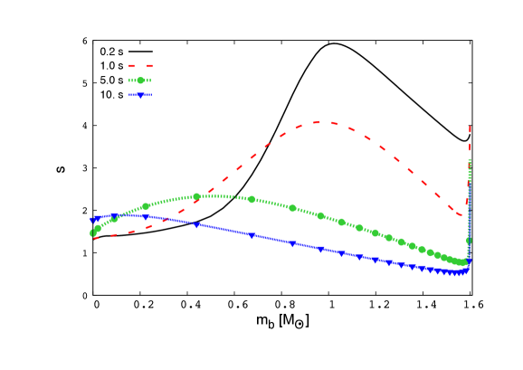
Figure 1: Entropy per baryon as a function of the enclosed baryon mass $m_{b}=m_{n}a$ at $t=0.2,1,5,10$ s ($k_{\mathrm{B}}=1$).

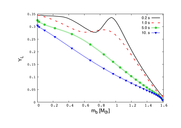
Figure 2: Electron-type lepton fraction as a function of the enclosed baryon mass at $t=0.2,1,5,10$ s.

III A model of rotating proto-neutron stars

III.1 Slowly rotating stars in general relativity

We model a rotating PNS using the perturbative approach of Hartle and Thorne Hartle (1967); Hartle and Thorne (1968) (see also Benhar et al. (2005)). The rotating star is described as a stationary perturbation of a spherically symmetric background, for small values of the angular velocity $\Omega=2\pi\nu$, i.e., $\nu\ll\nu_{ms}$ ($\nu_{ms}$ is the mass-shedding frequency, at which the star starts losing mass at the equator, see Sec. III.4). As shown in Martinon et al. (2014), this “slow rotation” approximation is reasonably accurate for rotation rates up to $\sim 0.8$ of the mass-shedding limit, providing values of mass, equatorial radius and moment of inertia which differ by $\lesssim 0.5\%$ from those obtained with fully relativistic, nonlinear simulations. In our approach we assume uniform rotation; PNSs are expected to have a significant amount of differential rotation at birth Janka and Mönchmeyer (1989) which, however, is likely to be removed by viscous mechanisms, such as, for instance, magnetorotational instability Mösta et al. (2015), in a fraction of a second.

This work should be considered as a first step towards a more detailed description of rotating PNSs, in which we shall include differential rotation.

The spacetime metric, up to third order in $\Omega$, can be written as

$$ds^{2} =-e^{\phi(r)}[1+2h_{0}(r)+2h_{2}(r)P_{2}(\mu)]dt^{2}$$

$$+e^{\lambda(r)}\left[1+\frac{2m_{0}(r)+2m_{2}(r)P_{2}(\mu)}{r-2M(r)}\right]dr^{2}$$

$$+r^{2}[1+2k_{2}(r)P_{2}(\mu)]$$ (8)

$$\times[d\theta^{2}+\sin^{2}\theta\{d\phi-[\omega(r)+w_{1}(r)+w_{3}(r)P^{{}^{\prime}}_{3}(\mu)]dt\}^{2}]$$

where $\mu=\cos\theta$ and $P_{n}(\mu)$ is the Legendre polynomial of order $n$, the prime denoting the derivative with respect to $\mu$. The perturbations of the non-rotating star are described by the functions $\omega$ (of $O(\Omega)$), $h_{0}$, $m_{0}$ and $h_{2}$, $m_{2}$, $k_{2}$ (of $O(\Omega^{2})$), and $w_{1}$, $w_{3}$ (of $O(\Omega^{3})$). The energy-momentum tensor is

$$T^{\mu\nu}=({\cal E}+{\cal P})u^{\mu}u^{\nu}+{\cal P}g^{\mu\nu}$$ (9)

where $g_{\mu\nu}$, $u^{\mu}$ are the metric and four-velocity in the rotating configuration, and we denote by calligraphic letters thermodynamical quantities (energy, density and pressure) in the rotating star. An element of fluid, at position $(r,\theta)$ in the non-rotating star, is displaced by rotation to the position

$$\bar{r}=r+\xi(r,\theta)\,,$$ (10)

where $\xi(r,\theta)=\xi_{0}(r)+\xi_{2}(r)P_{2}(\mu)+O(\Omega^{4})$ is the Lagrangian displacement.

In the Hartle-Thorne approach, one assumes that if the fluid element of the non-rotating star has pressure $P$ and energy density $\epsilon$, the displaced fluid element of the rotating star has the same values of pressure and energy density. In other words, the Lagrangian perturbations of the thermodynamical quantities $\epsilon$, $P$ vanish (see Hartle (1967), eq. $(6)$); the modification of these quantities is only due to the displacement (10):

$$\delta\epsilon(r,\theta)=-\frac{d\epsilon}{dr}\xi(r,\theta)~{}~{}~{}\,,~{}~{}~{}~{}\delta P(r,\theta)=-\frac{dP}{dr}\xi(r,\theta)\,.$$ (11)

We remark that as long as we neglect terms of $O(\Omega^{4})$, $\delta\epsilon(r,\theta)\simeq\delta\epsilon(\bar{r},\theta)$.

Einstein’s equations, expanded in powers of $\Omega$ and in Legendre polynomials, can be written as a set of ordinary differential equations for the perturbation functions; these equations are summarized in Appendix A. For each value of the central pressure $p_{c}$ (or, equivalently, of the central energy density $\epsilon_{c}$) and of the rotation rate $\Omega$, the numerical integration of the perturbation equations yields the perturbed functions, and then the values of the multipole moments of the star (in particular, the mass $M$ and the angular momentum $J$), and of its baryonic mass $M_{b}$. These quantities can be written as $M=M^{(0)}+\delta M$, $J=\delta J$, $M_{b}=M_{b}^{(0)}+\delta M_{b}$, etc., where the quantities with superscipt ⁽⁰⁾ refer to the non-rotating star with central pressure $p_{c}$, and the quantities with $\delta$ are the corrections due to rotation.

Given a non-rotating star with central pressure $p_{c}$ and baryon mass $M_{b}$, the rotating star (with spin $\Omega$) with the same central pressure has a baryon mass $M_{b}^{(0)}+\delta M_{b}$, which is generally larger than $M_{b}$. Therefore, a rotating star with same baryon mass $M_{b}$ as the non-rotating one, has necessarily a smaller value of the central pressure, $p_{c}+\delta p_{c}$, with $\delta p_{c}<0$ (this is not surprising: when a star is set into rotation, its central pressure decreases).

We mention that in  O’Connor and Ott (2010) the neutrino transport equations for a rotating star in general relativity have been solved by using an alternative approach. In this approach (which is believed to be accurate for slowly rotating stars O’Connor and Ott (2010)) the structure and transport equations for a spherically symmetric star are modified by adding a centrifugal force term, to include the effect of rotation.

III.2 Including the thermodynamical profiles

In order to integrate the structure equations of a cold neutron star we need to assign an equation of state which, in the case of PNSs, is non-barotropic, i.e. $\epsilon=\epsilon(p,s,Y_{L})$, thus we also need to know the profiles of entropy and lepton fraction throughout the star. As discussed in Section II, these profiles are obtained by our evolutionary code for spherical, non-rotating PNS at selected values of time.

The non-rotating profiles can be used to compute the structure of a rotating PNS in different ways. A possible approach is the following.

Let us consider a spherical PNS with baryon mass $M_{b}$ at a given value of the evolution time $t$. The numerical code discussed in Sec. II provides the functions $p(a)$, $\epsilon(a)$, $s(a)$, $Y_{L}(a)$, where we remind that $a$ is the enclosed baryon number. If we replace the inverse function of $p(a)$ into the non-barotropic EoS, we obtain an “effective barotropic EoS”, $\tilde{\epsilon}(p)=\epsilon(p,s(a(p)),Y_{L}(a(p))$, which can be used to solve the TOV equations for the spherical configuration to which we add the perturbations due to rotation, according to Hartle’s procedure. Since the rotating star must have the same baryon mass as the spherical star, one can proceed as follows: (i) solve the TOV equations for a spherically symmetric star with central pressure $p_{c}+\delta p_{c}$; (ii) solve the perturbation equations for a chosen value of the rotation rate, to determine the actual baryon mass of the rotating star with same central pressure; (iii) iterate these two steps modifying $\delta p_{c}$ until the baryon mass coincides with the assigned value $M_{b}$. This approach was used in Villain et al. (2004), where the rotating star was modeled solving the fully non-linear Einstein equations.

However, this procedure has some relevant drawbacks. Indeed, during the first second after bounce the star is very weakly bound, and it may happen that the procedure above yields $\delta p_{c}>0$, which indicates that these configurations are in the unstable branch of the mass-radius diagram. We think that this is caused by the unphysical treatment of the thermodynamical profile (effectively, as a barotropic EoS).

This problem did not occur in the simulations of Villain et al. (2004) because the authors considered a different, stable branch of the mass-radius curve corresponding to the “effective” EoS $\tilde{\epsilon}(p)$, at much lower densities. Indeed, for $t\lesssim 0.5$ s, at the center of the star they had $n_{b}\sim 10^{-2}\,\mathrm{fm^{-3}}$ (i.e., rest-mass density $\rho\sim 10^{13}\,\mathrm{g/cm^{3}}$), which corresponds to the outer region of the star modeled in Pons et al. (1999). When the central density is so low, only a small region of the star is described by the GM3 EoS; the rest is described by the low-density EoS used to model the PNS envelope, which does not yield unstable configurations.

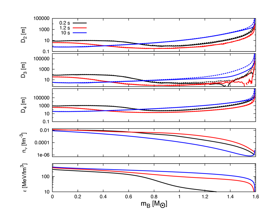
Figure 3: Neutrino diffusion coefficients $D_{n}$ ($n=2,3,4$), as functions of the enclosed baryon mass, computed using the density and thermodynamical profiles of the non-rotating (solid line) and rotating (dashed line) configurations, at $t=0.2$ s, $t=1.2$ s and $t=10$ s (upper and middle panels). Profiles of neutrino number density and energy density (lower panels). We assume $M_{b}=1.6\,M_{\odot}$ and that the angular momentum is the maximum allowed $J_{in}=J_{max}$ (for $J_{in}>J_{max}$, the PNS reaches the mass-shedding limit during its evolution, see Sec. IV.1).

Since we want to model the PNS consistently with the evolutionary models given in Pons et al. (1999), we decided to implement the non-rotating profiles in an alternative way. As in the previous approach, we consider the spherical configuration obtained by the evolution code at time $t$, with central density $p_{c}$ and baryon mass (constant during the evolution) $M_{b}$. To describe the rotating star, we use the GM3 EoS $\epsilon=\epsilon(p,s,Y_{L})$; since we are restricting our analysis to slowly rotating stars, the entropy and lepton fraction profiles $s(a)$ and $Y_{L}(a)$ of the non-rotating star are a good approximation for those of the rotating star. We follow the steps discussed at the end of Section III.1: (i) solve the TOV equations for a star with central pressure $p_{c}+\delta p_{c}$; at each value of $a$, the energy density is $\epsilon(p,s(a),Y_{L}(a))$; (ii) solve Hartle’s perturbation equations, finding the baryon mass of the star rotating to a given rate with this reduced central pressure and find the correction to the baryon mass due to rotation; (iii) iterate the first two steps, finding $\delta p_{c}$ such that the baryon mass of the rotating star is $M_{b}$. We remark that the energy density of the rotating star in step (ii) is related to that of the non-rotating star in step (i) by the Hartle-Thorne prescription described above Eq. (11).

Since we are using an appropriate non-barotropic EoS, the instability discussed above disappears, and the central pressure of the rotating star is, as expected, smaller than that of the non-rotating star with same baryon mass.

We stress again that we are using the numerical solution of the transport equations (5) for a non-rotating PNS, to build quasi-stationary configurations of a rotating PNS. Therefore, we are neglecting the effect of rotation on the time evolution of the PNS. To be consistent, we should have integrated the transport equations appropriate for a rotating star, which are much more complicated. Since these approximations affect the timescale of the stellar evolution, we would like to estimate how faster, or slower, the rotating star looses its thermal and lepton content with respect to the non-rotating one.
Since the evolution timescale is governed by neutrino diffusion processes, at each time step of the non-rotating PNS evolution, we have computed and compared the neutrino diffusion coefficients $D_{n}$ (see Eqns. (6), (7)) for non-rotating and rotating configurations. The latter have been obtained by replacing the profiles ($p(a)$, $\epsilon(a)$, etc.) of a non-rotating PNS with those of a rotating PNS (computed as discussed above in this Section). In the upper and middle panels of Fig. 3 we plot $D_{2},D_{3}$ and $D_{4}$ as functions of the enclosed baryon mass $m_{B}=m_{n}a$, for the non-rotating (solid line) and rotating (dashed line) configurations, at $t=0.2$ s, $t=1.2$ s and $t=10$ s. In the lower panels we plot the neutrino number density and the total energy density at the same times. We assume $M_{b}=1.6\,M_{\odot}$ and that the initial angular momentum, $J_{in}$, is equal to the maximum angular momentum $J_{max}$, above which mass-shedding sets in (see Sec. IV.1 for further details). We see that the diffusion coefficients of the rotating configurations are larger than those of the non-rotating star. For $m_{B}\lesssim 1~{}M_{\odot}$ the relative difference $|D_{n}^{rot}-D_{n}^{non~{}rot}|/|D_{n}^{non~{}rot}|$ is always smaller than $\sim 10-20\%$, and becomes smaller than a few percent after the first few seconds.

In the outer region $m_{B}\gtrsim 1~{}M_{\odot}$ and early times, the relative difference seems larger, in particular for the coefficient $D_{3}$, but this has no effect for two reasons: first, as shown in the two lower panels of Fig. 3, both the neutrino number density and the total energy density are much smaller than in the inner core; therefore, even though the diffusion coefficients of the rotating star are larger than those of the non-rotating one, few neutrinos are trapped in this region and transport effects do not contribute significantly to the overall evolution; second, the differences become large in the semi-transparent region, when the mean free path becomes comparable to (or larger than) the distance to the star surface. In this region the diffusion approximation breaks down and in practice the diffusion coefficients are always numerically limited (a flux-limiter approach).

From the above discussion we can conclude that the rotating star looses energy and lepton number through neutrino emission faster than the non-rotating one. This effect is larger at the beginning of the evolution, i.e. for $t\lesssim 2$ s, and is of the order of $\sim 10-20\%$, but becomes negligible at later times. Consequently our rotating star cools down and contracts over a timescale which, initially, is $\sim 10-20\%$ shorter than that of the corresponding non-rotating configuration.

III.3 Evolution of the angular momentum and of the rotation rate

Once the equations describing the rotating configuration are solved for each value of the evolution time $t$ and for an assigned value of the rotation rate $\Omega$, the solution of these equations allows one to compute the multipole moments of the rotating star, including the angular momentum $J$. Conversely we can choose, at each value of $t$, the value of the angular momentum, and determine, using a shooting method, the corresponding value of the rotation rate.

If we want to describe the early evolution of a rotating PNS, we need a physical prescription for the time dependence of $J$. For instance, we may assume that the angular momentum is constant, as in Villain et al. (2004) (see also Goussard et al. (1997, 1998)). However, in the first minute of a PNS life, neutrino emission carries away $\sim 10\%$ of the star gravitational mass Lattimer and Prakash (2001), and also a significant fraction of the total angular momentum Janka (2004). To our knowledge, the most sensible estimate of the neutrino angular momentum loss in PNSs has been done by Epstein in Epstein (1978)

$$\frac{dJ}{dt}=-\frac{2}{5}qL_{\nu}R^{2}\Omega$$ (12)

where $R$ is the radius of the star, $L_{\nu}=-dM/dt$ is the neutrino energy flux, and $q$ is an efficiency parameter, which depends on the features of the neutrino transport and emission. If neutrinos escape without scattering, $q=1$; if, instead, they have a very short mean free path, they are diffused up to the surface, and then are emitted with $q=5/3$. As discussed in Epstein (1978) (see also Kazanas (1977); Mikaelian (1977); Henriksen and Chau (1978)), $q=5/3$ should be considered as an upper limit of the angular momentum loss by neutrino emission. A more recent, alternative study Dvornikov and Dib (2010) indicates an angular momentum emission smaller than this limit. In the following, we shall consider Epstein’s formula with $q=5/3$, and this has to be meant as an upper limit. We also mention that a simplified expression based on Epstein’s formula for the angular momentum loss in PNSs has been derived in Janka (2004) and used in Martinon et al. (2014).

III.4 Mass-shedding frequency

As mentioned in Sec. III.1, the perturbative approach which we use to model a rotating star is accurate up to $\nu\lesssim 0.8\nu_{ms}$, where $\nu_{ms}$ is the mass-shedding frequency. The only quantity which is poorly estimated is, of course, the mass-shedding frequency itself. Therefore, $\nu_{ms}$ will be determined using a numerical fit derived in Doneva et al. (2013) from fully relativistic, non-linear integrations of Einstein’s equations:

$$\nu_{ms}(Hz)=a\sqrt{\frac{M/M_{\odot}}{R/1{\rm km}}}+b$$ (13)

where $a=45862$ Hz and $b=-189$ Hz. We remark that the coefficients $a,b$ of this fit do not depend on the EoS.

III.5 Gravitational wave emission

If the evolving PNS is born with some degree of asymmetry, it emits gravitational waves. Assuming that the star rotates about a principal axis of the moment of inertia tensor, i.e., that there is no precession, gravitational waves are emitted at twice the orbital frequency $\nu$, with amplitude Zimmermann and Szedenits (1979); Thorne (1987); Bonazzola and Gourgoulhon (1996); Jones (2002)

$$h_{0}\simeq\frac{4G(2\pi\nu)^{2}I_{3}\epsilon}{c^{4}r}\,.$$ (14)

The deviation from axisymmetry is described by the ellipticity $\epsilon$, defined as

$$\epsilon=\frac{I_{1}-I_{2}}{I_{3}}$$ (15)

where $I_{1}$, $I_{2}$ and $I_{3}$ are the principal moments of inertia of the PNS and $I_{3}$ is assumed to be aligned with the rotation axis. For old neutron stars, the loss of energy through gravitational waves is compensated by a decrease of rotational energy, which contributes to the spin-down of the star (the main contribution to the spin-down being that of the magnetic field).

In the case of a newly born PNS the situation is different. As the star contracts, due to the processes related to neutrino production and diffusion, its rotation rate increases. If the PNS has a finite ellipticity, it emits gravitational waves, whose amplitude and frequency also increase as the star spins up. The timescale of this process is of the order of tens of seconds. In our model, for simplicity we shall assume that the PNS ellipticity remains constant over this short time interval.

Unfortunately, the ellipticity of a PNS is unknown. In cold, old NSs it is expected to be, at most, as large as $\sim 10^{-5}-10^{-4}$ Haskell et al. (2006); Ciolfi et al. (2010) (larger values are allowed for EoS including exotic matter phases Horowitz and Kadau (2009); Johnson-McDaniel and Owen (2013)). For newly born PNSs, it may be larger, but we have no hint on its actual value. To our knowledge, current numerical simulations of core-collapse do not provide estimates of the PNS ellipticity. We remark that although there is observational evidence of large asymmetries in supernova explosions Wang et al. (2003); Leonard et al. (2006), there is no evidence that they can be inherited by the PNS. In the following, we shall assume $\epsilon=10^{-4}$, but this should be considered as a fiducial value: the gravitational wave amplitude (which is linear in $\epsilon$) can be easily rescaled for different values of the PNS ellipticity.

IV Results

IV.1 Spin evolution of the proto-neutron star

In Figure 4 we show how the angular momentum changes according to Epstein’s formula (12) as the PNS evolves. We assume $q=5/3$ and baryonic mass $M_{b}=1.6\,M_{\odot}$. We consider different values of the angular momentum $J_{in}$ at the beginning of the quasi-stationary phase ($t=0.2$ s after the bounce): $J_{in}=2.02\times 10^{48}\,\mathrm{erg\,s}$, $J_{in}=3.71\times 10^{48}\,\mathrm{erg\,s}$ and $J_{in}=8.08\times 10^{48}\,\mathrm{erg\,s}$. We find that, in the first ten seconds after bounce, $13\%$ of the initial angular momentum is carried away by neutrinos if $J_{in}=2.02\times 10^{48}\,\mathrm{erg\,s}$ or $J_{in}=3.71\times 10^{48}\,\mathrm{erg\,s}$; $20\%$ of the initial angular momentum is carried away if $J_{in}=8.075\times 10^{48}\,\mathrm{erg\,s}$. As mentioned above, $q=5/3$ should be considered as an upper bound; for smaller values of $q$, the rate of angular momentum loss would be smaller.

Figure 4: Angular momentum evolution due to neutrino losses, for a PNS with baryonic mass $M_{b}=1.6\,M_{\odot}$ and initial angular momentum $J_{in}=(2.02,\,3.71,\,8.08)\times 10^{48}$erg s.

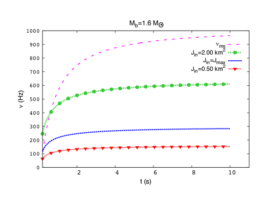
Figure 5: Evolution of the PNS rotation rate, corresponding to the angular momentum profiles shown in Figure 4.

The corresponding evolution of the PNS rotation frequency is shown in Figure 5. In the same Figure we also show the mass-shedding frequency $\nu_{ms}$, computed using the fit (13). We see that if $J_{in}=8.08\times 10^{48}\,\mathrm{erg\,s}$, the curves of $\nu(t)$ and of $\nu_{ms}(t)$ cross during the quasi-stationary evolution; before the crossing, the PNS spin is larger than the mass-shedding limit. This means that a PNS with such initial angular momentum would lose mass. If we require the initial rotation rate to be smaller than the mass-shedding limit, we must impose $J_{in}\leq J_{max}\equiv 3.72\times 10^{48}\,\mathrm{erg\,s}$. We remark that the value of $J_{max}$ is not affected by the efficiency of angular momentum loss $q$: if $q<5/3$, $J_{max}$ has the same value, but the rotation rate grows more rapidly than in Figure 5.

It is interesting to note that, since $\nu_{ms}$ has a steeper increase than $\nu(t)$, even when the bound $\nu\leq\nu_{ms}$ is saturated at the beginning of the quasi-stationary phase the frequency becomes much smaller than the mass shedding frequency at later times. This is an a-posteriori confirmation that the slow rotation approximation is appropriate to study newly born PNSs. For $t>10$ s, the PNS radius does not change significantly, and the star starts to spin down due to electromagnetic and gravitational emission. However this spindown timescale is much longer than the timescale of the quasi-stationary evolution we are considering; therefore it is unlikely that after this early phase the PNS rotation rate is larger than $\sim 300$ Hz (i.e., that its period is smaller than $\sim 3$ ms), unless some spin-up mechanism (such as e.g. accretion) sets in. A less efficient angular momentum loss ($q<5/3$) would moderately increase this final value, but the general picture would remain the same.

It is worth noting that models of pre-supernova stellar evolution Heger et al. (2005) predict a similar range of the PNS rotation rate and angular momentum. Among the models considered in Heger et al. (2005), the only one with $J>J_{max}$ (and rotation period smaller than $3$ ms) is expected to collapse to a black hole. Other works Thompson et al. (2005); Ott et al. (2006) have shown that if the progenitor has a rotation rate sufficiently large, the PNS resulting from the core-collapse can have periods of few ms; our results suggest that this scenario is unlikely, unless there is a significant mass loss in the early Kelvin-Helmoltz phase.

IV.2 Gravitational wave emission

If the PNS has a finite ellipticity $\epsilon$ (which we assume, for simplicity, to remain constant during the first $\sim 10$ s of the PNS life), it emits gravitational waves with frequency $f(t)=2\nu(t)$ and amplitude given by Eq. (14),

$$h_{0}\simeq\frac{4G(2\pi\nu(t))^{2}I_{3}(t)\epsilon}{c^{4}r}\,.$$ (16)

As the spin rate $\nu(t)$ increases, both the frequency and the amplitude of the gravitational wave increase; therefore, the signal is a sort of “chirp”; this is different from the chirp emitted by neutron star binaries before coalescence, because the amplitude increases at a much milder rate. In Figure 6 we show the strain amplitude $\tilde{h}(f)\sqrt{f}=\sqrt{f}\sqrt{(\tilde{h}_{+}(f)^{2}+\tilde{h}_{\times}(f)^{2})/2}$, where $\tilde{h}_{+,\times}(f)$ are the Fourier transform of the two polarization of the gravitational wave signal

$$h_{+} = h_{0}\frac{1+\cos^{2}i}{2}\cos(2\pi f(t)t)$$ (17)

$$h_{\times} = h_{0}\cos i\sin(2\pi f(t)t),$$ (18)

and $i$ is the angle between the rotation axis and the line of sight. In Figure 6 the signal strain amplitude, computed assuming optimal orientation, $J_{in}=J_{max}$, $\epsilon=10^{-4}$ and a distance of $r=10$ kpc, is compared with the sensitivity curves of Advanced Virgo, Advanced LIGO, and of the third generation detector ET. We see that the signal is marginally above noise for the advanced detectors, but it is definitely above the noise curve for ET. This signal would be seen by Advanced Virgo with a signal-to-noise ratio $SNR=1.4$, and by Advanced LIGO with $SNR=2.2$, too low to extract it from the detector noise; however, since the signal-to-noise ratio scales linearly with the ellipticity, a star born with $\epsilon=10^{-3}$ would be detected with $SNR=14$ and $SNR=22$ by Advanced Virgo and LIGO, respectively. The third generation detectors like ET would detect the signal coming from a galactic PNS born with $\epsilon=10^{-4}$ with a very large signal-to-noise ratio, i.e. $SNR=22$. If the source is in the Virgo cluster ($d=15~{}Mpc$), the ellipticity of the PNS should be as large as $5\cdot 10^{-2}$ to be seen by ET with $SNR=8$.

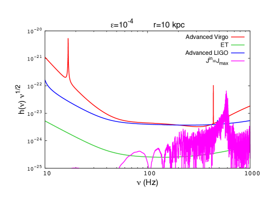
Figure 6: The strain amplitude $\tilde{h}(f)\sqrt{f}$ of the gravitational wave signal emitted by a PNS with $\epsilon=10^{-4}$, $J_{in}=J_{max}$, at a distance $r=10$ kpc, is compared with the noise curves of Advanced Virgo, Advanced LIGO and ET.

V Concluding remarks

In this paper we have studied the angular momentum loss, the time dependence of the rotation rate and the gravitational wave emission of a newly born PNS, during the first tens of seconds after bounce. The early evolution of the rotating PNS has been modeled using the entropy and lepton fraction profiles consistently computed solving the general relativistic transport equations for a non-rotating star; angular momentum loss due to neutrino emission has been modeled using Epstein’s formula Epstein (1978).

During this early evolution, the star spins up due to contraction. By requiring that the initial rotation rate does not exceed the mass-shedding limit, we have estimated the maximum rotation rate at the end of the spin-up phase. For a PNS of $M_{b}=1.6\,M_{\odot}$ we find that one minute after bounce the star would rotate at $\nu\lesssim 300$ Hz, corresponding to a rotation period $\tau_{min}\gtrsim 3.3\times 10^{-3}\,\mathrm{s}$.

If the PNS is born with a finite ellipticity $\epsilon$, while spinning up it emits gravitational waves at twice the rotation frequency. This signal increases both in frequency and amplitude. We find that for a galactic supernova, if $\epsilon=10^{-3}$ this signal could be detected by Advanced LIGO/Virgo with a signal-to-noise ratio $\gtrsim 14$. To detect farther sources, third generation detectors like ET would be needed.

We remark that the actual value of PNS ellipticities is unknown, and depends on the details of the supenova core collapse. Accurate numerical simulations of supernova explosion addressing this issue are certainly needed to provide a quantitative estimate of the range of $\epsilon$.

We also remark that in our approach the effects of the PNS rotation are consistently included in the structure equations, but they are neglected when solving the neutrino transport equations. We estimate that due to this approximation, we overestimate the evolution timescale at early times of, at most, $\sim 10-20\%$. Moreover, since we are not interested in the details of the neutrino dynamics and we need a fast code to evolve the star for tens of seconds, we perform energy averages to determine the neutrino diffusion coefficients, and we apply a flux-limiter; these approximations should not significantly affect the thermodynamical evolution of the PNS and its gravitational wave emission.

This work is a first step in the study of the early evolution of PNSs. A paper with a detailed description of our numerical code, and its extension to more recent EoSs, is in preparation Camelio et al. (2016). Further developments shall include differential rotation, convection and generalization of the neutrino transport equations to rotating PNSs.

Appendix A Hartle-Thorne equations

Here, we briefly describe the equations of the perturbative Hartle-Thorne approach discussed in Sec. III.1. For further details we refer the reader to Hartle (1967); Hartle and Thorne (1968); Hartle (1973) and to the Appendix of Benhar et al. (2005).

The spacetime metric (up to order $O(\Omega^{3})$) is given by Eq. (III.1); it depends on the background functions $\phi(r)$, $\lambda(r)=-\log(1-2m(r)/r)$, and on the perturbations functions $h_{l}(r)$, $m_{l}(r)$ ($l=0,2$), $k_{2}(r)$, $\omega(r)$, $w_{l}(r)$ ($l=1,3$). The energy and pressure (Eulerian) perturbations are

$$\delta P = (\epsilon(r)+P(r))(\delta p_{0}(r)+\delta p_{2}(r)P_{2}(\mu))$$

$$\delta\epsilon = \frac{d\epsilon/dr}{dP/dr}\delta P\,,$$ (19)

and depend on the perturbation functions $p_{l}(r)$ ($l=0,2$).

The background spacetime is described by the TOV equations:

$$\frac{dm}{dr} = 4\pi r^{2}\epsilon$$

$$\frac{d\phi}{dr} = 2\frac{m+4\pi r^{3}P}{r(r-2m)}$$

$$\frac{dP}{dr} = -\frac{\epsilon+P}{2}\frac{d\phi}{dr}\,.$$ (20)

The mass of the non-rotating configuration is obtained by matching at the stellar surface $r=R$ the interior solution with the exterior (Schwarzschild) solution, i.e., $M=m(R)$. Moreover, the baryonic mass $M_{b}$ of the non-rotating configuration is obtained integrating the equation $dm_{b}/dr=4\pi r^{2}e^{\lambda/2}\rho$, and computing $M_{b}=m_{b}(r)$.

The spacetime perturbation to first order in $\Omega$ is described by the function $\omega(r)$, which is responsible for the dragging of inertial frames; it satisfies the equations

$$\frac{d\chi}{dr} = \frac{u}{r^{4}}-\frac{4\pi r^{2}(\epsilon+P)\chi}{r-2M}$$ (21)

$$\frac{du}{dr} = \frac{16\pi r^{5}(\epsilon+P)\chi}{r-2M}\,,$$ (22)

where $\varpi=\Omega-\omega$, $j(r)=e^{-\phi/2}(1-2M/r)^{1/2}$, $\chi=j\varpi$ and $u=r^{4}jd\varpi/dr$. The angular momentum $J$ is obtained by matching the interior with the exterior solution $\chi(r)=\Omega-2J/r^{3}$, $u(r)=6J$ at $r=R$. The moment of inertia, at zero-th order in the rotation rate, is $I=J/\Omega$.

The perturbations to second order in $\Omega$ are described by the metric functions $h_{l}(r)$, $m_{l}(r)$ ($l=0,2$), $k_{2}(r)$, and by the fluid pressure perturbations $\delta p_{l}$. The $l=0$ perturbations satisfy the equations

$$\frac{d}{dr}\left(\delta p_{0}+h_{0}-\frac{\chi^{2}r^{3}}{3(r-2M)}\right) = 0$$

$$\delta p_{2}+h_{2}-\frac{\chi^{2}r^{3}}{3(r-2M)} = 0$$

and

$$\frac{dm_{0}}{dr} = 4\pi r^{2}\frac{d\epsilon}{dP}[\delta p_{0}(\epsilon+P)]+\frac{u^{2}}{12r^{4}}+\frac{8\pi r^{5}(\epsilon+P)\chi^{2}}{3(r-2M)}$$

$$\frac{d\delta p_{0}}{dr} = \frac{u^{2}}{12r^{4}(r-2M)}-\frac{m_{0}(1+8\pi r^{2}P)}{(r-2M)^{2}}$$ (24)

$$-\frac{4\pi(\epsilon+P)r^{2}\delta p_{0}}{r-2M}+\frac{2r^{2}\chi}{3(r-2M)}\left[\frac{u}{r^{3}}\right.$$

$$\left.+\frac{(r-3M-4\pi r^{3}P)\chi}{r-2M}\right]\,.$$

Matching the interior and the exterior solutions at $r=R$, it is possible to compute the correction to the mass due to stellar rotation, $\delta M=m_{0}(R)+J^{2}/R^{3}$, and the monopolar stellar deformation. The baryonic mass correction $\delta M_{b}=\delta m_{b}(R)$ is given by solving the equation

$$\frac{d\delta m_{b}}{dr} = 4\pi r^{2}e^{\lambda/2}\left[\left(1+\frac{m_{0}}{r-2m}+\frac{1}{3}r^{2}\varpi^{2}e^{-\phi}\right)\epsilon\right.$$ (25)

$$\left.+\frac{d\epsilon/dr}{dP/dr}(\epsilon+P)\delta p_{0}\right]\,.$$

The $l=2$ perturbations satisfy the equations

$$\frac{dv_{2}}{dr} = -\frac{d\phi}{dr}h_{2}+(\frac{1}{r}+\frac{1}{2}\frac{d\phi}{dr})\left[\frac{8\pi r^{5}(\epsilon+P)\chi^{2}}{3(r-2M)}+\frac{u^{2}}{6r^{4}}\right]$$

$$\frac{dh_{2}}{dr} = \left[-\frac{d\phi}{dr}+\frac{r}{r-2M}(\frac{d\phi}{dr})^{-1}(8\pi(\epsilon+P)-\frac{4M}{r^{3}})\right]h_{2}$$ (26)

$$- \frac{4v_{2}}{r(r-2M)}(\frac{d\phi}{dr})^{-1}+\frac{u^{2}}{6r^{5}}\left[\frac{1}{2}\frac{d\phi}{dr}r-\frac{1}{r-2M}(\frac{d\phi}{dr})^{-1}\right]$$

$$+ \frac{8\pi r^{5}(\epsilon+P)\chi^{2}}{3(r-2M)}\left[\frac{1}{2}\frac{d\phi}{dr}r+\frac{1}{r-2M}(\frac{d\phi}{dr})^{-1}\right]\,,$$

where $v_{2}=k_{2}+h_{2}$. Matching the interior and exterior solutions, it is possible to determine the quadrupole moment of the PNS and its quadrupolar deformation.

The equations for the peturbations at $O(\Omega^{3})$, $w_{l}(r)$ ($l=1,3$), have a similar structure but they are longer and are not reported here; we refer the reader to Hartle (1973); Benhar et al. (2005). They yield the octupole moment, the third-order corrections to the angular momentum and the second-order corrections to the moment of inertia.

References

- Burrows and Lattimer (1986) A. Burrows and J. M. Lattimer, Astrophys. J. 307, 178 (1986).
- Keil and Janka (1995) W. Keil and H. T. Janka, Astron. Astrophys. 296, 145 (1995).
- Pons et al. (1999) J. A. Pons, S. Reddy, M. Prakash, J. M. Lattimer, and J. A. Miralles, Astrophys. J. 513, 780 (1999), arXiv:astro-ph/9807040 [astro-ph] .
- Ferrari et al. (2003) V. Ferrari, G. Miniutti, and J. A. Pons, Mon. Not. Roy. Astron. Soc. 342, 629 (2003), arXiv:astro-ph/0210581 [astro-ph] .
- Ott (2009) C. D. Ott, Class. Quant. Grav. 26, 063001 (2009), arXiv:0809.0695 [astro-ph] .
- Burgio et al. (2011) G. F. Burgio, V. Ferrari, L. Gualtieri, and H. J. Schulze, Phys. Rev. D84, 044017 (2011), arXiv:1106.2736 [astro-ph.SR] .
- Fuller et al. (2015) J. Fuller, H. Klion, E. Abdikamalov, and C. D. Ott, Mon. Not. Roy. Astron. Soc. 450, 414 (2015), arXiv:1501.06951 [astro-ph.HE] .
- Heger et al. (2005) A. Heger, S. E. Woosley, and H. C. Spruit, Astrophys. J. 626, 350 (2005), arXiv:astro-ph/0409422 [astro-ph] .
- Thompson et al. (2005) T. A. Thompson, E. Quataert, and A. Burrows, Astrophys. J. 620, 861 (2005), arXiv:astro-ph/0403224 [astro-ph] .
- Ott et al. (2006) C. D. Ott, A. Burrows, T. A. Thompson, E. Livne, and R. Walder, Astrophys. J. Suppl. 164, 130 (2006), arXiv:astro-ph/0508462 [astro-ph] .
- Hanke et al. (2013) F. Hanke, B. Mueller, A. Wongwathanarat, A. Marek, and H.-T. Janka, Astrophys. J. 770, 66 (2013), arXiv:1303.6269 [astro-ph.SR] .
- Couch and Ott (2015) S. M. Couch and C. D. Ott, Astrophys. J. 799, 5 (2015), arXiv:1408.1399 [astro-ph.HE] .
- Nakamura et al. (2014) K. Nakamura, T. Kuroda, T. Takiwaki, and K. Kotake, Astrophys. J. 793, 45 (2014), arXiv:1403.7290 [astro-ph.HE] .
- Miller and Miller (2014) M. C. Miller and J. M. Miller, Phys. Rept. 548, 1 (2014), arXiv:1408.4145 [astro-ph.HE] .
- Pons et al. (2001a) J. A. Pons, J. A. Miralles, M. Prakash, and J. M. Lattimer, Astrophys. J. 553, 382 (2001a), arXiv:astro-ph/0008389 [astro-ph] .
- Pons et al. (2001b) J. A. Pons, A. W. Steiner, M. Prakash, and J. M. Lattimer, Phys. Rev. Lett. 86, 5223 (2001b), arXiv:astro-ph/0102015 [astro-ph] .
- Roberts (2012) L. F. Roberts, Astrophys. J. 755, 126 (2012), arXiv:1205.3228 [astro-ph.HE] .
- Ferrari et al. (2004) V. Ferrari, L. Gualtieri, J. A. Pons, and A. Stavridis, Mon. Not. Roy. Astron. Soc. 350, 763 (2004), arXiv:astro-ph/0310896 [astro-ph] .
- Villain et al. (2004) L. Villain, J. A. Pons, P. Cerda-Duran, and E. Gourgoulhon, Astron. Astrophys. 418, 283 (2004), arXiv:astro-ph/0310875 [astro-ph] .
- Gourgoulhon et al. (1999) E. Gourgoulhon, P. Haensel, R. Livine, E. Paluch, S. Bonazzola, and J. A. Marck, Astron. Astrophys. 349, 851 (1999), arXiv:astro-ph/9907225 [astro-ph] .
- Martinon et al. (2014) G. Martinon, A. Maselli, L. Gualtieri, and V. Ferrari, Phys. Rev. D90, 064026 (2014), arXiv:1406.7661 [gr-qc] .
- Epstein (1978) R. Epstein, Astrophys. J. 219, L39 (1978).
- Camelio et al. (2016) G. Camelio, L. Gualtieri, G. Lovato, O. Benhar, J. A. Pons, M. Fortin, and V. Ferrari, (2016), in preparation.
- Glendenning and Moszkowski (1991) N. K. Glendenning and S. A. Moszkowski, Phys. Rev. Lett. 67, 2414 (1991).
- Levermore and Pomraning (1981) C. Levermore and G. Pomraning, The Astrophysical Journal 248, 321 (1981).
- Wilson and Mayle (1989) J. R. Wilson and R. W. Mayle, in NATO Advanced Science Institutes (ASI) Series B, NATO Advanced Science Institutes (ASI) Series B, Vol. 216, edited by W. Greiner and H. Stöcker (1989) p. 731.
- Hartle (1967) J. B. Hartle, Astrophys. J. 150, 1005 (1967).
- Hartle and Thorne (1968) J. B. Hartle and K. S. Thorne, Astrophys. J. 153, 807 (1968).
- Benhar et al. (2005) O. Benhar, V. Ferrari, L. Gualtieri, and S. Marassi, Phys. Rev. D72, 044028 (2005), arXiv:gr-qc/0504068 [gr-qc] .
- Janka and Mönchmeyer (1989) H.-T. Janka and R. Mönchmeyer, Astronomy and Astrophysics 226, 69 (1989).
- Mösta et al. (2015) P. Mösta, C. D. Ott, D. Radice, L. F. Roberts, E. Schnetter, and R. Haas, Nature 528, 376 (2015), arXiv:1512.00838 [astro-ph.HE] .
- O’Connor and Ott (2010) E. O’Connor and C. D. Ott, Classical and Quantum Gravity 27, 114103 (2010), arXiv:0912.2393 [astro-ph.HE] .
- Goussard et al. (1997) J.-O. Goussard, P. Haensel, and J. L. Zdunik, Astron. Astrophys. 321, 822 (1997), arXiv:astro-ph/9610265 [astro-ph] .
- Goussard et al. (1998) J. O. Goussard, P. Haensel, and J. L. Zdunik, Astron. Astrophys. 330, 1005 (1998), arXiv:astro-ph/9711347 [astro-ph] .
- Lattimer and Prakash (2001) J. M. Lattimer and M. Prakash, Astrophys. J. 550, 426 (2001), arXiv:astro-ph/0002232 [astro-ph] .
- Janka (2004) H.-T. Janka, IAU Symposium 218: Young Neutron Stars and Their Environment Sydney, Australia, July 14-17, 2003, (2004), [IAU Symp.218,3(2004)], arXiv:astro-ph/0402200 [astro-ph] .
- Kazanas (1977) D. Kazanas, Nature (London) 267, 501 (1977).
- Mikaelian (1977) K. O. Mikaelian, Astrophys. J. 214, L23 (1977).
- Henriksen and Chau (1978) R. N. Henriksen and W. Y. Chau, Astrophys. J. 225, 712 (1978).
- Dvornikov and Dib (2010) M. Dvornikov and C. Dib, Phys. Rev. D82, 043006 (2010), arXiv:0907.1445 [astro-ph.HE] .
- Doneva et al. (2013) D. D. Doneva, E. Gaertig, K. D. Kokkotas, and C. Krüger, Phys. Rev. D88, 044052 (2013), arXiv:1305.7197 [astro-ph.SR] .
- Jones and Andersson (2001) D. I. Jones and N. Andersson, Mon. Not. Roy. Astron. Soc. 324, 811 (2001), arXiv:astro-ph/0011063 [astro-ph] .
- Suwa (2014) Y. Suwa, Publ. Astron. Soc. Jap. 66, L1 (2014), arXiv:1311.7249 [astro-ph.HE] .
- Zimmermann and Szedenits (1979) M. Zimmermann and E. Szedenits, Phys. Rev. D20, 351 (1979).
- Thorne (1987) K. S. Thorne, “Gravitational radiation.” in Three Hundred Years of Gravitation, edited by S. W. Hawking and W. Israel (1987) pp. 330–458.
- Bonazzola and Gourgoulhon (1996) S. Bonazzola and E. Gourgoulhon, Astron. Astrophys. 312, 675 (1996), arXiv:astro-ph/9602107 [astro-ph] .
- Jones (2002) D. I. Jones, Gravitational waves. Proceedings, 4th Edoardo Amaldi Conference, Amaldi 4, Perth, Australia, July 8-13, 2001, Class. Quant. Grav. 19, 1255 (2002), arXiv:gr-qc/0111007 [gr-qc] .
- Haskell et al. (2006) B. Haskell, D. I. Jones, and N. Andersson, Mon. Not. Roy. Astron. Soc. 373, 1423 (2006), arXiv:astro-ph/0609438 [astro-ph] .
- Ciolfi et al. (2010) R. Ciolfi, V. Ferrari, and L. Gualtieri, Mon. Not. Roy. Astron. Soc. 406, 2540 (2010), arXiv:1003.2148 [astro-ph.SR] .
- Horowitz and Kadau (2009) C. J. Horowitz and K. Kadau, Phys. Rev. Lett. 102, 191102 (2009), arXiv:0904.1986 [astro-ph.SR] .
- Johnson-McDaniel and Owen (2013) N. K. Johnson-McDaniel and B. J. Owen, Phys. Rev. D88, 044004 (2013), arXiv:1208.5227 [astro-ph.SR] .
- Wang et al. (2003) L. Wang, D. Baade, P. Hoeflich, J. C. Wheeler, C. Fransson, and P. Lundqvist, Astrophys. J. 592, 457 (2003), arXiv:astro-ph/0206386 [astro-ph] .
- Leonard et al. (2006) D. C. Leonard et al., Nature 440, 505 (2006), arXiv:astro-ph/0603297 [astro-ph] .
- Hartle (1973) J. B. Hartle, Astrophysics and Space Science 24, 385 (1973).